Broadband Coherent Perfect Absorber with $\mathcal{P}\mathcal{T}$-Symmetric 2D-Materials

Abstract

We suggest graphene and a two-dimensional (2D) Weyl semimetal (WSM) as 2D materials for the realization of a broadband coherent perfect absorber (CPA) respecting overall $\mathcal{PT}$-symmetry. We also demonstrate the conditions for mutually equal amplitudes and phases of the left and right incoming waves to realize a CPA. 2D materials in our system play the role to enhance the absorption rate of a CPA once the appropriate parameters are inserted in the system. We show that a 2D WSM is more effective than graphene in obtaining the optimal conditions. We display the behavior of each parameter governing the optical system and show that optimal conditions of these parameters give rise to enhancement and possible experimental realization of a broadband CPA-laser.

Keywords: Coherent Perfect Absorption, Spectral Singularity, PT Symmetry, Graphene, Weyl Semimetal, 2D Materials

1 Introduction

Time-reversed consideration of regular lasers come into existence by purely ingoing fields, which is known as coherent perfect absorption (CPA), or antilaser [1, 2, 3, 4, 5, 6, 7, 8]. This intriguing phenomenon has made a rather drastic influence in nanostructured optical materials and especially in plasmonics [9], and recently has attracted a broad interest. They underlie many applications, including molecular sensing, photocurrent generation and photodetection [8]. In a CPA, complete absorption at a single frequency can be achieved by illuminating two counter propagating fields [10, 11], see [8] for a recent review of CPAs. Time reversal symmetry reveals the condition that a CPA supports the self-dual spectral singularities [12, 13, 14, 15]. Since the time reversal symmetry incorporates CPA action to lasing threshold condition, it comes out to be a natural consequence of $\mathcal{PT}$-symmetric potentials that support both CPA and laser actions simultaneously [3]. This makes $\mathcal{PT}$-symmetric CPA-lasers one of the primary examples in the study of optics [12], and also rather intriguing because of its function as a laser emitting coherent waves unless it is subject to incident coherent waves with appropriate amplitude and phase in which case it acts as an absorber [11]. In this work, we investigate the prospect of realizing a broadband CPA-laser in a linear homogeneous $\mathcal{PT}$-symmetric optical system covered by two-dimensional (2D) materials. We set out the prescribed 2D materials as the absorbing medium, and employ their prominent features in smooth experimental achievement of a CPA which consists of equal amplitudes and phases of incoming waves.

$\mathcal{PT}$-symmetry in optical systems is achieved by means of complex refractive indices, such that their optical modulations in complex dielectric permittivity plane results in both optical absorption and amplification. $\mathcal{PT}$-symmetry is rather practical in optics since it helps related parameters of the optical system be adjusted properly. Thus, $\mathcal{PT}$-symmetric optical systems [16, 17, 18] are currently studied actively due to their applications in a series of intriguing optical phenomena and devices, such as dynamic power oscillations of light propagation, lasers [13, 14, 15, 19, 20], CPA lasers [11, 21, 22, 23, 24, 25, 26], and unidirectional invisibility [16, 17, 18, 27, 28, 29, 30]. CPA phenomenon has become one of leading applications of $\mathcal{PT}$-symmetric optical potentials since its emergence [1].

Discovery of graphene led to over a decade of its intense study. It has triggered development of a vast area of research on a variety of 2D materials, whose properties substantially differ from those of their bulk counterparts [31]. Graphene is arguably the most famous 2D material of the last decade, and fascination with its properties has spread beyond the scientific community. Emergence of graphene has led to arise a voluminous literature and numerous applications has been carried out in various fields [32, 33, 34, 35, 36, 37, 38, 39]. As the family of 2D materials expanded to include new members such as 2D Weyl semimetals (WSM), 2D semiconductors, boron nitride and more recently, transition metal dichalcogenides and Xenes, atomically thin forms of these materials offer endless possibilities for fundamental research, as well as demonstration of improved or even entirely novel technologies [40, 41, 42]. In view of these exciting properties of 2D materials together with the idea that they may interact with electromagnetic waves in anomalous and exotic ways, providing new phenomena and applications, the new distinctive studies of laser and CPA phenomena with 2D materials have arisen. Especially recent works on this field fashion up essential motivation of our work [11, 43, 44, 45, 46, 47], which will use the whole competency of transfer matrix method in a scattering formalism [48]. In this study, we offer one of the potential applications of 2D materials in the field of CPA laser actions together with fascinating $\mathcal{PT}$-symmetry attribute in optical systems. Our system is depicted in Fig. 1.

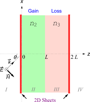
Figure 1: (Color online) TE mode configuration for the parallel pair of optically active system covered by the 2D material sheets obeying the $\mathcal{PT}$-symmetry.

We employ a one-dimensional $\mathcal{PT}$-symmetric optically active system which is covered by a 2D material, which respects the entire $\mathcal{PT}$-symmetry, see Fig. 1. Since CPA conditions coincide with the lasing threshold conditions, both of which could be expressed by means of spectral singularities, the former is typically expressed by self-dual spectral singularities which is complex conjugate of spectral singularities. We look for practical ways to improve the efficiency of CPA through the supplemented coating materials. Although our formalism is satisfied by all 2D materials, for the likeliest demonstration we use graphene and 2D WSM, and compare their impacts saliently.

We reveal complete solutions, schematically demonstrate their behaviors and show the effects of various parameter choices yielding CPA conditions. We demonstrate that optimal control of parameters of the slab (gain coefficient, incidence angle and slab thickness). Relevant parameters of 2D material give rise to a desired outcome of achieving enhancement of broadband absorption, and computing correct amplitude and phase contrasts in a CPA-laser. We present exact conditions causing the achievement of CPA with equal amplitude and phase values of ingoing waves. We display the roles of 2D material in the gain decrement, broadband absorption and reciprocities of amplitudes and phases in the production a CPA action. Results of this study show that 2D WSM is more appropriate compared to graphene since it leads to build up a CPA with minimum gain values at a critical $b$ value, below which no effect is observed. Also, 2D WSM helps to improve the broadband accessibility of CPA based on the corresponding parameter adjustments. We provide certain parameters belonging to our system setup if one desires experimental realization of a broadband CPA with equal wave amplitudes and phases.

2 TE Mode Solution, Transfer Matrix and CPA Condition

TE mode Helmholtz equation describing our optical setup in Fig. 1 reads as

$$\left[\nabla^{2}+k^{2}\mathfrak{z}_{j}(z)\right]\vec{E}^{j}(\vec{r})=0, \vec{H}^{j}(\vec{r})=-\frac{i}{kZ_{0}}\vec{\nabla}\times\vec{E}^{j}(\vec{r}).$$ (1)

Its solution yields TE waves in the form

$$\vec{E}^{j}(\vec{r})=\mathcal{E}^{j}(z)e^{ik_{x}x}\hat{e}_{y}.$$ (2)

In this formulation, $\vec{r}:=(x,y,z)$ represents the coordinates, $k:=\omega/c$ is the wavenumber, $c:=1/\sqrt{\mu_{0}\varepsilon_{0}}$ is the speed of light in vacuum, $Z_{0}:=\sqrt{\mu_{0}/\varepsilon_{0}}$ is the impedance of the vacuum, $\hat{e}_{y}$ is the unit vector in $y$-direction, $k_{x}$ and $k_{z}$ are the components of wavevector $\vec{k}$ in $x-z$ plane. Complex quantity $\mathfrak{z}_{j}(z)$ is denoted by

$$\mathfrak{z}_{j}(z):={\mathfrak{n}}_{j}^{2}~{}~{}~{}~{}~{}{\rm for~{}}z\in z_{j}.$$ (3)

The index $j$ represents the regions in Fig. 1 and $j=1,2,3,~{}\textrm{and}~{}4$. Note that refractive indices in regions I and IV are ${\mathfrak{n}}_{1}={\mathfrak{n}}_{4}=1$, whereas ${\mathfrak{n}}_{2}$ and ${\mathfrak{n}}_{3}$ are the refractive indices of respectively gain and loss sections. Thus, Helmholtz equation in (1) gives rise to $\mathcal{E}^{j}$ as follows

$$\mathcal{E}^{j}(z):=a_{j}\,e^{ik_{z}\tilde{{\mathfrak{n}}}_{j}z}+b_{j}\,e^{-ik_{z}\tilde{{\mathfrak{n}}}_{j}z}~{}~{}~{}~{}~{}~{}{\rm for}~{}~{}z\in z_{j},$$ (4)

where $a_{j}$ and $b_{j}$ are possibly $k$-dependent amplitudes, and

$$\tilde{\mathfrak{n}}_{j}:=\sec\theta\sqrt{{\mathfrak{n}}^{2}_{j}-\sin^{2}\theta}.$$ (5)

These amplitudes are associated to each other by virtue of standard boundary conditions. Since outer interfaces of the slab are subjected to conductivities of 2D materials, they appear in boundary conditions due to the surface current $\vec{\mathcal{J}}^{(\ell)}_{j}(z_{\star}):=\sigma^{(\ell)}_{j}(z_{\star})\vec{\mathcal{E}}^{j}(z_{\star})$, where $\sigma_{j}$ is the conductivity, $z_{\star}=0,~{}2L$ are the points where 2D materials are placed, and $\ell$ denotes the 2D material type,

$$\ell:=\left\{\begin{array}[]{ll}g,&\hbox{for Graphene;}\\ w,&\hbox{for 2D WSM.}\end{array}\right.$$

Apparently, boundary conditions relate coefficients $a_{j}$ and $b_{j}$, and give rise to the construction of transfer matrix which is a useful tool to reveal lasing threshold and CPA conditions. Hence, one incorporates right outgoing waves to the left ones by means of the transfer matrix which is defined as

$$\left[\begin{array}[]{c}a_{4}\\ b_{4}\end{array}\right]=\mathbf{M}\left[\begin{array}[]{c}a_{1}\\ b_{1}\end{array}\right].$$ (10)

Thus, lasing threshold and CPA conditions, respectively, correspond to the real zeros of $M_{22}$ and $M_{11}$ components of $\mathbf{M}$. Notice that they are complex conjugate of each other and connected to each other via $\mathcal{PT}$ symmetry because of time reversal symmetry. Lasing threshold condition has been studied extensively in [11], and in our context we use $M_{11}=0$ to unveil the CPA conditions at which $M_{11}$ is obtained explicitly as

$$M_{11}=\frac{e^{-2ik_{z}L}}{8\tilde{{\mathfrak{n}}}_{2}\tilde{{\mathfrak{n}}}_{3}}\left[V_{+}\mathfrak{u}_{+}^{(3)}e^{ik_{z}L\tilde{{\mathfrak{n}}}_{3}}-V_{-}\mathfrak{u}_{-}^{(3)}e^{-ik_{z}L\tilde{{\mathfrak{n}}}_{3}}\right],$$ (11)

where we identify

$$\mathfrak{u}_{\pm}^{(j)}:=\sigma_{j}^{(\ell)}\pm(\tilde{\mathfrak{n}}_{j}+1),$$ (12)

$$V_{\pm}:=(\tilde{{\mathfrak{n}}}_{3}\pm\tilde{{\mathfrak{n}}}_{2})\mathfrak{u}_{+}^{(2)}e^{ik_{z}L\tilde{{\mathfrak{n}}}_{2}}+(\tilde{{\mathfrak{n}}}_{3}\mp\tilde{{\mathfrak{n}}}_{2})\mathfrak{u}_{-}^{(2)}e^{-ik_{z}L\tilde{{\mathfrak{n}}}_{2}},$$ (13)

and $\sigma_{j}^{(\ell)}$ is the conductivity of the 2D material based on the exterior surface of region $j$. For graphene, conductivity $\sigma_{j}^{(g)}$ is determined within the random phase approximation in [49, 50, 51] as the sum of intraband and interband contributions, i.e. $\sigma^{(g)}=\sigma^{(g)}_{intra}+\sigma^{(g)}_{inter}$ for each $j$, where

$$\sigma^{(g)}_{intra} :=\frac{ie^{2}\chi}{\pi\hbar^{2}\left(\omega+i\Gamma\right)}\ln\left[2\cosh\left(\frac{\mu}{\chi}\right)\right],$$

$$\sigma^{(g)}_{inter} :=\frac{e^{2}}{4\pi\hbar}\Bigl{[}\frac{\pi}{2}+\arctan\left(\frac{\nu_{-}}{\chi}\right)-\frac{i}{2}\ln\frac{\nu_{+}^{2}}{\nu_{-}^{2}+\chi^{2}}\Bigr{]}.$$ (14)

where we define $\nu_{\pm}:=\hbar\omega\pm 2\mu$ and $\chi:=2k_{B}T$. Here, $-e$ is the electron charge, $\hbar$ is the reduced Planck’s constant, $k_{B}$ is Boltzmann’s constant, $T$ is the temperature, $\Gamma$ is the scattering rate of charge carriers, $\mu$ is the chemical potential, and $\hbar\omega$ is the photon energy [39]. Likewise, for 2D WSM the conductivity for each sheet is computed by using Kubo formalism [52] as

$$\sigma^{(w)}\approx i\int_{\xi<\lambda}\frac{dk_{z}}{2\pi}\sigma^{2D}(k_{z})\xi(k_{z})=\frac{ie^{2}}{\pi h}\ln(2b\lambda),$$ (15)

where surface state labeled by $k_{z}$ is localized near the sheets with a localization length $\xi(k_{z})=2b/(b^{2}-k_{z}^{2})$, $\sigma^{2D}(k_{z})$ is 2D quantized Hall conductivity, $\sigma^{2D}(k_{z})=e^{2}/h$, and $b$ is the measure of separation between Weyl nodes given by $b=\textbf{b}/\hat{e_{z}}$ in the $k_{z}$-space. Here the symbol ’$\approx$’ is used to imply that real part of $\sigma^{(w)}$ is negligibly small compared to the imaginary part. It is evident that both $\sigma^{(g)}$ and $\sigma^{(w)}$ are complex-valued, and hence $\mathcal{PT}$-symmetry fulfils the following relations

$${\mathfrak{n}}_{2}\stackrel{{\scriptstyle\mathcal{PT}}}{{\longleftrightarrow}}{\mathfrak{n}}_{3}, \tilde{{\mathfrak{n}}}_{2}\stackrel{{\scriptstyle\mathcal{PT}}}{{\longleftrightarrow}}\tilde{{\mathfrak{n}}}_{3}, \sigma_{2}^{(\ell)}\stackrel{{\scriptstyle\mathcal{PT}}}{{\longleftrightarrow}}-\sigma_{3}^{(\ell)}.$$ (16)

Thus, we obtain the intriguing result that currents on the left and right sheets of 2D materials flow in opposite directions. We emphasize that condition for CPA is attained by the presence of self-dual spectral singularities [12] which give rise to the real values of the wavenumber $k$ such that $M_{11}=0$. Therefore, explicit form of the self-dual spectral singularity condition is found by means of (11) as

$$e^{2ik_{z}L\tilde{{\mathfrak{n}}}_{3}}=\frac{V_{-}\mathfrak{u}_{-}^{(3)}}{V_{+}\mathfrak{u}_{+}^{(3)}}.$$ (17)

Notice that effect of the 2D material is involved in quantities $\mathfrak{u}_{\pm}^{(2,3)}$ in (12). Removing 2D materials by setting $\sigma^{(\ell)}_{j}=0$ provides the CPA condition given in [11].

3 CPA Parameters, $\mathcal{PT}$-Symmetry and the Role of 2D Materials

We notice that CPA condition in (17) is the time reversal case of spectral singularities, and thus corresponds to the spectral singularities as well for the lasing threshold condition. It is in fact a complex expression displaying the behavior of system parameters leading to CPA conditions.Hence, direct physical consequences of (17) can be explored by a detailed investigation. With the help of $\mathcal{PT}$-symmetry relations in (16), we reveal the following

$${\mathfrak{n}}:={\mathfrak{n}}_{2}={\mathfrak{n}}_{3}^{*}, \tilde{\mathfrak{n}}:=\tilde{\mathfrak{n}}_{2}=\tilde{\mathfrak{n}}_{3}^{*}, \sigma^{(\ell)}:=\sigma^{(\ell)}_{2}=-\sigma^{(\ell)\ast}_{3}.$$ (18)

We next denote real and imaginary parts of the refractive index ${\mathfrak{n}}$ and $\tilde{\mathfrak{n}}$ as follows

$${\mathfrak{n}}=\eta+i\kappa, \tilde{\mathfrak{n}}=\tilde{\eta}+i\tilde{\kappa}.$$ (19)

such that $\tilde{\eta}$ and $\tilde{\kappa}$ are written down explicitly in leading order of $\kappa$ as

$$\tilde{\eta}\approx\sec\theta\sqrt{\eta^{2}-\sin^{2}\theta}, \tilde{\kappa}\approx\frac{\sec\theta\eta\kappa}{\sqrt{\eta^{2}-\sin^{2}\theta}}.$$ (20)

This is a natural consequence of the condition $\left|\kappa\right|\ll\eta-1<\eta$ that most of the materials satisfy. Afterwards, we introduce the gain coefficient $g$ as

$$g:=-2k\kappa=-\frac{4\pi\kappa}{\lambda}.$$ (21)

We substitute (18), (19), (20), and (21) in the self-dual spectral singularity condition (17) to obtain the lasing behavior of our system. Thus, the most appropriate parameters of the system can be distinguished for the emergence of optimal effects. The effect of 2D materials comes along with the conductivity $\sigma^{(\ell)}$. We elaborate an detailed analysis towards understanding of the roles of parameters through plots of gain coefficient $g$ given in (21). For the slab material, we exploit Nd:YAG crystals with specifications $\eta=1.8217$, $L=1$ cm, and $\theta=45^{\circ}$ for the whole system whereas we use $\Gamma=0.1$ meV for graphene. The remaining parameters are displayed in Figs. 2 and 3.

In Fig. 2, one observes impacts of the 2D materials on the threshold gain value depending upon the incidence angle $\theta$. It is manifest that presence of 2D material reduces the required gain amount significantly. Moreover, 2D WSM is more favorable than the graphene at moderate incidence angles. At large angles close to the right one, effect of the 2D material is unessential. In particular, note that 2D WSM leads to the smallest gain value even lower than the one at $\theta=90^{\circ}$.

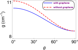
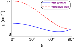
Figure 2: (Color online) Behaviour of gain amount $g$ as a function of incidence angle $\theta$ corresponding to the with and without 2D materials cases.

Fig. 3 displays how properties of 2D materials influence the gain decrement. It is immediate that adjusting parameters of 2D WSM causes the gain amount to lower considerably, even the smallest possible gain value, compared to the adjustment of graphene parameters. As for the graphene (top row), the maximum gain reduction happens at smaller temperatures and chemical potentials such that $\mu$ is less than resonance frequency at which $\mu_{res}=\hbar\omega/2$ occurs. Meanwhile, as regards to 2D WSM, the extreme gain reduction is typically obtained by decreasing the wavelength $\lambda$ and parameter $b$. It is also intriguing to observe that there is a minimum limit for the $b$ value corresponding to each wavelength, for instance, $b_{min}\approx 0.000086$ Å for $\lambda=800$ nm. In particular, $b$ values slightly greater than $b_{min}$ yield the least gain amounts, and are preferred for a better lasing effect, see [53] for the possible $b$ values of a realistic 2D WSM. Lastly, we remark that temperature (and also chemical potential) dependence of refractive indices in both cases (in particular with the graphene case) is ignored safely since it yields negligible effect (about 0.001%) within the temperature ranges of interest [54, 55].

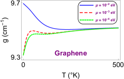
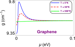
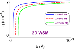
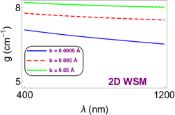
Figure 3: (Color online) Dependence of gain value on the temperature and chemical potential of graphene sheets (top row) for graphene, and parameter $b$ and wavelength $\lambda$ for 2D WSM (bottom row).

4 Broadband CPA-Laser Action with Equal Amplitude and Phase of Incoming Waves

CPA action emerges in principle when time-reversed system satisfies the self-dual spectral singularity condition given in (17) simultaneously with lasing incidence. This intriguing case is a special occasion that exists only if the correct and exact amplitudes and phases of the incoming waves are emitted from both sides of the optical system such that overlapping waves are eventually supposed to interfere destructively. In the case of CPA the waves outside are originated by an incidence angle of $-\theta$, and amplitudes of incoming waves are related to each other in terms of amplitudes given in (4) by the ratio [11]

$$\rho=\frac{a_{4}^{\ast}\,e^{-2ik_{z}L}}{b_{1}^{\ast}},$$ (22)

such that incoming waves are absorbed perfectly to build full destructive interference. In fact, $a_{4}$ can be expressed in terms of $b_{1}$ by using the spectral singularity condition. Spectral singularity condition entails $a_{1}=b_{4}=0$ such that purely outgoing waves take place. Thus, together with the boundary conditions and CPA condition in (17) one gets

$$a_{4}=\frac{e^{-2ik_{z}L}\,b_{1}}{\tilde{{\mathfrak{n}}}^{\ast}}\sqrt{\frac{V_{+}\,V_{-}^{\ast}}{\mathfrak{u}_{+}^{(2)\ast}\mathfrak{u}_{-}^{(3)\ast}}}.$$ (23)

Hence, we obtain that incoming waves are perfectly absorbed provided that $\rho$ satisfies

$$\rho=\frac{1}{\tilde{{\mathfrak{n}}}}\sqrt{\frac{V_{+}^{\ast}\,V_{-}}{\mathfrak{u}_{+}^{(2)}\mathfrak{u}_{-}^{(3)}}}.$$ (24)

Notice that one must hold incoming waves with the ratio of amplitudes $\left|\rho\right|$ and corresponding phase difference $\delta\phi$ defined by $e^{i\delta\phi}=\rho/\left|\rho\right|$ to obtain a CPA-laser. Although the attainment of $\left|\rho\right|$ and $\delta\phi$ yields a perfect CPA case, the easiest condition could be adopted by setting $\rho=1$ so that amplitudes and phases of the waves emergent outside the slab are the same. This yields

$$V_{+}^{\ast}\,V_{-}=\tilde{{\mathfrak{n}}}^{2}\,\mathfrak{u}_{+}^{(2)}\,\mathfrak{u}_{-}^{(3)}$$ (25)

This is a complex equation that gives the parameters of a CPA yielding equal amplitudes and phases of the incoming waves. An experimental realization of this fact in the case of dispersion could be expressed for both graphene and 2D WSM in Table 1, where the slab thickness is taken as $L=1$ cm, see appendix for the dispersion effect.

		with Graphene ($T=300~{}^{\circ}K$ and $\mu=5~{}\textrm{meV}$)			$-$	with 2D WSM ( $b=0.05~{}$Å)
	$\theta$	$0^{\circ}$	$-40^{\circ}$	$-80^{\circ}$		$0^{\circ}$	$-40^{\circ}$	$-80^{\circ}$
	$\lambda$	$807.996~{}\textrm{nm}$	$808.009~{}\textrm{nm}$	$807.994~{}\textrm{nm}$		$808.006~{}\textrm{nm}$	$808.001~{}\textrm{nm}$	$807.999~{}\textrm{nm}$
	$g$	$9.722~{}\textrm{cm}^{-1}$	$9.087~{}\textrm{cm}^{-1}$	$8.626~{}\textrm{cm}^{-1}$		$7.798~{}\textrm{cm}^{-1}$	$8.547~{}\textrm{cm}^{-1}$	$0.779~{}\textrm{cm}^{-1}$
	$\kappa$	$-6.251\times 10^{-5}$	$-5.843\times 10^{-5}$	$-5.546\times 10^{-5}$		$-5.014\times 10^{-5}$	$-5.496\times 10^{-5}$	$-5.011\times 10^{-6}$

Table 1: Physical parameters for the construction of a bidirectionally equal amplitude and phase CPA for various incident angles corresponding to the graphene and 2D WSM cases.

However, for the construction of a broadband CPA, we split the real and imaginary parts of (25) to obtain the following

$$\mathfrak{a}_{-}\,\cos\left(2k_{z}L\tilde{\eta}\right)-2\,\textrm{Im}[\mathfrak{u}_{+}^{(2)}]\,\sin\left(2k_{z}L\tilde{\eta}\right)=\mathfrak{c}_{1}$$ (26)

$$2\,\textrm{Im}[\mathfrak{u}_{+}^{(2)}]\,\cos\left(2k_{z}L\tilde{\eta}\right)+\mathfrak{a}_{-}\,\sin\left(2k_{z}L\tilde{\eta}\right)+\frac{\tilde{\kappa}}{\tilde{\eta}}\Bigl{\{}\mathfrak{b}_{-}\,e^{\tilde{g}L}-\mathfrak{b}_{+}\,e^{-\tilde{g}L}\Bigr{\}}=\mathfrak{c}_{2}$$ (27)

where we identified

$$\mathfrak{a}_{\pm}:=\left|\sigma^{(\ell)}+\tilde{{\mathfrak{n}}}\right|^{2}\pm 1,~{}~{}~{}\mathfrak{b}_{\pm}:=\mathfrak{a}_{+}\pm 2\left[\tilde{\eta}+\textrm{Re}[\sigma^{(\ell)}]\right],~{}~{}~{}\tilde{g}:=\frac{\eta\,g}{\sqrt{\eta^{2}-\sin^{2}\theta}}$$

$$\mathfrak{c}_{1}:=\frac{1}{4}\left\{\tilde{\eta}^{2}-1-\left|\sigma^{(\ell)}\right|^{2}-2\,\textrm{Re}[\sigma^{(\ell)}]-4\tilde{\kappa}\,\textrm{Im}[\sigma^{(\ell)}]\right\}$$

$$\mathfrak{c}_{2}:=\frac{1}{2}\left\{\tilde{\kappa}(1-\tilde{\eta})-\tilde{\eta}\,\textrm{Im}[\sigma^{(\ell)}]+\frac{\tilde{\kappa}}{\tilde{\eta}}\left[1+\left|\sigma^{(\ell)}\right|^{2}+(2+\tilde{\eta})\,\textrm{Re}[\sigma^{(\ell)}]\right]\right\}$$

Notice that the first equation (26) leads to an expression for $k$

$$k=\frac{m\pi}{\tilde{\eta}L\cos\theta}-\frac{1}{2\tilde{\eta}L\cos\theta}\sin^{-1}\left\{\frac{2\,\textrm{Im}[\mathfrak{u}_{+}^{(2)}]\mathfrak{c}_{1}-\mathfrak{a}_{-}\sqrt{\mathfrak{a}_{-}^{2}+4\textrm{Im}[\mathfrak{u}_{+}^{(2)}]^{2}-\mathfrak{c}_{1}^{2}}}{\left[\mathfrak{a}_{-}^{2}+4\textrm{Im}[\mathfrak{u}_{+}^{(2)}]^{2}\right]}\right\}$$ (28)

where $m$ is the mode number that corresponds to the CPA points obtained by means of self-dual spectral singularity condition in (17). We observe that in fact when all other parameters are kept fixed, the wavelength $\lambda$ is inversely proportional to the mode number $m$ according to (28). Thus, for each $m$, the wavelength becomes unique. If the mode number is large enough so that self-dual spectral singularity points seem to behave as continuous, one can speak of broadband CPA phenomenon. Hence, it is easy to show that broadband range of a CPA realization is computed as

$$\Delta\lambda=\frac{\lambda^{2}\left|\Delta m\right|}{2L\tilde{\eta}\cos\theta},$$ (29)

where $\lambda$ corresponds to wavelength at the center of interval $\Delta\lambda$ which could be computed via (28). Fig. 4 serves as the pictorial demonstration of this situation, which is associated with graphene in the left board and 2D WSM in the right board. For the purpose of realizing the broadband CPA, we employ a wide slab thickness of 10 cm in size with the wave emergent by angle $\theta=-30^{\circ}$. In the case of graphene, provided that self-dual spectral singularity condition gives rise to the mode number $m=331106$ corresponding to the wavelength $\lambda=1056.992$ nm, and the gain amount $g\approx 3734~{}\textrm{cm}^{-1}$ with the graphene features of $T=300^{\circ}\textrm{K}$ and $\mu=0.005~{}\textrm{eV}$ for the chemical potential, one obtains broadband CPA with $\Delta\lambda_{g}=0.1$ nm corresponding to the wavelength range (1055.75 nm, 1055.85 nm). Likewise, for the 2D WSM, one obtains $m=331107$, $\lambda=1057.145$ nm, $g\approx 3211~{}\textrm{cm}^{-1}$, and parameter $b=0.05$ Å to obtain $\Delta\lambda_{w}=6$ nm corresponding to the wavelength range (1055 nm, 1061 nm) within $1\%$ of precision. This shows that the expression (29) yields quite well estimation of broadband CPA condition once the self-dual spectral singularity points are determined corresponding to a mode number $m$. Also, the use of 2D WSM is favorable for the realization of broadband CPA due to its nice features present in its conductivity expression. We stress out that this broadband structure perfectly fits an intriguing situation of equal amplitude and phase conditions of the particular CPA provided. Finally, we realize that Eq. 27 enables to compute the necessary gain amount corresponding to equal amplitude and phase conditions, which verifies the results obtained in Figs. 2 and 3.

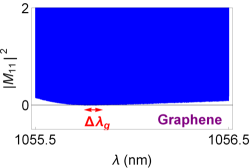
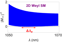
Figure 4: (Color online) Broadband CPA for the case of graphene and 2D WSM. $\Delta\lambda_{g}=0.1$ nm corresponding to the range (1055.75 nm, 1055.85 nm) and $\Delta\lambda_{w}=6$ nm corresponding to the range (1055 nm, 1061 nm) give rise to the broadband CPA within $1\%$ of flexibility.

5 Concluding Remarks

In this study, we provide necessary conditions to obtain equal wave amplitudes and phases corresponding to a $\mathcal{PT}$-symmetric CPA system which is covered by 2D materials. We impose an overall $\mathcal{PT}$ symmetry in the system just because of the symmetry conditions arising from duality between the lasing and CPA phenomena. We derived exact expression for the CPA condition based on the particular 2D materials in (17). Although our expression in (17) holds for all 2D materials with scalar-valued conductivities, we in particular employed graphene and 2D WSM in our analysis because of their prominent roles in recent 2D materials research.

We observe that 2D WSM is much more effective than graphene in the sense of gain decrement. In particular, adjusting minimum $b$ value in 2D WSM gives rise to an incredibly low gain values. Nevertheless, In the case of graphene the gain reduction remains limited. Thus, 2D WSM is more appropriate for the construction of a good CPA. We find out that graphene is more efficient at lower temperatures and chemical potentials below the resonance conditions. However, 2D WSM is much operative around critical $b$ values at which it yields zero gain value. As the wavelength increases, efficiency of CPA-laser corresponding to 2D WSM improves.

Finally, we explicitly demonstrate necessary conditions to realize a CPA which will be formed by equal amplitudes and phases of the waves emergent from both sides. This is important because the main problem in experimental realization of a CPA is just to adjust correct amplitudes and phases of incoming waves. But our model rigorously resolves this complication. If the CPA parameters are tuned in according to (25), then any equal wave amplitudes and phases fulfils a CPA-laser. We present some exact parameters in Table 1 to guide the experimental attempts for the realization of the $\mathcal{PT}$-symmetric CPA phenomenon with 2D materials. We also present conditions for the realization of a broadband CPA in (29) which occurs at large mode numbers $m$. For this to happen, one should pick a wider slab thickness $L$ such that corresponding self-dual spectral singularity points give rise to relatively high $m$ values. Although our model is focused on two representative 2D material types, it comprehends set of all 2D materials whose conductivities should be given with corresponding parameters. Novelty of our results awaits experimental verification which is significant to establish a realistic CPA, and to address the direction of research accordingly.

Appendix A Dispersion Effect

If there exists a dispersion in the refractive index ${\mathfrak{n}}$, then we need to incorporate the effect of wavenumber $k$ on ${\mathfrak{n}}$. We imagine that active part of the optical system composing the gain ingredient is formed by doping a host medium of refractive index $n_{0}$, and its refractive index satisfies the dispersion relation

$${\mathfrak{n}}^{2}=n_{0}^{2}-\frac{\hat{\omega}_{p}^{2}}{\hat{\omega}^{2}-1+i\hat{\gamma}\,\hat{\omega}},$$ (30)

where $\hat{\omega}:=\omega/\omega_{0}$, $\hat{\gamma}:=\gamma/\omega_{0}$, $\hat{\omega}_{p}:=\omega_{p}/\omega_{0}$, $\omega_{0}$ is the resonance frequency, $\gamma$ is the damping coefficient, and $\omega_{p}$ is the plasma frequency. The $\hat{\omega}_{p}^{2}$ can be described in leading order of the imaginary part $\kappa_{0}$ of ${\mathfrak{n}}$ at the resonance wavelength $\lambda_{0}:=2\pi c/\omega_{0}$ by the expression $\hat{\omega}_{p}^{2}=2n_{0}\hat{\gamma}\kappa_{0}$, where quadratic and higher order terms in $\kappa_{0}$ are ignored [56]. We replace this equation in (30), employ the first expression of (19) and neglecting quadratic and higher order terms in $\kappa_{0}$, we obtain the real and imaginary parts of refractive index as follows [21, 22, 23, 24, 56]

$$\eta\approx n_{0}+\frac{\kappa_{0}\hat{\gamma}(1-\hat{\omega}^{2})}{(1-\hat{\omega}^{2})^{2}+\hat{\gamma}^{2}\hat{\omega}^{2}},\qquad\kappa\approx\frac{\kappa_{0}\hat{\gamma}^{2}\hat{\omega}}{(1-\hat{\omega}^{2})^{2}+\hat{\gamma}^{2}\hat{\omega}^{2}}.$$ (31)

$\kappa_{0}$ can be written as $\kappa_{0}=-\lambda_{0}g_{0}/4\pi$ at resonance wavelength $\lambda_{0}$, see (21). Substituting this relation in (31) and making use of (19) and (25), we can determine $\lambda$ and $g_{0}$ values for the CPA with equal amplitudes and phases yielding a perfect destructive interference. These are explicitly calculated for various parameters in Table 1 for our setup of the $\mathcal{P}\mathcal{T}$-symmetric bilayer covered by 2D materials. Furthermore, Nd:YAG crystals forming the slab material hold the following $\hat{\gamma}$ value corresponding to the related refractive index and resonance wavelength [57]:

$$n_{0}=1.8217,\qquad\lambda_{0}=808\,{\rm nm},\hat{\gamma}=0.003094.$$ (32)

References

- [1] Y. D. Chong, L. Ge, H. Cao, and A. D. Stone, Phys. Rev. Lett. 105, 053901 (2010).
- [2] S. Longhi, Physics 3, 61 (2010).
- [3] S. Longhi, Phys. Rev. A 82, 031801 (2010).
- [4] S. Longhi, Phys. Rev. A 83, 055804 (2011).
- [5] S. Longhi, Phys. Rev. Lett. 107, 033901 (2011).
- [6] W. Wan, Y. Chong, L. Ge, H. Noh, A. D. Stone, and H. Cao, Science 331, 889 (2011).
- [7] L. Ge, Y. D. Chong, S. Rotter, H. E. Türeci, and A. D. Stone, Phys. Rev. A 84, 023820 (2011).
- [8] D. G. Baranov, A. E. Krasnok, T. Shegai, A. Alù, and Y. D. Chong, Nature Reviews Materials 2, 17064 (2017).
- [9] T. Roger, S. Vezzoli, E. Bolduc, J. Valente, J. J. F. Heitz, J. Jeffers, C. Soci, J. Leach, C. Couteau, N. I. Zheludev and D. Faccio, Nat. Commun. 6, 7031 (2015).
- [10] H. Ramezani, Y. Wang, E. Yablonovitch, and X. Zhang, IEEE J. Sel. Top. Quantum Electron. 22, 115 (2016).
- [11] A. Mostafazadeh and M. Sarısaman, Ann. Phys. (NY) 375, 265-287 (2016).
- [12] A. Mostafazadeh, J. Phys. A 45, 444024 (2012).
- [13] M. A. Naimark, Trudy Moscov. Mat. Obsc. 3, 181 (1954) in Russian, English translation: Amer. Math. Soc. Transl. (2), 16, 103 (1960).
- [14] G. Sh. Guseinov, Pramana J. Phys. 73, 587 (2009).
- [15] A. Mostafazadeh and H. Mehri-Dehnavi, J. Phys. A 42, 125303 (2009).
- [16] C. M. Bender and S. Boettcher, Phys. Rev. Lett. 80 5243, (1998).
- [17] K. G. Makris, R. El-Ganainy, D. N. Christodoulides, and Z. H. Musslimani, Phys. Rev. Lett. 100 103904, (2008).
- [18] C. E. Rüter, K. G. Makris, R. El-Ganainy, D. N. Christodoulides, M. Segev, and D. Kip, Nat. Phys. 6 192, (2010).
- [19] A. Mostafazadeh, Geometric Methods in Physics, Trends in Mathematics, edited by P. Kielanowski, P. Bieliavsky, A. Odzijewicz, M. Schlichenmaier, and T. Voronov (Springer, Cham, 2015) pp 145-165; arXiv: 1412.0454.
- [20] S. Longhi, Phys. Rev. A 82, 032111 (2010).
- [21] A. Mostafazadeh, M. Sarisaman, Phys. Lett. A 375, 3387 (2011).
- [22] A. Mostafazadeh, M. Sarisaman, Proc. R. Soc. Lond. Ser. A Math. Phys. Eng. Sci. 468, 3224 (2012).
- [23] A. Mostafazadeh, M. Sarisaman, Phys. Rev. A 87, 063834 (2013).
- [24] A. Mostafazadeh, M. Sarisaman, Phys. Rev. A 88, 033810 (2013).
- [25] A. Mostafazadeh and M. Sarısaman, Phys. Rev. A 91, 043804 (2015).
- [26] C. Yan, M. Pu, J. Luo, Y. Huang, X. Li, X. Ma, X. Luo, Opt. Laser Technol. 101, 499 (2018).
- [27] L. Feng, Y. L. Xu, W. S. Fegadolli, M. H. Lu, J. E. Oliveira, V. R. Almeida, Y. F. Chen, A. Scherer, Nat. Mater. 12, 108 (2013).
- [28] Y. Shen, X. Hua Deng, and L. Chen, Opt. Express 22, 19440 (2014).
- [29] M. Sarısaman, Phys. Rev. A 95, 013806 (2017).
- [30] M. Sarısaman, M. Tas, Phys. Rev. B 97, 045409 (2018).
- [31] T. Smolenski, T. Kazimierczuk, M. Goryca, M. R. Molas, K. Nogajewski, C. Faugeras, M. Potemski and P. Kossacki, 2D Mater. 5, 015023 (2018).
- [32] F. Schedin, A. K. Geim, S. V. Morozov, E. W. Hill, P. Blake, M. I. Katsnelson, and K. S. Novoselov, Nat. Mater. 6, 652 (2007).
- [33] R. Stine, J. T. Robinson, P. E. Sheehan, and Cy R. Tamanaha, Adv. Mater. 22, 5297 (2010).
- [34] Q. He, S. Wu, Z. Yin, and H. Zhang, Chem. Sci. 3, 1764 (2012).
- [35] J. Duffy, J. Lawlor, C. Lewenkopf, and M. S. Ferreira, Phys. Rev. B 94, 045417 (2016).
- [36] S. Chen, Z. Han, M. M. Elahi, K. M. M. Habib, L. Wang, B. Wen, Y. Gao, T. Taniguchi, K. Watanabe, J. Hone, A. W. Ghosh, and C. R. Dean, Science 353, 1522 (2016).
- [37] P. -Y. Chen and A. Alu, ACS Nano 5, 5855 (2011).
- [38] M. Danaeifar and N. Granpayeh, J. Opt. Soc. Am. B 33, 1764 (2016).
- [39] M. Naserpour, C. J. Zapata-Rodríguez, S. M. Vuković, H. Pashaeiadl and M. R. Belić, Sci. Rep. 7, 12186 (2017).
- [40] D. Jariwala, T. Marks, M. Hersam, Nat. Mater. 16, 155 (2017).
- [41] A. Gupta, T. Sakthivel and S. Seal, Prog. Mater. Sci. 73, 44 (2015).
- [42] A. Molle, J. Goldberger, M. Houssa, Y. Xu, S. C. Zhang and D. Akinwande, Nat. Mater. 16, 163 (2017).
- [43] S. Zanotto, F. Bianco, V. Miseikis, D. Convertino, C. Coletti, and A. Tredicucci, APL Photonics 2, 016101 (2017).
- [44] F. Liu, Y. D. Chong, S. Adam, and M. Polini, 2D Mater. 1, 031001 (2014).
- [45] Y. Fan, F. Zhang, Q. Zhao, Z. Wei, and H. Li, Opt. Lett. 38, 6269 (2014).
- [46] S. M. Rao, J. J. F. Heitz, T. Roger, N. Westerberg, and D. Faccio, Opt. Lett. 39, 5345 (2014).
- [47] Y. Fan, Z. Liu, F. Zhang, Q. Zhao, Q. Fu, J. Li, C. Gu, and H. Li, Sci. Rep. 5, 13956 (2015).
- [48] A. Mostafazadeh, Phys. Rev. Lett. 102, 220402 (2009).
- [49] B. Wunsch, T. Stauber, F. Sols and F. Guinea, New J. Phys. 8, 318 (2006).
- [50] E. H. Hwang and S. Das Sarma, Phys. Rev. B 75, 205418 (2007).
- [51] L. A. Falkovsky, Physics-Uspekhi 51, 887 (2008).
- [52] M. Kargarian, M. Randeria, and N. Trivedi, Sci. Rep. 5, 12683 (2015).
- [53] Q. Ma, S. Xu, C. Chan, C. Zhang, G. Chang, Y. Lin, W. Xie, T. Palacios, H. Lin, S. Jia, P. A. Lee, P. Jarillo-Herrero and N. Gedik, Nat. Phys. 13, 842 (2017).
- [54] T. Y. Fan, J. L. Daneu, Applied Optics 37, 1635 (1998).
- [55] M. Bertolotti, V. Bogdanov, A. Ferrari, A. Jascow, N. Nazorova, A. Pikhtin, L. Schirone, J. Opt. Soc. Am. B 7, 918 (1990).
- [56] A. Mostafazadeh, Phys. Rev. A 83, 045801 (2011).
- [57] W. T. Silfvast, Laser Fundamentals, Cambridge University Press, Cambridge, 1996.