Evidence of Systematic Errors in Spitzer Microlens Parallax Measurements

Abstract

The microlensing parallax campaign with the Spitzer space telescope aims to measure masses and distances of microlensing events seen towards the Galactic bulge, with a focus on planetary microlensing events. The hope is to measure how the distribution of planets depends on position within the Galaxy. In this paper, we compare 50 microlens parallax measurements from the 2015 Spitzer campaign to three different Galactic models commonly used in microlensing analyses, and we find that $\geq 74\,$% of these events have microlensing parallax values higher than the medians predicted by Galactic models. The Anderson-Darling tests indicate probabilities of $p_{\rm AD}<6.6\times 10^{-5}$ for these three Galactic models, while the binomial probability of such a large fraction of large microlensing parallax values is $<4.6\times 10^{-4}$. Given that many Spitzer light curves show evidence of large correlated errors, we conclude that this discrepancy is probably due to systematic errors in the Spitzer photometry. We find formally acceptable probabilities of $p_{\rm AD}>0.05$ for subsamples of events with bright source stars ($I_{\rm S}\leq 17.75$) or Spitzer coverage of the light curve peak. This indicates that the systematic errors have a more serious influence on faint events, especially when the light curve peak is not covered by Spitzer. We find that multiplying an error bar renormalization factor of 2.2 by the reported error bars on the Spitzer microlensing parallax measurements provides reasonable agreement with all three Galactic models. However, corrections to the uncertainties in the Spitzer photometry itself are a more effective way to address the systematic errors.

1 Introduction

The gravitational microlensing method (Mao & Paczynski, 1991) is sensitive to planetary systems at any distance between the Sun and the Galactic center. While distant planets can also be detected by the transit method, microlensing is probably the best method to measure the planet distribution in our galaxy. A study of the Galactic distribution of planets can reveal the history of planet formation in our galaxy and the mechanism of planet formation in the Galactic bulge, which has a much higher density of stars than the Solar neighborhood. Thus far, Penny et al. (2016) attempt a comparison of the distribution of distances to planetary microlens systems with expectations based on a galactic model. One aspect of the microlensing method which makes such a statistical study difficult is that the lens mass $M_{L}$ and distance $D_{L}$ are not uniquely determined for most microlensing events.

To directly measure the lens mass, $M_{L}$, and estimate the distance, $D_{L}$, both the angular Einstein radius, $\theta_{\rm E}$, and the microlens parallax $\pi_{\rm E}$ must be measured. The angular Einstein radius, $\theta_{\rm E}$, is given by

$$\theta_{\rm E}\equiv\sqrt{\kappa M_{L}\pi_{\rm rel}}\ ,$$ (1)

where $\kappa=8.144~{}{\rm mas}~{}M_{\odot}^{-1}$, $\pi_{\rm rel}={\rm 1\,AU}(D_{L}^{-1}-D_{S}^{-1})$ and $D_{S}$ is the distance to the source star, which is approximately 8 kpc. The microlens parallax, $\pi_{\rm E}$, is given by

$$\pi_{\rm E}\equiv\frac{\pi_{\rm rel}}{\theta_{\rm E}}\ ,$$ (2)

and the lens mass can be obtained by eliminating $\pi_{\rm rel}$ from equations 1 and 2 to yield

$$M_{L}={\theta_{\rm E}\over\kappa\pi_{\rm E}}\ .$$ (3)

The angular Einstein radius can be measured when the finite source effect is seen in the light curve or when the lens-source separation is measured after the microlensing event (Bennett et al., 2015; Batista et al., 2015; Bhattacharya et al., 2018). Microlensing parallax, $\pi_{\rm E}$, has traditionally been measured via the detection of the effects of the Earth’s orbital motion in the light curve (Alcock et al., 1995; An et al., 2002; Muraki et al., 2011). Because these two effects are only occasionally measured, the only light curve parameter that constrains the lens mass and distance is Einstein radius crossing time,

$$t_{\rm E}\equiv\frac{\theta_{\rm E}}{\mu_{\rm rel}}\ ,$$ (4)

where $\mu_{\rm rel}$ is the lens-source relative proper motion. For planetary events, the angular Einstein radius $\theta_{\rm E}$ is commonly measured because planetary events usually show finite source effects, but the orbital microlensing parallax effect is detected only when the event’s Einstein radius crossing time is relatively long. As a result, only $\sim 20\%$ planetary events have their mass and distance determined by the combination of $\theta_{\rm E}$ and $\pi_{\rm E}$ (e.g., Bennett et al., 2010; Muraki et al., 2011). For events where the finite source effect and/or the orbital parallax effect were not measured, probability distributions for the lens mass and distance can be estimated with a Bayesian analysis using the Galactic model as its prior probability distribution, under the assumption that the planet hosting probability does not depend on the lens mass and distance (e.g., Beaulieu et al., 2006; Bennett et al., 2014). It is also possible to determine the mass and distance of the lens system by combining high angular resolution follow-up observations with adaptive optics (AO) or the Hubble Space Telescope (HST) and mass luminosity relations (Batista et al., 2015; Bennett et al., 2015; Koshimoto et al., 2017a, b; Bhattacharya et al., 2018). However, these observations must be taken several years after the event to measure the lens-source separation, depending on the $\mu_{\rm rel}$ value.

One might think of a statistical study of events with measurements of orbital microlensing parallax effects to determine the Galactic distribution of planets, but unfortunately, orbital microlensing parallax is difficult to detect for systems more distant than $D_{L}\approx 4\,$kpc (Sumi et al., 2016; Bennett et al., 2018a). Penny et al. (2016) did attempt to compare the planetary occurrence rate as a function of $D_{L}$, but this attempt was plagued by an inhomogeneous sample, incorrect parallax measurements (Han et al., 2016), and overly optimistic detection efficiency estimates.

A more serious attempt to measure the Galactic distribution of planetary systems has been made with the Spitzer microlensing campaign (Yee et al., 2015a; Udalski et al., 2015), which is a systematic program to make $\pi_{\rm E}$ measurements of microlensing events identified by ground-based surveys since 2014. This program makes use of the $\sim 1\,$AU separation between Spitzer and the Earth, to measure $\pi_{\rm E}$ for a carefully selected sample of events. Zhu et al. (2017) did a statistical analysis of the 2015 Spitzer campaign, and they estimated that $\sim 1/3$ of all planet detections from the Spitzer campaign should be located in the bulge if the planet distributions are the same in the bulge as in the disk.

However, there are correlated systematic errors in many of the Spitzer light curves (Poleski et al., 2016; Zhu et al., 2017), and they can potentially affect the microlensing parallax measurements. Zhu et al. (2017) also discuss this. In particular, they describe that prominent deviations from single lens model, caused by the unknown systematics, are seen in the Spitzer light curves for 5 events out of their raw sample of 50 events (see section 5.1 of their paper). In a handful of events the Spitzer microlensing parallax measurements are consistent with a ground based parallax measurements (Udalski et al., 2015; Poleski et al., 2016; Han et al., 2017; Shin et al., 2017; Wang et al., 2017). Also, some previous studies conducted tests on much smaller samples of published events with Spitzer parallax measurements that might possibly be reinterpreted as tests of consistency between the measurements and the Galactic model. Shan et al. (2019) considered a non-statistical sample of 13 published microlensing events with measurements of $\theta_{\rm E}$ and $\pi_{\rm E}$ from Spitzer that are considered to be secure. They then compare the Bayesian predictions for the lens system mass and distance to the results from Spitzer $\pi_{\rm E}$ measurements. Zang et al. (2020) consider a sample of 8 published single-lens events without taking into account “detection efficiency, and possible selection or publication biases.” So, both of these samples consist of events that the Spitzer team selected to publish because they were considered to be “interesting”, which results in publication bias. Most of the events in these samples have a bright source star or a good Spitzer light curve coverage over the peak or a caustic crossing. So, they have much stronger signals in the Spitzer data than is typical. The published events are also less likely to have the obvious systematic photometry errors than a systematically selected statistical sample. Therefore, these comparisons are not precise enough to provide a useful test of the precision of typical Spitzer microlensing parallax measurements. There are many events for which the Spitzer light curve data have poor coverage of both the magnified portion of the light curve and the baseline. These events might well have large systematic errors in the $\pi_{\rm E}$ measurements due to systematic errors in the Spitzer photometry. Also, three microlensing events have been interpreted as lens systems located in the Galactic disk that are orbiting perpendicular to or in the opposite direction of disk rotation based on Spitzer data with poor light curve coverage (Shvartzvald et al., 2017, 2019; Chung et al., 2019). The prior probability for such orbits is quite low ($\lower 2.15277pt\hbox{$\;\buildrel<\over{\sim}\;$}10^{-3}$), so it seems quite possible that the microlensing parallax signals for these events are spurious due to systematic Spitzer photometry errors.

In this paper, we compare the measurements of $t_{\rm E}$ and $\pi_{\rm E}$ for the sample of 50 single lens events from the 2015 Spitzer data (Zhu et al., 2017), to the predicted distributions based on Galactic models. We consider three different Galactic models previously used for microlensing studies, including the one used by Zhu et al. (2017). We use a Bayesian analysis to compute the posterior distribution for the parallax measurement $f_{\rm post}(\pi_{\rm E})$ for each event in the sample. We then compare the medians, $\widetilde{\pi}_{\rm E,post}$, of these $\pi_{\rm E}$ posteriors to the predictions of the three Galactic models, and use the binomial distribution to show that the distribution of $\widetilde{\pi}_{\rm E,post}$ values in inconsistent with the Galactic models. In order to explore this comparison in more detail, we convert each posterior $f_{\rm post}(\pi_{\rm E})$ distribution into a distribution called the posterior inverse percentile distribution, and we compare the cumulative density function (CDF) of inverse percentile to the theoretical distribution using the Anderson-Darling (AD) test. This indicates the null hypothesis that the observed distribution follows the model is rejected at high significance, $p_{\rm AD}\leq 6.6\times 10^{-5}$, for all three of the Galactic models that we consider. We also conduct these same tests for several sub-samples and find formally acceptable probabilities of $p_{\rm AD}>0.05$ for a sub-sample of 17 events with bright source stars of $I_{\rm S}<17.75$ and for a different 20 events sub-sample with the light curve peak covered by Spitzer. However, for sub-samples with fainter source stars or without Spitzer light curve coverage of the peak or caustic crossing, the probability is dramatically smaller. We interpret this as evidence that the measured ${\mbox{\boldmath$\bf\pi$}_{\rm E,obs}}$ are contaminated by the systematic photometry errors in the Spitzer data, especially for faint events and events without Spitzer light curve peak coverage.

This paper is organized as follows. In Section 2 we explain our method, focusing the basic idea on how we compare observations with a model without calculating detection efficiencies. We explain the three Galactic models that we employ (Zhu et al., 2017; Sumi et al., 2011; Bennett et al., 2014) and focus on the differences between these models in Section 3. In Section 4, we explain the Zhu et al. (2017) sample and how we derive the posterior $\pi_{\rm E}$ distribution for each event. Section 5 presents the results of our statistical comparison between the posterior and the model predicted $\pi_{\rm E}$ distributions using the Anderson-Darling (AD) statistics. We present the same statistical tests with modified Galactic models in Section 6, and we show that reasonable Galactic model modifications cannot explain the Spitzer measurements. In the same section, we also discuss other potential factors that might possibly affect the results, and we show the discrepancy cannot be explained by these factors. We discuss Spitzer systematic photometry errors in Section 7, and we describe our findings of correlations between the level of systematic errors in the $\pi_{\rm E}$ distribution and the source brightness and Spitzer signal strength. We present our conclusions in Section 8.

2 Method

One of general difficulties involved in the comparison of an observational data set with a model is the determination of detection efficiencies (or selection effects). The detection efficiency is defined as the probability that a microlensing event is selected to be part of the sample being studied. The seven parameters that characterize a single lens are: the time of closest angular approach between the source and lens stars, $t_{0}$, the impact parameter of the source trajectory with respect to the lens star, $u_{0}$, the Einstein radius crossing time, $t_{\rm E}$, the angular Einstein radius, $\theta_{\rm E}$, the microlens parallax vector, ${\bm{\pi}_{\rm E}}=\pi_{\rm E}\,{\bm{\mu}_{\rm rel}}/\mu_{\rm rel}=(\pi_{\rm E,N},\pi_{\rm E,E})$, and the source flux $F_{\rm S}$. The microlensing parallax vector, ${\bm{\pi}_{\rm E}}$, is a vector with a magnitude of $\pi_{\rm E}$ and a direction parallel to ${\bm{\mu}_{\rm rel}}$. The north and east components are $\pi_{\rm E,N}$ and $\pi_{\rm E,E}$, respectively (Gould, 1992). Four of these parameters affect the detection efficiency of an event; $t_{0}$ determines the coverage of the light curve; $u_{0}$ determines the peak magnification; $t_{\rm E}$ is the event duration, and $F_{\rm S}$ controls the brightness and photometric signal to noise ratio. The parameters that provide information about the lens mass and the distance to the lens are $t_{\rm E}$, $\theta_{\rm E}$ and $\pi_{\rm E}$. Therefore, the probability (density) for a single lens event to occur, be discovered, and then be selected to be part of the sample being studied can be decomposed into three other functions,

$$f_{\rm obs}(t_{\rm E},\theta_{\rm E},{\bm{\pi}_{\rm E}},t_{0},u_{0},F_{\rm S})\propto\Gamma_{\rm Gal}(t_{\rm E},\theta_{\rm E},{\bm{\pi}_{\rm E}})\,\eta(t_{0},u_{0},F_{\rm S})\,\epsilon(t_{\rm E},t_{0},u_{0},F_{\rm S})\ ,$$ (5)

where $\Gamma_{\rm Gal}(t_{\rm E},\theta_{\rm E},{\bm{\pi}_{\rm E}})$ is the event rate of a microlensing event with parameters $(t_{\rm E},\theta_{\rm E},{\bm{\pi}_{\rm E}})$, and $\eta(t_{0},u_{0},F_{\rm S})$ is proportional to the probability distribution of these three parameters that are independent of $t_{\rm E}$, $\theta_{\rm E}$ and ${\bm{\pi}_{\rm E}}$. The detection efficiency is given by $\epsilon(t_{\rm E},t_{0},u_{0},F_{\rm S})$, and it is effectively independent of $\theta_{\rm E}$ and ${\bm{\pi}_{\rm E}}$ for the events in the Spitzer sample. Note that in other contexts (e.g., Suzuki et al., 2016) it is common to average over the dependence of $\epsilon$ on $t_{0}$, $u_{0}$, and $F_{\rm S}$, but for this analysis we consider a specific sample of events for which these parameters have been measured.

If we want to compare an observed Einstein radius crossing time ($t_{\rm E}$) distribution with the predictions from Galactic models, we need to calculate the average detection efficiency as a function of $t_{\rm E}$ by simulating event detection processes using artificial events (Alcock et al., 1996, 1997, 2000a, 2000b; Sumi et al., 2003, 2011; Mróz et al., 2017). However, our interest here is not in the $t_{\rm E}$ distribution, but in the $\pi_{\rm E}$ distribution which is obtained by the Spitzer microlensing parallax measurements. In this case, we can compare the observed $\pi_{\rm E}$ distribution with the model-predicted distribution without any calculation of the detection efficiencies. When we consider a specific event with observed parameters $(t_{\rm E},t_{0},u_{0},F_{\rm S})=(t_{\rm E,obs},t_{\rm 0,obs},u_{\rm 0,obs},F_{\rm S,obs})$, the probability distribution for $\theta_{\rm E}$ and ${\bm{\pi}_{\rm E}}$ is given by

$$f_{\rm obs}(\theta_{\rm E},{\bm{\pi}_{\rm E}}\,|\,t_{\rm E,obs},t_{\rm 0,obs},u_{\rm 0,obs},F_{\rm S,obs}) = \frac{f_{\rm obs}(t_{\rm E,obs},\theta_{\rm E},{\bm{\pi}_{\rm E}},t_{\rm 0,obs},u_{\rm 0,obs},F_{\rm S,obs})}{f_{\rm obs}(t_{\rm E,obs},t_{\rm 0,obs},u_{\rm 0,obs},F_{\rm S,obs})}$$ (6)

$$\propto \Gamma_{\rm Gal}(\theta_{\rm E},{\bm{\pi}_{\rm E}}\,|\,t_{\rm E,obs})\ ,$$

since we are considering the case of fixed $t_{\rm E}$, $t_{0}$, $u_{0}$, and $F_{\rm S}$ at the observed values. We have defined the probability density distribution $f(A\,|\,B)$ to be the conditional probability density distribution for $A$ given $B$, and generally $f(A\,|\,B)=f(A,B)/f(B)$. In other words, $\Gamma_{\rm Gal}(\theta_{\rm E},{\bm{\pi}_{\rm E}}\,|\,t_{\rm E})$ is the probability distribution of $\theta_{\rm E}$ and ${\bm{\pi}_{\rm E}}$ for events with a given $t_{\rm E}$ value. We calculate this probability using the Galactic model. In Eq. (6), the detection efficiency factor is canceled because the values of $\theta_{\rm E}$ and ${\bm{\pi}_{\rm E}}$ are completely independent of $t_{\rm 0,obs}$ and $u_{\rm 0,obs}$. We show below in Section 6.2 that our results do not depend on the weak dependence of $\theta_{\rm E}$ and ${\bm{\pi}_{\rm E}}$ on $F_{\rm S,obs}$. The remaining parameter that depends on $\epsilon(t_{\rm E},t_{0},u_{0},F_{\rm S})$ is $t_{\rm E}$, but this is fixed to be $t_{\rm E,obs}$ in Eq. (6), so we don’t need to use the detection efficiency here. This equation indicates that the observed distribution can be directly compared with the Galactic model.

Because the angular Einstein radius $\theta_{\rm E}$ is not measured for most of the Spitzer events, we focus on the magnitude of microlens parallax $\pi_{\rm E}$ measured by the Spitzer campaign. In this case, the equation

$$f_{\rm obs}(\pi_{\rm E}\,|\,t_{\rm E,obs},t_{\rm 0,obs},u_{\rm 0,obs},F_{\rm S,obs})\propto\Gamma_{\rm Gal}(\pi_{\rm E}\,|\,t_{\rm E,obs})$$ (7)

is still true because of the same logic. We use the Galactic models explained in Section 3 as the right-hand side of the model-predicted $\pi_{\rm E}$ distribution. For the left-hand side of observational $\pi_{\rm E}$ distribution, we use the posterior $\pi_{\rm E}$ distribution obtained by combining the Galactic prior with the raw sample 50 events of Zhu et al. (2017), which are described in Section 4. Note that our choice of focusing on the 1D distribution of $\pi_{\rm E}$ rather than the 2D distribution of $\pi_{\rm E,N}$ and $\pi_{\rm E,E}$ is because there is no well-established statistical test to compare 2D distributions as long as we know. Using only 1D distribution makes our results more conservative.

3 Models

To calculate $\Gamma_{\rm Gal}(\pi_{\rm E}\,|\,t_{\rm E,obs})$, we need a Galactic model, which consists of the stellar mass function, stellar density distribution, and velocity distribution in our galaxy. Microlensing groups have developed a number of such models, and they are often referred to as “standard Galactic model” (Sumi et al., 2011; Bennett et al., 2014; Zhu et al., 2017; Mróz et al., 2017; Jung et al., 2018). We use the model presented by Zhu et al. (2017) in the paper that presented this Spitzer sample, as well as Galactic models presented by Sumi et al. (2011) and Bennett et al. (2014) for our comparison with this Spitzer microlensing parallax sample. Hereafter we refer to these papers as and models as Z17, S11 and B14, respectively.

The Z17 and S11 models are based on the Galactic model developed by Han & Gould (1995), while the B14 model is based on the Galactic model developed by Robin et al. (2003) and it includes a central hole in the disk that was created by the disk instability thought to have formed the central Galactic bar, as well as bar rotation. The B14 model also includes a thick disk and spheroid, but none of these features are considered in Han & Gould (1995). In this section we give the outline of these three models focusing on the differences between them. We summarize them in Table 1. More details are found in each paper and references therein.

Table 1: Summary of the three Galactic models used in this work.

	Model	Z17	S11	B14
Stellar	Initial Mass function	Eq. (8)	Eq. (8)	Eq. (8)
population	$(\alpha_{\rm hm},\alpha_{\rm ms},\alpha_{\rm bd})$	(2.3, 1.3, 0.3)	(2.0, 1.3, 0.5)	(2.0, 1.3, 0.5)
	$(M_{\rm max},M_{1},M_{2},M_{\rm min})~{}[M_{\odot}]$	$(8.0,0.50,0.08,10^{-5})$	$(8.0,0.70,0.08,10^{-5})$	$(8.0,0.70,0.08,10^{-5})$
	Age and Metalicity	B18	B18	B18
	$\gamma$ of event rate $\propto D_{S}^{-\gamma}$	2.85	2	1.5
Bulge	Density	Eq. (9)	Eq. (9)	Eq. (11)
structure	Bar angle $\alpha_{\rm bar}$ [deg.]	$30$	$20$	$20$
	$\rho_{\rm B,0}$ $[M_{\odot}\,{\rm pc}^{-3}]$	3.76	2.07	2.07
	$(x_{0},y_{0},z_{0})$ [pc]	(1590, 424, 424)	(1580, 620, 430)	(1580, 620, 430)
	Mean velocity	0 km/s	$50~{}{\rm km/s}$ (stream)	$50~{}{\rm km/s/kpc}$ (rot.)
	Dispersion [km/s]	(120, 120, 120)	(113.6, 77.4, 66.3)	(114.0, 103.8, 96.4)
Disk	Density	Eq. (10)	Eq. (10)	Eq. (12)
structure	Local density $[M_{\odot}\,{\rm pc}^{-3}]$	0.038	0.06	0.039
	Disk scale length, height [pc]	(3500, 325)	(3500, 325)	(2530, 200)
	Hole scale length, height [pc]	No hole	No hole	(1320, 104)
	Rotation speed	240 km/s	220 km/s	218.0 km/s
	Dispersion [km/s]	(33, 18)	(30, 30)	(27.9, 19.1)
Sun	Location $(R_{\odot},z_{\odot})$ [pc]	(8300, 27)	(8000, 0)	(8200, 0)
	Velocity $(v_{\odot,y},v_{\odot,z})$ [km/s]	(252, 7)	(220, 0)	(242, 7.25)

Note. — Small modifications, such as $M_{\rm max}$ and $M_{\rm min}$ values, are adopted in each model compared to the original ones.

3.1 Mass function

All the three models use a broken power-law form for the stellar mass function for main sequence stars, and the stellar mass functions are assumed to be continuous at the breaks. However, it is also important to consider the possibility of microlensing by brown dwarfs and stellar remnants. The possibility that the lens may be a stellar remnant is often ignored for planetary events, because stellar remnants are thought to rarely host planets, but we cannot neglect this possibility for this analysis because the Zhu et al. (2017) sample consists of single lens events. Also, the star formation process does not distinguish between low-mass stars and brown dwarfs, so we consider mass functions whose slope on brown dwarf mass region extended down to planetary masses. However, the low-mass tail of the mass function has little influence on our results as the Zhu et al. (2017) sample is biased toward longer $t_{\rm E}$ events.

We consider the present-day mass function as follows. First we take the initial mass function (IMF) to be

$$\frac{dN}{dM}\propto\begin{cases}M^{-\alpha_{\rm hm}}&\text{ when $M_{1}<M<M_{\rm max}$}\\ M^{-\alpha_{\rm ms}}&\text{ when $M_{2}<M<M_{1}$}\\ M^{-\alpha_{\rm bd}}&\text{ when $M_{\rm min}<M<M_{2}$}\ .\end{cases}$$ (8)

Z17 uses the values $(M_{1},M_{2})=(0.50,0.08)\,M_{\odot}$ and $(\alpha_{\rm hm},\alpha_{\rm ms},\alpha_{\rm bd})=(2.3,1.3,0.3)$ following Kroupa (2001), while S11 uses $(M_{1},M_{2})=(0.70,0.08)\,M_{\odot}$ and $(\alpha_{\rm hm},\alpha_{\rm ms},\alpha_{\rm bd})=(2.0,1.3,0.5)$ based on a comparison with the observed $t_{\rm E}$ distribution from their microlensing survey. B14 also uses the S11 mass function. We use a minimum mass of $M_{\rm min}=10^{-5}M_{\odot}$ for all the three models, but this has little effect because planetary masses are strongly disfavored by the large $t_{\rm E}$ values of the Z17 sample. We adopt $M_{\rm max}=8.0~{}M_{\odot}$ as the maximum mass of the IMF and ignore stars with initial masses of $>8.0~{}M_{\odot}$ that will have evolved into neutron stars and black holes. We construct the present-day mass function by randomly selecting a star from our IMF, given in equation 8, and then randomly selecting an age and metalicity from the relatively wide distribution used by Bennett et al. (2018a). Stellar magnitudes are determined with the PARSEC isochrones (Bressan et al., 2012; Chen et al., 2014; Tang et al., 2014), and for stars that have evolved into white dwarfs, we use the initial-final mass relation of El-Badry et al. (2018) to determine the final white dwarf masses. Zhu et al. (2017) also considered another mass function of the form $dN/dM\propto M^{-1}$, but we do not use this model.

3.2 Density distribution

The Z17 and S11 models use the boxy-shaped bulge model of Dwek et al. (1995),

$$\rho_{\rm B}=\rho_{\rm B,0}\exp(-0.5\ r_{s}^{2});\hskip 8.5359ptr_{s}=\left\{\left[\left(\frac{x^{\prime}}{x_{0}}\right)^{2}+\left(\frac{y^{\prime}}{y_{0}}\right)^{2}\right]^{2}+\left(\frac{z^{\prime}}{z_{0}}\right)^{4}\right\}^{1/4},$$ (9)

and the double exponential disk model of Bahcall (1986),

$$\rho_{\rm D}=\rho_{\rm D,0}\exp\left[-\left(\frac{R-R_{\odot}}{h_{R}}+\frac{|z|}{h_{z}}\right)\right];\hskip 8.5359ptR=\sqrt{x^{2}+y^{2}},$$ (10)

and they use $\rho=\rho_{\rm B}+\rho_{\rm D}$ as the total density distribution, without including a separate thick disk or spheroid component. We use $(x,y,z)$ to refer to galactocentric coordinate and $(x^{\prime},y^{\prime},z^{\prime})$ to refer to a coordinate system that is rotated about the $z$-axis aligned by an angle $\alpha_{\rm bar}$ so that the $x^{\prime}$ axis is aligned with the Galactic bar, The Z17 model uses the following parameters: $(\rho_{\rm B,0},\rho_{\rm D,0})=(3.76,0.038)\,M_{\odot}\,{\rm pc}^{-3}$, $(x_{0},y_{0},z_{0})=(1590,424,424)\,{\rm pc}$, $\alpha_{\rm bar}=30^{\circ}$ and $R_{\odot}=8300\,{\rm pc}$. The S11 model uses somewhat different parameters: $(\rho_{\rm B,0},\rho_{\rm D,0})=(2.07,0.06)\,M_{\odot}\,{\rm pc}^{-3}$, $(x_{0},y_{0},z_{0})=(1580,620,430)\,{\rm pc}$, $\alpha_{\rm bar}=20^{\circ}$ and $R_{\odot}=8000\,{\rm pc}$. Both the Z17 and S11 models use the same disk scale length and scale height, $(h_{R},h_{z})=(3500,325)\,{\rm pc}$. The mass density values $(\rho_{\rm B,0},\rho_{\rm D,0})$ for the Z17 models were derived from the original number density values of $(n_{\rm B,0},n_{\rm D,0})=(13.7,0.14)~{}{\rm pc}^{-3}$, but the original number density values are used for our calculations.

The B14 model employs a modified boxy-shaped bulge model of Robin et al. (2003) with a density given by

$$\rho_{\rm B}=\begin{cases}\rho_{\rm B,0}\exp(-0.5\,r_{s}^{2})&\text{ when $R<2400$ pc}\\ \rho_{\rm B,0}\exp(-0.5\,r_{s}^{2})\times\exp\left[-0.5\,\left(\frac{R-{\rm 2400~{}pc}}{{\rm 500pc}}\right)^{2}\right]&\text{ when $R>2400$ pc}\ .\end{cases}$$ (11)

The B14 disk model has a central hole that is expected due to the formation of the bar-shaped bulge from disk instability. This minimizes, but does not completely remove, an unphysical feature of the S11 and Z17 models, which have a singular velocity field at Galactic longitude $l=0$ at the distance of the Galactic center. This can lead to unrealistic conclusions for lines of sight close to $l=0$.

The B14 disk model is given by

$$\rho_{\rm D}=\rho_{\rm D,0}\left\{\exp\left[-\sqrt{0.5^{2}+\frac{a^{2}}{h^{2}_{R_{+}}}}\,\right]-\exp\left[-\sqrt{0.5^{2}+\frac{a^{2}}{h^{2}_{R_{-}}}}\,\right]\right\};\hskip 8.5359pta^{2}=R^{2}+\left(\frac{z}{0.079}\right)^{2}\ .$$ (12)

The B14 model uses $(\rho_{\rm B,0},\rho_{\rm D,0})=(2.07,1.10)\,M_{\odot}\,{\rm pc}^{-3}$, $(x_{0},y_{0},z_{0})=(1580,620,430)\,{\rm pc}$, $\alpha_{\rm bar}=20^{\circ}$ and $(h_{R_{+}},h_{R_{-}})=(2530,1320)~{}{\rm pc}$. Also they use $R_{\odot}=8200\,{\rm pc}$ as the distance to the Sun from the Galactic center. The B14 model also includes two Galactic components that are ignored by the other models. These are the thick disk, with density $\rho_{\rm td}$, and the spheroid with density, $\rho_{\rm sph}$, following Robin et al. (2003). The total density in the B14 model is then given by $\rho=\rho_{\rm B}+\rho_{\rm D}+\rho_{\rm td}+\rho_{\rm sph}$. Note that contributions from $\rho_{\rm td}$ and especially $\rho_{\rm sph}$, are usually quite small, but they can make an important contribution to events with high relative lens-source proper motions. In fact, there is at least one well measured microlensing event confirmed to be due to a thick-disk lens star (Gould et al., 2009).

Although S11 and B14 use the same $\rho_{\rm B,0}$ and $(x_{0},y_{0},z_{0})$ values, the total bar mass is $1.8\times 10^{10}~{}M_{\odot}$ for S11 model while it is $1.65\times 10^{10}~{}M_{\odot}$ for B14 model because the bar density model of B14 has an additional term reducing the density at $R>2400~{}{\rm pc}$. Also note that the $\rho_{\rm D,0}$ value for B14 model is a value near the Galactic center without the hole, in contrast to the $\rho_{\rm D,0}$ values for S11 and Z17 models at the Sun location. The B14 disk model gives $0.039~{}M_{\odot}\,{\rm pc}^{-3}$ as the density value at the Sun location.

3.3 Velocity Distribution

The velocity distribution is characterized by the observer’s transverse velocity and the mean transverse velocities and dispersions for all components of the Galaxy. The Sun’s velocity and the velocity distribution for the disk stars are similar with each other among the three models we consider, as summarized in Table 1. For the mean velocity of bulge stars, while Z17 applies $0\,{\rm km/s}$ for all directions, S11 applies a streaming velocity with $50\,{\rm km/s}$ along $x^{\prime}$ axis and B14 applies a rigid body rotation of the bar with the angular velocity of $50\,{\rm km/s/kpc}$. For the velocity dispersion of bulge stars, Z17 uses $(\sigma_{v_{x}^{\prime}},\sigma_{v_{y}^{\prime}},\sigma_{v_{z}^{\prime}})=(120,120,120)\,{\rm km/s}$ for the velocity dispersion along $x^{\prime}$, $y^{\prime}$ and $z^{\prime}$ axes and S11 uses $(\sigma_{v_{x}^{\prime}},\sigma_{v_{y}^{\prime}},\sigma_{v_{z}^{\prime}})=(113.6,77.4,66.3)\,{\rm km/s}$. Also B14 uses $(\sigma_{v_{x}},\sigma_{v_{y}},\sigma_{v_{z}})=(114.0,103.8,96.4)\,{\rm km/s}$ for the velocity dispersion along $x$, $y$ and $z$ axes.

3.4 Event rate

The microlens event rate, $\Gamma_{\rm Gal}(t_{\rm E},\theta_{\rm E},{\bm{\pi}_{\rm E}})$, can be calculated numerically by picking a combination of a source star and a lens star both following the Galactic model distribution, as discussed above. This must be weighted by a factor, $2D_{L}^{2}\theta_{\rm E}\mu_{\rm rel}D_{S}^{2-\gamma}$, that is proportional to the event rate. The factors $2D_{L}^{2}\theta_{\rm E}\mu_{\rm rel}$, $D_{S}^{2}$, and $D_{S}^{-\gamma}$ account for the area swept per unit time by the Einstein ring of the selected lens, the increase in volume with increasing distance, and decreasing number of source stars which have detectable brightness with increasing distance, respectively(Kiraga & Paczynski, 1994). This $D_{S}^{-\gamma}$ factor is a rather crude approximation of the actual distance dependence of source stars, since the real dependence is a complicated function of source magnitude and position on the sky. Bennett et al. (2018a, b) presented a much more accurate method, but this becomes quite complicated for large samples of events. The models we consider use different $\gamma$ values. The B14, S11, and Z17 models use $\gamma=1.5$, $\gamma=2$ and $\gamma=2.85$, respectively.

The calculated event rate, $\Gamma_{\rm Gal}(\pi_{\rm E}\,|\,t_{\rm E,obs})$, is shown as a function of $t_{\rm E,obs}$ as the color maps in Figure 1 for the Z17, S11 and B14 models. For this plot, the event rates were calculated over the range $0.50<\log(t_{\rm E,obs}/{\rm days})<2.20$, by dividing this range into 34 bins of width 0.05 dex and then generating $10^{5}$ artificial events, with simulated $\pi_{\rm E}$ values, in each bin for each of our 3 models. We select a typical Galactic coordinate of $(l,b)=(1.0^{\circ},-2.2^{\circ})$ for this sample to use for these calculations for this plot. Note that the coordinate of each event is used in calculations for statistical tests in Section 5.

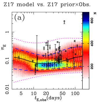
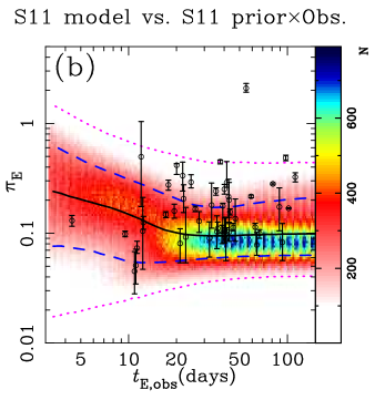
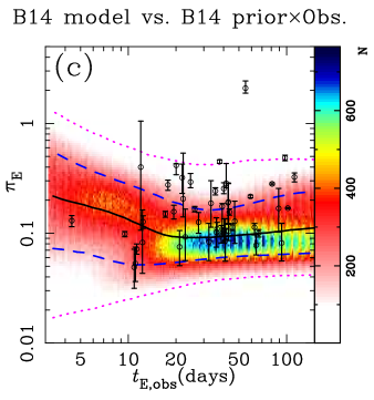
Figure 1: Comparison of the observations with the Galactic model. Each panel shows a different Galactic model. Open circles are the median, $\widetilde{\pi}_{\rm E,post}$, and 68% confidence intervals of the posterior distribution $f_{\rm post}(\pi_{\rm E})$ for the 50 measurements from 2015 Spitzer microlensing campaign (the “raw” sample of Zhu et al., 2017) convolved with the prior from each Galactic model. The color maps indicate the event rate, $\Gamma_{\rm Gal}(\pi_{\rm E}\,|\,t_{\rm E,obs})$. $10^{5}$ artificial events are generated for each bin of $t_{\rm E,obs}$ with the width 0.05 dex. The black solid, blue dashed, and magenta dotted lines indicate the median, $1~{}\sigma$, and $2~{}\sigma$ for $\Gamma_{\rm Gal}(\pi_{\rm E}\,|\,t_{\rm E,obs})$, respectively.

4 Microlensing Event Sample

We use the 50 single microlens events discovered by OGLE-IV survey and observed by the 2015 Spitzer campaign (Zhu et al., 2017), as our event sample. This is the raw sample of Zhu et al. (2017). The $\pi_{\rm E}$ distribution of this sample follows $f_{\rm obs}(\pi_{\rm E}\,|\,t_{\rm E,obs},t_{\rm 0,obs},u_{\rm 0,obs},F_{\rm S,obs})$ and satisfies Eq. (7) when the following two assumptions are true:

1. The measured $t_{\rm E}$ and $\pi_{\rm E}$ are both randomly distributed around the true values of those parameters.

2. The event selection process produces no bias in the $\pi_{\rm E}$ distribution of the sample.

Assumption 2 is the reason why we use the Zhu et al. (2017) raw sample instead of their final sample. The Zhu et al. (2017) final sample includes only events where $\pi_{\rm E}$ can be measured, which they define as events with $\sigma(D_{8.3})\leq 1.4~{}$kpc, where $D_{8.3}={\rm kpc}/(\pi_{\rm rel}/{\rm mas}+1/8.3)$. This selection clearly violates assumption 2, since events with small $\pi_{\rm E}$ are much more likely to have large $\sigma(D_{8.3})$ values. In contrast, their raw sample was selected independently of the measured $\pi_{\rm E}$ values, so this selection should not introduce bias into the $\pi_{\rm E}$ distribution of the raw sample. Note that the Spitzer target selection procedure (Yee et al., 2015a) does favor bright sources, which could violate assumption 2. We show that this does not affect our conclusions in Section 6.2.

4.1 Applying the Galactic Prior to Parallax Measurements

Microlensing parallax measurements typically have large uncertainties because the effect is difficult to measure. Microlensing parallax measurements by satellites, like Spitzer, typically have multiple degenerate solution (Refsdal, 1966; Gould, 1994), and microlensing parallax signals due to the orbital motion of the Earth generally have very large uncertainties in the direction perpendicular to the acceleration of Earth at the time of the event (e.g., Muraki et al., 2011; Bhattacharya et al., 2018). Even when assumption 1 is true, these large uncertainties mean that the assumed prior distribution can have an important influence on the inferred ${\mbox{\boldmath$\bf\pi$}_{\rm E}}$ distribution. In particular, if no prior is applied, it is equivalent to applying a uniform prior, and this can lead to overestimates of $\pi_{\rm E}$ in situations where the true $\pi_{\rm E}$ values are near the limits of the measurement method. Zhu et al. (2017) apply the Galactic prior to derive the distributions of the lens mass and distance, but the reported ${\mbox{\boldmath$\bf\pi$}_{\rm E}}$ values are the one with the uniform prior.

We apply the Galactic prior to generate the following posterior distribution for each event

$$f_{\rm post}(\pi_{\rm E,N},\pi_{\rm E,E})\propto\sum_{i}\Gamma_{\rm Gal}(\pi_{\rm E,N},\pi_{\rm E,E}\,|\,t_{{\rm E,obs},i})$$

$$\times{\cal N}(\pi_{\rm E,N};\pi_{{\rm E,N,obs},i},\sigma^{2}_{\pi_{\rm E,N},i}) {\cal N}(\pi_{\rm E,E};\pi_{{\rm E,E,obs},i},\sigma^{2}_{\pi_{\rm E,E},i})e^{-\Delta\chi^{2}_{i}/2},$$ (13)

where the summation is conducted over the degenerate solutions for each event. ${\cal N}(x;\,{\overline{x}},\sigma^{2}_{x})$ is the Gaussian distribution with the mean of ${\overline{x}}$ and the standard deviation of the measurement error $\sigma_{x}$, where we use the best-fit values and error-bars for $\pi_{\rm E,N}$ and $\pi_{\rm E,E}$ reported by Zhu et al. (2017) as the mean and error, respectively. The Einstein radius crossing times for each of the degenerate solutions, $t_{{\rm E,obs},i}$, are nearly identical, so we calculate the posterior distribution with one representative $t_{\rm E,obs}$ value for each event. Note that Zhu et al. (2017) apply both the Galactic prior and the “Rich” argument (Calchi Novati et al., 2015a), which gives a prior of $\pi_{\rm E}^{-2}$, to their derivation of the distribution of lens masses and distances. This is incorrect as the “Rich” argument is just a crude attempt to apply a prior to the $\pi_{\rm E}$ measurement and it is already included in the Galactic prior. A more recent paper Gould (2020), inspired by an early version of this paper, confirms our identification of the “Rich” argument as a Galactic prior.

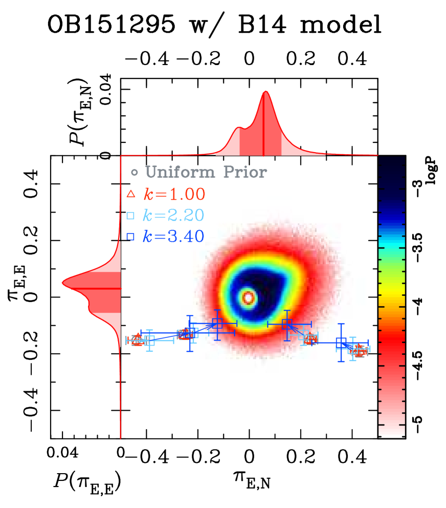
Figure 2: The color coding indicates the two dimensional microlensing parallax prior distribution for event OGLE-2015-BLG-1295 according to the B14 model. The prominent extension in the NNE direction where the probability is highest is the direction of Galactic disk rotation. This is the preferred microlensing parallax direction for lens stars in the Galactic disk. The red boxes with error bars are the median and 68% confidence interval for the posterior distributions for the 4 degenerate Spitzer microlensing parallax measurements for this event. The cyan and blue boxes with error bars indicate the median and 68% confidence intervals for the posterior distribution for the Spitzer microlensing parallax values when the error bars are inflated by factors of $k=2.2$ and 3.4, respectively. The measured values seem consistent with the prior only for the largest error bar inflation factor of $k=3.4$.

An example of how the application of this prior changes the inferred posterior distribution is shown in Figure 2. This figure shows the ${\mbox{\boldmath$\bf\pi$}_{\rm E}}$ prior distribution for event OGLE-2015-BLG-1295, an event with $t_{\rm E}\simeq 42\,$days, and this figure indicates that microlensing parallax values in the range of $0.05\lower 2.15277pt\hbox{$\;\buildrel<\over{\sim}\;$}\pi_{\rm E}\lower 2.15277pt\hbox{$\;\buildrel<\over{\sim}\;$}0.2$ are favored. There is also a strong enhancement of the prior probability in the NNE direction, particularly at larger $\pi_{\rm E}$ values. This is the direction of Galactic disk rotation, which is preferred because of the large number microlensing events due to bulge source stars and lens stars orbiting in the disk. Also, note that values of $\pi_{\rm E}<0.01$ are strongly disfavored, contrary to what the “Rich” argument would imply.

Figure 2 also shows the measured ${\mbox{\boldmath$\bf\pi$}_{\rm E,obs}}$ values as grey circles, as well as the centroid of the posterior probability distribution obtained by convolving this prior with a 2-dimensional Gaussian describing the measurement and its error bars. The medians of the posterior distributions for the 4 degenerate solutions are indicated by red triangles with error bars indicating the 68% confidence interval in both directions. (Note that the red triangles are located in almost exactly the same place as the grey circles for this event.)

We now apply the prior to all 50 of the events in the Zhu et al. (2017) sample, and then, we convert the two dimensional posterior distribution for ${\mbox{\boldmath$\bf\pi$}_{\rm E}}$, $f_{\rm post}(\pi_{\rm E,N},\pi_{\rm E,E})$, into the posterior distribution for the length of the parallax vector, $\pi_{\rm E}$. This posterior distribution is therefore

$$f_{\rm post}(\pi_{\rm E})=\int_{\phi_{\rm E}}f_{\rm post}(\pi_{\rm E},\phi_{\rm E})\,d\phi_{\rm E}$$ (14)

where $\phi_{\rm E}$ is the direction angle of ${\bm{\pi}_{\rm E}}$ vector. and then use for the statistical test. The black open circles in each panel of Figure 1 show the median, $\widetilde{\pi}_{\rm E,post}$, and 68% confidence intervals of $f_{\rm post}(\pi_{\rm E})$ as a function of the observed values of $t_{\rm E,obs}$ for all 50 events in the Z17 sample. For the prior distribution in each of $f_{\rm post}(\pi_{\rm E})$ calculation, we use the compared Galactic model in each panel with parameters for each event (coordinate, Earth projected velocity at $t_{\rm 0,obs}$, etc.). The difference between the different Galactic priors are responsible for the different distributions the black open circles in different panels of Figure 1.

At first glance, only one event is an obvious outlier compared to the model distribution in Figure 1, and most of the other events’ $\widetilde{\pi}_{\rm E,post}$ values are within $\pm 2~{}\sigma$ of the simulated event rate distribution, $\Gamma_{\rm Gal}(\pi_{\rm E}\,|\,t_{\rm E,obs})$. As a result, it would be difficult to argue that the $\pi_{\rm E}$ values measured by Spitzer are too large on an event-by-event basis. However, when we consider all 50 measurements, we see that most events (37 for the S11, B14 models and 40 for the Z17 model) have measurement posteriors, $\widetilde{\pi}_{\rm E,post}$, above the median values (for each individual $t_{\rm E,obs}$ value). The probabilities of these outcomes is given by the binomial distribution, and the probability for at least 37 events above the median is $4.6\times 10^{-4}$, while the probability for $\geq 40$ events above the median is $1.2\times 10^{-5}$. This indicates a strong inconsistency between the $\pi_{\rm E}$ measurements with the Galactic models. It is also obvious that the observations do not match the models by a visual comparison.

4.1.1 Error Bar Inflation Factors

In Section 7, we will conclude that the discrepancy is mainly due to systematic errors in the Spitzer microlensing parallax measurements. As we discuss in Section 7.3, we feel that the optimal way to deal with this problem with the Spitzer microlensing parallax measurements is to try to remove or correct systematic errors in the Spitzer photometry. This is beyond the scope of this work, but it is an approach that has been tried for a few events by Gould et al. (2020) and Dang et al. (2020), inspired, at least in part, but an early version of the work presented here. However, it is not yet clear how successful these approaches will be when applied to a large sample of events. So, we consider a simpler approach, in which we attempt to mitigate the effect of the systematic errors by increasing (or inflating) the error bars of ${\mbox{\boldmath$\bf\pi$}_{\rm E,obs}}$ by a factor $k$, that we refer to as the error bar inflation factor. The idea behind this is to give an estimate of the effect of these systematic errors on the parallax measurement uncertainties and to provide a crude way to correct the measurements in cases where systematic photometry errors cannot be corrected. As we discuss in Section 5, this procedure has some drawbacks when $k$ is very large, but we feel that these error bar inflation factors provide a useful way to characterize the apparent systematic errors.

In Figure 2, the red triangles appear to be strongly inconsistent with the prior distribution for this event, so we also consider the same convolutions of the Galactic prior distributions with Gaussians describing the ${\mbox{\boldmath$\bf\pi$}_{\rm E,obs}}$ measurements with inflated error bars. The cyan and blue boxes with error bars indicate the posterior distributions medians and 68% confidence intervals when the error bars increased by inflation factors of $k=2.2$ and $k=3.4$, respectively. An inflation factor of $k=3.4$ seems to be enough to make two or three of the degenerate solutions consistent with the prior for this event.

We note that the modification of these parallax values to the median of the posterior values will certainly change the predicted Spitzer light curves and they do not follow the original data points. However, this is expected because the introduction of $k>1$ is motivated by the idea that the original Spitzer light curve photometry suffered from systematic errors.

We also apply the error bar inflation factor of 3.4 to the comparison between the Spitzer $\pi_{\rm E}$ measurements and the B14 model from Figure 1(c). The result is shown in Figure 3(a), which indicates that this changes the situation quite dramatically. The obvious discrepancy between models and the Spitzer microlensing parallax measurements largely disappears when the measurement errors are increased by a factor of 3.4.

5 Statistical Tests

We now introduce the inverse percentile, which is defined as $x(y)$ $(0\leq x\leq 1)$ when $y$ is the $100x$-th percentile of a given probability density function of $y$, to more quantitatively evaluate the mismatch between the Spitzer microlensing parallax measurements and the models. The observed value of an observable quantity that follows a given distribution should have a uniform inverse percentile distribution from 0 to 1. Therefore, if the parallax measurement for each event follows the predicted Galactic prior, $\Gamma_{\rm Gal}(\pi_{\rm E}\,|\,t_{\rm E,obs})$, the position of the measured $\pi_{\rm E}$ values with respect to the Galactic prior for each event,

$$P_{\rm Gal}(\pi_{\rm E,prior}\geq\pi_{\rm E}\,|\,t_{\rm E,obs})\equiv\int_{\pi_{\rm E}}^{\infty}\Gamma_{\rm Gal}(\pi_{\rm E}^{\prime}\,|\,t_{\rm E,obs})\,d\pi_{\rm E}^{\prime}\ ,$$ (15)

should follow a uniform distribution as long as a proper Bayesian prior is included in the determination of the measured $\pi_{\rm E}$ value. $P_{\rm Gal}(\pi_{\rm E,prior}\geq\pi_{\rm E}\,|\,t_{\rm E,obs})$ ranges from 0 to 1, depending on the measured $\pi_{\rm E}$ value. A $\pi_{\rm E}$ value that gives $P_{\rm Gal}(\pi_{\rm E,prior}\geq\pi_{\rm E}\,|\,t_{\rm E,obs})=x$ is the $100x$-th percentile of the Galactic prior $\Gamma_{\rm Gal}(\pi_{\rm E}\,|\,t_{\rm E,obs})$, so we refer to $P_{\rm Gal}(\pi_{\rm E,prior}\geq\pi_{\rm E}\,|\,t_{\rm E,obs})$ as the inverse percentile in this paper.

We use the Anderson-Darling (AD) test, which is more sensitive than the commonly used Kolmogorov-Smirnov (KS) test, to compare the inverse percentile distribution from the Spitzer microlensing parallax measurements to the uniform distribution. For each inverse percentile calculation, we use the parameters for each event, which include the event’s Galactic coordinates and the Earth’s velocity at the time of the event peak, $t_{\rm 0,obs}$.

One issue that we face is the choice of the measured value to be used for $\pi_{\rm E}$ in equation (15). Our aim is to compare the posterior distributions, $f_{\rm post}(\pi_{\rm E})$, for the measured values with the Galactic model prior distributions $\Gamma_{\rm Gal}(\pi_{\rm E}\,|\,t_{\rm E,obs})$, and our first choice is to use the median, $\widetilde{\pi}_{\rm E,post}$, to represent the posterior distribution ($f_{\rm post}(\pi_{\rm E})$). This is the same choice that we made for Figure 1, but now we are preparing to invoke this choice in a more elaborate statistical test. This more elaborate test will also involve the error bar inflation factors $k$ that were first discussed in the contest of Figure 2. We also consider $k>1$ because the $f_{\rm post}(\pi_{\rm E})$ distributions with $k=1.0$ appear to be inconsistent with the Galactic model according to our visual inspection on Figure 1 and the binomial tests discussed above. Figure 3(a) shows the effect on $\widetilde{\pi}_{\rm E,post}$ values by applying an error bar inflation factor of 3.4 to the posterior, $f_{\rm post}(\pi_{\rm E})$, distribution for model B14.

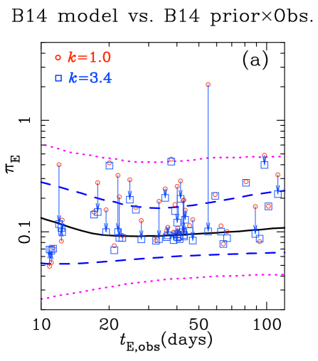
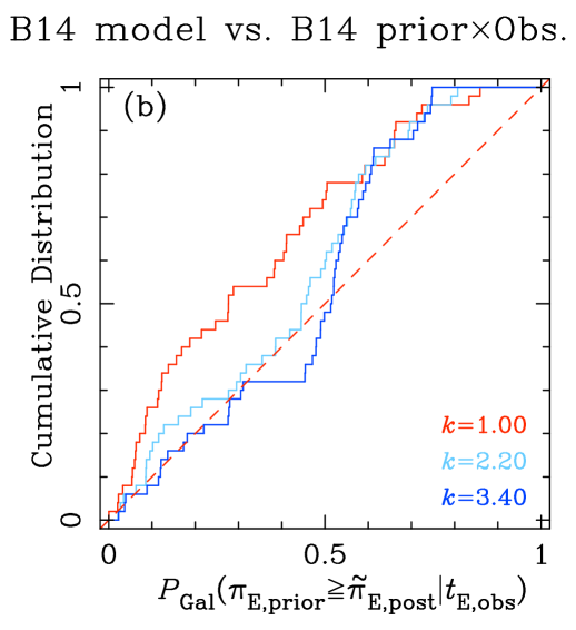
Figure 3: Panel (a) compares of the Spitzer $\pi_{\rm E}$ measurements to the B14 Galactic model, similar to Figure 1(c). The red circles and blue squares indicate the median values, $\widetilde{\pi}_{\rm E,post}$, of the posterior distributions, $f_{\rm post}(\pi_{\rm E})$, with the ${\mbox{\boldmath$\bf\pi$}_{\rm E}}$ error bar inflation factors $k=1.0$ and $k=3.4$, respectively. The red open circles correspond to the black open circles in Figure 1(c). Panel (b) shows the cumulative distribution of the inverse percentiles corresponding to the median $\widetilde{\pi}_{\rm E,post}$, $P_{\rm Gal}(\pi_{\rm E,prior}\geq\widetilde{\pi}_{\rm E,post}\,|\,t_{\rm E,obs})$, with error bar inflation factors of $k=1.0$ (red), $k=2.2$ (cyan), and $k=3.4$ (blue).

Figure 3(b) shows the cumulative distribution of the inverse percentiles calculated for the median, $\widetilde{\pi}_{\rm E,post}$, i.e., the cumulative $P_{\rm Gal}(\pi_{\rm E,prior}\geq\widetilde{\pi}_{\rm E,post}\,|\,t_{\rm E,obs})$ distribution for three different error bar inflation factors, $k=1.0,2.2$, and 3.4. For $k=1.0$, in red, the cumulative distribution is very far from the expected uniform distribution (red dashed line), as expected from the binomial tests discussed above. But for $k=2.2$, the cumulative inverse percentile distribution (cyan) for the $\widetilde{\pi}_{\rm E,post}$ values comes close to the uniform distribution for $P_{\rm Gal}(\pi_{\rm E,prior}\geq\widetilde{\pi}_{\rm E,post}\,|\,t_{\rm E,obs})<0.5$, but it rises up to meet the $k=1.0$ solution for $P_{\rm Gal}(\pi_{\rm E,prior}\geq\widetilde{\pi}_{\rm E,post}\,|\,t_{\rm E,obs})>0.6$. For an error bar inflation value of $k=3.4$, the effect is even more extreme, and we begin to see a collection of events at $P_{\rm Gal}(\pi_{\rm E,prior}\geq\widetilde{\pi}_{\rm E,post}\,|\,t_{\rm E,obs})\approx 0.5$. This is also seen in Figure 3(a) where there is a collection of events near the median (black solid line). This is not surprising. In the limit where $k\rightarrow\infty$, the $f_{\rm post}(\pi_{\rm E})$ values will approach the prior values, since a measurement with infinite error bars is equivalent to no measurement at all. Thus, the $\widetilde{\pi}_{\rm E,post}$ values will approach the medians of the prior distribution and the cumulative distribution will approach a step function at $P_{\rm Gal}(\pi_{\rm E,prior}\geq\widetilde{\pi}_{\rm E,post}\,|\,t_{\rm E,obs})=0.5$.

Statistically, the application of $k>1.0$ should generate posterior distributions $f_{\rm post}(\pi_{\rm E})$ that are a better match to the models. With no error bar inflation, the Bayesian posterior median values are above the median B14 model ($\pi_{\rm E}=\widetilde{\pi}_{\rm E,B14}$) values for 37 of 50 events, and the probability that $\widetilde{\pi}_{\rm E,post}>\widetilde{\pi}_{\rm E,B14}$ for $\geq 37$ events is $4.6\times 10^{-4}$ if we assume that the binomial distribution is appropriate. For error bar inflation factors of $k=2.2$ and 3.4, we have $\widetilde{\pi}_{\rm E,post}>\widetilde{\pi}_{\rm E,B14}$ for 30 and 24 events, respectively. The binomial distribution would imply probabilities of 0.10 and 0.66 for these two cases of $k=2.2$ and 3.4, respectively. We can also apply the Anderson-Darling test formula to get “probabilities” of $1.7\times 10^{-5}$, $8.4\times 10^{-5}$, and $9.1\times 10^{-3}$ for $k=1.0$, $k=2.2$ and 3.4, respectively.

However, when the error bars are large, the conditions for the AD test do not really apply. The test was designed to compare a theoretical distribution with measurements without regard to error bars. In a situation with large error bars and a steeply varying prior, the posterior distributions of the measurements can be significantly different from the measured values. As a result, we can see a significant shift of the $\widetilde{\pi}_{\rm E,post}$ values toward the median of the prior distribution, as we have see from Figure 3 for $k=3.4$.

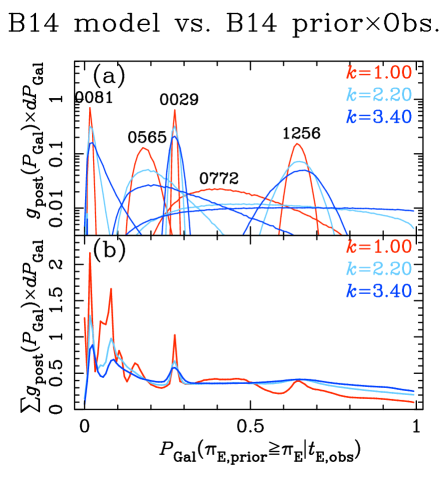
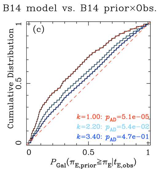
Figure 4: Panel (a) shows the posterior probability distributions of the inverse percentile $P_{\rm Gal}(\pi_{\rm E,prior}\geq\pi_{\rm E}\,|\,t_{\rm E,obs})$, $g_{\rm post}(P_{\rm Gal})$, for 5 events from the Zhu et al. (2017) sample with the B14 Galactic prior. The y-axis values are probabilities integrated over bins of width $dP_{\rm Gal}=0.008$. The red, cyan, and blue curves show the probability distributions as the error bar inflation factors change from $k=1.0$ (red), to $k=2.2$ (cyan), and finally to $k=3.4$ (blue). Panel (b) shows the sum of these distributions over all 50 events of the Zhu et al. (2017) sample, $\sum g_{\rm post}(P_{\rm Gal})$, with the same color scheme for the error bar inflation factors. The cumulative density functions (CDFs) of the inverse percentile, $G_{\rm post}(P_{\rm Gal})$, are shown in the panel (c). The over-plotted black discrete cumulative distributions are created by dividing the vertical axis into 50 (i.e., number of events) bins, and these are used for our statistical tests. The results of AD tests are shown in the bottom right of panel (c).

The simplest way to modify the cumulative distributions in Figure 3(b) to allow proper AD tests would be to randomly sample $\pi_{\rm E}$ from the posterior distribution $f_{\rm post}(\pi_{\rm E})$ for each event to obtain a sample of randomly selected “measurements” that can be used to create inverse percentile distributions that can be used for the AD tests. We have tried this, but the results are somewhat noisy due to the limited number of events. An alternative, but less noisy approach is to convert $f_{\rm post}(\pi_{\rm E})$ into the posterior distribution of the inverse percentile $P_{\rm Gal}(\pi_{\rm E,prior}\geq\pi_{\rm E}\,|\,t_{\rm E,obs})$, which we refer to as $g_{\rm post}(P_{\rm Gal}(\pi_{\rm E,prior}\geq\pi_{\rm E}\,|\,t_{\rm E,obs}))$. The relation between the two posterior distributions is

$$g_{\rm post}(P_{\rm Gal}(\pi_{\rm E,prior}\geq\pi_{\rm E}\,|\,t_{\rm E,obs}))\,dP_{\rm Gal}=f_{\rm post}(\pi_{\rm E})\,d\pi_{\rm E}\,,$$ (16)

where $dP_{\rm Gal}$ is the differential of the variable $P_{\rm Gal}(\pi_{\rm E,prior}\geq\pi_{\rm E}\,|\,t_{\rm E,obs})$. The posterior inverse percentile distribution $g_{\rm post}(P_{\rm Gal}(\pi_{\rm E,prior}\geq\pi_{\rm E}\,|\,t_{\rm E,obs}))$ is easily calculated by converting each $\pi_{\rm E}$ which follows the posterior distribution $f_{\rm post}(\pi_{\rm E})$ into the inverse percentile, $P_{\rm Gal}(\pi_{\rm E,prior}\geq\pi_{\rm E}\,|\,t_{\rm E,obs})$, using Equation (15). Hereafter, we use the shorter notation $g_{\rm post}(P_{\rm Gal})$ in place of $g_{\rm post}(P_{\rm Gal}(\pi_{\rm E,prior}\geq\pi_{\rm E}\,|\,t_{\rm E,obs}))$. After $g_{\rm post}(P_{\rm Gal})$ is calculated for every event, we sum these distributions for all 50 events and we refer to this combined distribution as $\sum g_{{\rm post}}(P_{\rm Gal})$, or $\sum_{i=1}^{N_{\rm eve}}g_{{\rm post},i}(P_{\rm Gal})$ when we want to explicitly indicate the region for the summation. $(N_{\rm eve}=50$ in this case.) Then, we calculate the cumulative density function (CDF) of the inverse percentile

$$G_{\rm post}(P_{\rm Gal})\equiv\int_{0}^{P_{\rm Gal}}\sum_{i=1}^{N_{\rm eve}}g_{{\rm post},i}(P_{\rm Gal}^{\prime})/N_{\rm eve}\,dP_{\rm Gal}^{\prime},$$ (17)

and divide the vertical axis into $N_{\rm eve}$ (=50) bins to make a discrete cumulative distribution which is used in the AD tests. This is demonstrated in Figure 4(a), which shows individual $g_{\rm post}(P_{\rm Gal})$ for five events with the error bar inflation factors of $k=1.0,2.2,$ and 3.4 as red, cyan, and blue curves respectively. Figure 4(b) shows the sum of $g_{\rm post}(P_{\rm Gal})$ for all 50 events, $\sum g_{\rm post}(P_{\rm Gal})$, with the same color scheme as Figure 4(a). Peaks due to events 0029, 0081, and 1256 are visible in this $\sum g_{\rm post}(P_{\rm Gal})$ distribution without error bar inflation, but the event 1256 peak is washed out with an inflation factor of $k=3.4$, while the peaks corresponding to the other events are diminished. Figure 4(c) shows the CDF of the inverse percentile, $G_{\rm post}(P_{\rm Gal})$, using the three error bar inflation factors $k=1.0,2.2,$ and 3.4 in red, cyan and blue. The AD tests give probabilities of $p_{\rm AD}=5.1\times 10^{-5},0.054$, and 0.47. This confirms that the posterior distribution with $k=3.4$ is consistent with the Galactic model, while the posterior distribution with $k=2.2$ is only marginally consistent with the Galactic model, while the results with the reported error bars are inconsistent with the Galactic model.

We repeat these calculations with all three Galactic models to determine the probabilities with $k=1$ in addition to the minimum value of $k$ needed to be marginally consistent ($p_{\rm AD}=0.05$) and fully consistent ($p_{\rm AD}=0.50$) with each of the Z17, S11, and B14 Galactic models, as indicated in Table 2 and Figure 5. Table 2 shows that the posterior distribution with any Galactic prior fails to match the model predictions with AD probabilities ranging from $4.0\times 10^{-5}$ to $6.6\times 10^{-5}$ when $k=1$. Thus, there is a strong and obvious contradiction between the Spitzer microlensing parallax results and our Galactic models. It is notable that one of our Galactic models is the Z17 model presented by the Spitzer microlensing team (Zhu et al., 2017), but the Z17 model does not fit the distribution of Spitzer microlensing parallax results significantly better than the other two models. We find that $k>2.2$ is minimum error bar correction needed for each of the north and east components of the reported ${\mbox{\boldmath$\bf\pi$}_{\rm E,obs}}$ measurements to make the Spitzer $\pi_{\rm E}$ measurements consistent with the Galactic models, but an error bar inflation factor of $k=3.4$ or 3.5 is needed to match the median prediction of the Galactic models.

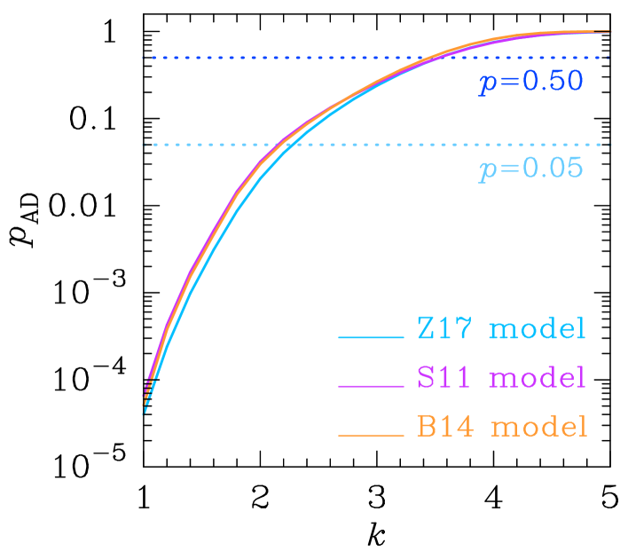
Figure 5: The $p$-values of AD tests for the CDF $G_{\rm post}(P_{\rm Gal})$ as a function of the error bar inflation factor, $k$ for each of our three models, Z17, S11, and B14.

Table 2: Results of AD tests to compare the posterior distributions for the 50 events in the Z17 raw sample and the Galactic model.

Model	$A^{2}$ ($p_{\rm AD}$) w/ $k=1$	$k\,(p_{\rm AD}=0.05)$	$k\,(p_{\rm AD}=0.50)$	$n_{\rm D/B,th}$
Z17	9.01 ($4.0\times 10^{-5}$)	2.27	3.53	3.1
S11	8.54 ($6.6\times 10^{-5}$)	2.14	3.53	3.9
B14	8.78 ($5.1\times 10^{-5}$)	2.17	3.45	4.0

Note. — Indicated model is used both for the Bayesian prior convolved with the Z17 measurements and for the compared model.

We have confirmed our method of using $G_{\rm post}(P_{\rm Gal})$ for AD tests by conducting simple AD tests using $\pi_{\rm E}$ values randomly sampled from $f_{\rm post}(\pi_{\rm E})$ for each event. From 600 trials using the B14 model, we find median values of $p_{\rm AD}=5.2\times 10^{-5}$, $0.042$ and 0.30, for $k=1.0,2.2$ and 3.4, respectively. These are very close to the $p_{\rm AD}$ values of $5.1\times 10^{-5},0.054$, and 0.47 that we found using $G_{\rm post}(P_{\rm Gal})$. The $1~{}\sigma$ ranges of these $p_{\rm AD}$ values are noisy, as expected. They are $5.8\times 10^{-6}$ - $3.0\times 10^{-4}$, $6.9\times 10^{-3}$ - $0.17$ and $0.069$ - $0.70$, respectively.

One might think that the AD test is not designed to be part of a Bayesian analysis. We use the posterior distributions in this paper, though, because we want to be conservative by adding the Galactic prior. We find $p_{\rm AD}$ values of $9.1\times 10^{-9}$, $3.0\times 10^{-8}$ and $6.1\times 10^{-9}$ with the Z17, S11 and B14 model, respectively, when we conduct the AD tests using the original reported $\pi_{\rm E}$ values by Zhu et al. (2017). In the tests, we use a solution that has minimum $\chi^{2}+4\ln\pi_{\rm E}$ value for each event. These values are smaller than the probabilities with the posterior distribution in Table 2 by 3-4 orders of magnitude and this confirms that we are conservative.

6 What Is the Cause of the Discrepancy?

The most obvious potential cause of this discrepancy between the three Galactic models we consider and the Spitzer microlensing parallax values is systematic errors in the Spitzer photometry. This is why we considered the error bar inflation factor $k>1$ in Section 5. Section 5.1 of Zhu et al. (2017) is devoted to a discussion of systematic errors in the Spitzer photometry, and they mention five events with “prominent” deviations of the Spitzer photometry from the best fit light curve. Our visual inspection of the 50 light curves presented in Zhu et al. (2017) indicates that 18 (or 36%) of these have obvious systematic differences between the Spitzer photometry and the best fit microlensing models. Since the microlensing parallax parameters are often determined almost solely from the Spitzer data, it seems quite plausible that some of the events without obvious systematic photometry errors may, nevertheless, have large errors that can be accounted for with incorrect ${\mbox{\boldmath$\bf\pi$}_{\rm E,obs}}$ model parameters. Zhu et al. (2017) suggest that these systematic errors might not cause problems with the Spitzer ${\mbox{\boldmath$\bf\pi$}_{\rm E,obs}}$ measurements with a reference to three events (Udalski et al., 2015; Poleski et al., 2016; Han et al., 2017) for which there is some evidence suggest that the systematic errors may not have much influence on the ${\mbox{\boldmath$\bf\pi$}_{\rm E,obs}}$. But, two of these events have much stronger microlensing signals in the Spitzer data than is typical, so this argument may not apply to the bulk of the Zhu et al. (2017) sample.

Although these obvious systematic photometry problems are an important issue, we also need to consider several other issues that could contribute to this discrepancy. We start by considering the possibility that a plausible Galactic model could be consistent with the data. Then we consider possibility of bias in the Spitzer sample could influence the large $\pi_{\rm E}$ values. We set the error bar inflation factor $k=1$ in all of our subsequent analysis.

6.1 Is There a Galactic Model That Can Match the Spitzer Data?

In this section, we consider modifications to our Galactic models to match the distribution of ${\mbox{\boldmath$\bf\pi$}_{\rm E,obs}}$ values from the Zhu et al. (2017) Spitzer sample. For fixed $t_{\rm E}$ values, microlensing parallax values can be increased by decreasing the lens distance, $D_{L}$, the lens mass, $M_{L}$, and/or the lens-source relative transverse velocities. However, the requirement of fixed $t_{\rm E}$ values, means that the distributions of $D_{L}$, $M_{L}$, and transverse velocity are correlated, and in this section, we consider modifications of the $M_{L}$ and $D_{L}$ distributions of the Galactic models. One parameter that is not very well known is the slope of the initial mass function (IMF) in the brown dwarf mass region, $\alpha_{\rm bd}$. This has been measured in previous microlensing studies (Sumi et al., 2011; Mróz et al., 2017), but these measurements depend on Galactic models similar to (or identical to) the models that we have considered. So, it is sensible to consider variations in the $\alpha_{\rm bd}$ values.

The other parameter that we consider modifications to is the ratio of the disk mass to bulge mass. We define the change relative to the fiducial model disk/bulge mass ratio as

$$n_{\rm D/B}\equiv\frac{(\rho_{\rm D,0}/\rho_{\rm B,0})_{\rm art}}{(\rho_{\rm D,0}/\rho_{\rm B,0})_{\rm org}},$$ (18)

where $(\rho_{\rm D,0}/\rho_{\rm B,0})_{\rm art}$ is the value in an “artificial” model with an increased disk mass and/or a decreased bulge mass, and $(\rho_{\rm D,0}/\rho_{\rm B,0})_{\rm org}$ is the value in the unmodified models presented in Table 1.

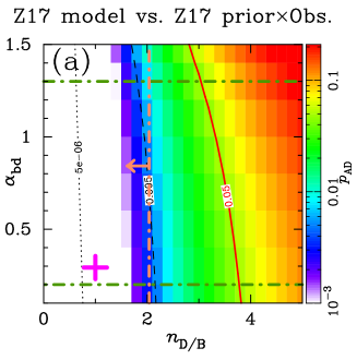
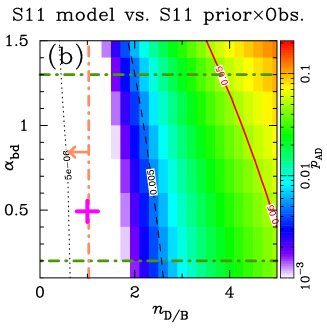
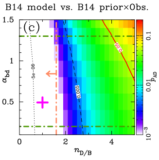
Figure 6: Results of AD tests with various $(n_{\rm D/B},\alpha_{\rm bd})$ combinations, where the modified Galactic model is applied both to the Bayesian prior and to the compared model. Both color maps and contours show $p_{\rm AD}$-values from the AD tests. In each panel, the two horizontal dark green dashed-dotted lines indicate the $3\sigma$ range for $\alpha_{\rm bd}$ from Mróz et al. (2017), the vertical orange dashed-dotted line indicates the $3\sigma$ upper limit on $n_{\rm D/B}$ described in Section 6.1, and the magenta cross indicates the values of $\alpha_{\rm bd}$ and $n_{\rm D/B}$ employed by each of the three models: Z17, S11, and B14.

We compare the CDFs of the inverse percentile, $G_{\rm post}(P_{\rm Gal})$, to the expected uniform distribution, similar to the comparisons presented in Figure 4, for modified versions of the Z17, S11, and B14 on a grid of $n_{\rm D/B}$ and $\alpha_{\rm bd}$ values. We perform the AD test on each such model, and present the resulting probabilities, $p_{\rm AD}$, as a function of $n_{\rm D/B}$ and $\alpha_{\rm bd}$ in Figure 6, where the modified model is also used for the Bayesian prior to calculate $f_{\rm post}(\pi_{\rm E})$ as well as the compared model at each grid. Both the color map and the contours indicate the $p_{\rm AD}$ distribution, and the red contour lines indicate our threshold $p$-value of $p_{\rm AD}\geq 0.05$, which is marginally acceptable.

The brown dwarf mass function slope, $\alpha_{\rm bd}$, has been measured using data from the MOA-II (Sumi et al., 2011), OGLE-III (Wegg et al., 2017), and the OGLE-IV (Mróz et al., 2017) microlensing surveys, with results that are very consistent with each other. OGLE-IV is the most sensitive survey, so we show their 3$\sigma$ limits, $0.2<\alpha_{\rm bd}<1.3$, as the green horizontal dot-dashed lines in Figure 6. If we restrict $\alpha_{\rm bd}$ to lie within this range, then we can use the distributions presented in Figure 6, to derive the minimum values of $n_{\rm D/B}$ required to pass our acceptability threshold of $p_{\rm AD}\geq 0.05$. These results are given in Table 2. The fiducial model values of $n_{\rm D/B}=1$ for each of the Z17, S11, and B14 models are thought to explain the observed $t_{\rm E}$ distributions very well, so if we are required to select $n_{\rm D/B}\gg 1$ in order to get plausible $p_{\rm AD}$ values, this could be taken as an indication that the Spitzer results cannot be explained by any reasonable Galactic model. The results listed in Table 2 are 3.1, 3.9 and 4.0 for the Z17, S11, and B14 models, respectively.

It seems implausible that the disk-to-bulge mass ratio for the Z17, S11, and B14 models could really be increased by a factor of 3.1 or more from the model values and still be consistent with observations, but let us consider this question in more detail. The relative disk-to-bulge mass ratio, $n_{\rm D/B}$, as defined in Eq. (18) will increase when $\rho_{\rm D,0}$ increases, $\rho_{\rm B,0}$ decreases, or both.

From Gaia DR1 (Gaia Collaboration et al., 2016), Bovy (2017) derives a local stellar density of $0.040\pm 0.002~{}M_{\odot}\,{\rm pc}^{-3}$ for main sequence stars. To get the total density, we must add the density of white dwarfs, $0.0065~{}M_{\odot}\,{\rm pc}^{-3}$ (Bovy, 2017), and brown dwarfs, which account for 4.4% as much mass as the main sequence stars (McKee et al., 2015). This gives a total density of $0.048\pm 0.002~{}M_{\odot}\,{\rm pc}^{-3}$. This is $1.26\pm 0.05$ times, $0.81\pm 0.03$ times and $1.24\pm 0.05$ times larger than the $\rho_{\rm D,0}$ values for the Z17, S11, and B14 models. respectively.

Portail et al. (2017) constructed a dynamical model of the bulge, with the aid of N-body simulations, and their model is consistent with the bulge star number counts from the VVV survey (Minniti et al., 2010) and spectroscopic surveys, such as BRAVA (Kunder et al., 2012). Their model was also confirmed to be consistent with the OGLE-II proper motion data (Sumi et al., 2004), microlensing optical depth (Sumi & Penny, 2016), and the $t_{\rm E}$ distribution of OGLE-III (Wyrzykowski et al., 2015; Wegg et al., 2017). They derive stellar mass traced by red clump giants observed by the near infrared surveys in a box of $(\pm 2.2\times\pm 1.4\times\pm 1.2)$ kpc around the principal axes of the bulge to be $(1.32\pm 0.08)\times 10^{10}~{}M_{\odot}$. We integrate the bar models of Z17, S11 and B14 within the box and obtain $1.76\times 10^{10}~{}M_{\odot}$ for the Z17 model and $1.39\times 10^{10}~{}M_{\odot}$ for both the S11 and B14 models. In order to be consistent with the Portail et al. (2017) bulge mass, the normalization of the model bulge masses must be multiplied by $0.75\pm 0.05$ times, $0.95\pm 0.06$ times and $0.95\pm 0.06$ times for the Z17, S11, and B14 models, respectively. Therefore, to be consistent with the recent studies requires $n_{\rm D/B}$ values for Z17, S11, and B14 models to be $1.68\pm 0.12$, $0.85\pm 0.06$, and $1.30\pm 0.10$, respectively. The vertical orange dot-dashed lines in Figure 6 represent the 3$\sigma$ upper limits on $n_{\rm D/B}$ from this calculation, and it is clear that they do not come close to the $p_{\rm AD}\geq 0.05$ contours. In the most favorable case, the Z17 model, the $p_{\rm AD}\geq 0.05$ contour is still excluded by $>10\sigma$ in this most favorable case.

Although we do not consider the change of kinematic property due to the system mass change in the modified models, this effect is not likely to fully help the situation because a large change in $n_{\rm D/B}$ value requires both dynamically hotter disk stars and dynamically cooler bulge stars. These two effects are roughly cancelled in the $\Gamma_{\rm Gal}(\pi_{\rm E}\,|\,t_{\rm E,obs})$ distribution. So we conclude that the reported Spitzer $\pi_{\rm E}$ values are not consistent with any reasonable Galactic model although the level of discrepancy might be mitigated a little by applying a modest change to the Galactic models.

6.2 A Bias in the Spitzer Sample Is Unlikely to Cause the Discrepancy

Another possibility is that the discrepancy between the Galactic models and the Spitzer $\pi_{\rm E}$ values could be due to a bias in the selection of the events in the Z17 sample. One known bias that affects $\pi_{\rm E}$ distribution in the Spitzer sample is that the Spitzer event selection process favors larger $t_{\rm E}$ values. This bias is discussed by Zhu et al. (2017), who also pointed out that the Z17 sample lacks extremely long timescale ($t_{\rm E}\lower 2.15277pt\hbox{$\;\buildrel>\over{\sim}\;$}100$ days). A bias in the $t_{\rm E}$ distribution for the Z17 sample does not affect our analysis because we consider the event rate, $\Gamma_{\rm Gal}(\pi_{\rm E}\,|\,t_{\rm E,obs})$, as a function of $t_{\rm E,obs}$, as discussed in Section 2.

A modest bias that does exist in the Z17 sample concerns the source brightness. According to Yee et al. (2015a), events with brighter sources are favored. The selection of brighter sources provides a bias in favor of smaller source distances, $D_{\rm S}$. The Galactic models consider a source distance dependence for the event rate that is weighted by proportional to $D_{\rm S}^{2-\gamma}$, so we can evaluate the effect of this bias by varying $\gamma$.

However, as described in Section 3.4 and summarized in Table 1, we have already used three models with very different $\gamma$ values, ranging from 1.5 for the B14 model to 2.85 for the Z17 model, but the $p$-values for these models are very similar. This is similar to the analysis of Zhu et al. (2017) who found that variation of the $\gamma$ value had little effect on their results (see Appendix A of their paper). We have also conducted the AD-test for the B14 model with $\gamma=2.85$, instead of the original value of 1.5, and we find $p_{\rm AD}=8.7\times 10^{-5}$. This is a slight improvement over the original $p_{\rm AD}=5.1\times 10^{-5}$ value for this model, so it does account for the discrepancy. Thus, sample bias cannot explain the failure of the Spitzer $\pi_{\rm E,obs}$ sample to match the Galactic models.

7 Spitzer’s Systematic Photometry Errors

In Section 6, we have established that the systematically large $\pi_{\rm E}$ values found by Zhu et al. (2017) are neither likely to be an artifact of inadequate Galactic models nor caused by any selection bias in their sample. Now we consider the idea that this discrepancy is due to systematic errors in the Zhu et al. (2017) $\pi_{\rm E}$ measurements, which seems to be the only reasonable conclusion. The $t_{\rm E,obs}$ measurements by OGLE have been shown to be very accurate and unbiased (Mróz et al., 2017), but it is possible that systematic errors in the OGLE photometry could contribute to the systematic errors in the $\pi_{\rm E}$ measurements for some of the longer duration events. However, the main purpose of the Spitzer survey is to measure $\pi_{\rm E}$, and the Spitzer measurements are known to dominate the $\pi_{\rm E}$ for some long duration events (Poleski et al., 2016).

In this section, we first report our findings that the level of discrepancy is correlated with three different aspects in the events in the Z17 sample. These are the source magnitude $I_{\rm S}$, the light curve peak coverage by Spitzer, and whether or not an obvious systematic error is seen in the Spitzer light curves shown in Figure 4 of Zhu et al. (2017). This is not only useful to understand how the systematic errors affect the parallax measurements, but also another conclusive evidence that the discrepancy we have discussed mainly attributes to the Spitzer light curves rather than the Galactic models or our method. Then we discuss possible ways to account for the systematic errors including some recent attempts by other authors. Finally we compare our study with Shan et al. (2019) and Zang et al. (2020) who conducted statistical tests on much smaller samples of Spitzer events that might plausibly be reinterpreted as tests of consistency of their samples with Galactic models.

7.1 Correlation Between Systematic Errors and Event Characteristics

One way to help us find nature of the systematic errors is to consider possible correlations between the apparent systematic errors and the characteristics of the events in the sample. To address this question, we conduct the statistical tests on a number of Z17 sub-samples based on several different event characteristics. This investigation has revealed that the $p$-values depend on the source star brightness, the coverage of the light curve peak in the Spitzer data, and the presence of obvious systematic discrepancies between the Spitzer data and the best fit light curve models. These correlations help to elucidate the nature of the systematic errors in the Spitzer data. For the remainder of this paper, we will use the B14 model with the error bar inflation factor $k=1$ for our tests, unless we specifically indicate that we are using another model. Results from other models are provided in some of the tables, and our conclusions do not depend on which Galactic model is used.

7.1.1 Correlation with the Source Brightness

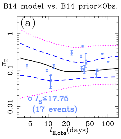
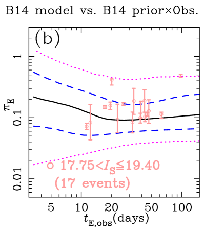
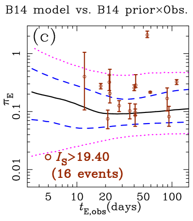
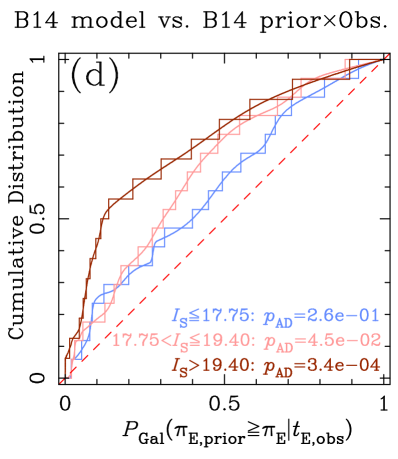
Figure 7: Panels (a)-(c) are similar to Fig. 1 (c), but only plot events which have the source magnitude $I_{\rm S}$ in the indicated range in each panel. Panel (d) is the CDFs of the inverse percentile, $G_{\rm post}(P_{\rm Gal})$, for each sample shown in the panels (a)-(c).

In general, observations of bright stars provide a high signal-to-noise ratio and they are likely to be less affected by systematic errors, except those, like flat-fielding errors that are proportional to the star’s brightness. Motivated by this thought, we divide all 50 events of the Zhu et al. (2017) raw sample into three groups based on the source magnitude reported by Zhu et al. (2017). The three groups consist of 17, 17 and 16 events which have the source $I$-band magnitude $I_{\rm S}\leq 17.75$, $17.75<I_{\rm S}\leq 19.40$ and $I_{\rm S}>19.40$, respectively. These boundaries of $I_{\rm S}$ are seleccted to make the number of events in each group nearly equal so that results of the AD tests below are not dominated by the different sample sizes. The sensitivity of these subsamples of 16 or 17 events is reduced compared to the full sample of 50 events. To evaluate this effect, we have conducted Monte Carlo simulations of $10^{4}$ AD tests each with randomly selected 16 and 17 event sub-samples of the full Z17 sample. These yield median $p_{\rm AD}$ values of $p_{\rm AD}=0.026$ and $p_{\rm AD}=0.022$ for the 16 and 17 event subsamples, respectively, which compare to $p_{\rm AD}=5.1\times 10^{-5}$ for the full 50 event sample. Note that, although the source flux in IRAC 3.6 $\mu$m may seem to more directly represent the brightness of events seen by Spitzer, we do not choose it here because the source flux is one of the model parameters and measurements of the source flux in IRAC 3.6 $\mu$m could be contaminated by the systematic errors in Spitzer data. On the other hand, the source flux in $I$-band is well measured by OGLE data and is unlikely to be affected by the systematic errors.

Figure 7 shows plots similar to Figures 1(c) and 4(c), but for each of the three source brightness sub-samples with no error bar inflation (i.e., $k=1.0$). In panels (a)-(c), the five curves are the median, $1\sigma$ and $2\sigma$ curves from the B14 model. Panel (a) shows that the brightest stars still tend to have $\widetilde{\pi}_{\rm E,post}$ values larger than the model predictions, but the distribution of $\pi_{\rm E}$ values for the $17.75<I_{\rm S}\leq 19.40$ subsample (b) and especially the faint event subsample (c) are much more strongly skewed toward larger $\pi_{\rm E,obs}$ values. This is quantitatively confirmed by the $p$-values from AD-tests for the CDFs of the inverse percentile plotted in panel (d), where $p_{\rm AD}=0.26$, $0.045$ and $3.4\times 10^{-4}$ are obtained for the bright, middle and faintest subsamples, respectively. This result indicates that there is a correlation between $p_{\rm AD}$ values and the source brightness of events used in the test. Table 3 shows the results of these AD tests with all three Galactic models.

Table 3: Results of AD tests on events in three different source brightness ranges.

Model	$A^{2}$ ($p_{\rm AD}$) w/ $k=1$			$k\,(p_{\rm AD}=0.05)$ for
	$I_{\rm S}\leq 17.75$	$17.75<I_{\rm S}\leq 19.40$	$I_{\rm S}>19.40$	$I_{\rm S}>17.75$ events
	(17 events)	(17 events)	(16 events)
Z17	1.7 ($0.13$)	3.1 ($0.026$)	5.7 ($1.4\times 10^{-3}$)	2.77
S11	1.2 ($0.27$)	2.4 ($0.054$)	7.0 ($3.7\times 10^{-4}$)	2.61
B14	1.2 ($0.26$)	2.6 ($0.045$)	7.0 ($3.4\times 10^{-4}$)	2.61

This result is consistent with the idea that the systematic errors have a larger effect on the parallax measurement for fainter sources. In particular, the effects of the systematic errors on the parallax measurements are much smaller for the 17 events with $I_{\rm S}\leq 17.75$ than for the other sub-samples with fainter source stars. The AD tests on this bright source star sub-sample give $p_{\rm AD}=0.13$, 0.27 and 0.26 for the Z17, S11 and B14 models, respectively. Thus, they are formally consistent with all the three Galactic models used in this paper if we apply the acceptable $p$-value range of $p_{\rm AD}\geq 0.05$ that is used in Section 6.1, although part of the improvement compared to the full sample of 50 events is due to the statistical noise for a smaller sample size. Note that the selection bias due to the preference to include brighter source star in the Spitzer sample inserts very little bias into the measured $\pi_{\rm E}$ distribution, as discussed in Section 6.2.

7.1.2 Correlation with Light Curve Peak Coverage by Spitzer

The role of observed data points for light curve modeling is highly dependent on what part of the light curve they cover. To measure the microlensing parallax using Spitzer for a single lens event, the most important part is the light curve magnification peak because ${\mbox{\boldmath$\bf\pi$}_{\rm E}}$ is given by

$${\mbox{\boldmath$\bf\pi$}_{\rm E}}\simeq\frac{\rm AU}{D_{\perp}}\left(\frac{\Delta t_{0}}{t_{\rm E}},\Delta u_{0}\right)\ ,$$ (19)

where $D_{\perp}$ is the separation between the Earth and Spitzer perpendicular to the event direction and $\Delta t_{0}$ and $\Delta u_{0}$ are differences of the time at the event peak, $t_{0},$ and impact parameter, $u_{0}$, seen by the Earth from those seen by Spitzer. Because ${\mbox{\boldmath$\bf\pi$}_{\rm E}}\parallel{\mbox{\boldmath$\bf\mu$}_{\rm rel}}$, $\Delta t_{0}\propto$ the component of ${\mbox{\boldmath$\bf\pi$}_{\rm E}}$ in the direction of the Earth-satellite separation and $\Delta u_{0}\propto$ the perpendicular component of ${\mbox{\boldmath$\bf\pi$}_{\rm E}}$. For the location of the Galactic bulge microlensing fields at RA $\sim 18$h and DEC $\sim-30^{\circ}$, Spitzer is largely to the West of Earth at the time of the Spitzer observations. Thus, $\Delta t_{0}$ largely determines $\pi_{\rm E,E}$ and $\Delta u_{0}$ largely determines $\pi_{\rm E,N}$. Because $t_{0}$ is time of peak magnification and $u_{0}$ is the impact parameter that determines the peak magnification, observations over the peak in a single lens light curve are crucial to definitively determine the microlens parallax. We also note that, in general, observations only near the light curve peak are not sufficient to determine $u_{0}$, and consequently $\pi_{\rm E,N}$.

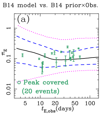
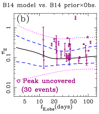
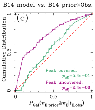
Figure 8: Same as Figure 7, but for the peak covered events and the peak uncovered events.

The majority of the Spitzer events do not have the Spitzer observations over their peak. Instead, they have data only for rising or declining part of the symmetric single lens light curve. Visual inspection of the Z17 Spitzer data indicate that the $t_{0}$ value for the Spitzer can be easily determined for only 20 of the 50 Z17 events. These are events: 0379, 0565, 0798, 0843, 0958, 0961, 0965, 1161, 1172, 1188, 1189, 1256, 1341, 1370, 1420, 1448, 1450, 1457, 1482 and 1533, where the numbers correspond to the event “OGLE-2015-BLG-????”. Hereafter, we refer to these 20 events as the peak covered events and the other 30 events as the peak uncovered events. Figures 8 (a)-(b) show the distributions of $t_{\rm E,obs}$ and $\widetilde{\pi}_{\rm E,post}$ for these two samples and Figure 8 (c) shows results of AD tests on these samples using the B14 model. These two samples have clearly different distributions from each other. For the peak covered sample, we find the probability of $p_{\rm AD}=0.54$ which is even larger than our fully acceptable threshold probability of $p_{\rm AD}=0.50$ that is used in Section 5. However, part of this improvement is due to the smaller sample size. Monte Carlo simulations of $10^{4}$ AD tests for a randomly selected 20 event sub-sample of the Z17 sample give $p_{\rm AD}=0.013$, which compares to $p_{\rm AD}=5.1\times 10^{-5}$ for the full 50 event sample. For the peak uncovered sample, we find $p_{\rm AD}=2.4\times 10^{-6}$. This compares to $p_{\rm AD}=2.0\times 10^{-3}$ for a random sub-sample of 30 events and $p_{\rm AD}=5.1\times 10^{-5}$ for the full sample. Obviously, the lack of Spitzer light curve peak coverage leads to larger systematic errors. Results with the S11 and Z17 models are shown in Table 4, which confirm the same trend.

Table 4: Results of AD tests on events with and without peak coverage by Spitzer.

Model	$A^{2}$ ($p_{\rm AD}$) w/ $k=1$		$k\,(p_{\rm AD}=0.05)$ for
	Peak covered	Peak uncovered	peak uncovered events
	(20 events)	(30 events)
Z17	2.0 ($0.098$)	9.4 ($2.6\times 10^{-5}$)	2.94
S11	0.6 ($0.63$)	11.6 ($2.7\times 10^{-6}$)	2.56
B14	0.7 ($0.54$)	11.7 ($2.4\times 10^{-6}$)	2.61

One issue in these two samples contain is a possible bias created due to the selection based on whether the Spitzer covered the event peak or not. Because the Spitzer observations start always 3 to 9 days after the event selection, it is somewhat easier for Spitzer to cover the event peak when it comes later than the peak seen by the Earth. However, the Spitzer event selection procedure helps to mitigate this effect (Yee et al., 2015a) by preferentially selecting events that are alerted well before the peak. This causes a slight bias in the $\pi_{\rm E,E}$ distribution between these two samples because $\pi_{\rm E,E}$ is mostly determined by $\Delta t_{0}/t_{\rm E}$ in Equation (19), and this favors $\pi_{\rm E,E}<0$ in the peak covered sample. However, the peak uncovered sample also has a similar bias. Events with Spitzer observations only after the peak may have no real ${\mbox{\boldmath$\bf\pi$}_{\rm E}}$ signal in the Spitzer. If so, possible systematic errors would lead to an apparent $\pi_{\rm E,E}$ value less than the true value. So, the $\pi_{\rm E}$ distribution could be biased because $\pi_{\rm E}=\sqrt{\pi_{\rm E,E}^{2}+\pi_{\rm E,N}^{2}}$, but it is unclear if this bias would affect our tests. We expect that whatever bias might exist in the selection of the peak covered and uncovered samples is likely to be too small to explain the large difference in the $p_{\rm AD}$ values for these samples.

7.1.3 Correlation with Obvious Photometric Errors in Spitzer Light Curves

It is already known that many Spitzer light curves show obvious systematic errors (Poleski et al., 2016; Shvartzvald et al., 2017), and Zhu et al. (2017) has a section that discusses these systematic errors. They pointed out five events where prominent deviations from the single lens model are seen and describe these are likely to be caused by systematic photometry errors that could potentially affect the parallax measurements. We visually identify 19 events that have obvious systematic photometry errors with respect to the single lens light curve models presented by Zhu et al. (2017), including the five events identified by Zhu et al. (2017). The 19 events are 0081, 0379, 0461, 0529, 0565, 0703, 0958, 0961, 0965, 0987, 1096, 1188, 1189, 1204, 1297, 1348, 1447, 1448, and 1492 where the numbers correspond to the event “OGLE-2015-BLG-????”. Because we do not know how these obvious Spitzer photometry errors are caused, we are not sure what kind of selection bias is caused by this selection. However, it seems very likely that these obvious systematic errors will be corrected with systematic errors in the ${\mbox{\boldmath$\bf\pi$}_{\rm E}}$ measurements.

Table 5: Results of AD tests on events with and without obvious systematic errors in the Spitzer light curve.

Model	$A^{2}$ ($p_{\rm AD}$) w/ $k=1$
	Obvious sys.	No obvious sys.
	(19 events)	(31 events)
Z17	7.8 ($1.5\times 10^{-4}$)	3.0 ($0.029$)
S11	8.0 ($1.2\times 10^{-4}$)	2.6 ($0.046$)
B14	7.9 ($1.3\times 10^{-4}$)	2.8 ($0.035$)

Table 5 shows results of AD tests on those two sub-samples. There is a clear difference between them; $p_{\rm AD}=1.3\times 10^{-4}$ for the sub-sample with obvious systematic errors and $p_{\rm AD}=0.035$ for the sub-sample without such obvious systematic errors, when compared with the B14 model. While these $p_{\rm AD}$ values differ by two orders of magnitude, this is partly because the sub-sample with obvious systematic errors is smaller, with 19 instead of 31 events. However, the $p_{\rm AD}$ value for the 31 event sub-sample without obvious systematic errors is also unacceptably low. This is probably because some of the events have systematic errors in their $\pi_{\rm E}$ values, but the systematic errors are not obvious because they can be modeled by shifting the measured $\pi_{\rm E}$ value away from the correct value.

7.2 Other Curious Spitzer Parallax Measurements

There are three published events with Spitzer parallax measurements have been interpreted as implying that the lens systems that are located at $D_{L}=3$-$4\,$kpc with orbits in the direction opposite of the disk rotation (Shvartzvald et al., 2017, 2019; Chung et al., 2019), or possibly perpendicular to the disk rotation direction. All of these are caustic-crossing or caustic-approaching lenses with $\theta_{\rm E}$ measurements, so the lens system mass can be determined from equation 3. Then, $\pi_{\rm rel}$ can be determined from equation 2. As a result of these additional constraints, the constraints on the direction of the lens-source relative motion are much tighter than on the single lens events of Zhu et al. (2017). The prior probability of a lens in the disk orbiting in the counter-Galactic rotation direction for these three events is 1-$3\times 10^{-3}$ smaller than having the lens orbit in the direction of Galactic rotation. The probability of having 3 such events in the sample of $\sim 20$ published Spitzer caustic-crossing events is no greater than $3\times 10^{-6}$. This probability seems too small even though it might be mitigated somewhat by selection effects and publication bias, as suggested by Shvartzvald et al. (2019). It is also possible our Galactic models may underestimate the prior probability for the counter-rotating stars, although the B14 model does include thick disk and spheroid components. However, our disk models do not capture the systematic variations in the mean rotational velocity in the inner disk (Gaia Collaboration et al., 2018).

In addition to the very unlikely prior probability, two of the three events, OGLE-2016-BLG-1195 (Shvartzvald et al., 2017) and OGLE-2017-BLG-0896 (Shvartzvald et al., 2019), have neither a bright source star with $I_{\rm S}\leq 17.75$ nor Spitzer light curve that shows a clear peak feature. Thus, they share two of the features associated with large $\pi_{\rm E,obs}$ systematic errors. The Spitzer light curve for OGLE-2016-BLG-1195 also has an apparent systematic error that is not fit by the light curve model. The other event, MOA-2016-BLG-231 (Chung et al., 2019), has a bright source star with $I_{\rm S}\sim 15.5$, but it has very poor coverage by Spitzer that starts from $\sim 25$ days after the $t_{0}$ of the event seen from the Earth, and the Spitzer light curve looks almost flat. So, these three events share 3, 2 and 1 of the features associated with systematic photometry errors, respectively. Thus, it is very likely that one or more of these “counter-rotating” events has a spurious ${\mbox{\boldmath$\bf\pi$}_{\rm E,obs}}$ due to systematic errors in the Spitzer photometry. We find reasonable kinematic solutions for two of the three events when we apply the Galactic prior and the error-bar inflation factor to them while it is difficult for OGLE-2017-BLG-0896 even with $k=3.4$. We recommend further investigation of the Spitzer photometry for these events.

7.3 Correcting Spitzer Microlensing Parallax Measurements

In this subsection, we consider a number of different ways to improve the Spitzer microlensing parallax measurements. The most direct method would be to remove systematic errors from the Spitzer photometry. Prompted, in part, by an early version of this paper and an associated presentation in the annual Microlensing Conference in January, 2019, two groups (Gould et al., 2020; Dang et al., 2020) have demonstrated methods that can remove some of these systematic errors. The Spitzer microlensing team (Gould et al., 2020) reports that they have obtained baseline data for almost all planetary events from their 2014-2018 campaigns in their last 2019 season to help characterize the systematic photometry errors. This baseline data was used to find and remove photometry contaminated by systematic errors due to the rotation of the telescope during the Spitzer observations of the KMT-2018-BLG-0029 event (Gould et al., 2020), so this 2019 baseline data has proved very useful for one planetary events observed by Spitzer. However, the baseline data were only taken for planetary microlensing events, and the Spitzer microlensing team’s planned analysis method includes a comparison of planetary microlensing events to microlensing events without planetary signals (Yee et al., 2015a). In fact, the Z17 sample is designed to be an example of this type of comparison sample. So, it seems that it may be difficult to remove the systematic errors from this comparison sample, even if it is possible to remove the systematic errors from the planetary events with the help of the 2019 baseline data.

Dang et al. (2020) have adapted the pixel level decorrelation method to Spitzer microlensing survey photometry. This method was originally developed to study secondary eclipses in transiting planet systems (Deming et al., 2015). Dang et al. (2020) found that this method could improve the photometry by a factor of 1.5–6 for the two events that they analyzed. This pixel level decorrelation and the baseline data seems like a promising approach, so it would be useful to see it applied to a much larger sample of events.

The Spitzer microlensing team has also introduced a new procedure for determining Spitzer-only microlensing parallax measurements, which can be compared to the ground-based-only microlensing parallax measurements for consistency. This might be able to identify some inconsistencies, but it did not detect the systematic errors found in the KMT-2018-BLG-0029 Spitzer light curve, which were revealed with the analysis of the 2019 baseline data. However, ground-based microlensing parallax measurements are also subject to errors due to systematic photometry problems.

Thus, it is worthwhile to consider how we might deal with the Spitzer light curve data if the systematic errors cannot be removed. We have addressed this in Section 5, where we adjusted the error bars for the measured microlensing parallax values. We found that an error bar inflation factor $k=2.2$ gives the measured $\pi_{\rm E}$ distributions that are marginally consistent ($p_{\rm AD}=0.05$) with the three Galactic models. Given that our Galactic models have some simplistic features such as constant velocity dispersion regardless of Galactic distance which is inconsistent with recent Gaia measurements (Gaia Collaboration et al., 2018), we consider that $k=2.2$ is reasonable combined with modifications of such features in the Galactic model. Because a reasonable error inflation factor might be different depending on the event characteristics, we conduct the same analysis for determining $k(p_{\rm AD}=0.05)$ but keeping the factor $k=1$ for the 17 bright source events ($I_{\rm S}\leq 17.75$). This is based on a possible thought that the bright source events do not suffer from systematic errors and so $k>1$ should be applied only to the other faint events. We found a larger $k(p_{\rm AD}=0.05)$ value of 2.61 for those faint events with the B14 model. The values for all the three models are shown in Table 3. We repeat this analysis to determine the $k(p_{\rm AD}=0.05)$ values for the peak uncovered events where $k=1$ is applied for the 20 peak covered events, and the results are shown in Table 4. One of these factors might be applied to Spitzer events that have no baseline data especially when its signal is suspicious, such as the source star is faint and/or the peak is not covered by Spitzer.

7.4 Comparison to Previous Studies

Two previous studies have attempted rough statistical studies of Spitzer microlensing parallax measurements using samples of 8 (Zang et al., 2020) and 13 (Shan et al., 2019) events that have been selected out of a much larger sample for early publication. Both samples are selected from previously published events rather than any statistical selection, so they suffer from publication bias, as the first events selected for publication are less likely to have apparent photometry problems than a statistical sample of events. In contrast, the Zhu et al. (2017) sample is focused on the development of statistical methods for a study of the Galactic distribution of planets. Therefore, these other studies are much less suited for statistical studies than the Zhu et al. (2017) sample.

Furthermore, the sample sizes of these studies are so small that they can only marginally probe the level of systematic errors that we report in this paper. The probability (from the binomial formula) of 80% each sample having $\pi_{\rm E}>$ the median prediction of the Galactic model by random chance is 0.08 for 8 events and 0.03 for 13 events. These compare to probability of $1.2\times 10^{-5}$ for the 50 events of the Zhu et al. (2017) sample.

Hence, the analysis presented in this paper is the first statistical analysis of a large unbiased sample of Spitzer microlensing parallax measurements.

8 Summary and Conclusion

We have compared the space parallax measurements of 50 single lens microlensing events from the 2015 Spitzer microlensing campaign (Zhu et al., 2017) with the predicted distribution from three different Galactic models. We found the following:

1. None of the three different Galactic models considered (Sumi et al., 2011; Bennett et al., 2014; Zhu et al., 2017) can explain the observed distribution of measured $\pi_{\rm E}$ values. These $\pi_{\rm E}$ values are systematically larger than the predicted distribution even when the Galactic prior is applied, and Anderson-Darling test yields very low probabilities, $p_{\rm AD}\leq 6.6\times 10^{-5}$, for all three models.

2. If we try to modify the Galactic models to restore consistency with the Zhu et al. (2017) parallax measurements, we find that the disk to bulge mass ratio needs to be increased to be at least 3.1 times larger than the original value ($n_{\rm D/B}>3.1$) for marginal consistency with the Anderson-Darling test ($p_{\rm AD}>0.05$).

3. To be consistent with the recent studies of the stellar density in the solar neighborhood and the Galactic bulge requires $n_{\rm D/B}=1.68\pm 0.12$ for the Z17 model. So, the value, $n_{\rm D/B}>3.1$, required for consistency with the Zhu et al. (2017) sample is clearly too large.

4. We find correlations between the $p$-values from the AD-tests and the following three characteristics of events in the sample used for our tests: the source magnitude, $I_{\rm S}$, the light curve peak coverage by Spitzer, and the presence of obvious photometry errors seen in the Spitzer light curves.

5. We find that the systematic errors are substantially reduced for the 17 events with $I_{\rm S}\leq 17.75$ and the 20 events with the Spitzer coverage of the light curve peak. For these sub-samples, the excess of large $\pi_{\rm E}$ values measured is reduced to levels that are not statistically significant ($p_{\rm AD}\geq 0.13$ and $p_{\rm AD}\geq 0.098$ for the bright and peak covered sub-samples, respectively). However, some of this improvement is due to the small size of the sub-samples.

6. We find that the measured $\pi_{\rm E}$ distribution is still biased even for the events with no obvious systematic errors in the Spitzer light curve.

7. We find that the measured $\pi_{\rm E}$ distribution can be brought into marginal consistency ($p_{\rm AD}\geq 0.05$) with the Galactic models by inflating the parallax parameter error bars by a factor of $k=2.2$. This might be combined with a modest change of several simplistic structures in the Galactic models used to get a fully consistency.

While the error bar inflation factor can bring the posterior $\pi_{\rm E}$ distributions into reasonable agreement with reasonable Galactic models, we believe that a more systematic investigation of the possible causes of a these systematic errors is warranted, as discussed in Section 7.3. Our investigation indicates that the systematic errors in the parallax measurements are significantly reduced for events with bright source stars. This suggests that there is a significant contribution to these systematic errors from the blending of neighboring stars with the target stars. If so, methods developed to correct the photometry for studies of transiting exoplanets are likely to be inadequate to correct the photometry for these microlensing event targets. We note that an obvious systematic trend in the Spitzer light curve is also confirmed in some bright events such as OGLE-2015-BLG-0448 (Poleski et al., 2016), and Dang et al. (2020) shows that the pixel level decorrelation technique (Deming et al., 2015) can improve the photometry. Baseline photometry has already been collected in 2019 for most previously identified based, in part, on an early version of this work (Gould et al., 2020), and this has been very helpful for at least some of the events. Even if the sources of the systematic errors are not determined, it might be useful to characterize the error correlations so that significance of the ${\mbox{\boldmath$\bf\pi$}_{\rm E,obs}}$ measurements can be more accurately determined. It seems clear that a better understanding of the systematic errors in the Spitzer photometry is needed to realize the full scientific potential of the Spitzer microlensing program.

References

- Alcock et al. (1995) Alcock, C., Allsman, R. A., Alves, D., et al. 1995, ApJ, 454, L125
- Alcock et al. (1996) Alcock, C., Allsman, R. A., Alves, D., et al. 1996, ApJ, 471, 774
- Alcock et al. (1997) Alcock, C., Allsman, R. A., Alves, D., et al. 1997, ApJ, 486, 697
- Alcock et al. (2000a) Alcock, C., Allsman, R. A., Alves, D. R., et al. 2000, ApJ, 541, 734
- Alcock et al. (2000b) Alcock, C., Allsman, R. A., Alves, D. R., et al. 2000, ApJ, 542, 281
- An et al. (2002) An, J. H., Albrow, M. D., Beaulieu, J.-P., et al. 2002, ApJ, 572, 521
- Bahcall (1986) Bahcall, J. N. 1986, ARA&A, 24, 577
- Batista et al. (2015) Batista, V., Beaulieu, J.-P., Bennett, D. P., et al. 2015, ApJ, 808, 170
- Beaulieu et al. (2006) Beaulieu, J.-P., Bennett, D. P., Fouqué, P., et al. 2006, Nature, 439, 437
- Bennett et al. (2014) Bennett, D. P., Batista, V., Bond, I. A., et al. 2014, ApJ, 785, 155 (B14)
- Bennett et al. (2015) Bennett, D. P., Bhattacharya, A., Anderson, J., et al. 2015, ApJ, 808, 169
- Bennett et al. (2010) Bennett, D. P., Rhie, S. H., Nikolaev, S., et al. 2010, ApJ, 713, 837
- Bennett et al. (2018a) Bennett, D. P., Udalski, A., Bond, I. A., et al. 2018a, AJ, 156, 113
- Bennett et al. (2018b) Bennett, D. P., Udalski, A., Han, C., et al. 2018b, AJ, 155, 141
- Bennett et al. (2019) Bennett, D. P., Bhattacharya, A., Beaulieu, J.-P., et al. 2019, arXiv:1909.04740
- Bessell & Brett (1988) Bessell, M. S., & Brett, J. M. 1988, PASP, 100, 1134
- Bhattacharya et al. (2018) Bhattacharya, A., Beaulieu, J.-P., Bennett, D. P., et al. 2018, AJ, 156, 289
- Bovy (2017) Bovy, J. 2017, MNRAS, 470, 1360
- Bressan et al. (2012) Bressan, A., Marigo, P., Girardi, L., et al. 2012, MNRAS, 427, 127
- Calchi Novati et al. (2015a) Calchi Novati, S., Gould, A., Udalski, A., et al. 2015a, ApJ, 804, 20
- Calchi Novati et al. (2015b) Calchi Novati, S., Gould, A., Yee, J. C., et al. 2015, ApJ, 814, 92
- Chen et al. (2014) Chen, Y., Girardi, L., Bressan, A., et al. 2014, MNRAS, 444, 2525
- Chung et al. (2019) Chung, S.-J., Gould, A., Skowron, J., et al. 2019, ApJ, 871, 179
- Dang et al. (2020) Dang, L., Calchi Novati, S., Carey, S., et al. 2020, arXiv e-prints, arXiv:2006.07388
- Deming et al. (2015) Deming, D., Knutson, H., Kammer, J., et al. 2015, ApJ, 805, 132
- Dwek et al. (1995) Dwek, E., Arendt, R. G., Hauser, M. G., et al. 1995, ApJ, 445, 716
- El-Badry et al. (2018) El-Badry, K., Rix, H.-W., & Weisz, D. R. 2018, ApJ, 860, L17
- Gaia Collaboration et al. (2016) Gaia Collaboration, Brown, A. G. A., Vallenari, A., et al. 2016, A&A, 595, A2
- Gaia Collaboration et al. (2018) Gaia Collaboration, Katz, D., Antoja, T., et al. 2018, A&A, 616, A11
- Gould (1992) Gould, A. 1992, ApJ, 392, 442
- Gould (1994) Gould, A. 1994, ApJ, 421, L78
- Gould (2020) Gould, A. 2020, arXiv e-prints, arXiv:2002.00947
- Gould et al. (2020) Gould, A., Ryu, Y.-H., Calchi Novati, S., et al. 2020, Journal of Korean Astronomical Society, 53, 9
- Gould et al. (2009) Gould, A., Udalski, A., Monard, B., et al. 2009, ApJ, 698, L147
- Gould et al. (2014) Gould, A., Udalski, A., Shin, I.-G., et al. 2014, Science, 345, 46
- Han & Gould (1995) Han, C., & Gould, A. 1995, ApJ, 447, 53
- Han et al. (2016) Han, C., Bennett, D. P., Udalski, A., & Jung, Y. K. 2016, ApJ, in press (arXiv:1604.06533)
- Han et al. (2017) Han, C., Udalski, A., Gould, A., et al. 2017, ApJ, 834, 82
- Kiraga & Paczynski (1994) Kiraga, M., & Paczynski, B. 1994, ApJ, 430, L101
- Kunder et al. (2012) Kunder, A., Koch, A., Rich, R. M., et al. 2012, AJ, 143, 57
- Jung et al. (2018) Jung, Y. K., Udalski, A., Gould, A., et al. 2018, AJ, 155, 219
- Koshimoto et al. (2017a) Koshimoto, N., Shvartzvald, Y., Bennett, D. P., et al. 2017a, AJ, 154, 3
- Koshimoto et al. (2017b) Koshimoto, N., Udalski, A., Beaulieu, J. P., et al. 2017b, AJ, 153, 1
- Kroupa (2001) Kroupa, P. 2001, MNRAS, 322, 231
- Mao & Paczynski (1991) Mao, S., & Paczynski, B. 1991, ApJ, 374, L37
- McKee et al. (2015) McKee, C. F., Parravano, A., & Hollenbach, D. J. 2015, ApJ, 814, 13
- Minniti et al. (2010) Minniti, D., Lucas, P. W., Emerson, J. P., et al. 2010, New A, 15, 433
- Mróz et al. (2017) Mróz, P., Udalski, A., Skowron, J., et al. 2017, Nature, 548, 183
- Muraki et al. (2011) Muraki, Y., Han, C., Bennett, D. P., et al. 2011, ApJ, 741, 22
- Penny et al. (2016) Penny, M. T., Henderson, C. B., & Clanton, C. 2016, ApJ, 830, 150
- Poleski et al. (2016) Poleski, R., Zhu, W., Christie, G. W., et al. 2016, ApJ, 823, 63
- Portail et al. (2017) Portail, M., Gerhard, O., Wegg, C., & Ness, M. 2017, MNRAS, 465, 1621
- Refsdal (1966) Refsdal, S. 1966, MNRAS, 134, 315
- Robin et al. (2003) Robin, A. C., Reylé, C., Derrière, S., & Picaud, S. 2003, A&A, 409, 523
- Shan et al. (2019) Shan, Y., Yee, J. C., Udalski, A., et al. 2019, ApJ, 873, 30
- Shin et al. (2017) Shin, I.-G., Udalski, A., Yee, J. C., et al. 2017, AJ, 154, 176
- Shvartzvald et al. (2017) Shvartzvald, Y., Yee, J. C., Calchi Novati, S., et al. 2017, ApJ, 840, L3
- Shvartzvald et al. (2019) Shvartzvald, Y., Yee, J. C., Skowron, J., et al. 2019, AJ, 157, 106
- Street et al. (2016) Street, R. A., Udalski, A., Calchi Novati, S., et al. 2016, ApJ, 819, 93
- Sumi et al. (2003) Sumi, T., Abe, F., Bond, I. A., et al. 2003, ApJ, 591, 204
- Sumi et al. (2011) Sumi, T., Kamiya, K., Bennett, D. P., et al. 2011 ApJ, 473, 349 (S11)
- Sumi & Penny (2016) Sumi, T., & Penny, M. T. 2016, ApJ, 827, 139
- Sumi et al. (2016) Sumi, T., Udalski, A., Bennett, D. P., et al. 2016, ApJ, 825, 112
- Sumi et al. (2004) Sumi, T., Wu, X., Udalski, A., et al. 2004, MNRAS, 348, 1439
- Suzuki et al. (2016) Suzuki, D., Bennett, D. P., Sumi, T., et al. 2016, ApJ, 833, 145
- Tang et al. (2014) Tang, J., Bressan, A., Rosenfield, P., et al. 2014, MNRAS, 445, 4287
- Udalski et al. (2018) Udalski, A., Han, C., Bozza, V., et al. 2018, ApJ, 853, 70
- Udalski et al. (2015) Udalski, A., Yee, J. C., Gould, A., et al. 2015, ApJ, 799, 237
- Wang et al. (2017) Wang, T., Zhu, W., Mao, S., et al. 2017, ApJ, 845, 129
- Wegg et al. (2017) Wegg, C., Gerhard, O., & Portail, M. 2017, ApJ, 843, L5
- Wyrzykowski et al. (2015) Wyrzykowski, Ł., Rynkiewicz, A. E., Skowron, J., et al. 2015, ApJS, 216, 12
- Yee et al. (2015a) Yee, J. C., Gould, A., Beichman, C., et al. 2015a, ApJ, 810, 155
- Yee et al. (2015b) Yee, J. C., Udalski, A., Calchi Novati, S., et al. 2015b, ApJ, 802, 76
- Zang et al. (2020) Zang, W., Shvartzvald, Y., Wang, T., et al. 2020, ApJ, 891, 3
- Zhu et al. (2016) Zhu, W., Calchi Novati, S., Gould, A., et al. 2016, ApJ, 825, 60
- Zhu et al. (2017) Zhu, W., Udalski, A., Calchi Novati, S., et al. 2017, AJ, 154, 210 (Z17)