Unifying Semantic Foundations for
Automated Verification Tools in Isabelle/UTP

Abstract

The growing complexity and diversity of models used for engineering dependable systems implies that a variety of formal methods, across differing abstractions, paradigms, and presentations, must be integrated. Such an integration requires unified semantic foundations for the various notations, and co-ordination of a variety of automated verification tools. The contribution of this paper is Isabelle/UTP, an implementation of Hoare and He’s Unifying Theories of Programming, a framework for unification of formal semantics. Isabelle/UTP permits the mechanisation of computational theories for diverse paradigms, and their use in constructing formalised semantics. These can be further applied in the development of verification tools, harnessing Isabelle’s proof automation facilities. Several layers of mathematical foundations are developed, including lenses to model variables and state spaces as algebraic objects, alphabetised predicates and relations to model programs, algebraic and axiomatic semantics, proof tools for Hoare logic and refinement calculus, and UTP theories to encode computational paradigms.

1 Introduction

Unifying Theories of Programming [57] (UTP) is a framework for capturing, unifying, and integrating formal semantics using predicate and relational calculus. It aims to provide a “coherent structure for computer science” [57], by characterising the various programming languages it has produced, their foundational computational paradigms, and different semantic flavours. Along one axis, UTP allows us to study computational paradigms, such as functional, imperative, concurrent [57, 67], real-time [74], and hybrid dynamical systems [38, 37, 33]. In another axis, it allows us to characterise and link different presentations of semantics, such as axiomatic semantics [54, 61, 6, 71], with operational semantics and also algebraic semantics. UTP thus unites a diverse range of notations and paradigms, and so, with adequate tool support, it allows us to answer the substantial challenge of integrating formal methods [68, 44, 16].

The contribution of this paper is the theoretical and practical foundations of a tool for building UTP-based verification tools, called Isabelle/UTP, which draws from the strongest characteristics of previous implementations [66, 26, 79, 42, 80]. Our framework can unify the different paradigms and semantic models needed for modelling heterogeneous systems, and provides facilities for constructing verification tools. Isabelle/UTP is a shallow embedding [46, 78] of UTP into Isabelle/HOL [64], and so has access to Isabelle’s proof capabilities. Isabelle is highly extensible, provides efficient automated proof [12], and has facilities needed to develop plugins for performing analysis on mathematical models of software and hardware.

Isabelle/UTP uses lenses [32, 31] to algebraically characterise mutation of a program state using two functions, similar to Back and von Wright’s work [6, 4], and to support semantic reasoning facilities used in program verification and refinement. Lenses were originally developed to support bidirectional programming languages for solving the “view-update problem” in database theory [10]. Here, we apply lenses to the modelling of state mutation and extend it with novel operators and laws.

Lenses allow us to generalise Back and von Wright’s approach [6] since we can abstractly model “regions” of the observable state. These regions may correspond to individual variables, sets of variables, and also hierarchies. We develop several novel relations on lenses that allow us to relate these regions, including notions for independence, containment, and equivalence. We also provide operators for composing regions in a set-theoretic manner, which allows us to model alphabets of variables. Thus, lenses allow us to characterise syntax-related aspects of program verification, such as free variables, substitution, frames, and aliasing. We mechanise an algebraic structure for lenses in Isabelle/HOL, and show how it unifies a variety of state space models [73]. We draw comparisons with Back and von Wright’s variable axioms [6, 4] and separation algebra [19]. Our account of lenses is a unifying algebra for observation and mutation of program state.

Upon our algebraic foundation of observation spaces, we construct UTP’s relational program model. We develop a “deep” expression model [80], which is technically shallow, and yet has explicit syntax constructors supporting inductive proofs. We develop UTP predicates and binary relations [53], and provide a rich set of mechanically verified algebraic theorems, including the famous “laws of programming” [58], which form the basis for axiomatic semantics. Crucially, lenses allow us to express meta-logical provisos that involve syntax-related properties, such as whether two variables are different or whether an expression depends on a particular variable, without needing a deep embedding [42, 80].

We then develop several semantic presentations, including operational semantics, Hoare logic [54, 46, 57], and refinement calculus [61], with linking theorems showing how they are connected. From these, we also develop tactics for symbolic execution of relational programs [47], verification using Hoare logic [57], and an example verification of a find-and-replace algorithm. This illustrates the practicability and extensibility of our tool, which is not hampered by our deep expression model and other meta-logical machinery.

Finally, we demonstrate the mechanisation of UTP theories within the relational model, which allows us to support a hierarchy of advanced computational paradigms, including reactive programming [36], hybrid programming [33, 62], and object oriented programming [72]. Our work significantly advances previous contributions [79] with UTP theories whose observation spaces are typed by Isabelle, and which link to established libraries of algebraic theorems [9, 3] that facilitate efficient derivation of programming laws.

This paper is an extension of two conference papers [43, 35]. We extend and refine the material on lenses from [43], including a precise account of the algebra, a substantial body of novel theorems for each operator, a novel command for constructing lens-based state spaces, and additional motivating examples. We extend [35] with additional theorems that can be derived for UTP theories, a complete example based on timed relations with its mechanisation, and the use of frames in refinement calculus. On the whole, we simply present the core theorems without proofs, and therefore refer the interested reader to a number of companion reports [40, 41] and our repository. All the definitions, theorems, and proofs in this paper are mechanically validated in Isabelle/HOL, and usually accompanied by an icon () linking to the corresponding resources in our repository. Though our work is primarily based on Isabelle/HOL, we prefer to use more traditional mathematical notations [75, 57] in this work, since we believe this makes the results more accessible.

In summary, our contributions are as follows: (1) mechanisation of lens theory in Isabelle/HOL, including fundamental algebraic theorems, and extension with novel relations and combinators; (2) facilities for automating construction of observation spaces; (3) an expression model, founded on lenses, providing both efficient proof and syntax-related queries, such as free variables and substitution; (4) a generic relational program model and proven laws of programming; (5) application to development of unified verification calculi, such as operational semantics, Hoare logic, and refinement calculus, including treatment of aliasing and frames; (6) characterisation of mechanised UTP theories to support various computational paradigms.

Figure 1: Roadmap of the Isabelle/UTP Foundations

In §2 we motivate Isabelle/UTP, and review foundational work. In §3 to §6, we describe our contributions. The paper overview given in Figure 1 shows how the foundational parts of Isabelle/UTP are connected, and the sections in which they are documented. In §3 we describe how state spaces and variables in a program can be modelled algebraically using lenses. In §4 we describe the core of Isabelle/UTP, first defining its expression model in §4.1, predicates in §4.2, meta-logical facilities in §4.3 and §4.4, and the relational program model in §4.5 with proof support and mechanised laws of programming. In §5 we use this relational program model to build tools for symbolic evaluation, verification using Hoare calculus with several examples in Isabelle/UTP, and also Morgan’s refinement calculus [61]. In §6 we describe how different computational paradigms can be captured and mechanised using Isabelle/UTP theories, illustrating this using a UTP theory for concurrent and reactive programs. In §7 we survey related work, and in §8, we conclude.

2 Preliminaries and Motivation

In this section we motivate the contributions in our paper and briefly survey foundational work. We first introduce UTP (Section 2.1) and Isabelle/HOL (Section 2.2). In Section 2.3 we briefly survey work on semantic embedding to support verification. This leads to the conclusion that the state space modelling approach is the main consideration, and so in Section 2.4 we survey and critique different approaches. Finally in Section 2.5 we explain how Isabelle/UTP advances the state of the art.

2.1 Unifying Theories of Programming

Several authors consider integration of formal methods, notably Broy [16] and Paige [68]. These authors emphasise the centrality of unified formal semantics [52, 50]. Specifically, if diverse formal methods are to be coordinated, then their various semantic models must be reconciled to ensure consistent verification [68, 44]. An important development is Hoare and He’s Unifying Theories of Programming (UTP) [56, 57, 21] technique, which fuses several intellectual streams, notably Hehner’s predicative programming [49, 52, 55], relational calculus [76], and the refinement calculi of Back and von Wright [6], and Morgan [61].

The goal of UTP is to find the fundamental computational paradigms that underlie programming and modelling languages and characterise them with unifying denotational and algebraic semantics. A significant precursor to UTP is a seminal paper entitled Laws of Programming [58], in which nine prominent computer scientists, led by Hoare, give a complete set of algebraic laws for GCL [23]. The purpose of the laws of programming, however, is much deeper: it is to find laws that unify different programming languages.

UTP uses binary relations to model programs as predicates [49, 50]. Relations map an initial value of a variable, such as $x$, to its later value, $x^{\prime}$. These might model program variables or observations of the real world. For example, $clock:{\mathbb{N}}$ records the passage of time. It makes no sense to assign values to $clock$ that reverse time. Healthiness conditions constrain observations using idempotent functions on predicates. For example, application of $\hbox{{{{HT}}}}(P)\triangleq(P\mathrel{\wedge}clock\leq clock^{\prime})$ gives a predicate that forbids reverse time travel. If $P$ is unhealthy, for example $clock^{\prime}=clock-1$, then application of HT changes its meaning: $\hbox{{{{HT}}}}(clock=clock^{\prime}+1)=\hbox{{{{false}}}}$.

The choice of observational variables and healthiness conditions defines a UTP theory. It characterises the set of relations whose elements are the fixed points of the healthiness conditions; $\hbox{{{{HT}}}}(P)=P$ for our example. An algebra gives the relationship between theory elements, which supports the laws of programming for a particular paradigm [58]. UTP theories can be combined by composing their healthiness conditions, which allows multi-paradigm semantics [67].

Reactive processes [57, chapter 8] is a UTP theory for event-driven programs. It includes observational variables $wait:\mathbb{B}$ and $tr:\mathop{\mathrm{seq}}Event$, which represent, respectively, whether a program is quiescent (i.e. waiting for interaction), and the sequence of observed events (drawn from $Event$). An example healthiness condition is $\hbox{{{{R1}}}}(P)\triangleq tr\leq tr^{\prime}$, where $\leq$ is the prefix order on sequences. R1 states that the interaction history must be retained – we may not undo past events.

A mechanisation of UTP in a theorem prover, like Isabelle [64, 26, 42], allows us to develop verification tools from UTP theories. Here, there are two goals that must be balanced: (1) the ability to engineer UTP theories and express the resulting algebraic laws; and (2) support for efficient automated verification [46, 78, 2]. In addition, the UTP is not about one programming language, or even one intermediate verification language (IVL) [11, 29], but unification of diverse modelling and program paradigms through algebraic laws. For example, our mechanisation should permit the algebraic law below [6, page 96].

Example 2.1 (Commutativity of Assignments).

$$(x:=e\mathrel{\hbox{\rm;}}y:=f) =(y:=f\mathrel{\hbox{\rm;}}x:=e) \text{provided }x\text{ and }y\text{ are independent},x\text{ is not free in }f,y\text{ is not free in }e.$$

This law states that two assignments, $x:=e$ and $y:=f$, can commute provided that they are made to distinct variables, $x$ and $y$, and they are not mentioned in $f$ and $e$, respectively. Now, such a law is intuitive and holds in a variety of languages, which makes it a useful artefact for unification. Mechanising a law like this requires that variables are modelled as first-class citizens, so that they are objects of the logic, with which we can formulate the side conditions. In Section 2.3 we consider approaches to semantic embeddings, and motivate the approach we have chosen, but first we consider Isabelle/HOL.

2.2 Isabelle/HOL

Isabelle/UTP is a conservative extension of Isabelle/HOL [64], which is a proof assistant for Higher Order Logic (HOL). It consists of the Pure meta-logic, and the HOL object logic. Pure provides a term language, a polymorphic type system, a syntax-translation framework for extensible parsing and pretty printing, and an inference engine. The jEdit-based IDE allows LaTeX-like term rendering using Unicode.

Isabelle theories consist of type declarations, definitions, and theorems. We prove theorems in Isabelle using tactics. The simplifier tactic, simp, rewrites terms using equational theorems. The auto tactic combines simp with deductive reasoning. Isabelle also has the powerful sledgehammer proof tool [12] which invokes external first-order automated theorem provers on a proof goal, verifying their results using tactics like simp and metis, which is a first-order resolution prover.

HOL implements a functional programming language founded on an axiomatic set theory. This object logic gives us a principled approach to mechanised mathematics. We construct definitions and theorems by applying axioms in the proof kernel. HOL provides inductive datatypes, recursive functions, and records. It provides basic types, including sets ($\mathop{\mathstrut{\mathbb{P}}}\nolimits A$), total functions ($A\to B$), numbers (${\mathbb{N}}$, ${\mathbb{Z}}$, $\mathbb{R}$), and lists. These types can be parametric: $[nat]list$. Specialisation unifies two types if one is an instantiation of the type variables of the other. For example, $[nat]list$ specialises $[\alpha]list$, where $\alpha$ is a type parameter.

2.3 Verification and Semantic Embedding

In this section we consider different approaches to developing verification tools and outline the previous approaches to UTP mechanisation [65, 66, 26, 79, 42, 80] in this context.

Development of verification tools is usually conducted by means of a semantic embedding, where the language and deductive reasoning laws are embedded in a proof assistant such as Isabelle/HOL or Coq. Building on Gordon’s work seminal work [46], Boulton et al. [14] identify the two fundamental categories of semantic embedding: deep embeddings and shallow embeddings. In a deep embedding, the syntax tree of the language is embedded into the host logic (such as HOL) as a datatype, and this acts as the basis for deductive verification calculi. In contrast, in a shallow embedding, the syntax tree is implicit, and the goal is to directly reuse host logic reasoning facilities.

Boulton et al. note that deep embeddings allow reasoning over the syntactic structure of programs; for example we can calculate the set of free variables in an expression. Consequently, a deep embedding can certainly support Example 2.1, since syntax is first-class. The deep embedding technique is used, for example, by Nipkow and Klein in their book Concrete Semantics [63]. Nevertheless, deep embeddings have the substantial disadvantage that they restrict the use of host logic proof facilities, which hampers efficient verification. While we can mechanise Example 2.1, it is not clear how we can efficiently apply it. Moreover, a particular requirement for a UTP mechanisation is that the syntax tree is extensible, so that additional programming operators can be defined, which is thwarted if we opt for a deep embedding.

Figure 2: Overview of previous UTP semantic embeddings

In contrast to deep embeddings, shallow embeddings have been very successful in supporting program verification [46, 78, 2, 26, 3, 45]. As a prominent example, the seL4 microkernel verification project uses a shallow embedding called Simpl [2], which illustrates its scalability. Moreover, most of the previous UTP mechanisations are also shallow embeddings [66, 26, 79, 42]. The exceptions are Nuka and Woodcock [65], who follow the deep embedding approach, and Butterfield [17, 18], who develops a bespoke proof tool called $U\cdot(TP)^{2}$. Within the shallow embeddings, broadly there are two streams, begun by Oliveira et al. [66, 79, 42] and Feliachi et al. [26, 27, 28], as illustrated in Figure 2. Both streams have HOL as the host logic, though Oliveira et al. [66] use a dialect called ProofPower-Z, whereas Feliachi et al. [26] use Isabelle/HOL. We will consider further differences in Section 2.4, but note that Isabelle/UTP [43] results from the confluence of the ideas from the streams [26, 42].

Isabelle/UTP is developed as a shallow embedding. All shallow embeddings follow roughly the same basic approach [46, 5]. First, we fix a state space $\mathcal{S}$, to describe states of a program. Afterwards, we can model predicates using the type $\mathcal{S}\to\mathbb{B}$, and programs using $\mathcal{S}\times\mathcal{S}\to\mathbb{B}$, which are binary relations. From this foundation, the programming language operators can be defined using the predicative programming approach [49], where programs are represented as below.

Definition 2.2 (Programs as Predicates).

$$P\mathrel{\hbox{\rm;}}Q \penalty 10000\ \triangleq\,(\mathop{\mathstrut{\lambda}}\nolimits(s,s^{\prime})@(\mathop{\mathstrut{\exists}}\nolimits s_{0}@P(s,s_{0})\mathrel{\wedge}Q(s_{0},s^{\prime})))$$

$$x:=e \penalty 10000\ \triangleq\,(\mathop{\mathstrut{\lambda}}\nolimits(s,s^{\prime})@s^{\prime}.x=e(s)\mathrel{\wedge}s^{\prime}.y_{1}=s.y_{1}\mathrel{\wedge}\cdots\mathrel{\wedge}s^{\prime}.y_{n}=s.y_{n})$$

$$\hbox{{{{if}}}}\,b\,\hbox{{{{then}}}}\,P\,\hbox{{{{else}}}}\,Q\,\hbox{{{{fi}}}} \penalty 10000\ \triangleq\,(\mathop{\mathstrut{\lambda}}\nolimits(s,s^{\prime})@(b(s)\mathrel{\wedge}P(s,s^{\prime}))\mathrel{\vee}(\neg b(s)\mathrel{\wedge}Q(s,s^{\prime})))$$

These predicates effectively describe whether a given input-output pair, $(s,s^{\prime}):\mathcal{S}\times\mathcal{S}$, is an observation of the program. Sequential composition $P\mathrel{\hbox{\rm;}}Q$ is a predicative version of relational composition [76]. It requires that there exists a middle state $s_{0}$ such that $P$ and $Q$ have this as a possible final state and initial state, respectively. Assignment $x:=e$ states that $x$ in the final state $s^{\prime}$ has the value $e$, and every other variable ($y_{i}$) retains its value. If-then-else conditional admits the behaviours of $P$ when $b$ is true, and the behaviours of $Q$ when $b$ is false. We can also denote the partial correctness Hoare triple operator [46]:

$$\hbox{\large${\{}$}p\hbox{\large${\}}$}\,Q\,\hbox{\large${\{}$}r\hbox{\large${\}}$}\triangleq\left(\mathop{\mathstrut{\forall}}\nolimits(s,s^{\prime})@p(s)\mathrel{\wedge}Q(s,s^{\prime})\mathrel{\Rightarrow}r(s^{\prime})\right)$$

A Hoare triple is valid if, for any $(s,s^{\prime})$ where the precondition $p$ is satisfied by $s$, and $Q$ has a final state $s^{\prime}$ when started from $s$, the postcondition $r$ is satisfied by $s^{\prime}$. From this definition, we can prove many of the Hoare logic axioms as theorems [54, 46]. Other axiomatic verification calculi [23, 61, 6, 56] can be characterised in a similar way – this is the standard shallow embedding approach.

However, not all laws are straightforward to express. In shallow embeddings, variables are often not first-class citizens [78, 2, 26]. That being the case, they are not objects of the logic, and so it is not possible to express Example 2.1. Moreover, consider the following variant of the forward assignment law:

$$\hbox{\large${\{}$}p\hbox{\large${\}}$}\,x:=e\,\hbox{\large${\{}$}x=e\mathrel{\wedge}p\hbox{\large${\}}$}\quad\text{provided }x\text{ is not free in }p\text{ and }e$$

This is certainly a useful law, as it allows us, for example, to push initial assignments with constants forward, such as $x:=1$. However, it requires that we can determine whether the variable $x$ is free in $p$. This is seemingly a property that can only be expressed if $e$ and $p$ are syntactic objects. Example laws of this kind exist in many axiomatic calculi [23, 61, 6]. Now, to be clear, the absence of this law does not prevent a particular program from being verified, and so it may not seem important. However, if the goal is unification by characterising such laws abstractly, as is the case in UTP, then this is a significant question. Adequately answering this is key to ensure that Isabelle/UTP is truly a unifying framework. In Definition 2.2, we use the notation $s.x$ to represent the value of variable $x$ in state $s$. How this operator is represented depends on how we model state spaces, the crucial question for shallow embeddings, which we consider next.

2.4 State Space Modelling

The principal difference between the shallow embeddings in Section 2.3 is their approach to modelling the observation space $\mathcal{S}$. Schirmer and Wenzel provide a helpful discussion on modelling state spaces [73], and so we employ their framework for comparison and critique. They identify four common ways of mechanising the modelling of state: using (1) functions; (2) tuples, (3) records, and (4) abstract types.

The first approach models state as a function, $\mathcal{S}\triangleq\textit{Var}\to\textit{Value}$, for suitable value and variable types, and so $s.x\triangleq s(x)$. Gordon [46], Back and von Wright [5], Oliveira et al. [66], and the successor UTP mechanisations [79, 42, 80], follow this approach. It requires a deep model of variables and values. Consequently, it has similarities with deep embeddings, since concepts such as names and typing are first-class citizens. This provides an expressive model with few limitations on possible manipulations of variables in the state space [42]. However, Schirmer and Wenzel highlight two obstacles [73]. First, the machinery required for deep reasoning about values is heavy and a priori limits possible value constructions, due to cardinality restrictions in HOL. Second, explicit variable naming means the embedding must tackle syntactic issues, like $\alpha$-renaming.

Zeyda et al. [80] mitigate the first issue by axiomatically introducing a value universe (Value) in Isabelle. This universe has a higher cardinality that any HOL type, and so all normal types can be injected into it. The cost of this approach is the extension of HOL with additional axioms. Moreover, the complexities associated with the second issue remain. Once names and types are first-class citizens, it becomes necessary to replicate a large part of the underlying meta-logic, such as a type checker. This requires great effort and can hit proof efficiency. Even so, the functional state space approach seems necessary to model the dynamic creation of variables, as required, for example, in modelling memory heaps in separation logic [19, 24], so we do not reject it entirely.

The second approach [73] uses tuples to represent state; for example ${\mathbb{Z}}\times\mathbb{B}\times{\mathbb{Z}}$ can represent a state space with three variables [78]. The value of each variable can be obtained by decomposing the state using pattern matching, or using projection functions so that $s.x\triangleq\pi_{n}(s)$. The main issue with this approach is that variable names are not automatically represented by the state space.

The third approach uses records to model state: a technique often used by verification tools in Isabelle [2, 26, 27, 3]. It is similar to the second approach, since records are simply tuples. However, records come with bespoke selection and update functions for each index; this makes manipulating the state space straightforward. Thus, we have $s.x\triangleq x(s)$, with $x$ being a field selector function. Feliachi et al. use this approach to create their semantic embedding of the UTP in Isabelle/HOL [26]. A record field represents a variable in this model. These can be abstractly represented using pairs of field-query and update functions, $f_{i}$ and $f_{i}\textit{-upd}$. We do not need to encode the set of variable names (Var) in this approach.

The record state space approach greatly simplifies automation of program verification [26, 27, 28, 3, 45]. This is through directly harnessing, rather than replicating, the polymorphic type system and automated proof tactics. The expense, though, is a loss of flexibility compared to the functional approach, particularly in the decomposition of state spaces. Moreover, a field of a record is not a first-class citizen because it is not an object of the logic in Isabelle. This means that record fields lack the semantic structure necessary to capture their behaviour and thus manipulate or compare them – $f_{i}$ and $f_{j}$ are simply different functions. Consequently, implementations using records seldom provide general support for syntactic concepts like free variables and substitution.

The previous approaches all use concrete models (types) for $\mathcal{S}$. The fourth approach [73] uses an abstract type to represent a state space, with axiomatised projection functions for each of the variables. In this model we have again that $s.x\triangleq x(s)$, but $x:\mathcal{S}\to\mathcal{V}$ is simply an abstract function without an explicit implementation. This approach is employed by Back and von Wright [6], who use two functions $\textsf{val}.x:\mathcal{S}\to\mathcal{V}$ and $\textsf{set}.x:\mathcal{V}\to\mathcal{S}\to\mathcal{S}$, to characterise each variable, together with five axioms that characterise their behaviour (see Definition 7.1). However, as indicated by both Schirmer and Wenzel [73], and Back and Preoteasa [4], this approach requires us to a priori fix the number of variables available and their axioms. This hampers modularity in mechanisation, since it is difficult to add new variables to grow a state space.

Schirmer and Wenzel’s solution [73] is to adopt the state as functions approach, but improve its flexibility using locales [8]. An Isabelle locale allows the creation of a local theory context, with fixed polymorphic constants and axiomatic laws [9]. Rather than fixing concrete types for Var and Val, Schirmer and Wenzel characterise these abstractly, and use locale constants to characterise injection and projection functions. This is very similar to the approach adopted in our earlier version of Isabelle/UTP [42], except that the latter uses type classes to assign injections to a polymorphic value universe.

This approach imposes limitations that make it unsuitable for UTP, because it limits polymorphism in variable types. For example, in the UTP theory of reactive processes, a trace variable $tr$ can be given the polymorphic type $[e]\textit{list}$ for some event type $e$. When we hide events in a process, the event type can change, since some events are no longer visible. Yet, in a locale, constants have a fixed type and so $tr$ is not truly polymorphic. In comparison, if we define a record with a field $tr:[e]\textit{list}$ then we can assign it different types. We conclude that there is a need for a different approach to state space modelling.

2.5 Our Approach

Our approach is closest to the abstract type approach, though we aim is to unify all four. For UTP, we need to treat variables as first-class citizens. We see merits both in modelling state as a function, and also as a record. Indeed, we recognise that there is often a need to blend these two representations, as we illustrate using the running example below:

Example 2.3 (Stores Variables and Heaps).

Consider a state space with three variables $x:int$, $y:int$, and $hp:addr\to int$. The variables $x$ and $y$ represent program variables in the store, and $hp$ represents a heap mapping addresses to integer values. It can be modelled as a record with three fields. However, we will likely want to perform assignments directly to elements of function $hp$, for example $hp[loc]:=7$, and so we see the two state representations, functions and records, co-existing. ∎

Isabelle/UTP generalises the various state-space approaches by abstractly characterising variables algebraically using lenses [32, 31, 59, 69]. A lens consists of two functions: $\textit{{get}}:\mathcal{S}\to\mathcal{V}$ that extracts a value from a state, and $\textit{{put}}:\mathcal{S}\to\mathcal{V}\to\mathcal{S}$ that puts back an updated view. We characterise lenses as algebraic structures to which different concrete models can be assigned, which allows us to unify the various state space approaches. Lenses allow characterisation of both individual variables and also state space regions that can encompass several variables. We consider, for example, that the heap location $hp[loc]$ is semantically a part of the heap $hp$, and therefore changes to $hp$ also effect $hp[loc]$. Moreover, in an object oriented program the state is hierarchical: the attribute variables are all part of the object variable.

Since lenses can characterise sets of variables, we can also use them to model frames, as required, for example, by Morgan’s refinement calculus [61]. We define operators that allow us to compare and manipulate lenses, including independence ($x\bowtie y$), sublens ($x\preceq y$), and summation ($x+y$), which effectively allows execution of two lenses in parallel, but differently to Pickering’s operator [69], which acts on a product space. We also implement N. Foster’s lens composition operator ($x\fatsemi y$) [31], which supports hierarchical state spaces.

Isabelle/UTP, therefore, has a high level of proof automation because it is a shallow embedding [78, 26, 27], and we avoid the requirement to explicitly characterise names and values. Like any other object in Isabelle, we can assign a name to a particular lens, but this name is meta-logical. Such globally named lenses can also be polymorphic, which helps us to model observational variables. At the same time, even though Isabelle/UTP is a shallow embedding, the lens axioms provide us with sufficient structure to characterise syntax-like queries, like substitution and free variables. Consequently, lenses allow us to develop a program model that exhibits benefits of both deep and shallow embeddings.

3 Algebraic Observation Spaces

In this section, we present our theory of lenses, which provides an algebraic semantics for state and observation space modelling in Isabelle/UTP. Although some core definitions like the lens laws and composition operator are well known [32, 31, 30], we introduce several novel operators, including summation, and relations like independence and equivalence. We prove several algebraic properties for these operators, which are foundational for our mechanisation of UTP.

All definitions, theorems, and proofs in this section may be found in our Isabelle/HOL mechanisation [40].

3.1 Signature

A lens is used, intuitively, to view and manipulate a region ($\mathcal{V}$) of a state space ($\mathcal{S}$), as illustrated in Figure 5. The view, $\mathcal{V}$, corresponds to the hatched region of $\mathcal{S}$. A region may model the contents of one or more variables, whose type is $\mathcal{V}$. We introduce lenses as two-sorted algebraic structures.

Definition 3.1 (Lenses).

A lens is a quadruple $\left\langle\mathcal{V}\,\middle|\,\mathcal{S}\,\middle|\,\textit{{get}}:\mathcal{S}\to\mathcal{V}\,\middle|\,\textit{{put}}:\mathcal{S}\to\mathcal{V}\to\mathcal{S}\right\rangle$, where $\mathcal{V}$ and $\mathcal{S}$ are non-empty sets called the view type and state space, respectively, and get and put are total functions. The view $\mathcal{V}$ corresponds to a region of the state space $\mathcal{S}$. We write $\mathcal{V}\Longrightarrow\mathcal{S}$ to denote the type of lenses with state space $\mathcal{S}$ and view type $\mathcal{V}$, and subscript get and put with the name of a particular lens.

This follows the standard definition given by N. Foster [31], though other works [32] employ partial functions. The get function views the current value of the region, and put updates it. Intuitively, we use these structures to model sequences of queries and updates on the state space $\mathcal{S}$ in §4. Each variable in a program can be represented by an individual lens, with operators like assignment utilising get and put to manipulate the corresponding region of memory. For the purpose of example, we describe lenses for record types.

Definition 3.2 (Record Field Lens).

We consider the definition of a new record type, $R\triangleq\llparenthesis f_{1}:\tau_{1},\cdots f_{n}:\tau_{n}\rrparenthesis$, with $n$ fields, each having a corresponding type. Each field yields a function $f_{i}:R\to\tau_{i}$, which queries the current value of a field. Moreover, we can update the value of field $f_{i}$ in $r:R$ with $k:\tau_{i}$ using $r(f_{i}:=k)$. We can construct a lens for each field using $\hbox{{{{rec}}}}^{R}_{f_{i}}\triangleq\left\langle\tau_{i}\,\middle|\,R\,\middle|\,f_{i}\,\middle|\,\mathop{\mathstrut{\lambda}}\nolimits s\,v@s(f_{i}:=v)\right\rangle$.

The field lens allows us to employ the “state as records” approach [73, 26], as discussed in Section 2.4. We also consider a second example. Many state spaces are built using the Cartesian product type $S_{1}\times S_{2}$, and consequently it is useful to define lenses for such a space. We therefore define the fst and snd lenses.

Definition 3.3 (Product Projection Lenses).

$$\textit{{{fst}}}^{S_{1},S_{2}}\,\,\triangleq\,\, \left\langle S_{1}\,\middle|\,S_{1}\times S_{2}\,\middle|\,\mathop{\mathstrut{\lambda}}\nolimits(x,y)@x\,\middle|\,\mathop{\mathstrut{\lambda}}\nolimits(x,y)\,z@(z,y)\right\rangle$$

$$\textit{{{snd}}}^{S_{1},S_{2}}\,\,\triangleq\,\, \left\langle S_{2}\,\middle|\,S_{1}\times S_{2}\,\middle|\,\mathop{\mathstrut{\lambda}}\nolimits(x,y)@y\,\middle|\,\mathop{\mathstrut{\lambda}}\nolimits(x,y)\,z@(x,z)\right\rangle$$

The superscripted state spaces are necessary in order to specify the product type; we omit them when they can be determined from the context. Lenses fst and snd allow us to focus on the first and second element of a product type, respectively. Their get functions project out these elements, and the put functions replace the first and second elements with the given value $z$. An application of these lenses is the “states as products” approach [73] (see Section 2.4): we can directly model a state space with two variables, for example $x\triangleq\textit{{{fst}}}^{{\mathbb{Z}},\mathbb{B}}$ and $y\triangleq\textit{{{snd}}}^{{\mathbb{Z}},\mathbb{B}}$ give a state space with $x:{\mathbb{Z}}$ and $y:\mathbb{B}$. A final example is the total function lens.

Definition 3.4.

$\hbox{{{{fun}}}}^{A,B}_{k}\triangleq\left\langle B\,\middle|\,A\to B\,\middle|\,\mathop{\mathstrut{\lambda}}\nolimits f@f(k)\,\middle|\,\mathop{\mathstrut{\lambda}}\nolimits f\,v@(\mathop{\mathstrut{\lambda}}\nolimits x@\mathsf{if}\,x=k\,\mathsf{then}\,v\,\mathsf{else}\,f(x))\right\rangle$

The total function lens $\hbox{{{{fun}}}}^{A,B}_{k}$ views the output of a function $f:A\to B$ associated with a given input value $k:A$. The get function simply applies $f$ to $k$, and the put function associates a new output $v$ with $k$. The function lens allows us to also employ the “state as functions” approach [66, 73]. We can also use it to model an array of integer values with $\hbox{{{{fun}}}}^{{\mathbb{N}},{\mathbb{Z}}}_{k}$, as used in Example 2.3.

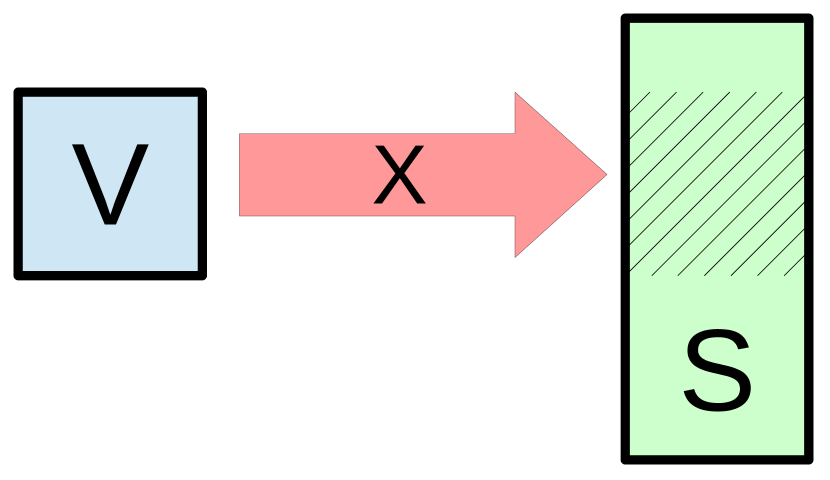
Figure 3: Lens viewing a region

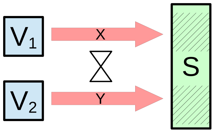
Figure 4: Independence

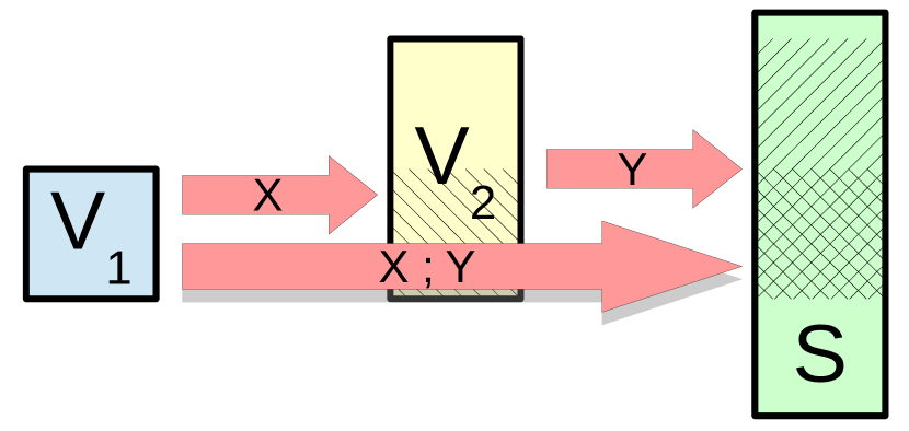
Figure 5: Lens composition

3.2 Axiomatic Basis

The use of lenses to model variables depends on get and put behaving according to a set of axioms.

Definition 3.5 (Total Lenses).

A total lens obeys the following axioms:

$$\textit{{get}}\,(\textit{{put}}\,s\,v) =v$$ (PutGet)

$$\textit{{put}}\,(\textit{{put}}\,s\,v^{\prime})\,v =\textit{{put}}\,s\,v$$ (PutPut)

$$\textit{{put}}\,s\,(\textit{{get}}\,s) =s$$ (GetPut)

We write $\mathcal{V}\Longmapsto\mathcal{S}$ for the set of total lenses with view type $\mathcal{V}$ and state space $\mathcal{S}$, and $\ast\Longmapsto\mathcal{S}$ for the set of total lenses with any view type, whose state space is $\mathcal{S}$.

We mechanise this algebraic structure in Isabelle using locales, following the pattern given by Ballarin [8]. Total lenses are usually called “very well-behaved” lenses [32, 31], but we believe “total” is more descriptive, since it is always possible to meaningfully project a view from a state. Axiom PutGet states that if a state has been constructed by application of $\textit{{put}}\,s\,v$, then a matching get returns the injected value, $v$. Axiom PutPut states that a later put overrides an earlier one, so that the previously injected value $v^{\prime}$ is replaced by $v$. Finally, Axiom GetPut states that for any state element $s$, if we extract the view element and then update the original using it, then we get precisely $s$ back.

We now demonstrate that every field of a record yields a total lens.

Lemma 3.6.

For any field $f_{i}$ of a record type $R$, the record lens $\hbox{{{{rec}}}}^{R}_{f_{i}}$ forms a total lens.

Proof.

For illustration, we prove each lens axiom in turn.

1. PutGet: $\textit{{get}}\,(\textit{{put}}\,s\,v)=f_{i}\,(s(f_{i}:=v))=v$

2. PutPut: $\textit{{put}}\,(\textit{{put}}\,s\,v^{\prime})\,v=(\mathop{\mathstrut{\lambda}}\nolimits s\,v@s(f_{i}:=v))\,(s(f_{i}:=v^{\prime}))\,v=(\mathop{\mathstrut{\lambda}}\nolimits v@s(f_{i}:=v^{\prime})(f_{i}:=v))\,v=\textit{{put}}\,s\,v$

3. GetPut: $\textit{{put}}\,s\,(\textit{{get}}\,s)=(\mathop{\mathstrut{\lambda}}\nolimits s\,v@s(f_{i}:=v))\,s\,(f_{i}\,s)=s(f_{i}:=f_{i}\,s)=s$

Consequently, the record lens is indeed a total lens. ∎

We can similarly show that fst, snd, and fun are total lenses.

Lemma 3.7.

For any $A$,$B$, and $k\in A$, $\textit{{{fst}}}^{A,B}$, $\textit{{{snd}}}^{A,B}$, and $\hbox{{{{fun}}}}^{A,B}_{k}$ are total lenses.

While both PutGet and PutPut are satisfied for most useful state-space models we can consider, this is not the case for GetPut. For example, if we consider a lens that projects the valuation of an element $x:A$ from a partial function $f:A\mathrel{\ooalign{\hfil$\mapstochar\mkern 5.0mu$\hfil\cr$\rightarrow$}}B$, then get is only meaningful when $x\in\mathop{\mathrm{dom}}(f)$. Since get is total, it must return a value, but this will be arbitrary and therefore placing it back into $f$ alters its domain. We do not consider lenses that do not satisfy GetPut in this paper, but simply observe that total lenses are a useful, though not universal solution for state space modelling.

3.3 Independence

So far we have considered the behaviour of individual lenses, but programs reference several variables and so it is necessary to compare them. One of the most important relationships between lenses is independence of their corresponding views, which is illustrated in Figure 5. We formally characterise independence below.

Definition 3.8 (Independent Lenses).

Lenses $X:\mathcal{V}_{1}\Longrightarrow\mathcal{S}$ and $Y:\mathcal{V}_{2}\Longrightarrow\mathcal{S}$ are independent, written $X\mathop{\,\bowtie\,}Y$, provided they satisfy the following laws:

$$\textit{{put}}_{X}\,(\textit{{put}}_{Y}\,s\,v)\,u \penalty 10000\ =\,\textit{{put}}_{Y}\,(\textit{{put}}_{X}\,s\,u)\,v$$ (LI1)

$$\textit{{get}}_{X}\,(\textit{{put}}_{Y}\,s\,v) \penalty 10000\ =\,\textit{{get}}_{X}\,s$$ (LI2)

$$\textit{{get}}_{Y}\,(\textit{{put}}_{X}\,s\,u) \penalty 10000\ =\,\textit{{get}}_{Y}\,s$$ (LI3)

Lenses $X$ and $Y$, which share the same state space but not necessarily the same view type, are independent provided that applications of their respective put functions commute (LI1), and their respective get functions are not influenced by the corresponding put functions (LI2, LI3). In the encoding of Example 2.3, we have that $x\mathop{\,\bowtie\,}y$, $x\mathop{\,\bowtie\,}hp$, and $y\mathop{\,\bowtie\,}hp$: these are distinct variables. Nevertheless, lens independence captures a deeper concept, since lenses with different types are not guaranteed to be independent, as they might represent a different view on the same region.

Independence can, for example, be used capture the condition for commutativity of assignments. If $x$ and $y$ are variables, then we can characterise the following law

$$(x:=e\mathrel{\hbox{\rm;}}y:=f)=(y:=f\mathrel{\hbox{\rm;}}x:=e)\text{\quad provided $x\mathop{\,\bowtie\,}y$, and $e$ and $f$ are constants}$$

which partly formalises Example 2.1. Such assignment laws will be explored further in Section 4. We can show that $\textit{{{fst}}}\mathop{\,\bowtie\,}\textit{{{snd}}}$ using the calculation below.

Lemma 3.9.

$\textit{{{fst}}}\mathop{\,\bowtie\,}\textit{{{snd}}}$

Proof.

We first prove that $\textit{{put}}_{\textit{{{fst}}}}$ commutes with $\textit{{put}}_{\textit{{{snd}}}}$ (LI1) by evaluation, assuming $s=(s_{1},s_{2})$:

$$\textit{{put}}_{\textit{{{fst}}}}(\textit{{put}}_{\textit{{{snd}}}}\,s\,v)\,u\,=\,\textit{{put}}_{\textit{{{fst}}}}(\textit{{put}}_{\textit{{{snd}}}}\,(s_{1},s_{2})\,v)\,u$$

$$=\,\, \textit{{put}}_{\textit{{{fst}}}}\,(s_{1},v)\,u\,=\,(u,v)\,=\,\textit{{put}}_{\textit{{{snd}}}}\,(u,s_{2})\,v$$

$$=\,\, \textit{{put}}_{\textit{{{snd}}}}\,(\textit{{put}}_{\textit{{{fst}}}}\,(s_{1},s_{2})\,u)\,v\,=\,\textit{{put}}_{\textit{{{snd}}}}\,(\textit{{put}}_{\textit{{{fst}}}}\,s\,u)\,v$$

Similarly, we can also prove LI2 by evaluation:

$$\textit{{get}}_{\textit{{{fst}}}}\,(\textit{{put}}_{\textit{{{snd}}}}\,s\,v)\,=\,\textit{{get}}_{\textit{{{fst}}}}\,(\textit{{put}}_{\textit{{{snd}}}}\,(s_{1},s_{2})\,v)\,=\,\textit{{get}}_{\textit{{{fst}}}}\,(s_{1},v)\,=\,s_{1}\,=\,\textit{{get}}_{\textit{{{fst}}}}\,(s_{1},s_{2})\,=\,\textit{{get}}_{\textit{{{fst}}}}\,s$$

Finally, LI3 follows by a symmetric proof. ∎

A further, illustrative result is the meaning of independence in the total function lens:

Lemma 3.10.

$\hbox{{{{fun}}}}_{a}\mathop{\,\bowtie\,}\hbox{{{{fun}}}}_{b}\mathrel{\Leftrightarrow}a\neq b$

Two instances of the total function lens are independent if, and only if, the parametrised inputs $a$ and $b$ are different. This reflects the intuition of a function – every input is associated with a distinct output.

We can actually show that axioms LI2 and LI3 in Definition 3.8 can be dispensed with when $X$ and $Y$ are both total lenses. Consequently, we can adopt a simpler definition of independence:

Theorem 3.11.

If lenses $X:\mathcal{V}_{1}\Longrightarrow\mathcal{S}$ and $Y:\mathcal{V}_{2}\Longrightarrow\mathcal{S}$ are both total then

$$X\mathop{\,\bowtie\,}Y\mathrel{\Leftrightarrow}\mathop{\mathstrut{\forall}}\nolimits(u,v,s)@\textit{{put}}_{X}\,(\textit{{put}}_{Y}\,s\,v)\,u\,=\,\textit{{put}}_{Y}\,(\textit{{put}}_{X}\,s\,u)\,v$$

However, the weaker definition of independence is still useful for the situation when not all three axioms of total lenses are satisfied [34].

3.4 Lens Combinators

Lenses can be independent, but they can also be ordered by containment using the sublens relation $X\preceq Y$, which orders lenses. The intuition is that $Y$ captures a larger region of the state space than $X$. One interpretation is a subset operator for relating lens sets. Before we can get to the definition of this $\preceq$, we first need to define some basic lens combinators.

Definition 3.12 (Basic Lenses).

$\mathbf{0}_{S}\,\triangleq\,\left\langle\{\emptyset\}\,\middle|\,S\,\middle|\,\mathop{\mathstrut{\lambda}}\nolimits s@\emptyset\,\middle|\,\mathop{\mathstrut{\lambda}}\nolimits s\,v@s\right\rangle\qquad\mathbf{1}_{S}\,\triangleq\,\left\langle S\,\middle|\,S\,\middle|\,\mathop{\mathstrut{\lambda}}\nolimits s@s\,\middle|\,\mathop{\mathstrut{\lambda}}\nolimits s\,v@v\right\rangle$

Lemma 3.13 (Basic Lenses Closure).

For any $S$, $\mathbf{0}_{S}$ and $\mathbf{1}_{S}$ are total lenses.

The $\mathbf{0}$ lens has a unitary view type, $\{\emptyset\}$. Consequently, for any element of the state space, it always views the same value $\emptyset$. It cannot be used to either observe or change a state, and it is therefore entirely ineffectual in nature. It can be interpreted as the empty set of lenses. Conversely, the $\mathbf{1}$ lens, with type $S\Longrightarrow S$, views the entirety of the state. It can be interpreted as the set of all lenses in the state space. We sometimes omit type information from these basic lenses when this can be inferred from the context.

It is useful in several circumstances to chain lenses together, provided that the view of one matches the source of the other. For this, we adopt the lens composition operator, originally defined by J. Foster [31].

Definition 3.14.

$X\fatsemi Y\,\,\triangleq\,\,\left\langle\mathcal{V}_{X}\,\middle|\,\mathcal{S}_{Y}\,\middle|\,\textit{{get}}_{X}\mathrel{\circ}\textit{{get}}_{Y}\,\middle|\,\mathop{\mathstrut{\lambda}}\nolimits s\,v@\textit{{put}}_{Y}\,s\,(\textit{{put}}_{X}\,(\textit{{get}}_{Y}\,s)\,v)\right\rangle\,\,\text{if }\mathcal{S}_{X}=\mathcal{V}_{Y}$

Lemma 3.15 (Composition Closure).

If $X$ and $Y$ are total lenses, then $X\fatsemi Y$ is a total lens.

A lens composition, $X\fatsemi Y$, for $X:A\Longrightarrow B$ and $Y:B\Longrightarrow C$ chains together two lenses. It is illustrated in Figure 5. When $X$ characterises an $A$-shaped region of $B$, and $Y$ characterises a $B$-shaped region of $C$, overall lens $X\fatsemi Y$ characterises an $A$-shaped region of $C$. It is useful when we have a state space composed of several individual state components, and we wish to select a variable of an individual component.

Example 3.16.

In an object oriented program we may have $m\in{\mathbb{N}}$ objects whose states are characterised by lenses $o_{i}:O_{i}\Longrightarrow\mathcal{S}$, for $i\in\{1..m\}$, where each $O_{i}$ characterises the respective object state. An object $o_{k}$ has $n\in{\mathbb{N}}$ attributes, characterised by lenses $x_{j}:\tau_{j}\Longrightarrow O_{k}$ for $j\in\{1..n\}$. We can select one of these attributes from the global state context by the composition $x_{j}\fatsemi o_{k}:\tau_{j}\Longrightarrow\mathcal{S}$. ∎

Composition is also useful for collections, such as the heap array in Example 2.3. If $hp:(addr\to{\mathbb{Z}})\Longrightarrow\mathcal{S}$, that is, a lens which views a function in $\mathcal{S}$, then we can represent a lookup, $hp[loc]$, by the composition $\hbox{{{{fun}}}}^{addr,{\mathbb{Z}}}_{loc}\fatsemi hp$.

Lens composition obeys a number of useful algebraic properties, as shown below.

Theorem 3.17 (Composition Laws).

If $X:A\Longrightarrow B$, $Y:B\Longrightarrow C$, and $Z:C\Longrightarrow D$ are total lenses then the following identities hold:

$$X\fatsemi(Y\fatsemi Z)\,\,=\,\,(X\fatsemi Y)\fatsemi Z\qquad X\fatsemi\mathbf{1}_{B}\,\,=\,\,\mathbf{1}_{A}\fatsemi X=X\qquad\mathbf{0}_{A}\fatsemi X\,\,=\,\,\mathbf{0}_{B}$$

Lens composition is associative, since the order in which lenses are composed is irrelevant, and it has $\mathbf{1}$ as its left and right units. Moreover, $\mathbf{0}$ is a left annihilator, since if the view is reduced to $\{\emptyset\}$ then no further data can be extracted.

While composition can be used to chain lenses in sequence, it is also possible to compose them in parallel, which is the purpose of the next operator.

Definition 3.18 (Lens Sum).

$$X+Y\,\,\triangleq\,\, \left\langle\mathcal{V}_{X}\times\mathcal{V}_{Y}\,\middle|\,\mathcal{S}_{X}\,\middle|\,\mathop{\mathstrut{\lambda}}\nolimits s@(\textit{{get}}_{X}\,s,\textit{{get}}_{Y}\,s)\,\middle|\,\mathop{\mathstrut{\lambda}}\nolimits s\,(v_{1},v_{2})@\textit{{put}}_{Y}\,(\textit{{put}}_{X}\,s\,v_{1})\,v_{2}\right\rangle \text{if }\mathcal{S}_{X}=\mathcal{S}_{Y}$$

Lens sum allows us to simultaneously manipulate two regions of $\mathcal{S}$, characterised by $X:\mathcal{V}_{1}\Longrightarrow\mathcal{S}$ and $Y:\mathcal{V}_{2}\Longrightarrow\mathcal{S}$. Consequently, the view type is the product of the two constituent views: $\mathcal{V}_{1}\times\mathcal{V}_{2}$. The get function applies both constituent get functions in parallel. The put function applies the constituent put functions, but in sequence since we are in the function domain. We can prove that total independent lenses are closed under lens sum.

Lemma 3.19 (Sum Closure).

If $X$ and $Y$ are independent total lenses, then $X+Y$ is a total lens.

We require that $X\mathop{\,\bowtie\,}Y$, since manipulation of two overlapping regions could have unexpected results, and then also the order of the put functions is irrelevant.

Lens sum can characterise independent concurrent views and updates to the state space. For example, we can encode a simultaneous update to two variables as $(x+y):=(e,f)$. Moreover, lens sum can also be used to characterise sets of independent lenses. If we model three variables using lenses $x$, $y$, and $z$ which share the same source and are all independent, then the set $\{x,y,z\}$ can be represented by $x+y+z$.

With the help of lens composition, we can now also prove some algebraic laws for lens sum.

Lemma 3.20.

If $X$ and $Y$ are independent total lenses then the following identities hold:

$$\textit{{{fst}}}\fatsemi(X+Y)\,=\,X\quad\textit{{{snd}}}\fatsemi(X+Y)\,=\,Y\quad(X+Y)\fatsemi Z\,=\,(X\fatsemi Z)+(Y\fatsemi Z)$$

The first two identities show that fst and snd composed with $+$ yield the left- and right-hand side lenses, respectively. If we perform a simultaneous update using $X+Y$, but then throw away one them by composing with fst and snd, then the result is simply $X$ or $Y$, respectively. The third identity shows that $\fatsemi$ distributes from the right through lens sum. It does not in general distribute from the left as such a construction is not well-formed. We next show some independence properties for the operators introduced so far.

Lemma 3.21 (Independence).

If $X$, $Y$, and $Z$ are total lenses then the following laws hold:

$$\mathbf{0}\mathop{\,\bowtie\,}X$$

$$X\mathop{\,\bowtie\,}Y\,\mathrel{\Leftrightarrow}\, Y\mathop{\,\bowtie\,}X$$

$$Y\mathop{\,\bowtie\,}Z\,\mathrel{\Rightarrow}\, (X\fatsemi Y)\mathop{\,\bowtie\,}Z$$

$$(X\fatsemi Z)\mathop{\,\bowtie\,}(Y\fatsemi Z)\,\mathrel{\Leftrightarrow}\, X\mathop{\,\bowtie\,}Y$$

$$X\mathop{\,\bowtie\,}Z\mathrel{\wedge}Y\mathop{\,\bowtie\,}Z\,\mathrel{\Rightarrow}\, (X+Y)\mathop{\,\bowtie\,}Z$$

The $\mathbf{0}$ lens is independent from any lens, since it views none of the state space. Lens independence is a symmetric relation, as expected. Lens composition preserves independence: if $Y\mathop{\,\bowtie\,}Z$ then composing $X$ with $Y$ still yields a lens independent of $Z$. Referring back to Example 2.3, if $x\mathop{\,\bowtie\,}hp$, then clearly also $x\mathop{\,\bowtie\,}hp[loc]$. $X$ and $Y$ composed with a common lens $Z$ are independent if, and only if, $X$ and $Y$ are themselves independent. Combining this with Lemma 3.10, we can deduce that $hp[l_{1}]$ and $hp[l_{2}]$ are independent if and only $l_{1}\neq l_{2}$. Finally, lens sum also preserves independence: if both $X$ and $Y$ are independent of $Z$, then also $X+Y$ is independent of $Z$. Thus, if $x\mathop{\,\bowtie\,}hp$ and $y\mathop{\,\bowtie\,}hp$, then also $x+y\mathop{\,\bowtie\,}hp$.

3.5 Observational Order and Equivalence

We recall that a lens $X$ can view a larger region than another lens $Y$, with the implication that $Y$ is fully dependent on $X$. For example, it is clear that in Example 3.16 each object fully possesses each of its attributes, and likewise each attribute lens $x_{j}\fatsemi o_{k}$ is fully dependent on lens $o_{k}$. We can formalise this using the lens order, $X\preceq Y$, which we can now finally define.

Definition 3.22 (Lens Order).

$(X\preceq Y)\triangleq(\mathcal{S}_{X}=\mathcal{S}_{Y}\mathrel{\wedge}(\mathop{\mathstrut{\exists}}\nolimits Z:\mathcal{V}_{X}\Longmapsto\mathcal{V}_{Y}@X=Z\fatsemi Y))$

A lens $X:V_{1}\Longrightarrow S$ is narrower than a lens $Y:V_{2}\Longrightarrow S$ provided that they share the same state space, and there exists a total lens $Z:V_{1}\Longmapsto V_{2}$, such that $X$ is the same as $Z\fatsemi Y$. In other words, the behaviour of $X$ is defined by firstly viewing the state using $Y$, and secondly viewing a subregion of this using $Z$. An order characterises the size of a lens’s aperture: how much of the state space a lens can view. For example, we can prove that $x_{j}\fatsemi o_{k}\preceq o_{k}$, by setting $Z=x_{j}$ in Definition 3.22. For the same reason, we can also show that $hp[loc]\preceq hp$. The lens order relation is a preorder, as demonstrated below.

Theorem 3.23.

For any $\mathcal{S}$, $(\ast\Longmapsto\mathcal{S},\preceq)$ forms a preorder, that is, $\preceq$ is reflexive and transitive. Furthermore, the least element of $\ast\Longmapsto\mathcal{S}$ is $\mathbf{0}_{\mathcal{S}}$, and the greatest element is $\mathbf{1}_{\mathcal{S}}$.

Clearly, $\mathbf{0}$ is the narrowest possible lens since it allows us to view nothing, and $\mathbf{1}$ is the widest lens, since it views the entire state. This is consistent with the intuition that $\mathbf{0}$ represents the empty set, $\mathbf{1}$ represents the set of all lenses, and $\preceq$ is a subset-like operator. We can prove the following intuitive theorem for sublenses.

Lemma 3.24.

If $X,Y$ are total lenses and $X\preceq Y$, then the following identities hold:

$$\textit{{put}}_{Y}\,(\textit{{put}}_{X}\,s\,v)\,u =\textit{{put}}_{Y}\,s\,u$$ (LS1)

$$\textit{{get}}_{X}\,(\textit{{put}}_{Y}\,s\,v) =\textit{{get}}_{X}\,(\textit{{put}}_{Y}\,s^{\prime}\,v)$$ (LS2)

Law LS1 is a generalisation of Axiom PutPut: a later $\textit{{put}}_{Y}$ overrides an earlier $\textit{{put}}_{X}$ when $X\preceq Y$. Law LS2 states that when viewing an update on $Y$ via a narrower lens $X$ we can ignore the valuation of the original state, since the update replaces all the relevant information. We can now use these results to prove a number of ordering lemmas for lens compositions.

Lemma 3.25 (Lens Order).

If $X$, $Y$, and $Z$ are total lenses then they satisfy the following laws:

$$X\fatsemi Y \preceq Y$$ (LO1)

$$X\preceq Y\mathrel{\wedge}Y\mathop{\,\bowtie\,}Z \mathrel{\Rightarrow}X\mathop{\,\bowtie\,}Z$$ (LO2)

$$X\mathop{\,\bowtie\,}Z\mathrel{\wedge}Y\preceq Z \mathrel{\Rightarrow}(X+Y)\preceq(X+Z)$$ (LO3)

$$X\mathop{\,\bowtie\,}Y \mathrel{\Rightarrow}X+Y\preceq Y+X$$ (LO4)

$$X\mathop{\,\bowtie\,}Y\mathrel{\wedge}X\mathop{\,\bowtie\,}Z\mathrel{\wedge}Y\mathop{\,\bowtie\,}Z \mathrel{\Rightarrow}X+(Y+Z)\preceq(X+Y)+Z$$ (LO5)

As we observed, composition of $X$ and $Y$ yields a narrower lens than $Y$ (LO1): $hp[loc]\preceq hp$. Independence is preserved by the ordering, since a subregion of a larger independent region is also clearly independent (LO2) – $hp[loc]\mathop{\,\bowtie\,}x$ when $hp\mathop{\,\bowtie\,}x$. Lens sum also preserves the ordering in its right-hand component (LO3). Moreover, lens sum is commutative with respect to $\preceq$ (LO4), and also associative, assuming appropriate independence properties (LO5). From these laws, and utilising the preorder theorems, we can prove various useful corollaries, such as

$$X\mathop{\,\bowtie\,}Y\mathrel{\Rightarrow}X\preceq(X+Y)$$

which shows that $X$ is narrower than $X+Y$: the latter is an upper bound. Thus, if we intuitively interpret $\preceq$ as $\subseteq$, then $+$ corresponds to $\cup$, and we can combine independent lens sets: $\{a,b\}\cup\{c,d\}=(a+b)+(c+d)$. We can also show that

$$X\preceq Z\mathrel{\wedge}Y\preceq Z\mathrel{\wedge}X\mathop{\,\bowtie\,}Y\mathrel{\Rightarrow}(X+Y)\preceq Z$$

which shows that sum provides the least upper bound: $\cup$ preserves $\subseteq$. Finally, we can also induce an equivalence relation on lenses using the lens order in the usual way:

Definition 3.26 (Lens Equivalence).

$(X\approx Y)\triangleq(X\preceq Y\mathrel{\wedge}Y\preceq X)$

We define $\approx$ as the cycle of a preorder, and consequently we can prove that it forms an equivalence relation.

Corollary 3.27 (Lens Equivalence Relation).

For any $\mathcal{S}$, $(\ast\Longmapsto\mathcal{S},\approx)$ forms a setoid, that is, $\approx$ is an equivalence relation on the set $\ast\Longmapsto\mathcal{S}$ – it is reflexive, symmetric, and transitive.

Proof.

Reflexivity and transitivity follow by Theorem 3.23, and symmetry follows by definition. ∎

Lens equivalence is a heterogeneously typed relation that is different from equality ($X=Y$), since it requires only that the two state spaces are the same, whilst the view types of $X$ and $Y$ can be different. Consequently, it can be used to compare lenses of different view types and show that two sets of lenses are isomorphic. This makes this relation much more useful for evaluating observational equivalence between two lenses that have apparently differing views, and yet characterise precisely the same region. For example, in general we cannot show that $x+y+z=z+y+x$, since these constructions have different view types: $\mathcal{V}_{x}\times\mathcal{V}_{y}\times\mathcal{V}_{z}$ and $\mathcal{V}_{z}\times\mathcal{V}_{y}\times\mathcal{V}_{x}$, respectively, and so the formula is not even type correct. We can, however, show that $x+y+z\approx z+y+x$. This is reflected by the following set of algebraic laws.

Theorem 3.28.

If $X$, $Y$, and $Z$ are all total lenses then they satisfy the following identities:

$$X+(Y+Z)\,\,\approx\,\, (X+Y)+Z \text{if }X\mathop{\,\bowtie\,}Y,X\mathop{\,\bowtie\,}Z,Y\mathop{\,\bowtie\,}Z$$

$$X+\mathbf{0}\,\,\approx\,\, X$$

$$X+Y\,\,\approx\,\, Y+X \text{if }X\mathop{\,\bowtie\,}Y$$

Lens summation is associative, has $\mathbf{0}$ as a unit, and commutative, modulo $\approx$, and assuming independence of the components, which is consistent with the lens set interpretation. Lenses thus form a partial commutative monoid [24], modulo $\approx$, also known as a separation algebra [19], where $X+Y$ is effectively defined only when $X\bowtie Y$. Independence corresponds with separation algebra’s “separateness” relation, which means that there is no overlap between two areas of memory. We can also use $\approx$ to determine whether two independent lenses, $X$ and $Y$, partition the entire state space using the identity $X+Y\approx\mathbf{1}$ [34]. Finally, we can prove the following additional properties of equivalence.

Theorem 3.29.

If $X_{1}$, $X_{2}$, $Y_{1}$, $Y_{2}$, and $Y$ are total lenses then the following laws hold:

• If $X_{1}\mathop{\,\bowtie\,}Y$ and $X_{1}\approx X_{2}$ then $X_{2}\mathop{\,\bowtie\,}Y$;

• If $X_{1}\approx X_{2}$, $Y_{1}\approx Y_{2}$, and $X_{1}\mathop{\,\bowtie\,}Y_{1}$ then $X_{1}+Y_{1}\approx X_{2}+Y_{2}$;

• If $\mathcal{S}_{X_{1}}=\mathcal{V}_{Y}$ and $X_{1}\approx X_{2}$ then $X_{1}\fatsemi Y\approx X_{2}\fatsemi Y$.

Independence is, as can be expected, preserved by equivalence. Equivalence is a congruence relation with respect to $+$, provided the summed lenses are independent. It is also a left congruence for lens composition. We can neither prove that it is a right congruence, nor find a counterexample.

3.6 Mechanised State Spaces

Lenses allow us to express provisos in laws with side conditions about variables. Manual construction of state spaces using the lens combinators is tedious and so we have implemented an Isabelle/HOL command for automatically creating a new state space with the following form:

$$\hbox{{{{alphabet}}}}\,[\alpha_{1},\cdots,\alpha_{k}]S=([\beta_{1},\cdots,\beta_{m}]T\,+)^{?}\,\,x_{1}:\tau_{1}\,\,\cdots\,\,x_{n}:\tau_{n}$$

We name the command alphabet, since it effectively allows the definition of a UTP alphabet (see Section 2.1), which in turn induces a state space. The command creates a new state space type $S$ with $k$ type parameters ($\alpha_{i}$, for $1\leq i\leq k$), optionally extending the parent state space $T$ with $m$ type parameters ($\beta_{i}$, for $1\leq i\leq m$), and creates a lens for each of the variables $x_{i}:\tau_{i}$. It can be used to describe a concrete state space for a program. For brevity, we often abbreviate the alphabet command by the syntax

$$[\alpha_{1},\cdots,\alpha_{k}]\,S\,\triangleq\,[\beta_{1},\cdots,\beta_{m}]T+\left[x_{1}:\tau_{1},\,\,\cdots\,\,,x_{n}:\tau_{n}\right]$$

when used in mathematical definitions. Internally, the command performs the following steps:

1. generates a record space type $S$ with $n$ fields, which optionally extends a parent state space $T$;

2. generates a lens $x_{i}$ for each of the fields using the record lens $\hbox{{{{rec}}}}^{R}_{x_{i}}$;

3. automatically proves that each lens $x_{i}$ is a total lens;

4. automatically proves an independence theorem $x_{i}\mathop{\,\bowtie\,}x_{j}$ for each pair $i,j\in\{1\cdots n\}$ such that $i\neq j$;

5. generates lenses $\hbox{{{{base}}}}_{S}$ and $\hbox{{{{more}}}}_{S}$ that characterise the “base part” and “extension part”, respectively;

6. automatically proves a number of independence and equivalence properties.

We now elaborate on each of these steps in detail.

The new record type S yields an auxiliary type $[\alpha_{1},\cdots,\alpha_{k},\phi]\textit{S-ext}$ with additional type parameter $\phi$ that characterises future extensions. In particular, the non-extended type $[\alpha_{1},\cdots,\alpha_{k}]S$ is characterised by $[\alpha_{1},\cdots,\alpha_{k},\textit{unit}]\textit{S-ext}$, where unit is a distinguished singleton type. This extensible record type is isomorphic to a product of three basic component types:

$$([\beta_{1},\cdots,\beta_{m}]T\times(\tau_{1}\times\cdots\times\tau_{n}))\times\phi$$

These characterise, respectively, the part of state space described by $T$, the part described by the $n$ additional fields, and the extension part $\phi$. In the case that the state space does not extend an existing type, we can set $[\beta_{1},\cdots,\beta_{m}]T=\textit{unit}$.

For each field, the command generates a lens $x_{i}:\tau_{i}\Longrightarrow[\alpha_{1},\cdots,\alpha_{k},\phi]\textit{S-ext}$ using the record lens, and proves total lens and independence theorems. Each of these lenses is polymorphic over $\phi$, so that they can be applied to the base type and any extension thereof, in the style of inheritance in object oriented data structures. As we show in §6, this polymorphism allows us to characterise a hierarchy of UTP theories.

In addition to the field lenses, we create two special total lenses:

• $\hbox{{{{base}}}}_{S}:[\alpha_{1},\cdots,\alpha_{k}]S\Longrightarrow[\alpha_{1},\cdots,\alpha_{k},\phi]\textit{S-ext}$, which characterises the base part; and

• $\hbox{{{{more}}}}_{S}:\phi\Longrightarrow[\alpha_{1},\cdots,\alpha_{k},\phi]\textit{S-ext}$, which characterises the extension part.

The base part consists of only the inherited fields and those added by $S$. We automatically prove a number of theorems about these special lenses:

• $\hbox{{{{base}}}}_{S}\mathop{\,\bowtie\,}\hbox{{{{more}}}}_{S}$: the base and extension parts are independent;

• $\hbox{{{{base}}}}_{S}+\hbox{{{{more}}}}_{S}\approx\mathbf{1}$: they partition the entire state space;

• for $i\in\{1\cdots n\}$, $x_{i}\preceq\hbox{{{{base}}}}_{S}$: each variable lens is part of the base;

• $\hbox{{{{base}}}}_{S}\approx\hbox{{{{base}}}}_{T}+\left(\sum_{i\in\{1\cdots n\}}x_{i}\right)$: the base is composed of the parent’s base and the variable lenses;

• $\hbox{{{{more}}}}_{T}\approx\left(\sum_{i\in\{1\cdots n\}}x_{i}\right)+\hbox{{{{more}}}}_{S}$: the parent’s extension is composed of the variable lenses and the child’s extension part.

These theorems can help support the Isabelle/UTP laws of programming, which we elaborate in the next section. We emphasise, though, that the alphabet command is not the only way to construct a state space with lenses, and nor do the results that follow depend on the use of this command. We could, for example, axiomatise a collection of lenses, including independence relations over an abstract state space type, following Schirmer and Wenzel [73]. However, the alphabet command is a convenient tool in many circumstances.

4 Mechanising the UTP Relational Calculus

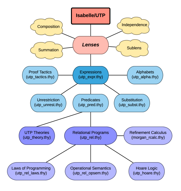
Figure 12: Main Isabelle/UTP Concepts and Theories

In this section we describe the core of Isabelle/UTP, including its expression model, meta-logical operators, predicate calculus, and relational calculus, building upon our algebraic model of state spaces. A direct result is an expressive model of relational programs which can be used in proving fundamental algebraic laws of programming [58], and for formal verification (§5). Moreover, the relational model is foundational to the mechanisation of UTP theories, and thus advanced computational paradigms, as we consider in §6. An overview of the Isabelle/UTP concepts and theories can be found in Fig. 12 at the end of the paper.

4.1 Expressions

Expressions are the basis of all other program and model objects in Isabelle/UTP, in that every such object is a specialisation of the expression type. An expression language typically includes literals, variables, and function symbols, all of which are also accounted for here. We model expressions as functions on the observation space: $[A,\mathcal{S}]\textit{{uexpr}}\cong(\mathcal{S}\to A)$, where $A$ is the return type, which is a standard shallow embedding approach [78, 6, 26]. However, lenses allow us to formulate syntax-like constraints, but without the need for deeply embedded expressions. A major advantage of this model is that we need not preconceive of all expression constructors, but can add them by definition.

We diverge from the standard shallow embedding approach, because we give explicit constructors for expressions. Usually shallow embeddings use syntax translations to transparently map between program expressions and the equivalent lifted expressions, for example,

$$e+(f-g)\leadsto\mathop{\mathstrut{\lambda}}\nolimits s@e(s)+(f(s)-g(s))$$

Here, we prefer to have expression constructors as first-class citizens.

Definition 4.1 (Expression Constructors).

Assume types $A$, $B$, $C$, and $\mathcal{S}$. We declare the constants:

$$\begin{array}[]{l}\textit{{var}}\,\colon(A\Longrightarrow\mathcal{S})\to[A,\mathcal{S}]\textit{{uexpr}}\\ \textit{{var}}\,x\triangleq\mathop{\mathstrut{\lambda}}\nolimits s@\textit{{get}}_{x}\,s\\[4.30554pt] \textit{{lit}}\,\colon A\Longrightarrow[A,\mathcal{S}]\textit{{uexpr}}\\ \textit{{lit}}\,k\triangleq\mathop{\mathstrut{\lambda}}\nolimits s@k\\[4.30554pt] \textit{{cond}}\,\colon[\mathbb{B},\mathcal{S}]\textit{{uexpr}}\to[A,\mathcal{S}]\textit{{uexpr}}\to[A,\mathcal{S}]\textit{{uexpr}}\to[A,\mathcal{S}]\textit{{uexpr}}\\ \textit{{cond}}\,b\,u_{1}\,u_{2}\triangleq\mathop{\mathstrut{\lambda}}\nolimits s@\mathsf{if}\,b(s)\,\mathsf{then}\,u_{1}(s)\,\mathsf{else}\,u_{2}(s)\\[4.30554pt] \textit{{uop}}\,\colon(A\!\to\!B)\to[A,\mathcal{S}]\textit{{uexpr}}\to[B,\mathcal{S}]\textit{{uexpr}}\\ \textit{{uop}}\,f\,u\triangleq\mathop{\mathstrut{\lambda}}\nolimits s@f(u(s))\\[4.30554pt] \textit{{bop}}\,\colon(A\!\to\!B\!\to\!C)\to[A,\mathcal{S}]\textit{{uexpr}}\to[B,\mathcal{S}]\textit{{uexpr}}\to[C,\mathcal{S}]\textit{{uexpr}}\\ \textit{{bop}}\,g\,u\,v\triangleq\mathop{\mathstrut{\lambda}}\nolimits s@g(u(s))\,(v(s))\end{array}$$

where $x:A\Longrightarrow\mathcal{S}$ is a lens; $k:A$ is a HOL constant; $f:A\to B$ and $g:A\to B\to C$ are functions; and $b:[\mathbb{B},\mathcal{S}]\textit{{uexpr}}$, $u,u_{1},u_{2}:[A,\mathcal{S}]\textit{{uexpr}}$, and $v:[B,\mathcal{S}]\textit{{uexpr}}$ are expressions.

The mechanisation of the core expression language is shown in Fig. 6, which uses Isabelle’s lifting package [60] to create each of the expression constructors. The operator $\textit{{var}}\,x$ is a variable expression, and returns the present value in the state characterised by lens $x$. For convenience, we assume that $x$, $y$, $z$, and decorations thereof, are lenses, and often use them directly as variable expressions without explicitly using var. We also use v to denote the $\mathbf{1}$ lens; this is effectively a special variable for the entire state.

The operator $\textit{{lit}}\,k$ represents a literal, or alternatively an arbitrary lifted HOL value, and corresponds to a constant function expression. We use the notation $\flqq k\frqq$ to denote a literal $k$. As well as lens-based variables, which are used to model program variables, expressions can also contain HOL variables, which are orthogonal and constant with respect to the program variables. HOL variables in literal constructions ($\flqq\textit{{x}}\frqq$) correspond to logical variables [61], also called “ghost variables”, which are important for verification [54, 61]. We use the notations x, y, and z to denote logical variables in expressions.

Operator $\textit{{cond}}\,b\,u_{1}\,u_{2}$ denotes a conditional expression; if $b$ is true then it returns $u_{1}$, otherwise $u_{2}$. It evaluates the boolean expression $b$ under the incoming state, and chooses the expression based on this. We use the notation $u_{1}\triangleleft b\triangleright u_{2}$ adopted in the UTP as a short hand for it.

Operators uop and bop lift HOL functions into the expression space by a pointwise lifting. With them we can transparently use HOL functions as UTP expression functions, for instance the summation $e+f$ is denoted by $\textit{{bop}}\,(+)\,e\,f$. Moreover, it is often possible to lift theorems from the underlying operators to the expressions themselves, which allows us to reuse the large library of HOL algebraic structures in Isabelle/UTP. For instance, if we know that $(A,+,0)$ is a monoid, then also we can show that for any $\mathcal{S}$, $([A,\mathcal{S}]\textit{{uexpr}},\textit{{bop}}\,(+),\textit{{lit}}\,0)$ forms a monoid. For convenience, we therefore often overload mathematically defined functions as expression constructs without further comment. In particular, we often overload $=$ as both equivalence of two expressions ($e=f$), and an expression of equality within an expression ($x=5$).

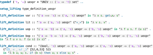
Figure 6: UTP Expression Model in Isabelle/HOL

This deep expression model allows us to mimick reasoning usually found in a deep embedding: the constructors above are like datatype constructs, but are really semantic definitions. We can then prove theorems about these constructs that allow us to reason in an inductive way, which is central to our approach to meta-logical reasoning. At the same time, we have developed a lifting parser in Isabelle/UTP, which allows automatic translation between HOL expressions and UTP expressions. We also have a tactic, rel-auto, that quickly and automatically eliminates the expression structure, resulting in a HOL expression.

The rel-auto tactic performs best when $\mathcal{S}$ is constructed using the alphabet command of §3.6, because we can enumerate all the field lenses. Given a state space $[x_{1}:\tau_{1},\cdots x_{n}\tau_{n}]$, we can eliminate the $s$ state space variable in a proof goal by replacing it with a tuple of logical variables ($\textit{{x}}_{1}\cdots\textit{{x}}_{n}$). This, in turn, means that we can eliminate each lens and replace it with a corresponding logical variable, for example:

$$(x+y)-z>3\leadsto(\textit{{x}}+\textit{{y}})-\textit{{z}}>3$$

The result is a simpler expression containing only logical variables, though of course with the loss of lens properties. This means that we have both the additional expressivity and fidelity afforded by lenses, and the proof automation of Isabelle/HOL.

4.2 Predicate Calculus

A predicate is an expression with a Boolean return type, $[\mathcal{S}]\textit{{upred}}\triangleq[\mathbb{B},\mathcal{S}]\textit{{uexpr}}$, so that predicates are a subtype of expressions. The majority of predicate calculus operators ($\neg$, $\mathrel{\wedge}$, $\mathrel{\vee}$, $\mathrel{\Rightarrow}$) are obtained by pointwise lifting of the equivalent operators in HOL. We also define the indexed operators $\bigwedge_{i\in A}\,P(i)$ and $\bigvee_{i\in A}\,P(i)$ similarly. The quantifiers are defined below. In order to notationally distinguish HOL from UTP operators, in the following definitions we subscript them with a H.

Definition 4.2 (Predicate Calculus Operators).

$$\mathop{\mathstrut{\exists}}\nolimits x@P \triangleq\mathop{\mathstrut{\lambda}}\nolimits s@\mathop{\mathstrut{\exists}}\nolimits_{\mbox{\tiny\sf H}}v:\mathcal{V}_{x}@P(\textit{{put}}_{x}\,s\,v)$$

$$\bm{\mathop{\mathstrut{\exists}}\nolimits}\textit{{x}}@P(\textit{{x}}) \triangleq\mathop{\mathstrut{\lambda}}\nolimits s@\mathop{\mathstrut{\exists}}\nolimits_{\mbox{\tiny\sf H}}\textit{{x}}@P(\textit{{x}})(s)$$

$$[P] \triangleq\mathop{\mathstrut{\forall}}\nolimits\hbox{{{{v}}}}@P$$

$$(P\mathrel{\sqsubseteq}Q) \triangleq(\mathop{\mathstrut{\forall}}\nolimits_{\mbox{\tiny\sf H}}s@(Q\mathrel{\Rightarrow}P)s)$$

Existential quantification over a lens $x$ quantifies possible values for the lens $v:\mathcal{V}_{x}$, and updates the state with this using put. Universal quantification is obtained by duality. The emboldened existential quantifier, $\bm{\mathop{\mathstrut{\exists}}\nolimits}$, quantifies a logical variable in a parametric predicate $P(\textit{{x}})$ by a direct lifting of the corresponding HOL quantifier. We emphasise that $\mathop{\mathstrut{\exists}}\nolimits$ and $\bm{\mathop{\mathstrut{\exists}}\nolimits}$ are semantically very different: in a lens quantification, $\mathop{\mathstrut{\exists}}\nolimits x@P$, the lens $x$ must be an existing lens or expression. This lens is not bound by the quantification, unlike $\bm{\mathop{\mathstrut{\exists}}\nolimits}\textit{{x}}@P(\textit{{x}})$ where x becomes a logical variable bound in $P$. Lens quantification is elsewhere called liberation [25, 22] since it removes any restrictions on the valuation of $x$.

The universal closure, $[P]$, universally quantifies every variable in the alphabet of $P$ using the state variable v. The refinement relation $P\mathrel{\sqsubseteq}Q$ is then defined as a HOL predicate, requiring that $Q$ implies $P$ in every state $s$.

Since the definitions are by lifting of the underlying HOL operators, we obtain the following theorem.

Theorem 4.3.

For any $\mathcal{S}$, $([\mathcal{S}]\textit{{upred}},\bigvee,\textit{{false}},\bigwedge,\textit{{true}},\neg)$ forms a complete Boolean algebra, that is:

• $([\mathcal{S}]\textit{{upred}},\mathrel{\vee},\textit{{false}},\mathrel{\wedge},\textit{{true}},\neg)$ is a Boolean algebra, and

• $([\mathcal{S}]\textit{{upred}},\mathrel{\sqsubseteq})$ is a complete lattice with infimum $\bigvee$, supremum $\bigwedge$, top element false, and bottom true.

As usual, via the Knaster-Tarski theorem, for any monotonic function $F:[\mathcal{S}]\textit{{upred}}\to[\mathcal{S}]\textit{{upred}}$ we can describe the least and greatest fixed points, $\mathop{\mathstrut{\mu}}\nolimits F$ and $\nu F$, which in UTP are called the weakest and strongest fixed points, and obey the usual fixed point laws. We can also algebraically characterise the UTP variable quantifiers using Cylindric Algebra [53], which axiomatises the quantifiers of first-order logic.

Theorem 4.4.

For any $\mathcal{S}$, $([\mathcal{S}]\textit{{upred}},\mathrel{\vee},\mathrel{\wedge},\neg,\textit{{false}},\textit{{true}},\mathop{\mathstrut{\exists}}\nolimits,=)$ forms a Cylindric Algebra, meaning that the following laws are satisfied for total lenses $x$, $y$, and $z$:

$$(\mathop{\mathstrut{\exists}}\nolimits x@\textit{{false}}) =\textit{{false}}$$ (C1)

$$(\mathop{\mathstrut{\exists}}\nolimits x@P) \mathrel{\sqsubseteq}P$$ (C2)

$$(\mathop{\mathstrut{\exists}}\nolimits x@(P\mathrel{\wedge}(\mathop{\mathstrut{\exists}}\nolimits x@Q))) =((\mathop{\mathstrut{\exists}}\nolimits x@P)\mathrel{\wedge}(\mathop{\mathstrut{\exists}}\nolimits x@Q))$$ (C3)

$$(\mathop{\mathstrut{\exists}}\nolimits x@\mathop{\mathstrut{\exists}}\nolimits y@P) =(\mathop{\mathstrut{\exists}}\nolimits y@\mathop{\mathstrut{\exists}}\nolimits x@P)$$ (C4)

$$(x=x) =\textit{{true}}$$ (C5)

$$(y=z) =(\mathop{\mathstrut{\exists}}\nolimits x@y=x\mathrel{\wedge}x=z) \textrm{if}\,x\mathop{\,\bowtie\,}y,x\mathop{\,\bowtie\,}z$$ (C6)

false $$=\left(\begin{array}[]{l}(\mathop{\mathstrut{\exists}}\nolimits x@x=y\mathrel{\wedge}P)\mathrel{\wedge}\\ (\mathop{\mathstrut{\exists}}\nolimits x@x=y\mathrel{\wedge}\neg P)\end{array}\right) \textrm{if}\,x\mathop{\,\bowtie\,}y$$ (C7)

From this algebra, the usual laws of quantification can be derived [53]. These laws illustrate the difference in expressive power between HOL and UTP variables. For the former, we cannot pose meta-logical questions like whether two variable names $x$ and $y$ refer to the same region, such as may be the case if they are aliased. For this kind of property, we can use lens independence $x\mathop{\,\bowtie\,}y$, as required by laws C6 and C7. We also prove the following laws for quantification.

Theorem 4.5.

If $A$ and $B$ are total lenses, then the following identities hold:

$$(\mathop{\mathstrut{\exists}}\nolimits A+B@P) =(\mathop{\mathstrut{\exists}}\nolimits A@\mathop{\mathstrut{\exists}}\nolimits B@P) \textrm{if}\,A\mathop{\,\bowtie\,}B$$ (Ex1)

$$(\mathop{\mathstrut{\exists}}\nolimits B@\mathop{\mathstrut{\exists}}\nolimits A@P) =(\mathop{\mathstrut{\exists}}\nolimits A@P) \textrm{if}\,B\preceq A$$ (Ex2)

$$(\mathop{\mathstrut{\exists}}\nolimits A@P) =(\mathop{\mathstrut{\exists}}\nolimits B@P) \textrm{if}\,A\approx B$$ (Ex3)

Here, lenses $A$ and $B$ can be interpreted as variable sets. Ex1 shows that quantifying over two disjoint sets of variables equates to quantification over both. Disjointness of variable sets is modelled by requiring that the corresponding lenses are independent. Ex2 shows that quantification over a larger lens subsumes a smaller lens. Finally Ex3 shows that if we quantify over two lenses that identify the same subregion then those two quantifications are equal. We now have a complete set of operators and laws for the predicate calculus.

4.3 Meta-Logic

Lenses treat variables as semantic objects that can be checked for independence, ordered, and composed in various ways. As we have noted, we can consider such manipulations as meta-logical with respect to the predicate. We add further specialised meta-logical queries for expressions.

Often we want to check which regions of the state space an expression depends on, for example to support laws of programming and verification calculi, like Example 2.1. In a deep embedding, this is characterised syntactically using free variables. However, lenses allow us to characterise a corresponding semantic notion called “unrestriction”, which is originally due to Oliveira et al. [66].

Definition 4.6 (Unrestriction).

$$\text{-}\mathop{\sharp}\text{-}\,\,:\,\,\, (A\Longrightarrow S)\to[B,S]\textit{{uexpr}}\to\mathbb{B}$$

$$(x\mathop{\sharp}e)\,\triangleq\,\, \left(\mathop{\mathstrut{\forall}}\nolimits(s,k)@e(\textit{{put}}_{x}\,s\,k)=e(s)\right)$$

Intuitively, lens $x$ is unrestricted in expression $e$, written $x\mathop{\sharp}e$, provided that $e$’s valuation does not depend on $x$. Specifically, the effect of $e$ evaluated under state $s$ is the same if we change the value of $x$. For example, $x\,\mathop{\sharp}\,(y+2>y)$ is true, provided that $x\mathop{\,\bowtie\,}y$, since the truth value of $y+2>y$ is unaffected by changing $x$. Unrestriction is a weaker notion than free variables: if $x$ is not free in $e$ then $x\mathop{\sharp}e$, but not the inverse. For example, $x\mathop{\sharp}\,(x=\textit{{true}}\mathrel{\vee}x=\textit{{false}})$ for $x:\mathbb{B}$ is true, since this expression is always true no matter the valuation of $x$. As we shall see, unrestriction is a sufficient notion to formalise the provisos for the laws of programming. Below are some key laws for establishing whether an expression is unrestricted by a variable.

Lemma 4.7 (Unrestriction Laws).

If $x$ and $y$ are total lenses, then the following laws hold:

—$P$   $x\mathop{\sharp}\textit{{lit}}\,k$

$x\mathop{\,\bowtie\,}y$     $x\mathop{\sharp}u$     $y\mathop{\sharp}u$        $(x+y)\mathop{\sharp}u$

$x\preceq y$   $x\mathop{\sharp}(\mathop{\mathstrut{\exists}}\nolimits y@P)$

$x\mathop{\,\bowtie\,}y$     $x\mathop{\sharp}P$     $x\mathop{\sharp}(\mathop{\mathstrut{\forall}}\nolimits y@P)$

These laws are formulated in the style of an inductive definition, but in reality they are a set of lemmas in Isabelle over our deep expression model. Expression $\textit{{lit}}\,k$ does not depend on the state since it always returns $k$: any lens $x$ is unrestricted. Any lens $y$ that is independent of $x$ is unrestricted $\textit{{var}}\,x$. The laws for uop and bop require simply that the component expressions have lens $x$ unrestricted. The $\mathbf{0}$ lens is unrestricted in any expression $u$, since it characterises none of the state space.

Unrestriction is preserved by the lens order $\preceq$. The summation of lenses $x$ and $y$ is unrestricted in $u$ provided that $x$ and $y$ are independent, and both are unrestricted in $u$. Again, we note that $+$ can effectively be used to group lenses in order to characterise a set of variables. Following a lens quantification over $y$, any sublens $x$ of $y$ becomes unrestricted. On the other hand, the restriction of any lens independent of $x$ is unchanged. The final two laws are the dual case for the universal lens quantification.

We can also prove the following correspondence between predicate unrestriction and quantification.

Lemma 4.8.

If $x$ is a total lens then $(x\mathop{\sharp}P)\mathrel{\Leftrightarrow}(\mathop{\mathstrut{\exists}}\nolimits x@P)=P$.

We can alternatively characterise unrestriction of $x$ by showing that quantifying over $x$ in $e$ has no effect (it is a fixed point), which is a well-known property from Cylindric Algebra [53] and also Liberation Algebra [25, 22]. Specifically, quantification liberates the lens $x$ so that it is free to take any value. Nevertheless, Lemma 4.8 cannot replace Definition 4.6, as it applies only if $P$ is a predicate, and not for an arbitrary expression. We can prove a number of useful corollaries for quantification.

Corollary 4.9.

If $x\mathop{\sharp}P$ then $(\mathop{\mathstrut{\exists}}\nolimits x@P)=P$ and $(\mathop{\mathstrut{\exists}}\nolimits x@P\mathrel{\wedge}Q)=(P\mathrel{\wedge}(\mathop{\mathstrut{\exists}}\nolimits x@Q))$.

The cases for universal quantification ($\mathop{\mathstrut{\forall}}\nolimits$) also hold by duality.

Aside from checking for use of variables, UTP theories often require that the state space of a predicate can be extended with additional variables. An example of this is the variable block operator that adds a new local variable. In Isabelle/UTP, alphabets are implicitly characterised by state-space types, rather than explicitly as sets of variables. Consequently, we perform alphabet extensions by manipulation of the underlying state space using lenses. We define the following operator to extend a state space.

Definition 4.10 (Alphabet Extrusion).

$$\text{-}\!\oplus\text{-}\,\,:\,\,\, [A,S_{1}]\textit{{uexpr}}\to(S_{1}\Longrightarrow S_{2})\to[A,S_{2}]\textit{{uexpr}}$$

$$e\oplus a\,\,\triangleq\,\, \left(\mathop{\mathstrut{\lambda}}\nolimits s@e(\textit{{get}}_{a}\,s)\right)$$

Alphabet extrusion, $e\oplus a$, uses the lens $a:S_{1}\Longrightarrow S_{2}$ to alter the state space of $e:[A,S_{1}]\textit{{uexpr}}$ to become $S_{2}$. The lens effectively describes how one state space can be embedded into another. The operator can be used either to extend a state space, or coerce it to an isomorphic one. For example, if we assume we have a state space composed of two sub-regions: $\mathcal{S}\triangleq A\times B$, then, a predicate $P:[A]\textit{{upred}}$, which acts on state space $A$, can be coerced to one acting on $\mathcal{S}$ by an alphabet extrusion: $P\oplus\textit{{{fst}}}:[\mathcal{S}]\textit{{upred}}$. Naturally, we know that the resulting predicate is unrestricted by the $B$ region.

Lemma 4.11 (Alphabet Extrusion Laws).

$$\begin{array}[]{rclrcl}\textit{{lit}}\,k\oplus a&=&\textit{{lit}}\,k&\quad\textit{{var}}\,x\oplus a&=&\textit{{var}}\,(x\fatsemi a)\\ \textit{{uop}}\,f\,u\oplus a&=&\textit{{uop}}\,f\,(u\oplus a)&\quad\textit{{bop}}\,g\,u\,v\oplus a&=&\textit{{bop}}\,g\,(u\oplus a)\,(v\oplus a)\end{array}$$

Alphabet extrusion has no effect on a literal expression, other than to change its type, because it refers to no lenses. A variable constructor has its lens augmented by composing it with the alphabet lens $a$. The extrusion simply distributes through unary and binary expressions.

4.4 Substitutions

Substitution is an operator for replacing a variable in an expression with another expression: $e[f/x]$. Like free variables, it is often considered as a meta-logical operator [46]. However, shallow embeddings can support a similar operator at the semantic level [46, 4], for which the substitution laws can be proved as theorems. Here, we generalise this using lenses, and treat substitutions as first-class citizens that can contain multiple variable mappings, and also conditional substitutions. This allows us to unify substitution and multiple variable assignment, which we demonstrate in Theorem 4.21 (LP4) and Corollary 4.24.

Substitutions can be modelled as total functions $\sigma,\rho:\mathcal{S}\to\mathcal{S}$ that transform an initial state to a final state. However, it is more intuitive to consider a substitution as a set of mappings from variables to expressions: $[x\mapsto_{\tiny{\textnormal{{s}}}}e,y\mapsto_{\tiny{\textnormal{{s}}}}f]$. The simplest substitution, $id\triangleq(\mathop{\mathstrut{\lambda}}\nolimits x@x)$, leaves the state unchanged. We define operators for querying and updating our semantic substitution objects below.

Definition 4.12 (Substitution Query and Update).

$$\langle\sigma\rangle_{\tiny{\textnormal{{s}}}}\,x\,\triangleq\,(\mathop{\mathstrut{\lambda}}\nolimits s@\textit{{get}}_{x}\,(\sigma(s)))\qquad\sigma(x\mapsto_{\tiny{\textnormal{{s}}}}e)\,\triangleq\,(\mathop{\mathstrut{\lambda}}\nolimits s@\textit{{put}}_{x}\,(\sigma(s))\,(e(s)))$$

Substitution query $\langle\sigma\rangle_{\tiny{\textnormal{{s}}}}\,x:[A,\mathcal{S}]\textit{{uexpr}}$ returns the expression associated with $x:A\Longrightarrow\mathcal{S}$ in $\sigma:\mathcal{S}\to\mathcal{S}$ by composition of the latter with $\textit{{get}}_{x}$. Substitution update assigns the expression $e:[A,\mathcal{S}]\textit{{uexpr}}$ to the lens $x$ in $\sigma$. The definition constructs a function of type $\mathcal{S}\to\mathcal{S}$ that inputs the state $s$, evaluates $e$ with respect to $s$, calculates the state space updated by $\sigma$, and then uses put to update the value of $x$ in $\sigma(s)$ with the evaluated expression. We can then introduce the short-hands

$$\sigma(x_{1}\mapsto_{\tiny{\textnormal{{s}}}}e_{1},\cdots,x_{n}\mapsto_{\tiny{\textnormal{{s}}}}e_{n}) \triangleq(x_{1}\mapsto_{\tiny{\textnormal{{s}}}}e_{1})\cdots(x_{n}\mapsto_{\tiny{\textnormal{{s}}}}e_{n})$$

$$[x_{1}\mapsto_{\tiny{\textnormal{{s}}}}e_{1},\cdots,x_{n}\mapsto_{\tiny{\textnormal{{s}}}}e_{n}] \triangleq id(x_{1}\mapsto_{\tiny{\textnormal{{s}}}}e_{1},\cdots,x_{n}\mapsto_{\tiny{\textnormal{{s}}}}e_{n})$$

which, respectively, update a substitution $\sigma$ in $n$ variables by assigning $e_{i}$ to each variable $x_{i}$, and construct a new substitution from a set of maplets. If we have $x_{i}\mathop{\,\bowtie\,}x_{j}$ for each such variable, then these updates are effectively concurrent, regardless of the expressions. Otherwise, a syntactically later assignment ($x_{j}$) can override an earlier one ($x_{i}$ with $i<j$). This allows us to model multiple variable assignment, and also evaluation contexts for programs and expressions.

We also prove a number of laws about substitutions constructed from maplets.

Lemma 4.13.

If $x$ and $y$ are total lenses, then the following identities hold:

$$\langle\sigma(x\mapsto_{\tiny{\textnormal{{s}}}}e)\rangle_{\tiny{\textnormal{{s}}}}\,x =e$$ (SB1)

$$\sigma(x\mapsto_{\tiny{\textnormal{{s}}}}\langle\sigma\rangle_{\tiny{\textnormal{{s}}}}\,x) =\sigma$$ (SB2)

$$[x\mapsto_{\tiny{\textnormal{{s}}}}x] =id$$ (SB3)

$$\sigma(x\mapsto_{\tiny{\textnormal{{s}}}}e,y\mapsto_{\tiny{\textnormal{{s}}}}f) =\sigma(y\mapsto_{\tiny{\textnormal{{s}}}}f,x\mapsto_{\tiny{\textnormal{{s}}}}e) \textnormal{if }x\mathop{\,\bowtie\,}y$$ (SB4)

$$\sigma(x\mapsto_{\tiny{\textnormal{{s}}}}e,y\mapsto_{\tiny{\textnormal{{s}}}}f) =\sigma(y\mapsto_{\tiny{\textnormal{{s}}}}f) \textnormal{if }x\preceq y$$ (SB5)

Law SB1 states that looking up $x$ in a constructed substitution returns its associated expression, $e$. It essentially follows from lens axiom PutGet. Law SB2 is an $\eta$-conversion principle, which follows from GetPut. Law SB3 states that updating a variable to itself has no effect. Law SB4 states that two substitution maplets, $x\mapsto_{\tiny{\textnormal{{s}}}}e$ and $y\mapsto_{\tiny{\textnormal{{s}}}}f$, commute provided that $x$ and $y$ are independent. Similarly, SB5 states that a later assignment for $y$ overrides an earlier assignment for $x$ when $y$ is a wider lens than $x$. This is, of course, true in particular when $x=y$, which reduces to lens axiom PutPut.

Substitutions can be composed in sequence using function composition. Conditional substitutions can be expressed using the following construct.

Definition 4.14 (Conditional Substitution).

$\sigma\blacktriangleleft b\blacktriangleright\rho\,\triangleq\,(\mathop{\mathstrut{\lambda}}\nolimits s@\mathsf{if}\,b(s)\,\mathsf{then}\,\sigma(s)\,\mathsf{else}\,\rho(s))$.

A conditional substitution is equivalent to $\sigma$ when $b$ is true, and $\rho$ otherwise. The definition evaluates $b$ under the incoming state $s$, and then chooses which substitution to apply based on this. Substitutions can be applied to an expression using the following operator.

Definition 4.15 (Substitution Application).

$$-\!\mathop{\dagger}\!- \penalty 10000\ \colon(\mathcal{S}\to\mathcal{S})\to[A,\mathcal{S}]\textit{{uexpr}}\to[A,\mathcal{S}]\textit{{uexpr}}$$

$$\sigma\mathop{\dagger}e \triangleq(\mathop{\mathstrut{\lambda}}\nolimits s@e(\sigma(s)))$$

Application of a substitution $\sigma$ to an expression $e$ simply evaluates $e$ in the context of state $\sigma(s)$. We can also model the classical syntax for substitution, $P[v/x]\triangleq[x\mapsto_{\tiny{\textnormal{{s}}}}v]\mathop{\dagger}P$, and prove the substitution laws [4].

Lemma 4.16 (Substitution Application Laws).

$$\sigma\mathop{\dagger}\textit{{var}}\,x =\langle\sigma\rangle_{\tiny{\textnormal{{s}}}}\,x$$ (SA1)

$$\sigma(x\mapsto_{\textnormal{{s}}}e)\mathop{\dagger}u =\sigma\mathop{\dagger}u \textnormal{if }x\mathop{\sharp}u$$ (SA2)

$$\sigma\mathop{\dagger}\textit{{uop}}\,f\,v =\textit{{uop}}\,f\,(\sigma\mathop{\dagger}v)$$ (SA3)

$$\sigma\mathop{\dagger}\textit{{bop}}\,f\,u\,v =\textit{{bop}}\,f\,(\sigma\mathop{\dagger}u)\,(\sigma\mathop{\dagger}v)$$ (SA4)

$$(\mathop{\mathstrut{\exists}}\nolimits y@P)[e/x] =(\mathop{\mathstrut{\exists}}\nolimits y@P[e/x]) \textrm{if}\,x\mathop{\,\bowtie\,}y,y\mathop{\sharp}e$$ (SA5)

$$id\mathop{\dagger}e =e$$ (SA6)

$$\sigma\mathop{\dagger}\rho\mathop{\dagger}e =(\rho\mathrel{\circ}\sigma)\mathop{\dagger}e$$ (SA7)

$$\rho(x\mapsto_{\tiny{\textnormal{{s}}}}e)\mathrel{\circ}\sigma =(\rho\mathrel{\circ}\sigma)(x\mapsto_{\tiny{\textnormal{{s}}}}\sigma\mathop{\dagger}e)$$ (SA8)

$$\sigma(x\mapsto_{\tiny{\textnormal{{s}}}}e)\blacktriangleleft b\blacktriangleright\rho(x\mapsto_{\tiny{\textnormal{{s}}}}f) =(\sigma\blacktriangleleft b\blacktriangleright\rho)(x\mapsto_{\tiny{\textnormal{{s}}}}(e\triangleleft b\triangleright f))$$ (SA9)

Application of $\sigma$ to a variable $x$ is the valuation of $x$ in $\sigma$ (SA1). A substitution maplet for an unrestricted variable can be removed (SA2). Substitutions distribute through both unary (SA3) and binary (SA4) operators. A singleton substitution for variable $x$ can pass through an existential quantification over $y$ provided that $x$ and $y$ are independent, and $e$ is unrestricted by $y$ (SA5), which prevents variable capture. Application of $id$ has no effect (SA6), and application of two substitutions can be expressed by their composition (SA7). SA8 shows that when $\sigma$ is composed with another substitution composed of maplets ($x\mapsto_{\tiny{\textnormal{{s}}}}e$), it is simply applied to the expression $e$ of every such maplet. SA9 shows how two substitutions with matching maplets can be conditionally composed, by distributing the conditional.

We can also use substitutition and unrestriction to prove the one-point law [50] from predicate calculus, as employed in Hehner’s classic textbook on predicative programming [51].

Theorem 4.17.

If $x$ is a total lens and $x\mathop{\sharp}e$ then $(\mathop{\mathstrut{\exists}}\nolimits x@P\mathrel{\wedge}x=e)=P[e/x]$

As for expressions, we define an operator to extend the alphabet of a substitution.

Definition 4.18 (Substitution Alphabet Extrusion).

$\sigma\mathop{\oplus_{\mbox{\tiny{{s}}}}}a\,\triangleq\,(\mathop{\mathstrut{\lambda}}\nolimits s@\textit{{put}}_{a}\,s\,(\sigma(\textit{{get}}_{a}\,s)))$

We use the lens $a:S_{1}\Longrightarrow S_{2}$ to coerce $\sigma:S_{1}\to S_{1}$ to the state space $S_{2}$. The resulting substitution first obtains an element of $S_{1}$ from the incoming state $s:S_{2}$ using $\textit{{get}}_{a}$, applies the substitution to this, and then places the updated state back into $s$ using $\textit{{put}}_{a}$. This is the essence of a framed computation; the parts of $s$ outside of the view of $a$ are unchanged.

4.5 Relational Programs

A relation is a predicate on a product space $\mathcal{S}_{1}\times\mathcal{S}_{2}$, specifically, where $\mathcal{S}_{1}$ and $\mathcal{S}_{2}$ are the state spaces before and after execution, respectively. All laws that have been proved for expressions and predicates therefore hold for relations. We define types for both heterogeneous relations, $[\mathcal{S}_{1},\mathcal{S}_{2}]\textit{{urel}}\triangleq[\mathcal{S}_{1}\times\mathcal{S}_{2}]\textit{{upred}}$, and homogeneous relations $[\mathcal{S}]\textit{{hrel}}\triangleq[\mathcal{S},\mathcal{S}]\textit{{urel}}$. Operators true and false can be specialised in this relational setting, and stand for the most and least non-deterministic relations. Due to their special role, we use the notation true and false to explicitly refer to these relational counterparts.

In common with formal languages like Z [75] and B [1], UTP [57] uses the notational convention for variables that $x$ is the initial value and $x^{\prime}$ is its final value. The former can be denoted by the lens composition $x\fatsemi\textit{{{fst}}}$, and the latter by $x\fatsemi\textit{{{snd}}}$, where $x$ is actually the name of a lens of type $\tau\Longrightarrow\mathcal{S}$. In this presentation we define the operators below for lifting variables, expressions, and substitutions into the product space.

Definition 4.19 (Pre- and Postcondition Lifting).

$$x^{\mbox{\!\! $\blacktriangleleft$}}\triangleq x\fatsemi\textit{{{fst}}}\qquad x^{\mbox{\!\! $\blacktriangleright$}}\triangleq x\fatsemi\textit{{{snd}}}\qquad e^{\mbox{\!\! $\blacktriangleleft$}}\triangleq e\oplus\textit{{{fst}}}\qquad e^{\mbox{\!\! $\blacktriangleright$}}\triangleq e\oplus\textit{{{snd}}}\qquad\sigma^{\mbox{\!\! $\blacktriangleleft$}}\triangleq\sigma\mathop{\oplus_{\mbox{\tiny{{s}}}}}\textit{{{fst}}}\qquad\sigma^{\mbox{\!\! $\blacktriangleright$}}\triangleq\sigma\mathop{\oplus_{\mbox{\tiny{{s}}}}}\textit{{{snd}}}$$

The ${}^{\mbox{\!\! $\blacktriangleleft$}}$ and ${}^{\mbox{\!\! $\blacktriangleright$}}$ lift a lens, expression, or substitution, into the first and second components of a product state space $\mathcal{S}_{1}\times\mathcal{S}_{2}$. We deviate from the standard notation to avoid the ambiguity between “$x$” meaning an expression variable or an initial relational variable. Operator $e^{\mbox{\!\! $\blacktriangleleft$}}$ lifts an expression $e:[A,\mathcal{S}_{1}]\textit{{uexpr}}$ to an expression on the product state space $\mathcal{S}_{1}\times\mathcal{S}_{2}$, for any given $\mathcal{S}_{2}$. If $e$ is a predicate on the state variables, then $e^{\mbox{\!\! $\blacktriangleleft$}}$ is a predicate on the initial state, that is a precondition. Similarly, $e^{\mbox{\!\! $\blacktriangleright$}}$ constructs a postcondition with state space $\mathcal{S}_{1}\times\mathcal{S}_{2}$ from $e:[A,\mathcal{S}_{2}]\textit{{uexpr}}$. The analogous operators $\sigma^{\mbox{\!\! $\blacktriangleleft$}}$ and $\sigma^{\mbox{\!\! $\blacktriangleright$}}$ lift a substitution to the product space.

We can now define the main programming operators of the relational calculus.

Definition 4.20 (Programming Operators).

$$(P\mathrel{\hbox{\rm;}}Q) \penalty 10000\ \triangleq\,(\bm{\mathop{\mathstrut{\exists}}\nolimits}\textit{{v}}_{0}@P[\textit{{v}}_{0}/\hbox{{{{v}}}}^{\mbox{\!\! $\blacktriangleright$}}]\mathrel{\wedge}Q[\textit{{v}}_{0}/\hbox{{{{v}}}}^{\mbox{\!\! $\blacktriangleleft$}}])$$

I I $$\penalty 10000\ \triangleq\,(\hbox{{{{v}}}}^{\mbox{\!\! $\blacktriangleright$}}=\hbox{{{{v}}}}^{\mbox{\!\! $\blacktriangleleft$}})$$

$$\left\langle\sigma\right\rangle \penalty 10000\ \triangleq\,(\hbox{{{{v}}}}^{\mbox{\!\! $\blacktriangleright$}}=\sigma(\hbox{{{{v}}}}^{\mbox{\!\! $\blacktriangleleft$}}))$$

$$P\mathop{\hbox{\raisebox{0.0pt}{$\leftslice$}}}b\mathop{\hbox{\raisebox{0.0pt}{$\rightslice$}}}Q \penalty 10000\ \triangleq\,(b^{\mbox{\!\! $\blacktriangleleft$}}\mathrel{\wedge}P)\mathrel{\vee}(\neg b^{\mbox{\!\! $\blacktriangleleft$}}\mathrel{\wedge}Q)$$

$$b\oast Q \penalty 10000\ \triangleq\,\nu X@P\mathrel{\hbox{\rm;}}X\mathop{\hbox{\raisebox{0.0pt}{$\leftslice$}}}b\mathop{\hbox{\raisebox{0.0pt}{$\rightslice$}}}{\hbox{{I \kern-8.5ptI}}}$$

These broadly follow the common definitions given in relational calculus and the UTP book [57], but with subtle differences due to our use of lenses. Relational composition $P\mathrel{\hbox{\rm;}}Q$ existentiality quantifies a logical variable $\textit{{v}}_{0}$ that stands for the intermediate state between $P$ and $Q$. It is substituted as the final state of $P$ (using $\hbox{{{{v}}}}^{\mbox{\!\! $\blacktriangleright$}}$), and the initial state of $Q$; the resulting predicates are then conjoined. This definition yields a homogeneous composition operator, though in Isabelle/UTP composition is heterogeneous and has type $[\mathcal{S}_{1},\mathcal{S}_{2}]\textit{{urel}}\to[\mathcal{S}_{2},\mathcal{S}_{3}]\textit{{urel}}\to[\mathcal{S}_{1},\mathcal{S}_{3}]\textit{{urel}}$.

Relational identity (I I), or skip, equates the initial state with the final state, leaving all variables unchanged. $\left\langle\sigma\right\rangle$ is a generalised assignment operator, originally proposed by Back and von Wright [6, page 2] using a substitution $\sigma:\mathcal{S}\to\mathcal{S}$. Its definition states that the final state is equal to the initial state with $\sigma$ applied. The substitution $\sigma$ can be constructed as a set of maplets, so that a singleton assignment $x:=v$ can be expressed as $\left\langle x\mapsto_{\tiny{\textnormal{{s}}}}v\right\rangle$, and a multiple variable assignment as $\left\langle x_{1}\mapsto_{\tiny{\textnormal{{s}}}}v_{1},\cdots,x_{n}\mapsto_{\tiny{\textnormal{{s}}}}v_{n}\right\rangle$. Since $x$ can be any lens in an assignment, we can use it to assign any part of the state hierarchy that can be so characterised, for example an element of the heap (Example 2.3) or the attribute of an object (Example 3.16).

Conditional $P\mathop{\hbox{\raisebox{0.0pt}{$\leftslice$}}}b\mathop{\hbox{\raisebox{0.0pt}{$\rightslice$}}}Q$ states that if $b$ is true then behave like $P$, otherwise behave like $Q$. In the UTP book [57] the fact that $b$ acts on initial variables is a syntactic convention, whereas here this wellformedness condition is imposed by construction using $b^{\mbox{\!\! $\blacktriangleleft$}}$. For completeness, we use this operator, and the fact that all predicates, including relations, form a complete lattice, to define the while loop operator $b\oast P$. We use the strongest fixed-point, $\nu$, since we use it for partial correctness verification in §5.

We now have all the operators of a simple imperative programming language, and can prove the laws of programming [58, 57], but with a generalised presentation.

Theorem 4.21 (Generalised Laws of Programming).

$$(P\mathrel{\hbox{\rm;}}Q)\mathrel{\hbox{\rm;}}R =P\mathrel{\hbox{\rm;}}(Q\mathrel{\hbox{\rm;}}R)$$ (LP1)

$${\hbox{{I \kern-8.5ptI}}}\mathrel{\hbox{\rm;}}P =P\mathrel{\hbox{\rm;}}{\hbox{{I \kern-8.5ptI}}}=P$$ (LP2)

$$\hbox{{{{false}}}}\mathrel{\hbox{\rm;}}P =P\mathrel{\hbox{\rm;}}\hbox{{{{false}}}}=\hbox{{{{false}}}}$$ (LP3)

$$\left\langle\sigma\right\rangle\mathrel{\hbox{\rm;}}P =\sigma^{\mbox{\!\! $\blacktriangleleft$}}\mathop{\dagger}P$$ (LP4)

$$\left\langle\sigma\right\rangle\mathop{\hbox{\raisebox{0.0pt}{$\leftslice$}}}b\mathop{\hbox{\raisebox{0.0pt}{$\rightslice$}}}\left\langle\rho\right\rangle =\left\langle\sigma\blacktriangleleft b\blacktriangleright\rho\right\rangle$$ (LP5)

$$(P\mathrel{\hbox{\rm;}}(b\oast P))\mathop{\hbox{\raisebox{0.0pt}{$\leftslice$}}}b\mathop{\hbox{\raisebox{0.0pt}{$\rightslice$}}}{\hbox{{I \kern-8.5ptI}}}\, =b\oast P$$ (LP6)

$$P\mathop{\hbox{\raisebox{0.0pt}{$\leftslice$}}}\textit{{true}}\mathop{\hbox{\raisebox{0.0pt}{$\rightslice$}}}Q =P$$ (LP7)

$$P\mathop{\hbox{\raisebox{0.0pt}{$\leftslice$}}}\textit{{false}}\mathop{\hbox{\raisebox{0.0pt}{$\rightslice$}}}Q =Q$$ (LP8)

$$P\mathop{\hbox{\raisebox{0.0pt}{$\leftslice$}}}\neg b\mathop{\hbox{\raisebox{0.0pt}{$\rightslice$}}}Q =Q\mathop{\hbox{\raisebox{0.0pt}{$\leftslice$}}}b\mathop{\hbox{\raisebox{0.0pt}{$\rightslice$}}}P$$ (LP9)

$$(P\mathop{\hbox{\raisebox{0.0pt}{$\leftslice$}}}b\mathop{\hbox{\raisebox{0.0pt}{$\rightslice$}}}Q)\mathrel{\hbox{\rm;}}R =(P\mathrel{\hbox{\rm;}}R)\mathop{\hbox{\raisebox{0.0pt}{$\leftslice$}}}b\mathop{\hbox{\raisebox{0.0pt}{$\rightslice$}}}(P\mathrel{\hbox{\rm;}}R)$$ (LP10)

The majority of these are standard, and therefore we select only a few for commentary. LP4 is a generalisation of the forward assignment law: an assignment by $\sigma$ followed by relation $P$ is equivalent to $\sigma$ applied to the initial variables of $P$. The more traditional formulation [58, 57], $x:=e\mathrel{\hbox{\rm;}}P=P[e/x]$, is an instance of this law. Similarly, LP5 is a generalised conditional assignment law which combines $\sigma$ and $\rho$ into a single conditional substitution. All the other assignment laws can be proved, but we need some additional properties for relational substitutions, which are shown below. LP10 would normally require as a proviso that $b$ is an expression in initial variables only, but in our setting this fact follows by construction.

Lemma 4.22 (Relational Substitutions and Assignment).

$$\sigma^{\mbox{\!\! $\blacktriangleleft$}}\mathop{\dagger}(P\mathrel{\hbox{\rm;}}Q) =(\sigma^{\mbox{\!\! $\blacktriangleleft$}}\mathop{\dagger}P)\mathrel{\hbox{\rm;}}Q$$ (RS1)

$$\sigma^{\mbox{\!\! $\blacktriangleright$}}\mathop{\dagger}(P\mathrel{\hbox{\rm;}}Q) =P\mathrel{\hbox{\rm;}}(\sigma^{\mbox{\!\! $\blacktriangleright$}}\mathop{\dagger}Q)$$ (RS2)

$$\sigma^{\mbox{\!\! $\blacktriangleleft$}}\mathop{\dagger}\left\langle\rho\right\rangle =\left\langle\rho\mathrel{\circ}\sigma\right\rangle$$ (RS3)

$$\sigma^{\mbox{\!\! $\blacktriangleleft$}}\mathop{\dagger}(P\mathop{\hbox{\raisebox{0.0pt}{$\leftslice$}}}b\mathop{\hbox{\raisebox{0.0pt}{$\rightslice$}}}Q) =(\sigma^{\mbox{\!\! $\blacktriangleleft$}}\mathop{\dagger}P)\mathop{\hbox{\raisebox{0.0pt}{$\leftslice$}}}\,(\sigma\mathop{\dagger}b)\,\mathop{\hbox{\raisebox{0.0pt}{$\rightslice$}}}(\sigma^{\mbox{\!\! $\blacktriangleleft$}}\mathop{\dagger}Q)$$ (RS4)

RS1 shows that a precondition substitution applies only to the first element of a sequential composition, and RS2 is its dual. RS3 shows that precondition substitution applied to an assignment can be expressed as a composite assignment. RS4 shows that $\sigma^{\mbox{\!\! $\blacktriangleleft$}}$ applied to a conditional distributes through all three arguments. The precondition annotation is removed when applied to $b$ since this is a precondition expression already. Combining Theorem 4.21 with Lemma 4.22 we can prove the following corollaries of generalised assignment.

Corollary 4.23.

$\left\langle id\right\rangle={\hbox{{I \kern-8.5ptI}}}\qquad\left\langle\sigma\right\rangle\mathrel{\hbox{\rm;}}\left\langle\rho\right\rangle=\left\langle\rho\mathrel{\circ}\sigma\right\rangle\qquad\left\langle\sigma\right\rangle\mathrel{\hbox{\rm;}}(P\mathop{\hbox{\raisebox{0.0pt}{$\leftslice$}}}b\mathop{\hbox{\raisebox{0.0pt}{$\rightslice$}}}Q)=(\left\langle\sigma\right\rangle\mathrel{\hbox{\rm;}}P)\mathop{\hbox{\raisebox{0.0pt}{$\leftslice$}}}\sigma\mathop{\dagger}b\mathop{\hbox{\raisebox{0.0pt}{$\rightslice$}}}(\left\langle\sigma\right\rangle\mathrel{\hbox{\rm;}}Q)$

Moreover, with Lemma 4.16, Theorem 4.21, and Lemma 4.22 we can prove the classical assignment laws [58].

Corollary 4.24 (Assignment Laws).

$$x:=e\mathrel{\hbox{\rm;}}y:=f \penalty 10000\ =\,x,y:=e,f[e/x]$$

$$x:=x \penalty 10000\ =\,{\hbox{{I \kern-8.5ptI}}}$$

$$x,y:=e,y \penalty 10000\ =\,x:=e$$

$$x,y,z:=e,f,g \penalty 10000\ =\,y,x,z:=f,e,g$$

$$x:=e\mathrel{\hbox{\rm;}}(P\mathop{\hbox{\raisebox{0.0pt}{$\leftslice$}}}b\mathop{\hbox{\raisebox{0.0pt}{$\rightslice$}}}Q) \penalty 10000\ =\,(x:=e\mathrel{\hbox{\rm;}}P)\mathop{\hbox{\raisebox{0.0pt}{$\leftslice$}}}b[e/x]\mathop{\hbox{\raisebox{0.0pt}{$\rightslice$}}}(x:=e\mathrel{\hbox{\rm;}}Q)$$

$$x:=e\mathop{\hbox{\raisebox{0.0pt}{$\leftslice$}}}b\mathop{\hbox{\raisebox{0.0pt}{$\rightslice$}}}x:=f \penalty 10000\ =\,x:=(e\triangleleft b\triangleright f)$$

With these laws we can collapse any sequential and conditional composition of assignments into a single assignment [58]. We illustrate this with the calculation below.

Example 4.25 (Assignment Calculation).

Assume $x$, $y$, and $z$ are independent total lenses, then:

$$x:=3\mathrel{\hbox{\rm;}}y:=x^{2}+4\mathrel{\hbox{\rm;}}z:=z\cdot y+x \penalty 10000\ =\,\left\langle x\mapsto_{\tiny{\textnormal{{s}}}}3\right\rangle\mathrel{\hbox{\rm;}}\left\langle y\mapsto_{\tiny{\textnormal{{s}}}}x^{2}+4\right\rangle\mathrel{\hbox{\rm;}}\left\langle z\mapsto_{\tiny{\textnormal{{s}}}}z\cdot y+x\right\rangle$$ [Definition]

$$\penalty 10000\ =\,\left\langle[y\mapsto_{\tiny{\textnormal{{s}}}}x^{2}+4]\mathrel{\circ}[x\mapsto_{\tiny{\textnormal{{s}}}}3]\right\rangle\mathrel{\hbox{\rm;}}\left\langle z\mapsto_{\tiny{\textnormal{{s}}}}z\cdot y+x\right\rangle$$ [4.23]

$$\penalty 10000\ =\,\left\langle(id\mathrel{\circ}[x\mapsto_{\tiny{\textnormal{{s}}}}3])(y\mapsto_{\tiny{\textnormal{{s}}}}[x\mapsto_{\tiny{\textnormal{{s}}}}3]\mathop{\dagger}x^{2}+4\right\rangle\mathrel{\hbox{\rm;}}\left\langle z\mapsto_{\tiny{\textnormal{{s}}}}z\cdot y+x\right\rangle$$ [SA8]

$$\penalty 10000\ =\,\left\langle x\mapsto_{\tiny{\textnormal{{s}}}}3,y\mapsto_{\tiny{\textnormal{{s}}}}3^{2}+4\right\rangle\mathrel{\hbox{\rm;}}\left\langle z\mapsto_{\tiny{\textnormal{{s}}}}z\cdot y+x\right\rangle$$ [4.16]

$$\penalty 10000\ =\,\left\langle[z\mapsto_{\tiny{\textnormal{{s}}}}z\cdot y+x]\mathrel{\circ}[x\mapsto_{\tiny{\textnormal{{s}}}}3,y\mapsto_{\tiny{\textnormal{{s}}}}9+4]\right\rangle$$ [4.23]

$$\penalty 10000\ =\,\left\langle x\mapsto_{\tiny{\textnormal{{s}}}}3,y\mapsto_{\tiny{\textnormal{{s}}}}13,z\mapsto z\cdot 13+3\right\rangle$$

The result is a simultaneous assignment to the three variables, $x$, $y$, and $z$. The value of $z$ depends on its initial value, which is unknown, and so the variable is retained.

We have shown in this section how lenses and our mechanisation of UTP support a relational program model that satisfies the laws of programming. In the next section we use them to derive operational semantics and verification calculi in Isabelle/UTP.

5 Automating Verification Calculi

In this section we demonstrate how the foundations established in §3 and §4 can be applied to automated program analysis. We show how concrete programs can be modelled, symbolically executed, and automatically verified using mechanically validated operational and axiomatic semantics, including Hoare logic and refinement calculus. Though the mechanisation of such calculi has been achieved several times before [46, 78, 63, 3], the novelty of our work is that lenses allow us to (1) express the meta-logical provisos of variables for the various calculi, (2) unify a variety of state space models, and (3) reason about aliasing of variables using independence and containment. We illustrate this with a number of standard examples, and a larger verification of a find-and-replace algorithm that utilises lenses in modelling arrays.

We consider the encoding of programs in Isabelle/UTP in §5.1, symbolic execution in §5.2, Hoare logic verification in §5.3, and finally refinement calculus in §5.4.

5.1 Encoding Programs

Imperative programs can be encoded using the operators given in §4, and a concrete state space with the required variables. We can describe the factorial algorithm as shown in the following example.

Example 5.1 (Factorial Program).

We define a state space, $sfact\,\triangleq\,\left[x:{\mathbb{N}},y:{\mathbb{N}}\right]$, consisting of two lenses $x$ and $y$. We can then define a program for computing factorials as follows:

$$pfact \,:{\mathbb{N}}\to[sfact]\textit{{hrel}}$$

$$pfact(\textit{{X}}) \triangleq\left(\begin{array}[]{l}x:=\textit{{X}}\mathrel{\hbox{\rm;}}y:=1\mathrel{\hbox{\rm;}}\\ \hbox{{{{while}}}}\,x>1\,\hbox{{{{do}}}}\\ \quad y:=y*x\mathrel{\hbox{\rm;}}x:=x-1\\ \hbox{{{{od}}}}\end{array}\right)$$

Constant pfact is a function taking a natural number X as input and producing a program of type $[sfact]\textit{{hrel}}$ that computes the factorial. The given value is assigned to UTP variable $x$, and $1$ is assigned to $y$. The program iteratively multiplies $y$ by $x$, and decrements $x$. In the final state, $y$ has the factorial. ∎

This program can be entered into Isabelle/UTP using almost the same syntax as shown above. This is illustrated in Figure 7, where we use the alphabet command to create the state space, and then define the algorithm over this space using the definition command. Our parser automatically distinguishes whether a variable name is a lens, such as $x$, or logical variable, such as X, using type inference.

Although in this case we have manually constructed a state space, we can also pass the program variables as parameters to the program. Specifically, we can instead define

$$pfact(\textit{{X}}:{\mathbb{N}},x:{\mathbb{N}}\Longrightarrow\mathcal{S},y:{\mathbb{N}}\Longrightarrow\mathcal{S})\triangleq\cdots$$

which takes $x$ and $y$ as parameters, mimicking the pass-by-reference mechanism, and hence have a program of type $[\mathcal{S}]\textit{{hrel}}$ that is polymorphic in the state space $\mathcal{S}$. This is possible because lenses model variables as first-class citizens with the specific implementation abstracted by the axioms. This is in contrast to other mechanisations where variables either must have explicit names [46, 78, 66] or are unstructured entities [26, 3].

As usual, the algorithm includes an invariant annotation [3] that will be explained shortly. We use this as a running example for the Isabelle/UTP symbolic execution and verification components.

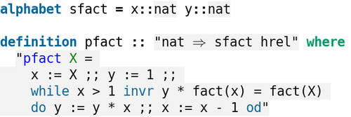
Figure 7: Factorial Program in Isabelle/UTP

5.2 Operational Semantics

Operational semantics are commonly assigned to a programming language by means of an inductive set of transition rules [63]. UTP [57, chapter 10], however, takes a different approach. As usual it characterises a small-step operational semantics for imperative programs using a step relation, $(s,P)\to(t,Q)$, meaning that program $P$, when started in state $s$, can transition to program $Q$, with state $t$. However, instead of characterising this relation using an inductive set, it gives a denotational semantics to the transition relation, and then proves transition rules as theorems. This has the benefit that linking operational and axiomatic semantics is straightforward.

Here, we adopt a similar idea to describe a reduction semantics for relational programs, and use it to perform symbolic execution, following the pattern given by Gordon and Collavizza [47]. We begin by describing the execution of a program $P$ started in a state context $\Gamma$.

Definition 5.2 (Program Evaluation).

$\llparenthesis\Gamma,P\rrparenthesis\,\triangleq\,\left\langle\Gamma\right\rangle\mathrel{\hbox{\rm;}}P$ where $P:[\mathcal{S}]\textit{{hrel}}$ and $\Gamma:\mathcal{S}\to\mathcal{S}$.

The meaning of $\llparenthesis\Gamma,P\rrparenthesis$ is that program $P$ is executed in the variable context $\Gamma$, which gives assignments to a selection of variables in $\mathcal{S}$, for example $[x\mapsto_{\tiny{\textnormal{{s}}}}5,y\mapsto_{\tiny{\textnormal{{s}}}}\textit{{true}}]$. The expression $\llparenthesis\Gamma,{\hbox{{I \kern-8.5ptI}}}\rrparenthesis$ denotes a program that has terminated in state $\Gamma$. The definition above of this operator is very simple, because of our encoding of variable contexts as substitutions: we apply $\Gamma$ as an assignment, and compose this with the program $P$. Using this definition we can prove a set of reduction theorems.

Theorem 5.3 (Operational Reduction Rules).

—$P$   $\llparenthesis\Gamma,P\mathrel{\hbox{\rm;}}Q\rrparenthesis\rightarrow\llparenthesis\Gamma,P\rrparenthesis\mathrel{\hbox{\rm;}}Q$

—$P$   $\llparenthesis\Gamma,\left\langle\sigma\right\rangle\rrparenthesis\rightarrow\llparenthesis\sigma\mathrel{\circ}\Gamma,{\hbox{{I \kern-8.5ptI}}}\,\rrparenthesis$

$(\Gamma\mathop{\dagger}b)\rightarrow\textit{{true}}$   $\llparenthesis\Gamma,P\mathop{\hbox{\raisebox{0.0pt}{$\leftslice$}}}b\mathop{\hbox{\raisebox{0.0pt}{$\rightslice$}}}Q\rrparenthesis\rightarrow\llparenthesis\Gamma,P\rrparenthesis$	$(\Gamma\mathop{\dagger}b)\rightarrow\textit{{false}}$   $\llparenthesis\Gamma,P\mathop{\hbox{\raisebox{0.0pt}{$\leftslice$}}}b\mathop{\hbox{\raisebox{0.0pt}{$\rightslice$}}}Q\rrparenthesis\rightarrow\llparenthesis\Gamma,Q\rrparenthesis$
$(\Gamma\mathop{\dagger}b)\rightarrow\textit{{true}}$   $\llparenthesis\Gamma,b\oast P\rrparenthesis\rightarrow\llparenthesis\Gamma,P\mathrel{\hbox{\rm;}}(b\oast P)\rrparenthesis$	$(\Gamma\mathop{\dagger}b)\rightarrow\textit{{false}}$   $\llparenthesis\Gamma,b\oast P\rrparenthesis\rightarrow\llparenthesis\Gamma,{\hbox{{I \kern-8.5ptI}}}\,\rrparenthesis$

The arrow $P\rightarrow Q$ actually denotes an equality predicate ($P=Q$); we use the arrow notation to aid in comprehension, and to emphasise the left-to-right nature of semantic evaluations. The first two rules on the top line handle sequential composition. The first pushes an evaluation into the first argument of a composition $P\mathrel{\hbox{\rm;}}Q$. The second rule states that when the first argument of a sequential composition has terminated (I I), execution moves on to the second argument ($P$). The third rule handles assignments, creating a new context by precomposing the assignment $\sigma$ with the current context.

The second and third lines deal with conditional and while-loop iteration, respectively. In all these rules, the context $\Gamma$ is applied to the condition $b$ as a substitution. If the result is true, the conditional chooses the first branch $P$, and the while loop makes a copy of the loop body. If the result is false, the conditional chooses the second branch $Q$, and the while loop terminates.

Using these theorems, we can perform symbolic execution of programs in Isabelle/UTP. To achieve this we load the Isabelle simplifier with the equations of both Theorem 5.3 and Lemma 4.16, the latter of which allows us to apply substitutions. We also utilise the pointwise-lifted semantics given in §4.1 to evaluate expressions using the builtin HOL functional definitions and simplification laws.

In addition, we need the equations of Lemma 4.13 to evaluate and normalise substitutions. However, Law SB4, which allows reordering of subsitution maplets, is symmetric and therefore cannot be directly used as it would cause the simplifier to loop. The issue is that lenses do not apriori have a total order that can be used to reorder them. Nevertheless, Law SB4 is important to enable a canonical representation of concrete substitutions. Consequently, we extend the simplifier with a “simproc” [64], a specialised meta-logical simplification procedure that sorts substitution maplets lexicographically using the syntactic lens names. Thus, during symbolic evaluation the variable context will always order the variables lexicographically.

Applying the Isabelle simplifier with these laws, we can symbolically execute programs. Below, we give an example execution of the factorial program from Example 5.1. We do this by using the simplifier to evaluate the term $\llparenthesis id,pfact(4)\rrparenthesis$, where $id$ encodes an arbitrary initial assignment for all the variables.

Example 5.4 (Factorial Symbolic Execution).

$$\llparenthesis id,pfact(4)\rrparenthesis$$

$$=\,\, \llparenthesis id,x:=4\mathrel{\hbox{\rm;}}y:=1\mathrel{\hbox{\rm;}}(x>1)\oast(y:=y*x\mathrel{\hbox{\rm;}}x:=x-1)\rrparenthesis$$

$$=\,\, \llparenthesis[x\mapsto_{\tiny{\textnormal{{s}}}}4],y:=1\mathrel{\hbox{\rm;}}(x>1)\oast(y:=y*x\mathrel{\hbox{\rm;}}x:=x-1)\rrparenthesis$$

$$=\,\, \llparenthesis[x\mapsto_{\tiny{\textnormal{{s}}}}4,y\mapsto_{\tiny{\textnormal{{s}}}}1],(x>1)\oast(y:=y*x\mathrel{\hbox{\rm;}}x:=x-1)\rrparenthesis$$

$$=\,\, \llparenthesis[x\mapsto_{\tiny{\textnormal{{s}}}}4,y\mapsto_{\tiny{\textnormal{{s}}}}1],(y:=y*x\mathrel{\hbox{\rm;}}x:=x-1)\mathrel{\hbox{\rm;}}(x>1)\oast(y:=y*x\mathrel{\hbox{\rm;}}x:=x-1)\rrparenthesis$$

$$=\,\, \llparenthesis[x\mapsto_{\tiny{\textnormal{{s}}}}4,y\mapsto_{\tiny{\textnormal{{s}}}}4],x:=x-1\mathrel{\hbox{\rm;}}(x>1)\oast(y:=y*x\mathrel{\hbox{\rm;}}x:=x-1)\rrparenthesis$$

$$=\,\, \llparenthesis[x\mapsto_{\tiny{\textnormal{{s}}}}3,y\mapsto_{\tiny{\textnormal{{s}}}}4],(x>1)\oast(y:=y*x\mathrel{\hbox{\rm;}}x:=x-1)\rrparenthesis$$

$$=\,\, \llparenthesis[x\mapsto_{\tiny{\textnormal{{s}}}}2,y\mapsto_{\tiny{\textnormal{{s}}}}12],(x>1)\oast(y:=y*x\mathrel{\hbox{\rm;}}x:=x-1)\rrparenthesis$$

$$=\,\, \llparenthesis[x\mapsto_{\tiny{\textnormal{{s}}}}1,y\mapsto_{\tiny{\textnormal{{s}}}}24],(x>1)\oast(y:=y*x\mathrel{\hbox{\rm;}}x:=x-1)\rrparenthesis$$

$$=\,\, \llparenthesis[x\mapsto_{\tiny{\textnormal{{s}}}}1,y\mapsto_{\tiny{\textnormal{{s}}}}24],{\hbox{{I \kern-8.5ptI}}}\,\rrparenthesis$$

In this case, the program terminates in final state $[x\mapsto_{\tiny{\textnormal{{s}}}}1,y\mapsto_{\tiny{\textnormal{{s}}}}24]$, but in the case of a non-terminating program the simplifier will loop. Such a symbolic execution engine is a useful tool for simulation of programs.

Next, we show how we can mechanise the rules of Hoare logic and apply them to verification.

5.3 Hoare Logic

A Hoare triple $\hbox{\large${\{}$}b\hbox{\large${\}}$}\,P\,\hbox{\large${\{}$}c\hbox{\large${\}}$}$ is an assertion that, if program $P$ is started in a state satisfying predicate $b$, then all final states satisfy predicate $c$. The UTP book [57, chapter 2] shows how this assertion can be encoded using a refinement statement. Their definition is mechanised in Isabelle/UTP as given below.

Definition 5.5 (Hoare Triple).

$\hbox{\large${\{}$}b\hbox{\large${\}}$}\,P\,\hbox{\large${\{}$}c\hbox{\large${\}}$}\triangleq((b^{\mbox{\!\! $\blacktriangleleft$}}\mathrel{\Rightarrow}c^{\mbox{\!\! $\blacktriangleright$}})\mathrel{\sqsubseteq}P)$

This states that the Hoare triple is valid when $P$ is a refinement of the specification $b^{\mbox{\!\! $\blacktriangleleft$}}\mathrel{\Rightarrow}c^{\mbox{\!\! $\blacktriangleright$}}$. The specification states that when $b$ is satisfied initially, then $c$ is satisfied finally. This is a statement of partial correctness since $P$ could satisfy this condition by not terminating, for example if $P=\hbox{{{{false}}}}$, since $Q\mathrel{\sqsubseteq}\hbox{{{{false}}}}$ for any $Q$. Definition 5.5 is equivalent to the standard definition for partial correctness [46] illustrated in Section 2.3:

Theorem 5.6.

$\hbox{\large${\{}$}b\hbox{\large${\}}$}\,P\,\hbox{\large${\{}$}c\hbox{\large${\}}$}\mathrel{\Leftrightarrow}\left(\mathop{\mathstrut{\forall}}\nolimits(s,s^{\prime})@b(s)\mathrel{\wedge}P(s,s^{\prime})\mathrel{\Rightarrow}c(s^{\prime})\right)$

An equivalent characterisation is given in terms of our reduction relation below.

Theorem 5.7.

If $\hbox{\large${\{}$}b\hbox{\large${\}}$}\,P\,\hbox{\large${\{}$}c\hbox{\large${\}}$}$ then $\mathop{\mathstrut{\forall}}\nolimits(\Gamma_{1},\Gamma_{2})@[(\Gamma_{1}\mathop{\dagger}b)\mathrel{\wedge}\llparenthesis\Gamma_{1},P\rrparenthesis\rightarrow\llparenthesis\Gamma_{2},{\hbox{{I \kern-8.5ptI}}}\,\rrparenthesis\mathrel{\Rightarrow}(\Gamma_{2}\mathop{\dagger}c)]$

This is an example of a UTP linking theorem [57] that relates two semantic presentations, in this case how the Hoare triple is related to the operational semantics. The satisfaction of $\hbox{\large${\{}$}b\hbox{\large${\}}$}\,P\,\hbox{\large${\{}$}c\hbox{\large${\}}$}$ implies that, for any initial state assignment $\Gamma_{1}$ satisfying precondition $b$, if $P$ terminates with final state assignment $\Gamma_{2}$, then $\Gamma_{2}$ satisfies $c$. Thus we have formally related the operational and axiomatic semantics for relational programs. From Definition 5.5 we can also prove, as theorems, the following Hoare calculus laws:

Theorem 5.8 (Hoare Calculus Laws).

$\hbox{\large${\{}$}b\hbox{\large${\}}$}\,P\,\hbox{\large${\{}$}c\hbox{\large${\}}$}$$[p\mathrel{\Rightarrow}\sigma\mathop{\dagger}q]$        $\hbox{\large${\{}$}p\hbox{\large${\}}$}\,\left\langle\sigma\right\rangle\,\hbox{\large${\{}$}q\hbox{\large${\}}$}$

$\hbox{\large${\{}$}p\mathrel{\wedge}b\hbox{\large${\}}$}\,S\,\hbox{\large${\{}$}p\hbox{\large${\}}$}$   $\hbox{\large${\{}$}p\hbox{\large${\}}$}\,b\oast P\,\hbox{\large${\{}$}\neg b\mathrel{\wedge}p\hbox{\large${\}}$}$

The majority of these laws are standard [54]. However, the formulation of the assignment law is more general than the standard law, $\hbox{\large${\{}$}p[e/x]\hbox{\large${\}}$}\,x:=e\,\hbox{\large${\{}$}p\hbox{\large${\}}$}$. It avoids the aliasing problem of classical Hoare logic since substitution depends on semantic independence of lenses, rather than syntactic inequality of variable names. We can model aliased names by giving a lens two (meta-logical) names in Isabelle, $x$ and $y$. We can also consider the situation when $x$ and $y$ are different constructions and yet not independent, such as $hp$ and $hp[0]$, from Example 2.3. We illustrate this with the following example.

Example 5.9 (Aliasing).

We consider the triple $\hbox{\large${\{}$}y=3\hbox{\large${\}}$}\,x:=2\,\hbox{\large${\{}$}y=3\hbox{\large${\}}$}$. If we attempt its proof using the rules above, and the substitution laws (Lemma 4.16), the result is the predicate $(y=3)\mathrel{\Rightarrow}(y[2/x]=3)$. If $x$ and $y$ are identical ($x=y$) then this reduces to $(y=3)\mathrel{\Rightarrow}\textit{{false}}$, which is not provable. If $x\neq y$, and yet either $x\approx y$, $x\preceq y$, or $y\preceq x$, then the conjecture is also not provable; indeed we can use nitpick [13, 12] to find a counterexample. If, however, $x\mathop{\,\bowtie\,}y$, then we obtain $(y=3)\mathrel{\Rightarrow}(y=3)$, which is true. ∎

Similarly, from Definition 5.5 we can also represent derived laws, like the forward assignment law, by making use of unrestriction.

Lemma 5.10.

$\hbox{\large${\{}$}p\hbox{\large${\}}$}\,x:=e\,\hbox{\large${\{}$}x=e\mathrel{\wedge}p\hbox{\large${\}}$}\quad\text{if }x\mathop{\sharp}e,x\mathop{\sharp}p$

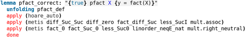
Figure 8: Verification of Factorial Algorithm

We can use these laws to automatically verify our factorial program, following the pattern of previous works [2, 63, 3], though using our lens-based Hoare logic laws. We require, as usual, that the program is annotated with loop invariants. This is shown in Figure 7, with loop invariant $y*x!=X!$, which is syntactic sugar to help the proof strategy [3]. The proof strategy, implemented in the Isabelle/UTP tactic hoare-auto, executes the following steps:

1. Combine all composed assignments using Corollary 4.24.

2. Apply the Hoare logic laws of Theorem 5.8 as deduction rules.

3. Perform any substitutions in the resulting predicates using Lemma 4.13 and Lemma 4.16.

4. Apply the rel-auto tactic of §4.1 to each resulting predicate.

The result is a set of HOL predicates that characterise the verification conditions for the program. We exemplify this with the factorial program below.

Example 5.11.

$\hbox{\large${\{}$}\textit{{true}}\hbox{\large${\}}$}\,pfact(\textit{{X}})\,\hbox{\large${\{}$}y=X!\hbox{\large${\}}$}$

Proof.

Application of hoare-auto yields the following verification conditions:

1. $\textit{{x}}>1\mathrel{\wedge}\textit{{y}}*\textit{{x}}!=X!\mathrel{\Rightarrow}\textit{{y}}*\textit{{x}}*(\textit{{x}}-1)!=\textit{{X}}!$

2. $\textit{{x}}\leq 1\mathrel{\wedge}\textit{{y}}*\textit{{x}}!=X!\mathrel{\Rightarrow}\textit{{y}}=\textit{{X}}!$

In this case, both proof obligations can be discharged using sledgehammer [12]. This is illustrated in Figure 8, with calls to metis for each proof obligation. ∎

As a further example we consider a program for the find and replace functionality in a text editor.

Example 5.12 (Find and Replace).

$$\begin{array}[]{l}\hbox{{{{function}}}}\,\textit{find-replace}(arr:[string]array,len:nat,mtc:string,rpl:string):nat\triangleq\\ \quad\hbox{{{{var}}}}\,i,occ:nat@\\ \quad i:=0\mathrel{\hbox{\rm;}}occ:=0\mathrel{\hbox{\rm;}}\\ \quad\hbox{{{{while}}}}\,i<len\,\hbox{{{{do}}}}\\ \qquad\hbox{{{{if}}}}\,arr[i]=mtc\,\hbox{{{{then}}}}\,arr[i]:=rpl\mathrel{\hbox{\rm;}}occ:=occ+1\,\hbox{{{{else}}}}\,arr[i]:=arr[i]\hbox{{{{fi}}}}\mathrel{\hbox{\rm;}}\\ \qquad i:=i+1\\ \quad\hbox{{{{od}}}}\mathrel{\hbox{\rm;}}\\ \quad\hbox{{{{return}}}}\,occ\end{array}$$

In this program, we have an array of strings that represents a sequence of words in a text buffer, and we wish to replace every occurence of a particular string, $mtc$, with another string $rpl$. The specified function takes four parameters: an array of strings, $arr$, the length of the array $len$, and the two strings $mtc$ and $rpl$. It returns the number of occurences for which it has made a replacement.

We first create local variables $i$ and $occ$, using the var construct, and initialise them, for iterating over the list and recording occurrences. We then have a while loop that iterates over the length of the array. At each step, if the $i$th element of the array equals $mtc$, then this element is replaced with $rpl$, and the number of occurences is incremented. Otherwise, the element of the array is left unchanged. Finally, $i$ is incremented and the loop continues. Once the loop exits, the value of $occ$ is returned. Variables $occ$ and $i$ are modelled in Isabelle/UTP using record lenses, and the array $arr$ using a total function lens.

The algorithm is mechanised in Isabelle/UTP as shown in Figure 9. We first create the state space $ss$ with variables $arr$, $occ$, and $i$. We represent the variables $len$, $mtc$, and $rpl$ as logical variables, since they are not changed by the algorithm. Moreover, we include an explicit parameter $A$ that represents the initial state of the array. This is need to represent the invariant annotations, which we explain below.

There are at least two desirable properties for this program, both of which are postconditions: (1) $arr$ should have all occurrences of $mtc$ replaced with $rpl$; and (2) the value of $occ$ returned should be number of occurrences in $arr$ initially. The first can be represented by the following triple:

$$\hbox{\large${\{}$}arr=\textit{{A}}\hbox{\large${\}}$}\,\textit{find-replace}(arr,len,mtc,rpl)\,\hbox{\large${\{}$}\mathop{\mathstrut{\forall}}\nolimits i<len@\textit{{A}}[i]=(mtc\mathop{\hbox{\raisebox{0.0pt}{$\leftslice$}}}arr[i]=rpl\mathop{\hbox{\raisebox{0.0pt}{$\rightslice$}}}\textit{{A}}[i])\hbox{\large${\}}$}$$

This states that if the array is initially A, then following execution of find-replace, for every index $i$ in A that has $mtc$, the array contains $rpl$, and all other elements remain the same. This can be proved using the invariants shown in Figure 9. It has two parts corresponding to properties (1) and (2). The first invariant states that at the $i$th iteration, $arr$ is identical to $A$, except that every instance of $mtc$ up to index $i$ is replaced with $rpl$. The second invariant states that the number of occurrences is equal to the number of instances of $mtc$ filtered out of the function before index $i$. The third invariant is that $i\leq len$. With these three invariants, we can verify the two properties; this is illustrated in Figure 10.

Thus we have shown how Isabelle/UTP can be applied to practical verification of relational programs, which can contain complex state space structures afforded by lenses. We can unify different variants of assignment, such as to multiple variables and collections, using the generalised assignment law. Moreover, the verification infrastructure is semantic and thus efficient in nature, without the need for deep syntax, and yet can utilise meta-logical concepts like substitution and unrestriction, which are not present in other shallow embeddings.

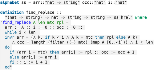
Figure 9: Find and Replace in Isabelle/UTP

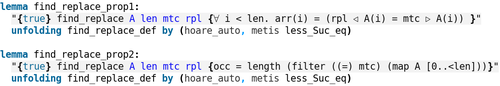
Figure 10: Find and Replace verified in Isabelle/UTP

In the next section we consider the mechanisation of Morgan’s refinement calculus.

5.4 Refinement Calculus

In this section, we show how lenses can support a Morgan-style refinement calculus [61], extending our previous results on frames in UTP [35]. The refinement calculus is a technique for stepwise development of programs, by refining abstract specifications in increasingly concrete programs. The specification statement, $w{:}[pre,post]$, is a contract asserting that (1) only the variables in $w$ may change, and (2) the postcondition ($post$) should be established when the precondition ($pre$) holds. We use lenses and our relational program model to mechanise a partial correctness specification statement, and prove several laws relating to frames. Ordinarily, Morgan’s calculus specified total correctness, but here we focus on the laws relating to frames, rather than termination of programs. A total correctness calculus can be obtained straightforwardly by combining our results here and in Section 6 with the UTP theory of designs [57, 20].

For this, we first define a notion of equivalence modulo a lens that is needed to characterise frames.

Definition 5.13 (Observation Equivalence).

We assume $s_{1},s_{2}:\mathcal{S}$ and $X:\mathcal{V}\Longrightarrow\mathcal{S}$, and define:

$$s_{1}\simeq_{X}s_{2}\triangleq(s_{1}=\textit{{put}}_{X}\,s_{2}\,(\textit{{get}}_{X}\,s_{1}))$$

This operator states that two states $s_{1}$ and $s_{2}$ are the same everywhere outside of the region described by $X$. For example, if we have three variables $x,y,z:{\mathbb{Z}}$, then we can show that

$$[x\mapsto 1,y\mapsto 2,z\mapsto 3]\simeq_{x}[x\mapsto 2,y\mapsto 2,z\mapsto 3]$$

since the two states differ only in the value of $x$. Lenses can represent sets of variables, using $+$, and so we can group several independent variables in a frame, as the following equivalences illustrate:

Lemma 5.14.

Assume $s_{1},s_{2}:\mathcal{S}$ then the following identities hold:

$$(s_{1}\simeq_{\mathbf{1}_{\mathcal{S}}}s_{2})=\textit{{true}}\text{\penalty 10000\ and\penalty 10000\ }(s_{1}\simeq_{\mathbf{0}_{\mathcal{S}}}s_{2})=(s_{1}=s_{2})$$

This theorem demonstrates the intuition that $\mathbf{1}$ and $\mathbf{0}$ characterise the entirety and none of the state space, respectively. The state space outside of $\mathbf{1}$ is empty, and outside of $\mathbf{0}$ is the whole state. We can also show that $\simeq_{X}$ is an equivalence relation.

Lemma 5.15.

If $X$ is a total lens then $\simeq_{X}$ is an equivalence relation on states.

We now use observation equivalence to define the specification statement.

Definition 5.16 (Specification Statement).

$$w{:}[pre,post]\triangleq((pre^{\mbox{\!\! $\blacktriangleleft$}}\mathrel{\Rightarrow}post^{\mbox{\!\! $\blacktriangleright$}})\mathrel{\wedge}\hbox{{{{v}}}}^{\mbox{\!\! $\blacktriangleleft$}}\simeq_{w}\hbox{{{{v}}}}^{\mbox{\!\! $\blacktriangleright$}})$$

A specification statement states that the precondition implies the postcondition, and in addition the initial state is the same as the final state, modulo $w$. The semantics is similar to the partial correctness Hoare triple in Definition 5.5, except that it only includes the specification. Indeed, we can prove the following well-known correspondence [57, 45].

Theorem 5.17.

$\hbox{\large${\{}$}pre\hbox{\large${\}}$}\,P\,\hbox{\large${\{}$}post\hbox{\large${\}}$}\mathrel{\Leftrightarrow}(\hbox{{{{v}}}}{:}[pre,post]\mathrel{\sqsubseteq}P)$

A Hoare triple can be re-expressed as a specification statement refinement. The standard triple does not include a frame, and consequently all variables are permitted to change, indicated by the frame being v (i.e. $\mathbf{1}$). Moreover, from Definition 5.16 we can derive many of the refinement calculus laws [61] as theorems.

Theorem 5.18 (Refinement Calculus).

If $x$ and $w$ are total lenses, then the following laws hold:

$$w{:}[pre,post] \mathrel{\sqsubseteq}w{:}[pre,post^{\prime}] \text{if }post^{\prime}\mathrel{\Rightarrow}post$$ (1)

$$w{:}[pre,post] \mathrel{\sqsubseteq}w{:}[pre^{\prime},post] \text{if }pre\mathrel{\Rightarrow}pre^{\prime}$$ (2)

$$x,w{:}[pre,post] \mathrel{\sqsubseteq}w{:}[pre,post] \text{if }x\mathop{\,\bowtie\,}w$$ (3)

$$w{:}[pre,post] \mathrel{\sqsubseteq}{\hbox{{I \kern-8.5ptI}}} \text{if }pre\mathrel{\Rightarrow}post$$ (4)

$$w{:}[pre,post] \mathrel{\sqsubseteq}x:=e \text{if }x\preceq w,pre\mathrel{\Rightarrow}post[e/x]$$ (5)

$$(w:=e) =w{:}[\textit{{true}},w=e] \text{if }w\mathop{\sharp}e$$ (6)

$$w{:}[pre,post] \mathrel{\sqsubseteq}w{:}[pre,mid]\mathrel{\hbox{\rm;}}w{:}[mid,post]$$ (7)

$$w{:}[pre,post] \mathrel{\sqsubseteq}w{:}[b\mathrel{\wedge}pre,post]\mathop{\hbox{\raisebox{0.0pt}{$\leftslice$}}}b\mathop{\hbox{\raisebox{0.0pt}{$\rightslice$}}}w{:}[(\neg b)\mathrel{\wedge}pre,post]$$ (8)

These laws use the lens operators as side conditions. Laws (1) and (2) allows strengthening and weakening of a post- and precondition, respectively. Law (3) shows that a variable can be removed from a frame in a refinement, because this effectively adds $x^{\mbox{\!\! $\blacktriangleright$}}=x^{\mbox{\!\! $\blacktriangleleft$}}$ as a conjunct. Laws (4) and (5) show the circumstances under which a specification may be refined to a skip (I I) or assignment ($x:=e$). For the latter, $x$ must be in the frame $w$, represented by $x\preceq w$. Law (6) shows that an assignment $w:=e$ can be written as a specification statement when $e$ does not depend on $w$. Law (7) shows how a specification can be divided into two sequential specifications by inserting a midpoint condition. Finally, (8) shows how a conditional can be introduced, by conjoining the precondition with predicate $b$.

These results illustrate how lenses support modelling of frames. The theorems can be applied to derivation of algorithms by stepwise refinement in Isabelle/UTP. We have therefore shown in this section how our lens-based semantic foundation allows us to support a selection of verification calculi and linking theorems between them. In the next section we consider mechanisation of UTP theories.

6 Mechanising UTP Theories

In this section we apply Isabelle/UTP to the mechanisation of UTP theories. The relational program model in §4 is powerful, but not without limitations. It is well known, for instance, that simple relational programs, which capture only the possible initial and final values of program variables, cannot adequately differentiate terminating and non-terminating behaviour [21]. Furthermore, several programming paradigms, such as real-time, concurrency, and object orientation, require a richer semantic model with more observable information [21, 72, 74, 33].

This semantic enrichment can be facilitated by UTP theories. Semantic information is expressed by adding special observational variables, which encode quantities of a program or model, and invariants that restrict their domain, called healthiness conditions. The observational variables can be used to define specialised operators for a particular computational paradigm, such as a delay or deadline operator for a real-time language. For example, a clock variable, $clock:{\mathbb{N}}$ can be added to record to passage of time, or a trace variable $tr:[\textit{Event}]list$ can be added to record events [21]. The healthiness conditions allow us to impose well-formedness invariants over these observational variables, and allow us to prove algebraic theorems that characterise the healthy elements. As usual, healthiness conditions are represented as idempotent predicate transformers, that is, functions on relations over the observational variables. The pay-off here is that general properties of elements of the UTP theory can often be reduced to properties of the healthiness conditions [57, 36].

We characterise UTP theories in Isabelle/UTP as follows.

Definition 6.1.

An Isabelle/UTP theory is a pair ($\mathcal{S}$, $\mathcal{H}$), where $\mathcal{S}$ is an observation (i.e. state) space, $\mathcal{H}:[\mathcal{S}]\textit{{hrel}}\to[\mathcal{S}]\textit{{hrel}}$ is a healthiness condition, and $\mathcal{H}$ is idempotent: $\mathcal{H}\mathrel{\circ}\mathcal{H}=\mathcal{H}$.

We mechanise this algebraic structure in Isabelle using locales [8]. $\mathcal{S}$ characterises the observations that can be made of the model. An observation space can be constructed using the alphabet command (§3.6), in which case it defines a set of lenses, $x_{1}\cdots x_{n}$, which provide the observational variables. The healthiness conditions are encoded as total endofunctions on homogeneous relations parameterised by $\mathcal{S}$. If a theory has multiple healthiness conditions, then these can be composed function-wise. The simplest UTP theory is the relational theory, $Rel_{\alpha}\triangleq(\alpha,\mathop{\mathstrut{\lambda}}\nolimits X@X)$. Any type is an instance of $\alpha$, and any relation is a fixed-point of $\mathop{\mathstrut{\lambda}}\nolimits X@X$.

We say that a relation $P:[\mathcal{S}]\textit{{hrel}}$ is $\mathcal{H}$-healthy, written $P\mathop{\,\textit{is}\,}\mathcal{H}$, when $P$ is a fixed-point of $\mathcal{H}$: $\mathcal{H}(P)=P$. Moreover, we characterise the healthy elements of a theory by the set $\llbracket\mathcal{H}\rrbracket_{\mbox{\tiny{{H}}}}\triangleq\{P|P\mathop{\,\textit{is}\,}\mathcal{H}\}$. Idempotence of $\mathcal{H}$ guarantees the existence of at least one fixed point. This ensures that the UTP theory is non-empty since, for any relation $P$, $\mathcal{H}(P)\in\llbracket\mathcal{H}\rrbracket_{\mbox{\tiny{{H}}}}$ since $\mathcal{H}(\mathcal{H}(P))=\mathcal{H}(P)$. To illustrate, we formalise the UTP theory for timed relational programs introduced in §2.1.

Example 6.2 (Timed Relations).

The parametric observation space $[S]\textit{{rt}}\,\triangleq\,\left[clock:\mathbb{N},st:S\right]$ has lenses $clock:\mathbb{N}$, which denotes the passage of time, and $st:S$, which denotes the user state. Healthiness function

$$\hbox{{{{HT}}}}(P)\triangleq(clock^{\mbox{\!\! $\blacktriangleleft$}}\leq clock^{\mbox{\!\! $\blacktriangleright$}}\mathrel{\wedge}P)$$

ensures that time advances. HT is clearly idempotent, since conjunction is idempotent. We define the following operator for introducing a delay for timed relations:

wait $$:\mathbb{N}\to[[S]\textit{{rt}}]\textit{{hrel}}$$

$$\hbox{{{{wait}}}}(n) \triangleq(clock^{\mbox{\!\! $\blacktriangleright$}}=clock^{\mbox{\!\! $\blacktriangleleft$}}+n\mathrel{\wedge}st^{\mbox{\!\! $\blacktriangleright$}}=st^{\mbox{\!\! $\blacktriangleleft$}})$$

Here, $clock$ is advanced by $n$, and the state is unchanged. We can prove that $\hbox{{{{wait}}}}(n)$ is HT-healthy, since it advances time. Conversely, the predicate $clock^{\mbox{\!\! $\blacktriangleright$}}=clock^{\mbox{\!\! $\blacktriangleleft$}}-1$ is not healthy, since it tries to reverse time. The mechanisation of the theory in Isabelle/UTP is shown in Figure 11. ∎

As in previous work [26, 79], our theories form “families”: they characterise relations on several observation spaces, since the observation type is potentially polymorphic, and thus extensible with additional variables. For example, our theory in Example 6.2 is parametric in $S$. We can characterise a subtheory relation between UTP theories.

Definition 6.3.

$([\bm{\beta}]\mathcal{T}_{2},\mathcal{H}_{2})$ is a subtheory of $(\mathcal{S}_{1},\mathcal{H}_{1})$ when $[\bm{\beta}]\mathcal{T}_{2}$ specialises $\mathcal{S}_{1}$, and $\llbracket\mathcal{H}_{2}\rrbracket_{\mbox{\tiny{{H}}}}\subseteq\llbracket\mathcal{H}_{1}\rrbracket_{\mbox{\tiny{{H}}}}$.

Subtheories allow us to arrange theories in a hierarchy with descendants that specialise the observation space with additional variables and constraints.

UTP theories also include a signature: a set of operators that construct healthy elements of the theory. We say that an operator

$$F:[\mathcal{S}]\textit{{hrel}}^{\,n}\to[\mathcal{S}]\textit{{hrel}}$$

in $n$ parameters, is in the signature if $\llbracket\mathcal{H}\rrbracket_{\mbox{\tiny{{H}}}}$ is closed under $F$. Formally, we require that:

$$\mathop{\mathstrut{\forall}}\nolimits P_{1},\cdots,P_{n}\,@\,P_{1}\mathop{\,\textit{is}\,}\mathcal{H}\mathrel{\wedge}\cdots\mathrel{\wedge}P_{n}\mathop{\,\textit{is}\,}\mathcal{H}\,\,\Longrightarrow\,\,F(P_{1},\cdots,P_{n})\mathop{\,\textit{is}\,}\mathcal{H}$$

The function $F$ can either denote a new operator defined on $\mathcal{S}$, or an existing operator defined over a parent observation space. For example, nondeterministic choice $P\sqcap Q$ and sequential composition $P\mathrel{\hbox{\rm;}}Q$ often inhabit the signature of several theories, since they are typed by arbitrary relations and so can be instantiated by any observation space. This also means that the corresponding algebraic laws for a parent operator $F$ can be directly applied to elements of a new subtheory. For example, sequential composition is always associative, since every theory is a subtheory of $Rel_{\alpha}$.

We exemplify this by giving the signature of our theory of timed relations.

Lemma 6.4.

$\llbracket\hbox{{{{HT}}}}\rrbracket_{\mbox{\tiny{{H}}}}$ is closed under the following relational operators: I I, $\mathrel{\hbox{\rm;}}$, $\mathop{\hbox{\raisebox{0.0pt}{$\leftslice$}}}b\mathop{\hbox{\raisebox{0.0pt}{$\rightslice$}}}$, and $x:=v$ when $x\mathop{\,\bowtie\,}clock$, and so these are also within the theory signature, as demonstrated by the laws below:

—$P$   ${\hbox{{I \kern-8.5ptI}}}\mathop{\,\textit{is}\,}\hbox{{{{HT}}}}$

—$P$   $\hbox{{{{wait}}}}(n)\mathop{\,\textit{is}\,}\hbox{{{{HT}}}}$

Once the signature operators have been established, the final step is to prove the characteristic algebraic theorems for them. These laws effectively provide an algebraic semantics for the UTP theory, and can be used to aid in the construction of program verification tools. There are three ways to obtain such theorems in Isabelle/UTP. Firstly, we can inherit them from a parent theory by utilising Definition 6.3. Secondly, we can import them from an algebraic structure by proving the algebra’s axioms. Thirdly, we can prove them manually using Isabelle/UTP’s proof tactics.

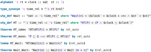
Figure 11: Timed Relations in Isabelle/UTP

We exemplify the third approach for the new delay operator, using our rel-auto proof tactic (§4.1).

Theorem 6.5 (Delay Laws).

$$\hbox{{{{wait}}}}(0) \penalty 10000\ =\,{\hbox{{I \kern-8.5ptI}}}$$

$$\hbox{{{{wait}}}}(m)\mathrel{\hbox{\rm;}}\hbox{{{{wait}}}}(n) \penalty 10000\ =\,\hbox{{{{wait}}}}(m+n)$$

$$\hbox{{{{wait}}}}(m)\mathrel{\hbox{\rm;}}(P\mathop{\hbox{\raisebox{0.0pt}{$\leftslice$}}}b\mathop{\hbox{\raisebox{0.0pt}{$\rightslice$}}}Q) \penalty 10000\ =\,(\hbox{{{{wait}}}}(m)\mathrel{\hbox{\rm;}}P)\mathop{\hbox{\raisebox{0.0pt}{$\leftslice$}}}b\mathop{\hbox{\raisebox{0.0pt}{$\rightslice$}}}(\hbox{{{{wait}}}}(m)\mathrel{\hbox{\rm;}}Q) \text{if }clock\mathop{\sharp}b$$

$$\hbox{{{{wait}}}}(m)\mathrel{\hbox{\rm;}}x:=v \penalty 10000\ =\,x:=v\mathrel{\hbox{\rm;}}\hbox{{{{wait}}}}(m) \text{if }clock\mathop{\sharp}v,x\mathop{\,\bowtie\,}clock$$

Waiting for a zero length duration is simply a skip operation (I I), sequential composition of two delays, by $m$ and $n$ time units, is equivalent to a single $m+n$ delay. A delay distributes through a conditional provided that $b$ does not refer to the $clock$ variable. A delay commutes with an assignment ($x:=v$) provided that the delay expression does not depend on $x$ and $v$ does not depend on $clock$.

Algebraic theorems for UTP theories can also be obtained by linking to a variety of mechanised algebraic structures. The HOL-Algebra library [9], for example, characterises the axioms of partial orders, lattices, complete lattices, Galois connections, and the myriad of theorems that can be derived from them. A substantial advantage of the UTP approach is that algebraic theorems can often be reduced to proving properties of the underlying healthiness conditions, which allows us to obtain laws with minimal effort. We exemplify this by restricting ourselves to a particular subclass of continuous UTP theories.

Definition 6.6.

$\mathcal{H}$ is continuous provided that $\mathcal{H}(\bigsqcap_{i\in A}P(i))=\bigsqcap_{i\in A}\mathcal{H}(P(i))$ whenever $A\neq\emptyset$.

In a continuous theory, the healthiness condition distributes through arbitrary non-empty relational infima. A corollary of this definition is that $\mathcal{H}$ is also monotonic: $P\mathrel{\sqsubseteq}Q\mathrel{\Rightarrow}\mathcal{H}(P)\mathrel{\sqsubseteq}\mathcal{H}(Q)$. So, by the Knaster-Tarski theorem, also part of HOL-Algebra, we can show that $\llbracket\mathcal{H}\rrbracket_{\mbox{\tiny{{H}}}}$ forms a complete lattice under refinement $\mathrel{\sqsubseteq}$. This allows us to import theorems for recursive and iterative programs into a UTP theory.

From the induced complete lattice, we obtain the following operators: infimum $\textstyle{\bigsqcap_{\mbox{\tiny$\mathcal{T}$}}}$, supremum $\textstyle{\bigsqcup_{\mbox{\tiny$\mathcal{T}$}}}$, top element $\top_{\mbox{\tiny$\mathcal{T}$}}$, bottom element $\bot_{\mbox{\tiny$\mathcal{T}$}}$, and least fixed-point $\mathop{\mathstrut{\mu}}\nolimits_{\mbox{\tiny$\mathcal{T}$}}$, which are all in the theory’s signature, and for which the usual complete lattice and fixed-point calculus theorems [7] hold. Moreover, in a continuous UTP theory, these operators can be calculated using the equational theorems given below.

Lemma 6.7 (Continuous Theory Properties).

$$\top_{\mbox{\tiny$\mathcal{T}$}} =\mathcal{H}(\hbox{{{{false}}}})$$

$$\bot_{\mbox{\tiny$\mathcal{T}$}} =\mathcal{H}(\hbox{{{{true}}}})$$

$$\textstyle{\bigsqcap_{\mbox{\tiny$\mathcal{T}$}}}\,A =\left(\top_{\mbox{\tiny$\mathcal{T}$}}\mathop{\hbox{\raisebox{0.0pt}{$\leftslice$}}}A=\emptyset\mathop{\hbox{\raisebox{0.0pt}{$\rightslice$}}}\textstyle{\bigsqcap A}\right) \text{if }A\subseteq\llbracket\mathcal{H}\rrbracket_{\mbox{\tiny{{H}}}}$$

$$\mathop{\mathstrut{\mu}}\nolimits_{\mbox{\tiny$\mathcal{T}$}}\,F =\mathop{\mathstrut{\mu}}\nolimits X@F(\mathcal{H}(X)) \text{if }F:\llbracket\mathcal{H}\rrbracket_{\mbox{\tiny{{H}}}}\to\llbracket\mathcal{H}\rrbracket_{\mbox{\tiny{{H}}}}\textnormal{ and }F\textnormal{ is monotonic}$$

These lemmas demonstrate the relationship between the theory operators, and the relational ones defined in §4. The theory top and bottom elements are the relational top and bottom with $\mathcal{H}$ applied. The theory infimum $\textstyle{\bigsqcap_{\mbox{\tiny$\mathcal{T}$}}}\,A$ is $\top_{\mbox{\tiny$\mathcal{T}$}}$ when $A$ is empty, and otherwise the relational infimum. Moreover, the least fixed-point operator can be expressed as the relational least fixed-point by precomposition of $\mathcal{H}$. The utility of these theorems is that we can construct nondeterministic choices and recursive programs using the relational operators $\sqcap$ and $\mathop{\mathstrut{\mu}}\nolimits$, which again allows reuse of their algebraic laws.

We now demonstrate how we can obtain such theorems for timed relations.

Theorem 6.8.

HT is continuous, since conjunction distributes through disjunction ($\bigsqcap$). We therefore obtain a complete lattice, and can calculate the top and bottom element:

$$\top_{\!{\textit{{rt}}}}=\hbox{{{{HT}}}}(\hbox{{{{false}}}})=\hbox{{{{false}}}}\qquad\bot_{{\textit{{rt}}}}=\hbox{{{{HT}}}}(\hbox{{{{true}}}})=(clock\leq clock^{\prime})$$

We also obtain a least fixed-point operator for constructing and reasoning about iteration, $\mathop{\mathstrut{\mu}}\nolimits_{\textit{{rt}}}$, and can use it to denote a timed loop operator: $b\oast_{\textit{{rt}}}P\triangleq(\mathop{\mathstrut{\mu}}\nolimits_{\textit{{rt}}}X@P\mathrel{\hbox{\rm;}}X\mathop{\hbox{\raisebox{0.0pt}{$\leftslice$}}}b\mathop{\hbox{\raisebox{0.0pt}{$\rightslice$}}}{\hbox{{I \kern-8.5ptI}}})$.

From these theorems, we can proceed to define a timed Hoare calculus and proof tactics following the template given in §5. A concrete timed program can be modelled by creating a suitable state space, $vars\,\triangleq\,\left[x_{1}:\tau_{1}\cdots x_{n}:\tau_{n}\right]$, defining the program $P:[[vars]\textit{{rt}}]\textit{{hrel}}$ using the signature operators, and proving that $P\mathop{\,\textit{is}\,}\hbox{{{{HT}}}}$. Finally, the proven Hoare logic deduction rules can be used for program verification.

In this section, we have demonstrated how a UTP theory can be mechanically validated, a set of signature operators verified, and algebraic theorems for these operators proved. Though the example of timed relations is simple, it illustrates the basic concepts that we have used for more complex theories in Isabelle/UTP. Notably, we have applied our approach to the mechanisation of a hierarchy of UTP theories for reactive programs that uses five observational variables and seven healthiness conditions [36]. This UTP theory has been applied to the development of a verification tool for the Circus language [39], which extends our imperative programming language with concurrency and communication [67].

7 Related work

There have been several previous works on application of algebraic semantics to modelling mutation of state. Back and von Wright [6] use two functions $\textsf{val}.x:\mathcal{S}\to\mathcal{V}$ and $\textsf{set}.x:\mathcal{V}\to\mathcal{S}\to\mathcal{S}$, to characterise each variable, together with five axioms that characterise their behaviour.

Definition 7.1 (Back and von Wright’s Variable Axioms [6, 4]).

$$\textsf{val}.x.(\textsf{set}.x.a.\sigma) =a$$ (9)

$$x\neq y\,\mathrel{\Rightarrow}\,\textsf{val}.y.(\textsf{set}.x.a.\sigma) =\textsf{val}.y.\sigma$$ (10)

$$\textsf{set}.x.a\mathrel{\hbox{\rm;}}\textsf{set}.x.b =\textsf{set}.x.b$$ (11)

$$x\neq y\,\mathrel{\Rightarrow}\,\textsf{set}.x.a\mathrel{\hbox{\rm;}}\textsf{set}.y.b =\textsf{set}.y.b\mathrel{\hbox{\rm;}}\textsf{set}.x.a$$ (12)

$$\textsf{set}.x.(\textsf{val}.x.\sigma).\sigma =\sigma$$ (13)

The dot operator ($f.x$) denotes function application in Back and von Wright’s work. From these axioms, and a predicate transformer semantics, they are able to prove the laws of programming [6], including Example 2.1. The lens functions put and get correspond to the variable functions set and val, and have almost the same axioms [30]. Specifically, the axioms of total lenses in Definition 3.5 correspond to Back and von Wright’s axioms (9), (11), and (13) in Definition 7.1. The other two axioms, (12) and (10), are captured by lens independence (Definition 3.8). In fact, Theorem 3.11 demonstrates that only four of Back and von Wright’s variable axioms are necessary [6]; axiom (10) can be proved from the others and so is redundant.

We have based our work on lenses rather than Back and von Wright’s approach, which is also the reason for the different order in the parameters of put [32, 31]. Nevertheless, we effectively use lenses to relax Back and von Wright’s axioms so that we can characterise, not only independence of variables, but also when one variable is “part of” another. Specifically, in Definition 7.1, $x$ and $y$ are individual variables, but with lenses they can equally refer to a set or hierarchical structure. Variable sets are also supported by Back and Preoteasa [4] by lifting these axioms over a list, for instance to support multiple assignment. Our approach has more generality since it allows hierarchy and does not require formalising variable names. Also similar to our work, Back and Preoteasa [4] use their set variable operator to characterise substitution.

J. Foster et al. [31] created lenses as an abstraction for bidirectional programming and solving the view-update problem in database theory [10], which seeks to propagate changes to a computed view table back to the original source table. Fischer et al. [30] give a detailed study of the algebraic laws for get and put, which is the starting point for our work. Foster et al. provide combinators for composing abstract lenses and concrete lenses based on trees [32, 31]. They have been practically applied in the Boomerang language for transformations on textual data structures, such as XML databases. There is also a substantial Haskell library that can be used to develop generic data type transformations. Pickering et al. [69] extend this library to support modular data accessors by introducing various additional combinators, including a form of parallel composition. Our lens sum operator (Definition 3.18) share similarity with the parallel composition operator defined by Pickering et al. [69]. It is different, however, because the latter acts on an explicitly separated state space of the form $A\times B$, whereas lens sum acts on an arbitrary state space.

Variables are also given an algebraic semantics by Dongol et al. [25], through the development of Cylindrical Kleene Algebra, that extends their previous work [3, 45]. The core of their approach is a cylindrification operator, $C_{x}\,R$, that liberates the variable $x$ in relation $R$. Their work contains a comprehensive investigation of the algebraic properties of this operator in an algebraic program model. They apply this algebra to characterise assignment, substitution, and frames. They use a functional model of state [73], and thus need to fix types for both variables and values, as explained in Section 2.4. We hope in the future to apply their algebraic structures and generalise them in the context of lenses, building on our previous results [43, 35]. For comparison, relational cylindrification can effectively be implemented using our lens summation and quantifier operators as $C_{x}\,R\triangleq\mathop{\mathstrut{\exists}}\nolimits\,(x^{\mbox{\!\! $\blacktriangleleft$}}+x^{\mbox{\!\! $\blacktriangleright$}})@R$.

8 Conclusions

In this paper we have given a comprehensive exposition of the foundations of our verification framework, Isabelle/UTP. As we have demonstrated, Isabelle/UTP provides a unified semantic foundation for a variety of computational paradigms and programming languages, with the ability to formulate machine-checked semantic models. These models can then be used in constructing verification tools that harness the powerful automated proof facilities of Isabelle/HOL.

We have described how variables can be modelled as algebraic objects using lenses. This allows us to unify and compose a variety of variable models, and define generic operators for their comparison and manipulation. The lens-based model, in particular, allows us to avoid dependence on syntactic concepts like naming, and instead build upon semantic properties like independence and containment.

We used this algebraic foundation to develop a flexible shallow embedding of UTP, including expressions, predicates, and relations. We provided proof tactics for relational conjectures, and a library of algebraic theorems. In contrast to previous work, our expression model additionally supports syntax-like manipulations, including substitution and unrestriction, without the need for explicit modelling of variable names. A particularly pleasing result is the semantic unification of assignment and substitution, which leads to several elegant algebraic laws. Our mechanisation therefore offers both efficient automated proof and expressivity.

We have used this relational model to develop programming operators, and prove the “laws of programming” [58] as theorems, along with the axioms of several algebraic structures, like complete lattices and cylindrical algebra. We have then used this body of laws in §5 to provide symbolic execution, Hoare logic verification, and refinement calculus components for relational programs. We show how lenses allow us to perform symbolic evaluation, reason about aliasing of different variables, and model frames and Morgan’s specification statement [61]. Though we use UTP notation throughout, different syntactic flavours can easily be accommodated using Isabelle’s powerful syntax processing facilities [77].

Finally we have described how the relational model can be applied to mechanised UTP theories. We have shown how UTP theories are represented, in terms of observation spaces and healthiness conditions. Our theory model supports reuse of algebraic laws by a notion of inheritance, whereby a UTP theory can be extended with additional observational quantities and refined by further healthiness conditions. We have shown how further laws can be obtained with links to algebraic structures.

In conclusion, we have made the first steps toward realising the UTP vision [57, Chapter 0] of integrated formal methods, underpinned by unifying semantics, with mechanised support. In many ways, this is only the beginning, as there remains a large number of computational paradigms that are not yet represented in Isabelle/UTP. A major item for future work is the mechanisation of the various pen-and-paper UTP theories that have been developed by the UTP community over the past twenty years [57, 20, 72, 74, 15]. We are currently working on various UTP theories to support verification of low-level code, hybrid programs [33, 62], control law block diagrams [38], and state machines [35]. Moreover, we also plan to analyse the efficiency of the various proof tactics described here and see if they scale to larger models.

With respect to verification of low-level code, one of the major features needed is a model of dynamically allocated memory addressed by pointers. We have hinted back in §3.2 that we can weaken the axioms of total lenses to describe “partial lenses”. These are only defined for a subset of the possible states, which can be used to distinguish allocated and dangling pointers. We are currently using this idea to mechanise separation logic [71] in Isabelle/UTP, by combining lenses and separation algebra [19, 24, 34]. In tandem with this, we plan to study the algebraic structure of lenses in more depth and from the perspective of category theory, due to heterogeneous nature of the equivalence operator. In particular, we will explore the links between lenses and recent work on cylindrical Kleene algebra [25].

With respect to verification of hybrid dynamical systems, we have previously described an extension of the relational calculus with continuous variables [38, 37]. The generic trace model of reactive designs [37] and our extensible mechanisation of UTP theories means that we can specialise the reactive design hierarchy in a different direction to describe hybrid reactive systems, where the trace is a piecewise continuous function. This can be applied, for instance, to assign a UTP semantics to a language like Hybrid CSP [48], which integrates continuous evolution with discrete CSP-style events and concurrency. Proof support for such a language depends on the ability to reason about invariants of differential equations, and so we are also integrating Platzer’s differential induction technique [70, 62], as employed by the KeYmaera tool, into Isabelle/UTP. Moreover, we have previously given a UTP semantics to the dynamical systems modelling language Modelica [38], and so we will also develop proof facilities for this.

References

References

- [1] J.-R. Abrial. The B-Book: Assigning Programs to Meanings. Cambridge University Press, 1996.
- [2] E. Alkassar, M. Hillebrand, D. Leinenbach, N. Schirmer, and A. Starostin. The Verisoft approach to systems verification. In VSTTE 2008, volume 5295 of LNCS, pages 209–224. Springer, 2008.
- [3] A. Armstrong, V. Gomes, and G. Struth. Building program construction and verification tools from algebraic principles. Formal Aspects of Computing, 28(2):265–293, 2015.
- [4] R.-J. Back and V. Preoteasa. An algebraic treatment of procedure refinement to support mechanical verification. Formal Aspects of Computing, 17(1), 2005.
- [5] R.-J. Back and J. von Wright. Refinement concepts formalised in higher order logic. Formal Aspects of Computing, 2(3):247–272, 1990.
- [6] R.-J. Back and J. von Wright. Refinement Calculus: A Systematic Introduction. Springer, 1998.
- [7] R. Backhouse, C. Aarts, B. Boiten, H. Doombos, et al. Fixed-point calculus. Information Processing Letters, 53:131–136, 1995.
- [8] C. Ballarin. Interpretation of locales in Isabelle: Theories and proof contexts. In Proc. 5th Intl. Conf. on Mathematical Knowledge Management (MKM), volume 4108 of LNCS, pages 31–43. Springer, 2006.
- [9] C. Ballarin et al. The Isabelle/HOL Algebra Library. Technical report, Isabelle/HOL Library, 2018. https://isabelle.in.tum.de/library/HOL/HOL-Algebra/document.pdf.
- [10] F. Bancilhon and N. Spyratos. Update semantics of relational views. ACM Transactions on Database Systems, 6(4):557–575, 1981.
- [11] M. Barnett, B.-Y. Chang, R. DeLine, B. Jacobs, and R. Leino. Boogie: A modular reusable verifier for object-oriented programs. In FMCO, LNCS. Springer, 2005.
- [12] J. C. Blanchette, L. Bulwahn, and T. Nipkow. Automatic proof and disproof in Isabelle/HOL. In FroCoS, volume 6989 of LNCS, pages 12–27. Springer, 2011.
- [13] J. C. Blanchette and T. Nipkow. A counterexample generator for higher-order logic based on a relational model finder. In Interactive Theorem Proving, volume 6172 of LNCS, pages 131–146. Springer, 2010.
- [14] Richard J. Boulton, Andrew D. Gordon, Michael J. C. Gordon, John Harrison, John Herbert, and John Van Tassel. Experience with embedding hardware description languages in HOL. In Victoria Stavridou, Thomas F. Melham, and Raymond T. Boute, editors, Proceedings of the IFIP TC10/WG 10.2 International Conference on Theorem Provers in Circuit Design: Theory, Practice and Experience, Nijmegen, 22–24 June 1992, volume A-10 of IFIP Transactions, pages 129–156. North-Holland, 1992.
- [15] R. Bresciani and A. Butterfield. A UTP semantics of pGCL as a homogeneous relation. In IFM, volume 7321 of LNCS, pages 191–205. Springer, 2012.
- [16] M. Broy and O. Slotosch. Enriching the software development process by formal methods. In Applied Formal Methods – FM-Trends 98, volume 1641 of LNCS, pages 44–61. Springer, 1998.
- [17] A. Buttefield. Saoithin: A theorem prover for UTP. In UTP, volume 6445 of LNCS, pages 137–156. Springer, 2010.
- [18] A. Butterfield. The logic of . In UTP, volume 7681 of LNCS, pages 124–143. Springer, 2012.
- [19] C. Calcagno, P. O’Hearn, and Y. Hongseok. Local action and abstract separation logic. In LICS. IEEE, 2007.
- [20] A. Cavalcanti and J. Woodcock. A tutorial introduction to designs in unifying theories of programming. In Proc. 4th Intl. Conf. on Integrated Formal Methods (IFM), volume 2999 of LNCS, pages 40–66. Springer, 2004.
- [21] A. Cavalcanti and J. Woodcock. A tutorial introduction to CSP in unifying theories of programming. In PSSE, volume 3167 of LNCS, pages 220–268. Springer, 2006.
- [22] R. J. Colvin, I. J. Hayes, and L. A. Meinicke. Designing a semantic model for a wide-spectrum language with concurrency. Formal Aspects of Computing, 29, 2017.
- [23] E. W. Dijkstra. Guarded commands, nondeterminacy and formal derivation of programs. Communications of the ACM, 18(8):453–457, 1975.
- [24] B. Dongol, V. Gomes, and G. Struth. A program construction and verification tool for separation logic. In MPC 2015, volume 9129 of LNCS, pages 137–158. Springer, 2015.
- [25] B. Dongol, I. Hayes, L. Meinicke, and G. Struth. Cylindric Kleene lattices for program construction. In MPC, volume 11825 of LNCS, pages 192–225. Springer, October 2019.
- [26] A. Feliachi, M.-C. Gaudel, and B. Wolff. Unifying theories in Isabelle/HOL. In UTP 2010, volume 6445 of LNCS, pages 188–206. Springer, 2010.
- [27] A. Feliachi, M.-C. Gaudel, and B. Wolff. Isabelle/Circus: a process specification and verification environment. In VSTTE 2012, volume 7152 of LNCS, pages 243–260. Springer, 2012.
- [28] A. Feliachi, M.-C. Gaudel, and B. Wolff. Symbolic test-generation in HOL-TESTGEN/CirTA: A case study. Intl J. Software and Informatics, 9(2):122–203, 2015.
- [29] J.-C. Filliâtre and A. Paskevich. Why3 – where programs meet provers. In Programming Languages and Systems (ESOP), volume 7792 of LNCS. Springer, 2013.
- [30] S. Fischer, Z. Hu, and H. Pacheco. A clear picture of lens laws. In MPC 2015, pages 215–223. Springer, 2015.
- [31] J. Foster. Bidirectional programming languages. PhD thesis, University of Pennsylvania, 2009.
- [32] J. Foster, M. Greenwald, J. Moore, B. Pierce, and A. Schmitt. Combinators for bidirectional tree transformations: A linguistic approach to the view-update problem. ACM Trans. Program. Lang. Syst., 29(3), May 2007.
- [33] S. Foster. Hybrid relations in Isabelle/UTP. In UTP, volume 11885 of LNCS, pages 130–153. Springer, 2019.
- [34] S. Foster and J. Baxter. Automated algebraic reasoning for collections and local variables with lenses. In M. Winter, editor, Proc. 18th Intl. Conf. on Relational and Algebraic Methods in Computer Science (RAMiCS), volume 12062 of LNCS. Springer, April 2020.
- [35] S. Foster, J. Baxter, A. Cavalcanti, A. Miyazawa, and J. Woodcock. Automating verification of state machines with reactive designs and Isabelle/UTP. In Proc. 15th. Intl. Conf. on Formal Aspects of Component Software, volume 11222 of LNCS. Springer, October 2018.
- [36] S. Foster, A. Cavalcanti, S. Canham, J. Woodcock, and F. Zeyda. Unifying theories of reactive design contracts. Theoretical Computer Science, 802, September 2020.
- [37] S. Foster, A. Cavalcanti, J. Woodcock, and F. Zeyda. Unifying theories of time with generalised reactive processes. Information Processing Letters, 135:47–52, 2018.
- [38] S. Foster, B. Thiele, A. Cavalcanti, and J. Woodcock. Towards a UTP semantics for Modelica. In UTP, volume 10134 of LNCS, pages 44–64. Springer, 2016.
- [39] S. Foster, K. Ye, A. Cavalcanti, and J. Woodcock. Calculational verification of reactive programs with reactive relations and Kleene algebra. In Proc. 17th Intl. Conf. on Relational and Algebraic Methods in Computer Science (RAMICS), volume 11194 of LNCS. Springer, October 2018.
- [40] S. Foster and F. Zeyda. Optics in Isabelle/HOL. Archive of Formal Proofs, August 2018. https://www.isa-afp.org/entries/Optics.html.
- [41] S. Foster, F. Zeyda, Y. Nemouchi, P. Ribeiro, and B. Wolff. Isabelle/UTP: Mechanised Theory Engineering for Unifying Theories of Programming. Archive of Formal Proofs, 2019. https://www.isa-afp.org/entries/UTP.html.
- [42] S. Foster, F. Zeyda, and J. Woodcock. Isabelle/UTP: A mechanised theory engineering framework. In UTP, volume 8963 of LNCS, pages 21–41. Springer, 2014.
- [43] S. Foster, F. Zeyda, and J. Woodcock. Unifying heterogeneous state-spaces with lenses. In ICTAC, volume 9965 of LNCS. Springer, 2016.
- [44] A. J. Galloway and B. Stoddart. Integrated formal methods. In Proc. INFORSID. INFORSID, 1997.
- [45] V. B. F. Gomes and G. Struth. Modal Kleene algebra applied to program correctness. In 21st. Intl. Symp. on Formal Methods (FM), volume 9995 of LNCS. Springer, 2016.
- [46] M. J. C. Gordon. Mechanizing programming logics in higher order logic. In G. Birtwistle and P. A. Subrahmanyam, editors, Current trends in hardware verification and automated theorem proving, pages 387–439. Springer, May 1989.
- [47] Mike Gordon and Hélène Collavizza. Forward with Hoare. In A. W. Roscoe, Clifford B. Jones, and Kenneth R. Wood, editors, Reflections on the Work of C. A. R. Hoare, pages 101–121. Springer, 2010.
- [48] J. He. From CSP to hybrid systems. In A. W. Roscoe, editor, A classical mind: essays in honour of C. A. R. Hoare, pages 171–189. Prentice Hall, 1994.
- [49] E. C. R. Hehner. Predicative programming. Communications of the ACM, 27(2):134–151, 1984.
- [50] E. C. R. Hehner. A practical theory of programming. Science of Computer Programming, 14:133–158, 1990.
- [51] E. C. R. Hehner. A Practical Theory of Programming. Springer, 1993.
- [52] E. C. R. Hehner and A. J. Malton. Termination conventions and comparative semantics. Acta Informatica, 25, 1988.
- [53] L. Henkin, J. Monk, and A. Tarski. Cylindric Algebras, Part I. North-Holland, 1971.
- [54] C. A. R. Hoare. An axiomatic basis for computer programming. Commun. ACM, 12(10):576–580, 1969.
- [55] C. A. R. Hoare. Programs are predicates. Philisophical Transactions of the Royal Society, 312(1522), October 1984.
- [56] C. A. R. Hoare. Unified theories of programming. Technical report, Oxford Computing Laboratory, July 1994.
- [57] C. A. R. Hoare and J. He. Unifying Theories of Programming. Prentice-Hall, 1998.
- [58] T. Hoare, I. Hayes, J. He, C. Morgan, A. Roscoe, J. Sanders, I. Sørensen, J. Spivey, and B. Sufrin. Laws of programming. Communications of the ACM, 30(8):672–687, August 1987.
- [59] M. Hofmann, B. Pierce, and D. Wagner. Symmetric lenses. In Proc. 38th Intl. Symp. on Principles of Programming Languages (POPL), pages 371–384. IEEE, 2011.
- [60] B. Huffman and O. Kunčar. Lifting and transfer: A modular design for quotients in Isabelle/HOL. In CPP, volume 8307 of LNCS, pages 131–146. Springer, 2013.
- [61] C. Morgan. Programming from Specifications. Prentice-Hall, January 1996.
- [62] J. H. Y. Munive, G. Struth, and S. Foster. Differential Hoare logics and refinement calculi for hybrid systems with Isabelle/HOL. In 18th Intl. Conf on Relational and Algebraic Methods in Computer Science (RAMiCS), volume 12062 of LNCS. Springer, April 2020.
- [63] T. Nipkow and G. Klein. Concrete Semantics with Isabelle/HOL. Springer, December 2014.
- [64] T. Nipkow, M. Wenzel, and L. C. Paulson. Isabelle/HOL: A Proof Assistant for Higher-Order Logic, volume 2283 of LNCS. Springer, 2002.
- [65] G. Nuka and J. Woodcock. Mechanising a unifying theory. In UTP, volume 4010 of LNCS, pages 217–235. Springer, 2006.
- [66] M. Oliveira, A. Cavalcanti, and J. Woodcock. Unifying theories in ProofPower-Z. In UTP 2006, volume 4010 of LNCS, pages 123–140. Springer, 2007.
- [67] M. Oliveira, A. Cavalcanti, and J. Woodcock. A UTP semantics for Circus. Formal Aspects of Computing, 21:3–32, 2009.
- [68] R. F. Paige. A meta-method for formal method integration. In Proc. 4th. Intl. Symp. on Formal Methods Europe (FME), volume 1313 of LNCS, pages 473–494. Springer, 1997.
- [69] M. Pickering, J. Gibbons, and N. Wu. Profunctor optics: Modular data accessors. The Art, Science, and Engineering of Programming, 1(2), 2017.
- [70] A. Platzer. Differential dynamic logic for hybrid systems. Journal of Automated Reasoning, 41(2):143–189, 2008.
- [71] J. Reynolds. Separation logic: a logic for shared mutable data structures. In LICS. IEEE, 2002.
- [72] T. Santos, A. Cavalcanti, and A. Sampaio. Object-Orientation in the UTP. In UTP 2006, volume 4010 of LNCS, pages 20–38. Springer, 2006.
- [73] N. Schirmer and M. Wenzel. State spaces – the locale way. In SSV 2009, volume 254 of ENTCS, pages 161–179, 2009.
- [74] A. Sherif, A. Cavalcanti, J. He, and A. Sampaio. A process algebraic framework for specification and validation of real-time systems. Formal Aspects of Computing, 22(2):153–191, 2010.
- [75] M. Spivey. The Z-Notation - A Reference Manual. Prentice Hall, Englewood Cliffs, N. J., 1989.
- [76] A. Tarski. On the calculus of relations. J. Symbolic Logic, 6(3):73–89, 1941.
- [77] F. Tuong and B. Wolff. Deeply integrating C11 code support into Isabelle/PIDE. In Formal Integrated Development Environment (F-IDE), volume 310 of EPTCS, pages 13–28, 2019.
- [78] J. von Wright. Program refinement by theorem prover. In Proc. 6th Refinement Workshop, pages 121–150. Springer, January 1994.
- [79] F. Zeyda and A. Cavalcanti. Mechanical reasoning about families of UTP theories. Science of Computer Programming, 77(4):444–479, April 2012.
- [80] F. Zeyda, S. Foster, and L. Freitas. An axiomatic value model for Isabelle/UTP. In UTP, volume 10134 of LNCS, pages 155–175. Springer, 2016.