Global higher integrability of weak solutions of
porous medium systems

Abstract.

We establish higher integrability up to the boundary for the gradient of solutions to porous medium type systems, whose model case is given by

$$\partial_{t}u-\Delta(|u|^{m-1}u)=\mathrm{div}\,F\,,$$

where $m>1$. More precisely, we prove that under suitable assumptions the spatial gradient $D(|u|^{m-1}u)$ of any weak solution is integrable to a larger power than the natural power $2$. Our analysis includes both the case of the lateral boundary and the initial boundary.

1. Introduction

We are concerned with the boundary regularity of solutions to Cauchy-Dirichlet problems of the form

$$\left\{\begin{array}[]{ll}\partial_{t}u-\mathrm{div}\,\mathbf{A}(x,t,u,D(|u|^{m-1}u))=\mathrm{div}\,F&\mbox{in }\Omega_{T}:=\Omega\times(0,T),\\[4.30554pt] u=g&\mbox{on }\partial_{\mathrm{par}}\Omega_{T},\end{array}\right.$$

for vector-valued solutions $u:\Omega_{T}\to\mathbb{R}^{N}$, where $m>1$, the domain $\Omega\subset\mathbb{R}^{n}$ is bounded with dimension $n\geq 2$, the dimension of the target space is $N\in\mathbb{N}$, and $\partial_{\mathrm{par}}\Omega_{T}$ denotes the parabolic boundary of the space-time cylinder $\Omega_{T}$, where $T>0$. We cover a large class of vector fields $\mathbf{A}$ that we only require to satisfy growth and ellipticity conditions corresponding to the model case $\mathbf{A}(x,t,u,\zeta)=\zeta$ of the porous medium system. The assumptions on the data are made precise in Section 1.1 below. Our starting point are weak solutions, by which we mean in particular that the spatial gradient satisfies $D(|u|^{m-1}u)\in L^{2}(\Omega_{T})$. Our goal is to establish the self-improving property of integrability up to the boundary in the sense that $D(|u|^{m-1}u)\in L^{2+\varepsilon}(\Omega_{T})$ holds true for some $\varepsilon>0$.

The question for higher integrability of solutions has a long history that starts with the classical work by Elcrat & Meyers [31] on elliptic systems of $p$-Laplace type, which in turn is based on the work of Gehring [14]. Since then, similar results have been established for a variety of other elliptic problems, and the higher integrability of solutions has proved to be a very useful tool for the derivation of further regularity results. We refer to [18, 19, 17, 21] and the references therein. The question of higher integrability up to the boundary for equations of $p$-Laplace type has been answered positively by Kilpeläinen & Koskela [25]. They observed that the natural condition to impose on the regularity of the domain $\Omega\subset\mathbb{R}^{n}$ is the property of uniform $p$-thickness of the complement $\mathbb{R}^{n}\setminus\Omega$, see [25, Rem. 3.3].

The first higher integrability result for a parabolic problem is due to Giaquinta & Struwe [20], who treated the quasilinear case. However, it turned out that the techniques of Elcrat & Meyers could not directly be extended to the case of the parabolic $p$-Laplace system due to the anisotropic scaling behaviour of this system. This problem was solved by Kinnunen & Lewis in [26] for weak solutions to $p$-Laplace type systems. The much more intricate case of very weak solutions was settled by the same authors in [27]. Their approach relies on the idea of intrinsic cylinders by DiBenedetto, see [9, 8, 10]. The heuristic idea is to compensate for the inhomogeneity of the parabolic $p$-Laplace operator $\partial_{t}u-\mathrm{div}\,(|Du|^{p-2}Du)$ by working with cylinders that depend on the size of $|Du|$. More precisely, for a parameter $\lambda>0$ that is in some sense comparable to $|Du|$, the idea by DiBenedetto is to consider cylinders of the form $Q_{r}^{(\lambda)}(x_{o},t_{o})=B_{r}(x_{o})\times(t_{o}-\lambda^{2-p}r^{2},t_{o}+\lambda^{2-p}r^{2})$.

The boundary version of the higher integrability result for the parabolic $p$-Laplacian has been established by Parviainen [32, 33], see also Bögelein & Parviainen [2, 7] for the higher order case. The required regularity of the boundary is the same as in the case of the elliptic $p$-Laplacian, i.e. the complement of the domain is assumed to be uniformly $p$-thick. Finally, we note that Adimurthi & Byun [1] proved global higher integrability even for very weak solutions of parabolic $p$-Laplace equations.

Even after the case of the parabolic $p$-Laplace equation had been quite well understood, the corresponding question for porous medium type equations stayed open for a long time. This case turned out to pose additional challenges, which stem from the fact that the differential operator $\partial_{t}u-\Delta u^{m}=\partial_{t}u-m\mathrm{div}(u^{m-1}Du)$ can degenerate depending on the size of $u$, and not on the size of the gradient as for the parabolic $p$-Laplace. This type of degeneracy makes it much more involved to derive gradient estimates, because both the size of the solution and of the gradient have to be taken into account. In particular, it is natural to work with intrinsic cylinders of the type

(1.1) $$Q_{\varrho}^{(\theta)}(x_{o},t_{o})=B_{\varrho}(x_{o})\times\big{(}t_{o}-\theta^{1-m}\varrho^{\frac{m+1}{m}},t_{o}+\theta^{1-m}\varrho^{\frac{m+1}{m}}\big{)},$$

where $\theta^{m}$ corresponds to $\frac{1}{\varrho}u^{m}$. The construction of a family of such intrinsic cylinders that is suitable for the derivation of gradient estimates has first been established by Gianazza and the third author in [15], using an idea from [34]. The article [15] contains the first result on higher integrability of the gradient for porous medium type equations and opened the path to further results in this direction. The higher integrability result was already extended to systems in [4], to singular porous medium equations and systems, i.e. the case $m<1$, in [16, 6], and to a doubly nonlinear system in [3]. All of the mentioned results are restricted to the interior case. The present article is devoted to the question whether the higher integrability of the gradient can be extended up to the boundary. As to be expected from the $p$-Laplacian case, we have to assume that the complement of the domain is uniformly $2$-thick. However, it turns out that we need a further assumption on the domain in the case of the porous medium equation. The additional problem stems from the fact that the degeneracy of the porous medium equation depends on the values of the solution itself rather than on the gradient. This means that close to the boundary, the degeneracy also depends on the value of the boundary values. In order to rebalance this nonlinearity with the help of intrinsic cylinders of the type (1.1), we need to estimate the difference of the boundary values and the constant $\theta$ by means of a suitable Poincaré inequality on cylinders centred on the boundary. In order to obtain such an inequality for arbitrary boundary data, we have to restrict ourselves to Sobolev extension domains. The exact assumptions will be given in the following section.

Acknowledgments. T. Singer has been supported by the DFG-Project SI 2464/1-1 “Highly nonlinear evolutionary problems”. K. Moring has been supported by the Magnus Ehrnrooth foundation.

1.1. Statement of the result

We consider Cauchy-Dirichlet problems of the form

(1.4) $$\left\{\begin{array}[]{cl}\partial_{t}u-\operatorname{div}\mathbf{A}(x,t,u,D\bm{u}^{m})=\operatorname{div}F&\text{ in }\Omega_{T},\vspace{1mm}\\ u=g&\text{ on }\partial_{\mathrm{par}}\Omega_{T},\end{array}\right.$$

with $u\colon\Omega_{T}\to\mathbb{R}^{N}$, where $\mathbf{A}:\Omega_{T}\times\mathbb{R}^{N}\times\mathbb{R}^{Nn}\to\mathbb{R}^{Nn}$ is a Carathéodory function satisfying

(1.5) $$\begin{aligned} \left\{\begin{array}[]{c}\mathbf{A}(x,t,u,\zeta)\cdot\zeta\geq\nu|\zeta|^{2}\\ |\mathbf{A}(x,t,u,\zeta)|\leq L|\zeta|\end{array}\right.\end{aligned}$$

for a.e. $(x,t)\in\Omega_{T}$ and any $(u,\zeta)\in\mathbb{R}^{n}\times\mathbb{R}^{Nn}$. Note that for $u\in\mathbb{R}^{N}$ we used the short hand notation

$$\bm{u}^{\alpha}=|u|^{\alpha-1}u$$

for $\alpha>0$, where we interpret $\bm{u}^{\alpha}$ as zero if $u$ is zero. For the inhomogeneity $F\colon\Omega_{T}\to\mathbb{R}^{Nn}$ we assume that

(1.6) $$F\in L^{2+\varepsilon}(\Omega_{T},\mathbb{R}^{Nn}),$$

and for the boundary datum $g\colon\Omega_{T}\to\mathbb{R}^{N}$ we suppose that

(1.7) $$\left\{\begin{aligned} \bm{g}^{m}\in L^{2+\varepsilon}&\big{(}0,T;W^{1,2+\varepsilon}(\Omega,\mathbb{R}^{N})\big{)},~{}g\in C^{0}\big{(}[0,T],L^{m+1}(\Omega,\mathbb{R}^{N})\big{)},\\ &~{}\text{ and }~{}\partial_{t}\bm{g^{\mbox{\unboldmath{\scriptsize$m$}}}}\in L^{\frac{m(2+\varepsilon)}{2m-1}}(\Omega_{T},\mathbb{R}^{N})\end{aligned}\right.$$

for some $\varepsilon>0$.

We consider weak solutions in the following sense.

Definition 1.1.

A measurable map $u\colon\Omega_{T}\to\mathbb{R}^{N}$ in the class

$$\bm{u}^{m}\in L^{2}\big{(}0,T;W^{1,2}(\Omega,\mathbb{R}^{N})\big{)}~{}\text{ with }~{}u\in C^{0}\big{(}[0,T],L^{m+1}(\Omega,\mathbb{R}^{N})\big{)}$$

is called a global weak solution to the Cauchy-Dirichlet problem (1.4) if

(1.8) $$\iint_{\Omega_{T}}\big{[}u\cdot\partial_{t}\varphi-\mathbf{A}(x,t,u,D\bm{u}^{m})\cdot D\varphi\big{]} \,\>\!\mathrm{d}x\>\!\mathrm{d}t=\iint_{\Omega_{T}}F\cdot D\varphi\,\>\!\mathrm{d}x\>\!\mathrm{d}t$$

holds true for every test-function $\varphi\in C^{\infty}_{0}(\Omega_{T},\mathbb{R}^{N})$ and, moreover

$$(\bm{u}^{m}-\bm{g}^{m})(\cdot,t)\in W^{1,2}_{0}(\Omega,\mathbb{R}^{N})\quad\text{ for almost every }t\in(0,T)$$

and

(1.9) $$\frac{1}{h}\int_{0}^{h}\int_{\Omega}\big{|}\bm{u}^{\frac{m+1}{2}}(x,t)-\bm{g}^{\frac{m+1}{2}}(x,0)\big{|}^{2}\>\!\mathrm{d}x\>\!\mathrm{d}t\to 0~{}~{}\text{ as }h\downarrow 0$$

for a given function $g$ satisfying (1.7).

In order to state our assumptions on the boundary of the domain, we recall the following two definitions. The first one is already familiar from corresponding results for $p$-Laplace equations.

Definition 1.2.

A set $E\subset\mathbb{R}^{n}$ is uniformly $p$-thick if there exist constants $\mu,\varrho_{o}>0$ such that

$$\operatorname{cap}_{p}(E\cap\overline{B}_{\varrho}(x_{o}),B_{2\varrho}(x_{o}))\geq\mu\operatorname{cap}_{p}(\overline{B}_{\varrho}(x_{o}),B_{2\varrho}(x_{o}))$$

for all $x_{o}\in E$ and for all $0<\varrho<\varrho_{o}$.

For the treatment of the porous medium equation, we rely on a suitable Poincaré inequality for the boundary values, see Lemma 4.3. In order to achieve our main result for arbitrary boundary values, we need to assume that $\Omega$ is a Sobolev extension domain in the following sense.

Definition 1.3.

A domain $\Omega\subset\mathbb{R}^{n}$ is called a $W^{1,p}$-extension domain if there exists a linear operator $E:W^{1,p}(\Omega)\to W^{1,p}(\mathbb{R}^{n})$ such that $Eu(x)=u(x)$ for a.e. $x\in\Omega$ and

(1.10) $$\|Eu\|_{W^{1,p}(\mathbb{R}^{n})}\leq c_{E}\|u\|_{W^{1,p}(\Omega)}$$

for any $u\in W^{1,p}(\Omega)$ and a constant $c_{E}\in\mathbb{R}_{\geq 0}$.

In [22] it was shown that every $W^{1,p}$-extension domain satisfies the measure density condition, i.e. there exists $\alpha>0$ such that for all $x_{o}\in\overline{\Omega}$ and $0<\varrho\leq 1$

(1.11) $$|\Omega\cap B_{\varrho}(x_{o})|\geq\alpha|B_{\varrho}(x_{o})|$$

holds true.

This allows us to formulate the main result of our paper. In order to state the local estimate, we consider parabolic cylinders of the form

$$Q_{R}(x_{o},t_{o}):=B_{R}(x_{o})\times(t_{o}-R^{\frac{m+1}{m}},t_{o}+R^{\frac{m+1}{m}}).$$

Theorem 1.4.

Let $m>1$. There exist constants $\varepsilon_{o}\in(0,1]$ and $c\geq 1$ so that the following holds. Assume that for some $\varepsilon\in(0,\varepsilon_{o}]$, the assumptions (1.5), (1.6), and (1.7) are in force and that $\Omega\subset\mathbb{R}^{n}$ is a bounded $W^{1,2+\varepsilon}$-extension domain for which the complement $\mathbb{R}^{n}\setminus\Omega$ is uniformly $2$-thick. Then any global weak solution $u$ to the Cauchy-Dirichlet problem (1.4) in the sense of Definition 1.1 satisfies

$$D\bm{u^{\mbox{\unboldmath{\scriptsize$m$}}}}\in L^{2+\varepsilon}\big{(}\Omega_{T},\mathbb{R}^{Nn}\big{)}.$$

Moreover, for any parabolic cylinder $Q_{2R}(z_{o})\subset\mathbb{R}^{n}\times(-T,T)$ with $z_{o}\in\Omega_{T}\cup\partial_{\mathrm{par}}\Omega_{T}$ we have

(1.12) $$\iint_{Q_{R}\cap\Omega_{T}}\big{|}D\bm{u}^{m}\big{|}^{2+\varepsilon}\,\>\!\mathrm{d}x\>\!\mathrm{d}t$$

$$\qquad\leq c\Bigg{(}1+\mathchoice{\vbox{\hbox{$\textstyle-\!-$}}\kern-9.58327pt}{\vbox{\hbox{$\scriptstyle-\!-$}}\kern-5.25002pt}{\vbox{\hbox{$\scriptscriptstyle-\!-$}}\kern-3.45834pt}{\vbox{\hbox{$\scriptscriptstyle-\!-$}}\kern-2.70834pt}\!\iint_{Q_{2R}\cap\Omega_{T}}\frac{|\bm{u}^{m}-\bm{g}^{m}|^{2}}{R^{2}}\,\>\!\mathrm{d}x\>\!\mathrm{d}t\Bigg{)}^{\frac{\varepsilon m}{m+1}}\iint_{Q_{2R}\cap\Omega_{T}}\big{|}D\bm{u}^{m}\big{|}^{2}\,\>\!\mathrm{d}x\>\!\mathrm{d}t$$

$$\qquad\qquad+c\Bigg{(}\mathchoice{\vbox{\hbox{$\textstyle-\!-$}}\kern-9.58327pt}{\vbox{\hbox{$\scriptstyle-\!-$}}\kern-5.25002pt}{\vbox{\hbox{$\scriptscriptstyle-\!-$}}\kern-3.45834pt}{\vbox{\hbox{$\scriptscriptstyle-\!-$}}\kern-2.70834pt}\!\iint_{Q_{2R}\cap\Omega_{T}}G_{R}^{2+\varepsilon}\,\>\!\mathrm{d}x\>\!\mathrm{d}t\Bigg{)}^{\frac{2\varepsilon m}{(2+\varepsilon)(m+1)}}\iint_{Q_{2R}\cap\Omega_{T}}\big{|}D\bm{u}^{m}\big{|}^{2}\,\>\!\mathrm{d}x\>\!\mathrm{d}t$$

$$\qquad\qquad+c\iint_{Q_{2R}\cap\Omega_{T}}G_{R}^{2+\varepsilon}\,\>\!\mathrm{d}x\>\!\mathrm{d}t,$$

where we abbreviated

$$G_{R}^{2}:=|\partial_{t}\bm{g}^{m}|^{\frac{2m}{2m-1}}+|D\bm{g}^{m}|^{2}+\frac{|g|^{2m}}{R^{2}}+|F|^{2}.$$

The constant $\varepsilon_{o}$ depends at most on $m,n,N,\nu,L,\mu,\varrho_{o}$, and $\alpha$, and $c$ depends on the same data and additionally on $c_{E}$. Here, the parameters $\mu,\varrho_{o}$ are introduced in Definition 2.7 with $p=2$, $c_{E}$ is the constant from Definition 1.3 with $p=2+\varepsilon$ and $\alpha$ is given by (1.11).

Remark 1.5.

A close inspection of the proof shows that the constants in the preceding theorem actually depend continuously on $m>1$ and remain bounded when $m\downarrow 1$.

1.2. Technical novelties and plan of the paper

It has been observed by Gianazza and the third author in [15] that higher integrability in the interior of the domain can be derived by working with cylinders $Q_{\varrho}^{(\theta)}(z_{o})$ that are intrinsic in the sense

(1.13) $$\mathchoice{\vbox{\hbox{$\textstyle-\!-$}}\kern-9.58327pt}{\vbox{\hbox{$\scriptstyle-\!-$}}\kern-5.25002pt}{\vbox{\hbox{$\scriptscriptstyle-\!-$}}\kern-3.45834pt}{\vbox{\hbox{$\scriptscriptstyle-\!-$}}\kern-2.70834pt}\!\iint_{Q_{\varrho}^{(\theta)}(z_{o})}\frac{|u|^{2m}}{\varrho^{2}}\>\!\mathrm{d}x\>\!\mathrm{d}t\approx\theta^{2m}.$$

A coupling of this type is necessary in order to deal with the degeneracy of the porous medium equation. This already becomes apparent in the Caccioppoli type inequality, which is the first step towards any higher integrability result. The interior version of this inequality is stated in Lemma 3.2 below. The time derivative in the porous medium equation leads to an integral that is comparable to

(1.14) $$\mathchoice{\vbox{\hbox{$\textstyle-\!-$}}\kern-9.58327pt}{\vbox{\hbox{$\scriptstyle-\!-$}}\kern-5.25002pt}{\vbox{\hbox{$\scriptscriptstyle-\!-$}}\kern-3.45834pt}{\vbox{\hbox{$\scriptscriptstyle-\!-$}}\kern-2.70834pt}\!\iint_{Q_{\varrho}^{(\theta)}(z_{o})}\theta^{m-1}\frac{\big{|}\bm{u^{\mbox{\unboldmath{\scriptsize$\frac{m+1}{2}$}}}}-\bm{a^{\mbox{\unboldmath{\scriptsize$\frac{m+1}{2}$}}}}\big{|}^{2}}{\varrho^{\frac{m+1}{m}}}\>\!\mathrm{d}x\>\!\mathrm{d}t,$$

where we choose the constant $a$ according to $\bm{a^{\mbox{\unboldmath{\scriptsize$m$}}}}:=\mathchoice{\vbox{\hbox{$\textstyle-\!-$}}\kern-9.58327pt}{\vbox{\hbox{$\scriptstyle-\!-$}}\kern-5.25002pt}{\vbox{\hbox{$\scriptscriptstyle-\!-$}}\kern-3.45834pt}{\vbox{\hbox{$\scriptscriptstyle-\!-$}}\kern-2.70834pt}\!\iint_{Q_{\varrho}^{(\theta)}(z_{o})}\bm{u^{\mbox{\unboldmath{\scriptsize$m$}}}}\,\>\!\mathrm{d}x\,\>\!\mathrm{d}t$, while the diffusion term results in an integral of the form

(1.15) $$\mathchoice{\vbox{\hbox{$\textstyle-\!-$}}\kern-8.47218pt}{\vbox{\hbox{$\scriptstyle-\!-$}}\kern-5.25002pt}{\vbox{\hbox{$\scriptscriptstyle-\!-$}}\kern-3.45834pt}{\vbox{\hbox{$\scriptscriptstyle-\!-$}}\kern-2.70834pt}\!\iint_{Q_{\varrho}^{(\theta)}(z_{o})}\frac{\big{|}\bm{u^{\mbox{\unboldmath{\scriptsize$m$}}}}-\bm{a^{\mbox{\unboldmath{\scriptsize$m$}}}}\big{|}^{2}}{\varrho^{2}}\>\!\mathrm{d}x\>\!\mathrm{d}t\approx\mathchoice{\vbox{\hbox{$\textstyle-\!-$}}\kern-9.58327pt}{\vbox{\hbox{$\scriptstyle-\!-$}}\kern-5.25002pt}{\vbox{\hbox{$\scriptscriptstyle-\!-$}}\kern-3.45834pt}{\vbox{\hbox{$\scriptscriptstyle-\!-$}}\kern-2.70834pt}\!\iint_{Q_{\varrho}^{(\theta)}(z_{o})}\frac{(|u|+|a|)^{m-1}\big{|}\bm{u^{\mbox{\unboldmath{\scriptsize$\frac{m+1}{2}$}}}}-\bm{a^{\mbox{\unboldmath{\scriptsize$\frac{m+1}{2}$}}}}\big{|}^{2}}{\varrho^{2}}\>\!\mathrm{d}x\>\!\mathrm{d}t.$$

The occurence of these two integrals in the Caccioppoli type inequality is a natural consequence of the inhomogeneity of the porous medium equation. Heuristically, on a cylinder that satisfies an intrinsic coupling of the type (1.13), the two integrals (1.14) and (1.15) are comparable, which makes it possible to deal with the inhomogeneous form of the Caccioppoli inequality. More precisely, for the estimate of (1.15) by a Sobolev-Poincaré type inequality, it is sufficient to work with cylinders that are sub-intrinsic in the sense that the integral in (1.13) is only bounded from above by $\theta^{2m}$. However, in order to estimate (1.14) by (1.15), it is necessary to bound $\theta$ from above. To this end, in [15], Gianazza and the third author distinguished between the degenerate case, in which $\theta$ can be bounded by an integral of the spatial derivative, and the non-degenerate case, in which an intrinsic coupling of the type (1.13) can be achieved. A key step in their proof is the construction of a suitable system of sub-intrinsic cylinders on which either the degenerate or the non-degenerate case applies. The combination of the Caccioppoli and the Sobolev-Poincaré inequalities then leads to a reverse Hölder inequality on these cylinders, and a Vitali type covering argument yields the desired higher integrability result in the interior.

In the Caccioppoli inequality close to the lateral boundary, it is more natural to subtract the boundary values from the solution rather than the mean value. As a consequence, the suitable choice of the scaling parameter $\theta$ has to depend on the boundary values as well. In the boundary situation, we thus work with cylinders that satisfy a coupling of the type

(1.16) $$\mathchoice{\vbox{\hbox{$\textstyle-\!-$}}\kern-9.58327pt}{\vbox{\hbox{$\scriptstyle-\!-$}}\kern-5.25002pt}{\vbox{\hbox{$\scriptscriptstyle-\!-$}}\kern-3.45834pt}{\vbox{\hbox{$\scriptscriptstyle-\!-$}}\kern-2.70834pt}\!\iint_{Q_{\varrho}^{(\theta)}(z_{o})}2\frac{|\bm{u^{\mbox{\unboldmath{\scriptsize$m$}}}}-\bm{g^{\mbox{\unboldmath{\scriptsize$m$}}}}|^{2}+|g|^{2m}}{\varrho^{2}}\>\!\mathrm{d}x\>\!\mathrm{d}t\approx\theta^{2m}.$$

Both of the coupling conditions (1.13) and (1.16) have to be taken into account for the construction of a system of sub-intrinsic cylinders as in [15]. In fact, when considering a point $z_{o}$ close to the lateral boundary, it is not clear a priori if the mentioned construction yields a cylinder for which the doubled cylinder $Q_{2\varrho}^{(\theta)}(z_{o})$ touches the boundary or not. This is the reason why both the interior scaling (1.13) and the boundary scaling (1.16) enter in the construction of the cylinders, cf. Section 6.2. As a matter of course, the derivation of the desired reverse Hölder inequalities on these cylinders requires a much more extensive case-by-case analysis than in the interior case.

At the initial boundary, we use an extension argument in order to avoid the occurrence of a third type of coupling condition. More precisely, we extend the solution by the reflected boundary values, cf. (3.2) below. Then we use a scaling as in (1.13) with $u$ replaced by its extension. This enables us to treat the initial boundary case with a coupling condition analogous to the interior.

This article is organized as follows. In the preliminary Section 2, we collect some technical tools that will be crucial for the proof. In Section 3 , we derive suitable Caccioppoli type estimates and Section 4 is devoted to Sobolev-Poincaré type inequalities for the solutions. Both estimates are combined in Section 5 to establish reverse Hölder type inequalities on sub-intrinsic cylinders. Each of the three last-mentioned sections is subdivided into one subsection that is concerned with the case of the lateral boundary and another one that deals with the initial boundary. Moreover, for the derivation of the reverse Hölder inequality, we have to consider two different types of coupling conditions for the sub-intrinsic cylinders that can be understood as the non-degenerate case (see (5.1) for the lateral boundary and (5.4) for the initial boundary) and the degenerate case (cf. (5.2) and (5.4), respectively). The final Section 6 contains the construction of a suitable system of cylinders, which can be shown to satisfy one of the mentioned coupling conditions that lead to a reverse Hölder inequality. By a Vitali type covering argument, the reverse Hölder estimates on the cylinders can be extended to estimates on the super-level sets. Then, a standard Fubini type argument yields the result.

2. Preliminaries

2.1. Notation

For $z_{o}=(x_{o},t_{o})\in\Omega_{T}$ we set

$$Q_{\varrho}^{(\theta)}(z_{o}):=B_{\varrho}(x_{o})\times\Lambda_{\varrho}^{(\theta)}(t_{o}),$$

where $B_{\varrho}(x_{o})$ denotes the open ball with radius $\varrho>0$ and center $x_{o}$ and

$$\Lambda_{\varrho}^{(\theta)}(t_{o}):=(t_{o}-\theta^{1-m}\varrho^{\frac{m+1}{m}},t_{o}+\theta^{1-m}\varrho^{\frac{m+1}{m}}).$$

In the case $\theta=1$ we use the shorter notation $Q_{\varrho}(z_{o}):=Q_{\varrho}^{(1)}(z_{o})$. From the definition of the cylinders it becomes clear that the parabolic dimension associated to our problem is

$$d:=n+1+\tfrac{1}{m}.$$

Moreover, we will use the notations

$$Q_{\varrho,s}(z_{o}):=B_{\varrho}(x_{o})\times(t_{o}-s,t_{o}+s)$$

as well as

$$Q_{\varrho,+}^{(\theta)}(z_{o}):=Q_{\varrho}^{(\theta)}(z_{o})\cap\{t>0\}\qquad\mbox{and}\qquad Q_{\varrho,-}^{(\theta)}(z_{o}):=Q_{\varrho}^{(\theta)}(z_{o})\cap\{t<0\}.$$

For the mean value of a function $f\in L^{1}(A)$ over a set $A\subset\mathbb{R}^{k}$ of finite positive measure we write $(f)_{A}:=\mathchoice{\vbox{\hbox{$\textstyle-$}}\kern-4.86108pt}{\vbox{\hbox{$\scriptstyle-$}}\kern-3.25pt}{\vbox{\hbox{$\scriptscriptstyle-$}}\kern-2.29166pt}{\vbox{\hbox{$\scriptscriptstyle-$}}\kern-1.875pt}\!\int_{A}f\,\mathrm{d}x$, and for a function $v\in L^{1}(\Omega_{T})$, we abbreviate moreover

$$(v)_{z_{o};\varrho}^{(\theta)}:=\mathchoice{\vbox{\hbox{$\textstyle-\!-$}}\kern-9.58327pt}{\vbox{\hbox{$\scriptstyle-\!-$}}\kern-5.25002pt}{\vbox{\hbox{$\scriptscriptstyle-\!-$}}\kern-3.45834pt}{\vbox{\hbox{$\scriptscriptstyle-\!-$}}\kern-2.70834pt}\!\iint_{Q_{\varrho}^{(\theta)}(z_{o})}v\,\>\!\mathrm{d}x\>\!\mathrm{d}t\qquad\mbox{and}\qquad(v)_{x_{o};\varrho}(t):=\mathchoice{\vbox{\hbox{$\textstyle-$}}\kern-4.86108pt}{\vbox{\hbox{$\scriptstyle-$}}\kern-3.25pt}{\vbox{\hbox{$\scriptscriptstyle-$}}\kern-2.29166pt}{\vbox{\hbox{$\scriptscriptstyle-$}}\kern-1.875pt}\!\int_{B_{\varrho}(x_{o})}v(x,t)\,\>\!\mathrm{d}x,$$

where $t\in[0,T]$. Finally, we define the boundary term as

$$\mathfrak{b}[\bm{u}^{m},\bm{a}^{m}]:=\tfrac{m}{m+1}\big{(}|a|^{m+1}-|u|^{m+1}\big{)}-u\cdot\big{(}\bm{a}^{m}-\bm{u}^{m}\big{)}.$$

2.2. Auxiliary tools

In order to prove energy estimates we have to use a mollification in time. For this purpose we define for $v\in L^{1}(\Omega_{T},\mathbb{R}^{N})$ the mollification

$$\llbracket v\rrbracket_{h}(x,t):=\tfrac{1}{h}\int_{0}^{t}e^{\frac{s-t}{h}}v(x,s)\>\!\mathrm{d}s.$$

For the basic properties of the mollification $\llbracket\cdot\rrbracket_{h}$ we refer to [28, Lemma 2.2] and [5, Appendix B].

The next three Lemmas are helpful to estimate certain boundary terms, and can be found in [4, Lemmas 2.2, 2.3, 2.7].

Lemma 2.1.

Let $\alpha>1$. There exists a constant $c=c(\alpha)$ such that for any $u,a\in\mathbb{R}^{N}$ the following holds true:

• $|u-a|^{\alpha}\leq c|\bm{u}^{\alpha}-\bm{a}^{\alpha}|$

• $\frac{1}{c}\big{|}\bm{a}^{\alpha}-\bm{b}^{\alpha}\big{|}\leq\left[|a|^{\alpha-1}+|b|^{\alpha-1}\right]|a-b|\leq c\big{|}\bm{a}^{\alpha}-\bm{b}^{\alpha}\big{|}$

Lemma 2.2.

Let $m\geq 1$. There exists a constant $c=c(m)$ such that for every $u,a\in\mathbb{R}^{N}$ we have

• $\tfrac{1}{c}\big{|}\bm{u}^{\frac{m+1}{2}}-\bm{a}^{\frac{m+1}{2}}\big{|}^{2}\leq\mathfrak{b}[\bm{u}^{m},\bm{a}^{m}]\leq c\big{|}\bm{u}^{\frac{m+1}{2}}-\bm{a}^{\frac{m+1}{2}}\big{|}^{2}$

• $\mathfrak{b}[\bm{u}^{m},\bm{a}^{m}]\leq c|\bm{u}^{m}-\bm{a}^{m}|^{\frac{m+1}{m}}$

• $\frac{1}{c}|\bm{u}^{m}-\bm{a}^{m}|^{2}\leq\left[|u|^{m-1}+|a|^{m-1}\right]\mathfrak{b}[\bm{u}^{m},\bm{a}^{m}]\leq c|\bm{u}^{m}-\bm{a}^{m}|^{2}$

Lemma 2.3.

There exists a constant $c=c(m)$ such that for any bounded $A\in\mathbb{R}^{n}$, any $u\in L^{m+1}(A,\mathbb{R}^{N})$, and any $a\in\mathbb{R}^{N}$ there holds

$$\mathchoice{\vbox{\hbox{$\textstyle-$}}\kern-4.86108pt}{\vbox{\hbox{$\scriptstyle-$}}\kern-3.25pt}{\vbox{\hbox{$\scriptscriptstyle-$}}\kern-2.29166pt}{\vbox{\hbox{$\scriptscriptstyle-$}}\kern-1.875pt}\!\int_{A}\mathfrak{b}[u,(u)_{A}]\,\mathrm{d}x\leq c\mathchoice{\vbox{\hbox{$\textstyle-$}}\kern-4.86108pt}{\vbox{\hbox{$\scriptstyle-$}}\kern-3.25pt}{\vbox{\hbox{$\scriptscriptstyle-$}}\kern-2.29166pt}{\vbox{\hbox{$\scriptscriptstyle-$}}\kern-1.875pt}\!\int_{A}\mathfrak{b}[u,a]\,\mathrm{d}x.$$

The proof of the following lemma can be found in [3, Lemma 3.5], see also [11, Lemma 6.2] for an earlier version in a special case.

Lemma 2.4.

Let $p\geq 1$ and $\alpha\geq\frac{1}{p}$. Then there exists a constant $c=c(\alpha,p)$ such that for any bounded sets of positive measure satisfying $A\subset B\subset\mathbb{R}^{k}$, $k\in\mathbb{N}$ and any $u\in L^{\alpha p}(B,\mathbb{R}^{N})$ and constant $a\in\mathbb{R}^{N}$ there holds

$$\mathchoice{\vbox{\hbox{$\textstyle-$}}\kern-4.86108pt}{\vbox{\hbox{$\scriptstyle-$}}\kern-3.25pt}{\vbox{\hbox{$\scriptscriptstyle-$}}\kern-2.29166pt}{\vbox{\hbox{$\scriptscriptstyle-$}}\kern-1.875pt}\!\int_{B}\big{|}\bm{u}^{\alpha}-\bm{(}\bm{u}\bm{)}_{\bf{A}}^{\alpha}\big{|}^{p}\,\mathrm{d}x\leq\frac{c|B|}{|A|}\mathchoice{\vbox{\hbox{$\textstyle-$}}\kern-4.86108pt}{\vbox{\hbox{$\scriptstyle-$}}\kern-3.25pt}{\vbox{\hbox{$\scriptscriptstyle-$}}\kern-2.29166pt}{\vbox{\hbox{$\scriptscriptstyle-$}}\kern-1.875pt}\!\int_{B}\big{|}\bm{u}^{\alpha}-\bm{a}^{\alpha}\big{|}^{p}\,\mathrm{d}x$$

Finally, we state a well-known absorption Lemma, that can be found in [21, Lemma 6.1] for instance.

Lemma 2.5.

Let $0<\vartheta<1$, $A,C\geq 0$ and $\alpha,\beta>0$. Then, there exists a constant $c=c(\beta,\vartheta)$ such that there holds: For any $0<r<\varrho$ and any nonnegative bounded function $\phi\colon[r,\varrho]\to\mathbb{R}_{\geq 0}$ satisfying

$$\phi(t)\leq\vartheta\phi(s)+A(s^{\alpha}-t^{\alpha})^{-\beta}+C\quad\text{ for all }r\leq t<s\leq\varrho,$$

we have

$$\phi(r)\leq c\left[A(\varrho^{\alpha}-r^{\alpha})^{-\beta}+C\right].$$

2.3. Variational $p$-capacity

Let $1<p<\infty$ and $D\subset\mathbb{R}^{n}$ be an open set. The variational $p$-capacity of a compact set $C\subset D$ is defined by

$$\operatorname{cap}_{p}(C,D)=\inf_{f}\int_{D}|Df|^{p}\>\!\mathrm{d}x,$$

where the infimum is taken over all functions $f\in C^{\infty}_{0}(D)$ such that $f\equiv 1$ in $C$. In order to define the variational $p$-capacity of an open set $U\subset E$, we are taking the supremum over the capacities of compact sets contained in $U$. The variational $p$-capacity for an arbitrary set $E$ is defined by taking the infimum over the capacities of the open sets containing $E$. The capacity of a ball is

(2.1) $$\operatorname{cap}_{p}(\overline{B}_{\varrho}(x_{o}),B_{2\varrho}(x_{o}))=c\varrho^{n-p}.$$

For more details we refer to [12, Ch. 4] or [24, Ch. 2].

At this point we introduce the uniform capacity density condition, which is essential for proving a boundary version of a Sobolev-Poincaré type inequality, where we note that this condition is essentially sharp in the context of higher integrability. For the elliptic setting we see [25], whereas the equations of parabolic $p$-Laplacian type were treated in [29].

We recall the definition of uniform $p$-thickness introduced in Definition 1.2. The following consequences of this property are well-known, see e.g. [32, Lemma 3.8].

Lemma 2.6.

Let $\Omega\subset\mathbb{R}^{n}$ be a bounded open set and assume that $\mathbb{R}^{n}\setminus\Omega$ is uniformly $p$-thick. Choose $y\in\Omega$ such that $B_{4\varrho/3}(y)\setminus\Omega\neq\emptyset$. Then there exists a constant $\tilde{\mu}=\tilde{\mu}(n,\mu,\varrho_{o},p)>0$ such that

$$\operatorname{cap}_{p}\big{(}\overline{B}_{2\varrho}(y)\setminus\Omega,B_{4\varrho}(y)\big{)}\geq\tilde{\mu}\operatorname{cap}_{p}\big{(}\overline{B}_{2\varrho}(y),B_{4\varrho}(y)\big{)}.$$

Lemma 2.7.

If a compact set $E$ is uniformly $p$-thick, then $E$ is uniformly $\vartheta$-thick for any $\vartheta\geq p$.

The next theorem shows that a uniformly $p$-thick set has a self-improving property, see [30].

Theorem 2.8.

Let $1<p\leq n$. If a set $E$ is uniformly $p$-thick, then there exists a $\gamma=\gamma(n,p,\mu)\in(1,p)$ for which $E$ is uniformly $\gamma$-thick.

Before we proceed, let us recall that $u\in W^{1,p}(\Omega)$ is called $p$-quasicontinuous if for each $\varepsilon>0$ there exists an open set $U\subset\Omega\subset B_{R}$ such that $\operatorname{cap}_{p}(U,B_{2R})\leq\varepsilon$ and the restriction of $u$ to the set $\Omega\setminus U$ is finite valued and continuous. Note that every function $u\in W^{1,p}(\Omega)$ has a $p$-quasicontinuous representative. A proof of the next lemma can be found in [23].

Lemma 2.9.

Let $B_{\varrho}(x_{o})$ be a ball in $\mathbb{R}^{n}$ and fix a $q$-quasicontinuous representative of $u\in W^{1,q}(B_{\varrho}(x_{o}))$. Denote

$$N_{B_{\varrho/2}(x_{o})}(u):=\{x\in\overline{B}_{\varrho/2}(x_{o}):u(x)=0\}.$$

Then there exists a constant $c=c(n,q)>0$ such that

$$-\mskip-19.5mu\int_{B_{\varrho}(x_{o})}|u|^{q}\>\!\mathrm{d}x\leq\frac{c}{\operatorname{cap}_{q}(N_{B_{\varrho/2}(x_{o})}(u),B_{\varrho})}\int_{B_{\varrho}(x_{o})}|Du|^{q}\>\!\mathrm{d}x.$$

The following Lemma can be found for instance in [32, Lemma 3.13].

Lemma 2.10.

Let $B_{\varrho}(x_{o})$ be a ball in $\mathbb{R}^{n}$ and suppose that $u\in W^{1,q}(B_{\varrho}(x_{o}))$ is $q$-quasicontinuous. Denote

$$N_{B_{\varrho/2}(x_{o})}(u):=\{x\in\overline{B}_{\varrho/2}(x_{o}):u(x)=0\}.$$

Then, for $\tilde{q}\in[q,q^{\ast}]$ with $q^{\ast}=\frac{nq}{n-q}$ there exists a constant $c=c(n,q)>0$ such that

$$\left(-\mskip-19.5mu\int_{B_{\varrho}(x_{o})}|u|^{\tilde{q}}\>\!\mathrm{d}x\right)^{\frac{1}{\tilde{q}}}\leq\left(\frac{c}{\operatorname{cap}_{q}(N_{B_{\varrho/2}(x_{o})}(u),B_{\varrho})}\int_{B_{\varrho}(x_{o})}|Du|^{q}\>\!\mathrm{d}x\right)^{\frac{1}{q}}.$$

3. Energy estimates

In this section, we will prove energy estimates that are required to prove a reverse Hölder inequality.

3.1. Estimates near the lateral boundary

We begin with a Caccioppoli type estimate at the lateral boundary.

Lemma 3.1.

Let $m>1$ and $u$ be a weak solution to (1.4) where the vector field $\mathbf{A}$ satisfies (1.5) and the Cauchy-Dirichlet datum $g$ fulfills (1.7). Then there exists a constant $c=c(m,\nu,L)$ such that for any cylinder $Q_{\varrho}^{(\theta)}(z_{o})\subset\mathbb{R}^{n+1}$ with $0<\varrho\leq 1$ and $\theta>0$ and for any $r\in[\varrho/2,\varrho)$ the following energy estimate

$$\sup_{t\in\Lambda_{r}^{(\theta)}(t_{o})\cap(0,T)} \int_{B_{r}(x_{o})\cap\Omega}\mathfrak{b}[\bm{u}^{m}(t),\bm{g}^{m}(t)]\>\!\mathrm{d}x+\iint_{Q_{r}^{(\theta)}(z_{o})\cap\Omega_{T}}|D\bm{u}^{m}|^{2}\>\!\mathrm{d}x\>\!\mathrm{d}t$$

$$\leq c\iint_{Q_{\varrho}^{(\theta)}(z_{o})\cap\Omega_{T}}\left[\frac{\big{|}\bm{u}^{m}-\bm{g}^{m}\big{|}^{2}}{(\varrho-r)^{2}}+\theta^{m-1}\frac{\mathfrak{b}[\bm{u}^{m},\bm{g}^{m}]}{\varrho^{\frac{m+1}{m}}-r^{\frac{m+1}{m}}}\right]\>\!\mathrm{d}x\>\!\mathrm{d}t$$

$$\hskip 8.53581pt+c\iint_{Q_{\varrho}^{(\theta)}(z_{o})\cap\Omega_{T}}\left[|F|^{2}+|D\bm{g}^{m}|^{2}+|\partial_{t}\bm{g}^{m}|^{\frac{2m}{2m-1}}\right]\>\!\mathrm{d}x\>\!\mathrm{d}t$$

holds true.

Proof.

The mollified version of the system (1.8) reads as

(3.1) $$\begin{aligned} \iint_{\Omega_{T}}&\Big{[}\partial_{t}\llbracket u\rrbracket_{h}\cdot\varphi+\llbracket\mathbf{A}(x,t,u,D\bm{u}^{m})\rrbracket_{h}\cdot D\varphi\Big{]}\>\!\mathrm{d}x\>\!\mathrm{d}t\\ &=\iint_{\Omega_{T}}-\llbracket F\rrbracket_{h}\cdot D\varphi\>\!\mathrm{d}x\>\!\mathrm{d}t+\tfrac{1}{h}\int_{\Omega}u(0)\cdot\int_{0}^{T}e^{-\frac{s}{h}}\varphi\>\!\mathrm{d}s\>\!\mathrm{d}x\end{aligned}$$

for any $\varphi\in L^{2}(0,T;W^{1,2}_{0}(\Omega,\mathbb{R}^{N}))$. For $t_{1}\in\Lambda_{r}^{(\theta)}(t_{o})\cap(0,T)$ approximate the characteristic function of the interval $(0,t_{1})$ by

$$\psi_{\varepsilon}(t):=\left\{\begin{array}[]{cl}\frac{t-\varepsilon}{\varepsilon},&\text{for }t\in(\varepsilon,2\varepsilon]\\ 1,&\text{for }t\in(2\varepsilon,t_{1}-2\varepsilon]\\ \frac{t_{1}-\varepsilon-t}{\varepsilon},&\text{for }t\in(t_{1}-2\varepsilon,t_{1}-\varepsilon]\\ 0,&\text{otherwise }\end{array}\right.$$

Furthermore, let $\eta\in C^{\infty}_{0}(B_{\varrho}(x_{o}),[0,1])$ be the standard cut off function with $\eta\equiv 1$ in $B_{r}(x_{o})$ and $|D\eta|\leq\frac{2}{\varrho-r}$ and $\zeta\in W^{1,\infty}\left(\Lambda_{\varrho}^{(\theta)}(t_{o}),[0,1]\right)$ be defined by

$$\zeta(t):=\left\{\begin{array}[]{cl}1,&\text{for }t\geq t_{o}-\theta^{1-m}r^{\frac{m+1}{m}}\\ \frac{(t-t_{o})\theta^{m-1}+\varrho^{\frac{m+1}{m}}}{\varrho^{\frac{m+1}{m}}-r^{\frac{m+1}{m}}},&\text{for }t\in(t_{o}-\theta^{1-m}\varrho^{\frac{m+1}{m}},t_{o}-\theta^{1-m}r^{\frac{m+1}{m}})\end{array}\right.$$

We choose

$$\varphi(x,t)=\eta^{2}(x)\zeta(t)\psi_{\varepsilon}(t)\left(\bm{u}^{m}(x,t)-\bm{g}^{m}(x,t)\right)$$

as testing function in the mollified weak formulation (3.1). We start with the parabolic part of the equation and estimate

$$\iint_{\Omega_{T}} \partial_{t}\llbracket u\rrbracket_{h}\cdot\varphi\>\!\mathrm{d}x\>\!\mathrm{d}t$$

$$=\iint_{\Omega_{T}}\eta^{2}\zeta\psi_{\varepsilon}\partial_{t}\llbracket u\rrbracket_{h}\cdot\left(\bm{\llbracket u\rrbracket_{h}}^{m}-\bm{g}^{m}\right)\>\!\mathrm{d}x\>\!\mathrm{d}t$$

$$\hskip 8.53581pt+\iint_{\Omega_{T}}\eta^{2}\zeta\psi_{\varepsilon}\partial_{t}\llbracket u\rrbracket_{h}\cdot\left(\bm{u}^{m}-\bm{\llbracket u\rrbracket_{h}}^{m}\right)\>\!\mathrm{d}x\>\!\mathrm{d}t$$

$$\geq\iint_{\Omega_{T}}\eta^{2}\zeta\psi_{\varepsilon}\partial_{t}\left(\tfrac{1}{m+1}|\llbracket u\rrbracket_{h}|^{m+1}-\bm{g}^{m}\cdot\llbracket u\rrbracket_{h}+\tfrac{m}{m+1}|g|^{m+1}\right)\>\!\mathrm{d}x\>\!\mathrm{d}t$$

$$\hskip 8.53581pt+\iint_{\Omega_{T}}\eta^{2}\zeta\psi_{\varepsilon}\partial_{t}\bm{g}^{m}\cdot(\llbracket u\rrbracket_{h}-g)\>\!\mathrm{d}x\>\!\mathrm{d}t$$

$$=\iint_{\Omega_{T}}\left[\eta^{2}\zeta\psi_{\varepsilon}\partial_{t}\mathfrak{b}\big{[}\bm{\llbracket u\rrbracket_{h}}^{m},\bm{g}^{m}\big{]}+\eta^{2}\zeta\psi_{\varepsilon}\partial_{t}\bm{g}^{m}\cdot(\llbracket u\rrbracket_{h}-g)\right]\>\!\mathrm{d}x\>\!\mathrm{d}t$$

$$=\iint_{\Omega_{T}}\left[-\eta^{2}(\zeta\partial_{t}\psi_{\varepsilon}+\partial_{t}\zeta\psi_{\varepsilon})\mathfrak{b}\big{[}\bm{\llbracket u\rrbracket_{h}}^{m},\bm{g}^{m}\big{]}+\eta^{2}\zeta\psi_{\varepsilon}\partial_{t}\bm{g}^{m}\cdot(\llbracket u\rrbracket_{h}-g)\right]\>\!\mathrm{d}x\>\!\mathrm{d}t,$$

where we also used that $\partial_{t}\llbracket u\rrbracket_{h}=\frac{1}{h}(u-\llbracket u\rrbracket_{h})$. We are now able to pass to the limit $h\downarrow 0$ in the right-hand side of the previous estimate and obtain

$$\liminf_{h\downarrow 0}\iint_{\Omega_{T}} \partial_{t}\llbracket u\rrbracket_{h}\cdot\varphi\>\!\mathrm{d}x\>\!\mathrm{d}t$$

$$\geq\iint_{\Omega_{T}}\left[-\eta^{2}(\zeta\partial_{t}\psi_{\varepsilon}+\psi_{\varepsilon}\partial_{t}\zeta)\mathfrak{b}[\bm{u}^{m},\bm{g}^{m}]+\eta^{2}\zeta\psi_{\varepsilon}\partial_{t}\bm{g}^{m}\cdot(u-g)\right]\>\!\mathrm{d}x\>\!\mathrm{d}t$$

$$=:\mathrm{I}_{\varepsilon}+\mathrm{II}_{\varepsilon}+\mathrm{III}_{\varepsilon}.$$

Now, we pass to the limit $\varepsilon\downarrow 0$ and obtain for the first term

$$\lim_{\varepsilon\downarrow 0}\mathrm{I}_{\varepsilon}=\int_{\Omega}\eta^{2}\mathfrak{b}[\bm{u}^{m}(t_{1}),\bm{g}^{m}(t_{1})]\>\!\mathrm{d}x,$$

for any $t_{1}\in\Lambda_{\varrho}^{(\theta)}(t_{o})\cap(0,T)$, where we note that the integral at the time $t=0$ vanishes by assumption (1.9) in connection with Lemma 2.2. The second term can be estimated as follows

$$|\mathrm{II}_{\varepsilon}|\leq\iint_{Q_{\varrho}^{(\theta)}(z_{o})\cap\Omega_{T}}\theta^{m-1}\frac{\mathfrak{b}[\bm{u}^{m},\bm{g}^{m}]}{\varrho^{\frac{m+1}{m}}-r^{\frac{m+1}{m}}}\>\!\mathrm{d}x\>\!\mathrm{d}t,$$

whereas the third term is estimated with the help of Young’s inequality and Lemma 2.1 (i)

$$|\mathrm{III}_{\varepsilon}| \leq\iint_{Q_{\varrho}^{(\theta)}(z_{o})\cap\Omega_{T}}\left[(\varrho-r)^{\frac{2}{2m-1}}|\partial_{t}\bm{g}^{m}|^{\frac{2m}{2m-1}}+\frac{|u-g|^{2m}}{(\varrho-r)^{2}}\right]\>\!\mathrm{d}x\>\!\mathrm{d}t$$

$$\leq c\iint_{Q_{\varrho}^{(\theta)}(z_{o})\cap\Omega_{T}}\left[|\partial_{t}\bm{g}^{m}|^{\frac{2m}{2m-1}}+\frac{|\bm{u}^{m}-\bm{g}^{m}|^{2}}{(\varrho-r)^{2}}\right]\>\!\mathrm{d}x\>\!\mathrm{d}t,$$

since $\varrho\leq 1$.

Next we will treat the diffusion term. After passing to the limit $h\downarrow 0$ we use the ellipticity and growth condition (1.5) and Young’s inequality and hence we arrive at

$$\iint_{\Omega_{T}}\mathbf{A}(x,t,u,D\bm{u}^{m})\cdot D\varphi\>\!\mathrm{d}x\>\!\mathrm{d}t$$

$$=\iint_{\Omega_{T}}\mathbf{A}(x,t,u,D\bm{u}^{m})\cdot\left[\eta^{2}\zeta\psi_{\varepsilon}(D\bm{u}^{m}-D\bm{g}^{m})+2\eta\zeta\psi_{\varepsilon}(\bm{u}^{m}-\bm{g}^{m})\otimes D\eta\right]\>\!\mathrm{d}x\>\!\mathrm{d}t$$

$$\geq\iint_{\Omega_{T}}\nu\eta^{2}\zeta\psi_{\varepsilon}|D\bm{u}^{m}|^{2}\>\!\mathrm{d}x\>\!\mathrm{d}t$$

$$\hskip 8.53581pt-\iint_{\Omega_{T}}\left[2L\eta|D\eta|\zeta\psi_{\varepsilon}|D\bm{u}^{m}||\bm{u}^{m}-\bm{g}^{m}|+L|D\bm{u}^{m}|\eta^{2}\zeta\psi_{\varepsilon}|D\bm{g}^{m}|\right]\>\!\mathrm{d}x\>\!\mathrm{d}t$$

$$\geq\tfrac{\nu}{2}\iint_{\Omega_{T}}\eta^{2}\zeta\psi_{\varepsilon}|D\bm{u}^{m}|^{2}\>\!\mathrm{d}x\>\!\mathrm{d}t-c\iint_{Q_{\varrho}^{(\theta)}(z_{o})\cap\Omega_{T}}\left[\frac{|\bm{u}^{m}-\bm{g}^{m}|^{2}}{(\varrho-r)^{2}}+|D\bm{g}^{m}|^{2}\right]\>\!\mathrm{d}x\>\!\mathrm{d}t$$

for a constant depending on $m$, $\nu$ and $L$. Let us now consider the right hand side in (3.1). Note that the second term vanishes in the limit $h\downarrow 0$, since

$$\lim_{h\downarrow 0}-\mskip-19.5mu\int_{0}^{h}\int_{\Omega}|\bm{u^{\mbox{\unboldmath{\scriptsize$m$}}}}-\bm{g^{\mbox{\unboldmath{\scriptsize$m$}}}}|^{\frac{m+1}{m}}\mathrm{d}x\mathrm{d}t=0,$$

which follows from (1.9), Lemma 2.1(ii) and Hölder’s inequality. In the term containing $F$ we also pass to the limit $h\downarrow 0$ and use Young’s inequality afterwards to obtain

$$\iint_{\Omega_{T}} F\cdot D\varphi\,\>\!\mathrm{d}x\>\!\mathrm{d}t$$

$$=\iint_{\Omega_{T}}\left[\eta^{2}\zeta\psi_{\varepsilon}F\cdot(D\bm{u}^{m}-D\bm{g}^{m})+2\eta\zeta\psi_{\varepsilon}F\cdot(\bm{u}^{m}-\bm{g}^{m})\otimes D\eta\right]\>\!\mathrm{d}x\>\!\mathrm{d}t$$

$$\leq\tfrac{\nu}{4}\iint_{\Omega_{T}}\eta^{2}\zeta\psi_{\varepsilon}|D\bm{u}^{m}|^{2}\>\!\mathrm{d}x\>\!\mathrm{d}t$$

$$\quad+c\iint_{Q_{\varrho}^{(\theta)}(z_{o})\cap\Omega_{T}}\left[\frac{|\bm{u}^{m}-\bm{g}^{m}|^{2}}{(\varrho-r)^{2}}+|D\bm{g}^{m}|^{2}+|F|^{2}\right]\>\!\mathrm{d}x\>\!\mathrm{d}t.$$

We combine all these estimates and pass to the limit $\varepsilon\downarrow 0$. This shows

$$\int_{B_{r}(x_{o})\cap\Omega} \mathfrak{b}[\bm{u}^{m}(t_{1}),\bm{g}^{m}(t_{1})]\>\!\mathrm{d}x+\int_{(t_{o}-\theta^{1-m}r^{\frac{m+1}{m}},\,t_{1})\cap(0,T)}\int_{B_{r}(x_{o})\cap\Omega}|D\bm{u}^{m}|^{2}\>\!\mathrm{d}x\>\!\mathrm{d}t$$

$$\leq c\iint_{Q_{\varrho}^{(\theta)}(z_{o})\cap\Omega_{T}}\left[\frac{|\bm{u}^{m}-\bm{g}^{m}|^{2}}{(\varrho-r)^{2}}+\theta^{m-1}\frac{\mathfrak{b}[\bm{u}^{m},\bm{g}^{m}]}{\varrho^{\frac{m+1}{m}}-r^{\frac{m+1}{m}}}\right]\>\!\mathrm{d}x\>\!\mathrm{d}t$$

$$\hskip 8.53581pt+c\iint_{Q_{\varrho}^{(\theta)}(z_{o})\cap\Omega_{T}}\left[|F|^{2}+|D\bm{g}^{m}|^{2}+|\partial_{t}\bm{g}^{m}|^{\frac{2m}{2m-1}}\right]\>\!\mathrm{d}x\>\!\mathrm{d}t$$

for any $t_{1}\in\Lambda_{r}^{(\theta)}(t_{o})\cap(0,T)$ and a constant $c=c(m,\nu,L)$. Finally, we take the supremum over all $t_{1}\in\Lambda_{r}^{(\theta)}(t_{o})\cap(0,T)$ in the first term on the left-hand side and then pass to the limit $t_{1}\uparrow t_{o}+\theta^{1-m}r^{\frac{m+1}{m}}$ in the second term. This proves the lemma. ∎

3.2. Estimates near the initial boundary and in the interior

Up next we prove the corresponding Caccioppoli estimate near the initial boundary $\Omega\times\{0\}$. For the initial datum we use the abbreviation

$$g_{0}(x):=g(x,0)\quad\text{for }x\in\Omega.$$

We do not impose an additional regularity assumption on the initial datum except from $g_{0}\in L^{m+1}(\Omega,\mathbb{R}^{N})$. However, we exploit the fact that there is an extension $g:\Omega_{T}\to\mathbb{R}^{N}$ with $g(\cdot,0)=g_{0}$ and $\bm{g^{\mbox{\unboldmath{\scriptsize$m$}}}}\in L^{2+\varepsilon}(0,T;W^{1,2+\varepsilon}(\Omega,\mathbb{R}^{N}))$ as well as $\partial_{t}\bm{g^{\mbox{\unboldmath{\scriptsize$m$}}}}\in L^{\frac{m(2+\varepsilon)}{2m-1}}(\Omega_{T},\mathbb{R}^{N})$. At the initial boundary, we begin with a Caccioppoli type estimate for the extended function $\hat{u}:\Omega\times(-T,T)\to\mathbb{R}^{N}$, defined by

(3.2) $$\hat{u}(x,t):=\begin{cases}u(x,t),&t>0,\\ g(x,-t),&t\leq 0.\end{cases}$$

We note that the following result also contains the interior case $Q_{\varrho}^{(\theta)}(z_{o})\subset\Omega_{T}$.

Lemma 3.2.

Let $m>1$ and $u$ be a weak solution to (1.4) where the vector field $\mathbf{A}$ satisfies (1.5) and the Cauchy-Dirichlet datum $g$ fulfills (1.7). Then there exists a constant $c=c(n,m,\nu,L)$ such that for every cylinder $Q_{\varrho}^{(\theta)}(z_{o})\subset\Omega\times(-T,T)$ with $z_{o}\in\Omega\times[0,T)$, $0<\varrho\leq 1$ and $\theta>0$, the following holds. For every $r\in[\varrho/2,\varrho)$ and every $a\in\mathbb{R}^{N}$, the energy estimate

$$\sup_{t\in\Lambda_{r}^{(\theta)}(t_{o})} \int_{B_{r}(x_{o})}\mathfrak{b}\big{[}\bm{\hat{u}^{\mbox{\unboldmath{\scriptsize$m$}}}}(t),\bm{a^{\mbox{\unboldmath{\scriptsize$m$}}}}\big{]}\>\!\mathrm{d}x+\iint_{Q_{r}^{(\theta)}(z_{o})}|D\bm{\hat{u}^{\mbox{\unboldmath{\scriptsize$m$}}}}|^{2}\>\!\mathrm{d}x\>\!\mathrm{d}t$$

$$\leq c\iint_{Q_{\varrho}^{(\theta)}(z_{o})}\left[\frac{\big{|}\bm{\hat{u}^{\mbox{\unboldmath{\scriptsize$m$}}}}-\bm{a^{\mbox{\unboldmath{\scriptsize$m$}}}}\big{|}^{2}}{(\varrho-r)^{2}}+\theta^{m-1}\frac{\mathfrak{b}\big{[}\bm{\hat{u}^{\mbox{\unboldmath{\scriptsize$m$}}}},\bm{a^{\mbox{\unboldmath{\scriptsize$m$}}}}\big{]}}{\varrho^{\frac{m+1}{m}}-r^{\frac{m+1}{m}}}\right]\>\!\mathrm{d}x\>\!\mathrm{d}t$$

$$\hskip 8.53581pt+c\iint_{Q_{\varrho,+}^{(\theta)}(z_{o})}\big{(}|F|^{2}+|D\bm{g^{\mbox{\unboldmath{\scriptsize$m$}}}}|^{2}+|\partial_{t}\bm{g^{\mbox{\unboldmath{\scriptsize$m$}}}}|^{\frac{2m}{2m-1}}\big{)}\>\!\mathrm{d}x\>\!\mathrm{d}t$$

holds true, where $\hat{u}$ is defined according to (3.2).

Proof.

We start with arguments similar to the proof of Lemma 3.1. We consider the mollified version (3.1) of the equation and use now the test-function

$$\varphi=\eta^{2}\zeta\psi_{\varepsilon}\big{(}\bm{u}^{m}-\bm{a^{\mbox{\unboldmath{\scriptsize$m$}}}}\big{)}$$

with $\eta$, $\zeta$, and $\psi_{\varepsilon}$ defined as in Lemma 3.1 and $\bm{g}^{m}$ replaced by $\bm{a^{\mbox{\unboldmath{\scriptsize$m$}}}}$. Observe that $\partial_{t}\bm{a^{\mbox{\unboldmath{\scriptsize$m$}}}}=0$ and $D\bm{a^{\mbox{\unboldmath{\scriptsize$m$}}}}=0$. For the parabolic part we obtain

$$\iint_{\Omega_{T}} \partial_{t}\llbracket u\rrbracket_{h}\cdot\varphi\>\!\mathrm{d}x\>\!\mathrm{d}t$$

$$\geq\iint_{\Omega_{T}}\eta^{2}\zeta\psi_{\varepsilon}\partial_{t}\left(\tfrac{1}{m+1}|\llbracket u\rrbracket_{h}|^{m+1}-\bm{a^{\mbox{\unboldmath{\scriptsize$m$}}}}\cdot\llbracket u\rrbracket_{h}\right)\>\!\mathrm{d}x\>\!\mathrm{d}t$$

$$=-\iint_{\Omega_{T}}\eta^{2}(\zeta\partial_{t}\psi_{\varepsilon}+\partial_{t}\zeta\psi_{\varepsilon})\mathfrak{b}\big{[}\bm{\llbracket u\rrbracket_{h}}^{m},\bm{a^{\mbox{\unboldmath{\scriptsize$m$}}}}\big{]}\>\!\mathrm{d}x\>\!\mathrm{d}t.$$

By first passing to the limit $h\downarrow 0$, then $\varepsilon\downarrow 0$ and using the same estimates as in Lemma 3.1 we arrive at

$$\liminf_{\varepsilon\downarrow 0}\bigg{(}\liminf_{h\downarrow 0}\iint_{\Omega_{T}} \partial_{t}\llbracket u\rrbracket_{h}\cdot\varphi\>\!\mathrm{d}x\>\!\mathrm{d}t\bigg{)}$$

$$\geq\int_{\Omega}\eta^{2}\mathfrak{b}[\bm{u}^{m}(t_{1}),\bm{a^{\mbox{\unboldmath{\scriptsize$m$}}}}]\>\!\mathrm{d}x-\zeta(0)\int_{\Omega}\eta^{2}\mathfrak{b}[\bm{g_{0}^{\mbox{\unboldmath{\scriptsize$m$}}}},\bm{a^{\mbox{\unboldmath{\scriptsize$m$}}}}]\>\!\mathrm{d}x$$

$$\hskip 8.53581pt-c\iint_{Q_{\varrho,+}^{(\theta)}(z_{o})}\theta^{m-1}\frac{\mathfrak{b}[\bm{u}^{m},\bm{a^{\mbox{\unboldmath{\scriptsize$m$}}}}]}{\varrho^{\frac{m+1}{m}}-r^{\frac{m+1}{m}}}\>\!\mathrm{d}x\>\!\mathrm{d}t,$$

for any $t_{1}\in\Lambda_{r}^{(\theta)}(t_{o})\cap(0,T)$. Here we also used the fact that

$$\frac{1}{h}\int_{0}^{h}\int_{\Omega}\mathfrak{b}[\bm{u}^{m}(t),\bm{a^{\mbox{\unboldmath{\scriptsize$m$}}}}]\>\!\mathrm{d}x\>\!\mathrm{d}t\to\int_{\Omega}\mathfrak{b}[\bm{g_{0}^{\mbox{\unboldmath{\scriptsize$m$}}}},\bm{a^{\mbox{\unboldmath{\scriptsize$m$}}}}]\>\!\mathrm{d}x\quad\text{as }h\downarrow 0,$$

which follows from Lemma 2.1 (i) and assumption (1.9). The diffusion term and the term containing $F$ are treated exactly in the same way as in Lemma 3.1 with $\bm{a^{\mbox{\unboldmath{\scriptsize$m$}}}}$ instead of $\bm{g}^{m}$ (with obvious simplifications as $D\bm{a^{\mbox{\unboldmath{\scriptsize$m$}}}}=0$). The second integral on the right-hand side of the mollified equation (3.1) vanishes in the limit $h\downarrow 0$ because of assumption (1.9). By combining these estimates we obtain the bound

(3.3) $$\sup_{t\in\Lambda_{r}^{(\theta)}\cap(0,T)} \int_{B_{r}}\mathfrak{b}\big{[}\bm{u}^{m}(t),\bm{a^{\mbox{\unboldmath{\scriptsize$m$}}}}\big{]}\>\!\mathrm{d}x+\iint_{Q_{r,+}^{(\theta)}}|D\bm{u}^{m}|^{2}\>\!\mathrm{d}x\>\!\mathrm{d}t$$

$$\leq c\iint_{Q_{\varrho,+}^{(\theta)}}\left[\frac{\big{|}\bm{u}^{m}-\bm{a^{\mbox{\unboldmath{\scriptsize$m$}}}}\big{|}^{2}}{(\varrho-r)^{2}}+\theta^{m-1}\frac{\mathfrak{b}[\bm{u}^{m},\bm{a^{\mbox{\unboldmath{\scriptsize$m$}}}}]}{\varrho^{\frac{m+1}{m}}-r^{\frac{m+1}{m}}}\right]\>\!\mathrm{d}x\>\!\mathrm{d}t$$

$$\hskip 8.53581pt+c\iint_{Q_{\varrho,+}^{(\theta)}}|F|^{2}\>\!\mathrm{d}x\>\!\mathrm{d}t+c\,\zeta(0)\int_{B_{\varrho}}\mathfrak{b}[\bm{g_{0}^{\mbox{\unboldmath{\scriptsize$m$}}}},\bm{a^{\mbox{\unboldmath{\scriptsize$m$}}}}]\>\!\mathrm{d}x.$$

It remains to estimate the last integral. We start with the observation that two applications of Lemma 2.2 (i) imply $\mathfrak{b}[\bm{g_{0}^{\mbox{\unboldmath{\scriptsize$m$}}}},\bm{a^{\mbox{\unboldmath{\scriptsize$m$}}}}]\leq c\mathfrak{b}[\bm{a^{\mbox{\unboldmath{\scriptsize$m$}}}},\bm{g_{0}^{\mbox{\unboldmath{\scriptsize$m$}}}}]$ and moreover, we have the identity

$$\partial_{t}\mathfrak{b}[\bm{a^{\mbox{\unboldmath{\scriptsize$m$}}}},\bm{\hat{u}^{\mbox{\unboldmath{\scriptsize$m$}}}}]=\partial_{t}\bm{\hat{u}^{\mbox{\unboldmath{\scriptsize$m$}}}}\cdot(\hat{u}-a)\qquad\mbox{on $\Omega\times(-T,0]$}.$$

This enables us to estimate

$$\zeta(0)\int_{B_{\varrho}}\mathfrak{b}[\bm{g_{0}^{\mbox{\unboldmath{\scriptsize$m$}}}},\bm{a^{\mbox{\unboldmath{\scriptsize$m$}}}}]\>\!\mathrm{d}x\leq c\,\zeta(0)\int_{B_{\varrho}}\mathfrak{b}[\bm{a^{\mbox{\unboldmath{\scriptsize$m$}}}},\bm{g_{0}^{\mbox{\unboldmath{\scriptsize$m$}}}}]\>\!\mathrm{d}x$$

$$\qquad=c\int^{0}_{t_{o}-\theta^{1-m}\varrho^{\frac{m+1}{m}}}\int_{B_{\varrho}}\partial_{t}\Big{(}\zeta(t)\mathfrak{b}[\bm{a^{\mbox{\unboldmath{\scriptsize$m$}}}},\bm{\hat{u}^{\mbox{\unboldmath{\scriptsize$m$}}}}]\Big{)}\>\!\mathrm{d}x\>\!\mathrm{d}t$$

$$\qquad\leq c\iint_{Q_{\varrho,-}^{(\theta)}}\Big{(}\big{|}\partial_{t}\mathfrak{b}[\bm{a^{\mbox{\unboldmath{\scriptsize$m$}}}},\bm{\hat{u}^{\mbox{\unboldmath{\scriptsize$m$}}}}]\big{|}+|\partial_{t}\zeta|\,\mathfrak{b}[\bm{a^{\mbox{\unboldmath{\scriptsize$m$}}}},\bm{\hat{u}^{\mbox{\unboldmath{\scriptsize$m$}}}}]\Big{)}\>\!\mathrm{d}x\>\!\mathrm{d}t$$

$$\qquad\leq c\iint_{Q_{\varrho,-}^{(\theta)}}\bigg{(}|\partial_{t}\bm{\hat{u}^{\mbox{\unboldmath{\scriptsize$m$}}}}|\,|\hat{u}-a|+\theta^{m-1}\frac{\mathfrak{b}[\bm{a^{\mbox{\unboldmath{\scriptsize$m$}}}},\bm{\hat{u}^{\mbox{\unboldmath{\scriptsize$m$}}}}]}{\varrho^{\frac{m+1}{m}}-r^{\frac{m+1}{m}}}\bigg{)}\>\!\mathrm{d}x\>\!\mathrm{d}t,$$

where we have abbreviated ${Q_{\varrho,-}^{(\theta)}}:=Q_{\varrho}^{(\theta)}\cap\{t<0\}$. Next, we use Young’s inequality, the facts $\varrho\leq 1$ and $\hat{u}(t)=g(-t)$ for $t<0$, as well as Lemmas 2.1 and 2.2, with the result

$$\zeta(0)\int_{B_{\varrho}}\mathfrak{b}[\bm{g_{0}^{\mbox{\unboldmath{\scriptsize$m$}}}},\bm{a^{\mbox{\unboldmath{\scriptsize$m$}}}}]\>\!\mathrm{d}x$$

$$\qquad\leq c\iint_{Q_{\varrho,-}^{(\theta)}}\bigg{(}|\partial_{t}\bm{\hat{u}^{\mbox{\unboldmath{\scriptsize$m$}}}}|^{\frac{2m}{2m-1}}+\frac{|{\hat{u}}-a|^{2m}}{(\varrho-r)^{2}}+\theta^{m-1}\frac{\mathfrak{b}[\bm{a^{\mbox{\unboldmath{\scriptsize$m$}}}},\bm{\hat{u}^{\mbox{\unboldmath{\scriptsize$m$}}}}]}{\varrho^{\frac{m+1}{m}}-r^{\frac{m+1}{m}}}\bigg{)}\>\!\mathrm{d}x\>\!\mathrm{d}t$$

$$\qquad\leq c\iint_{Q_{\varrho,+}^{(\theta)}}|\partial_{t}\bm{g^{\mbox{\unboldmath{\scriptsize$m$}}}}|^{\frac{2m}{2m-1}}\>\!\mathrm{d}x\mathrm{d}t$$

$$\qquad\qquad+c\iint_{Q_{\varrho,-}^{(\theta)}}\bigg{(}\frac{|\bm{\hat{u}^{\mbox{\unboldmath{\scriptsize$m$}}}}-\bm{a^{\mbox{\unboldmath{\scriptsize$m$}}}}|^{2}}{(\varrho-r)^{2}}+\theta^{m-1}\frac{\mathfrak{b}[\bm{\hat{u}^{\mbox{\unboldmath{\scriptsize$m$}}}},\bm{a^{\mbox{\unboldmath{\scriptsize$m$}}}}]}{\varrho^{\frac{m+1}{m}}-r^{\frac{m+1}{m}}}\bigg{)}\>\!\mathrm{d}x\>\!\mathrm{d}t.$$

Plugging this estimate into (3.3), we arrive at

(3.4) $$\sup_{t\in\Lambda_{r}^{(\theta)}\cap(0,T)} \int_{B_{r}}\mathfrak{b}\big{[}\bm{u}^{m}(t),\bm{a^{\mbox{\unboldmath{\scriptsize$m$}}}}\big{]}\>\!\mathrm{d}x+\iint_{Q_{r,+}^{(\theta)}}|D\bm{u}^{m}|^{2}\>\!\mathrm{d}x\>\!\mathrm{d}t$$

$$\leq c\iint_{Q_{\varrho}^{(\theta)}}\left[\frac{\big{|}\bm{\hat{u}^{\mbox{\unboldmath{\scriptsize$m$}}}}-\bm{a^{\mbox{\unboldmath{\scriptsize$m$}}}}\big{|}^{2}}{(\varrho-r)^{2}}+\theta^{m-1}\frac{\mathfrak{b}[\bm{\hat{u}^{\mbox{\unboldmath{\scriptsize$m$}}}},\bm{a^{\mbox{\unboldmath{\scriptsize$m$}}}}]}{\varrho^{\frac{m+1}{m}}-r^{\frac{m+1}{m}}}\right]\>\!\mathrm{d}x\>\!\mathrm{d}t$$

$$\hskip 8.53581pt+c\iint_{Q_{\varrho,+}^{(\theta)}}\Big{(}|F|^{2}+|\partial_{t}\bm{g^{\mbox{\unboldmath{\scriptsize$m$}}}}|^{\frac{2m}{2m-1}}\Big{)}\>\!\mathrm{d}x\>\!\mathrm{d}t.$$

It remains to estimate the terms on the left-hand side for negative times $t\in\Lambda_{r}^{(\theta)}\cap(-T,0)$. Note that this case only occurs if $t_{o}<\theta^{1-m}r^{\frac{m+1}{m}}$. In this situation, we estimate

$$\int_{B_{r}}\mathfrak{b}\big{[}\bm{\hat{u}^{\mbox{\unboldmath{\scriptsize$m$}}}}(t),\bm{a^{\mbox{\unboldmath{\scriptsize$m$}}}}\big{]}\>\!\mathrm{d}x\leq c\int_{B_{\varrho}}\mathfrak{b}\big{[}\bm{a^{\mbox{\unboldmath{\scriptsize$m$}}}},\bm{\hat{u}^{\mbox{\unboldmath{\scriptsize$m$}}}}(t)\big{]}\>\!\mathrm{d}x$$

$$\qquad\leq c\,\mathchoice{\vbox{\hbox{$\textstyle-$}}\kern-4.86108pt}{\vbox{\hbox{$\scriptstyle-$}}\kern-3.25pt}{\vbox{\hbox{$\scriptscriptstyle-$}}\kern-2.29166pt}{\vbox{\hbox{$\scriptscriptstyle-$}}\kern-1.875pt}\!\int_{\Lambda_{\varrho}^{(\theta)}\cap(-T,0)}\int_{B_{\varrho}}\bigg{[}\mathfrak{b}\big{[}\bm{a^{\mbox{\unboldmath{\scriptsize$m$}}}},\bm{\hat{u}^{\mbox{\unboldmath{\scriptsize$m$}}}}(\tau)\big{]}+\int_{\tau}^{t}\partial_{t}\mathfrak{b}\big{[}\bm{a^{\mbox{\unboldmath{\scriptsize$m$}}}},\bm{\hat{u}^{\mbox{\unboldmath{\scriptsize$m$}}}}(s)\big{]}\>\!\mathrm{d}s\bigg{]}\>\!\mathrm{d}x\>\!\mathrm{d}\tau$$

$$\qquad\leq c\,\mathchoice{\vbox{\hbox{$\textstyle-$}}\kern-4.86108pt}{\vbox{\hbox{$\scriptstyle-$}}\kern-3.25pt}{\vbox{\hbox{$\scriptscriptstyle-$}}\kern-2.29166pt}{\vbox{\hbox{$\scriptscriptstyle-$}}\kern-1.875pt}\!\int_{\Lambda_{\varrho}^{(\theta)}\cap(-T,0)}\int_{B_{\varrho}}\bigg{[}\mathfrak{b}\big{[}\bm{\hat{u}^{\mbox{\unboldmath{\scriptsize$m$}}}}(\tau),\bm{a^{\mbox{\unboldmath{\scriptsize$m$}}}}\big{]}+\int_{\tau}^{t}|\partial_{t}\bm{\hat{u}^{\mbox{\unboldmath{\scriptsize$m$}}}}(s)|\,|\hat{u}(s)-a|\>\!\mathrm{d}s\bigg{]}\>\!\mathrm{d}x\>\!\mathrm{d}\tau.$$

For the estimate of the first term, we observe that $|\Lambda_{\varrho}^{(\theta)}\cap(-T,0)|\geq\theta^{1-m}(\varrho^{\frac{m+1}{m}}-r^{\frac{m+1}{m}})$, which is a consequence of $t_{o}-\theta^{1-m}r^{\frac{m+1}{m}}<0$. To the remaining term, we apply Young’s inequality and Fubini’s theorem, which leads to the estimate

(3.5) $$\sup_{t\in\Lambda_{r}^{(\theta)}\cap(-T,0)}\,\int_{B_{r}}\mathfrak{b}\big{[}\bm{\hat{u}^{\mbox{\unboldmath{\scriptsize$m$}}}}(t),\bm{a^{\mbox{\unboldmath{\scriptsize$m$}}}}\big{]}\>\!\mathrm{d}x$$

$$\qquad\leq\iint_{Q_{\varrho,-}^{(\theta)}}\bigg{(}\theta^{m-1}\frac{\mathfrak{b}\big{[}\bm{\hat{u}^{\mbox{\unboldmath{\scriptsize$m$}}}}(\tau),\bm{a^{\mbox{\unboldmath{\scriptsize$m$}}}}\big{]}}{\varrho^{\frac{m+1}{m}}-r^{\frac{m+1}{m}}}+|\partial_{t}\bm{\hat{u}^{\mbox{\unboldmath{\scriptsize$m$}}}}|^{\frac{2m}{2m-1}}+|\hat{u}-a|^{2m}\bigg{)}\>\!\mathrm{d}x\>\!\mathrm{d}\tau$$

$$\qquad\leq\iint_{Q_{\varrho,-}^{(\theta)}}\bigg{(}\theta^{m-1}\frac{\mathfrak{b}\big{[}\bm{\hat{u}^{\mbox{\unboldmath{\scriptsize$m$}}}}(\tau),\bm{a^{\mbox{\unboldmath{\scriptsize$m$}}}}\big{]}}{\varrho^{\frac{m+1}{m}}-r^{\frac{m+1}{m}}}+\frac{|\bm{\hat{u}^{\mbox{\unboldmath{\scriptsize$m$}}}}-\bm{a^{\mbox{\unboldmath{\scriptsize$m$}}}}|^{2}}{(\varrho-r)^{2}}\bigg{)}\>\!\mathrm{d}x\>\!\mathrm{d}\tau$$

$$\qquad\qquad+\iint_{Q_{\varrho,+}^{(\theta)}}|\partial_{t}\bm{g^{\mbox{\unboldmath{\scriptsize$m$}}}}|^{\frac{2m}{2m-1}}\>\!\mathrm{d}x\>\!\mathrm{d}\tau.$$

In the last step, we used Lemma 2.1 (i), the fact $\varrho\leq 1$ and the definition of $\hat{u}$. Moreover, from the definition of $\hat{u}$, we immediately obtain the estimate

(3.6) $$\iint_{Q_{r,-}^{(\theta)}}|D\bm{\hat{u}^{\mbox{\unboldmath{\scriptsize$m$}}}}|^{2}\>\!\mathrm{d}x\>\!\mathrm{d}t\leq\iint_{Q_{r,+}^{(\theta)}}|D\bm{g^{\mbox{\unboldmath{\scriptsize$m$}}}}|^{2}\>\!\mathrm{d}x\>\!\mathrm{d}t.$$

Combining the estimates (3.5) and (3.6) with (3.4), we deduce the claim. ∎

Next we prove a lemma that allows us to compare slice-wise values of the solution between the initial time and any given point of time. This type of lemma is termed gluing lemma, and we will use it later in the proof of a Sobolev-type inequality near the initial boundary.

We start by recalling the gluing lemma from the interior case, see [4, Lemma 3.2]. By applying this result to the cylinder $Q_{\varrho,+}^{(\theta)}(z_{o})$ and using initial condition (1.9) in the case $t=0$, we infer the following lemma.

Lemma 3.3.

Let $m>1$ and $u$ be a global weak solution to (1.8) in the sense of Definition 1.1. We consider a cylinder $Q_{\varrho}^{(\theta)}(z_{o})\subset\Omega\times(-T,T)$ with $z_{o}\in\Omega\times[0,T)$, $0<\varrho\leq 1$ and $\theta>0$. Then, there exists $\hat{\varrho}\in[\frac{\varrho}{2},\varrho]$ such that for any $t,\tau\in\Lambda_{\varrho}^{(\theta)}(t_{o})$ with $t,\tau\geq 0$ we have

$$|(u)_{x_{o};\hat{\varrho}}(\tau)-(u)_{x_{o};\hat{\varrho}}(t)| \leq\frac{c\varrho^{\frac{1}{m}}}{\theta^{m-1}}\mathchoice{\vbox{\hbox{$\textstyle-\!-$}}\kern-9.58327pt}{\vbox{\hbox{$\scriptstyle-\!-$}}\kern-5.25002pt}{\vbox{\hbox{$\scriptscriptstyle-\!-$}}\kern-3.45834pt}{\vbox{\hbox{$\scriptscriptstyle-\!-$}}\kern-2.70834pt}\!\iint_{Q_{\varrho,+}^{(\theta)}(z_{o})}\Big{[}\big{|}D\bm{u}^{m}\big{|}+|F|\Big{]}\,\>\!\mathrm{d}x\>\!\mathrm{d}t,$$

with a constant $c=c(L)$.

We extend this result to a version adapted to the initial boundary.

Lemma 3.4.

Let $m>1$ and $u$ be a global weak solution to (1.8) in the sense of Definition 1.1. We consider a cylinder $Q_{\varrho}^{(\theta)}(z_{o})\subset\Omega\times(-T,T)$ with $z_{o}\in\Omega\times[0,T)$, $0<\varrho\leq 1$ and $\theta>0$. Then, there exists $\hat{\varrho}\in[\frac{\varrho}{2},\varrho]$ such that for any $t,\tau\in\Lambda_{\varrho}^{(\theta)}(t_{o})$ we have

$$\frac{1}{\varrho}\big{|}\bm{(\hat{u})_{x_{o};\hat{\varrho}}^{\mbox{\unboldmath{\scriptsize$m$}}}}(\tau)-\bm{(\hat{u})_{x_{o};\hat{\varrho}}^{\mbox{\unboldmath{\scriptsize$m$}}}}(t)\big{|}$$

$$\qquad\leq c\frac{\Theta_{\tau,t}^{m-1}}{\theta^{m-1}}\mathchoice{\vbox{\hbox{$\textstyle-\!-$}}\kern-9.58327pt}{\vbox{\hbox{$\scriptstyle-\!-$}}\kern-5.25002pt}{\vbox{\hbox{$\scriptscriptstyle-\!-$}}\kern-3.45834pt}{\vbox{\hbox{$\scriptscriptstyle-\!-$}}\kern-2.70834pt}\!\iint_{Q_{\varrho,+}^{(\theta)}(z_{o})}\Big{[}\big{|}D\bm{u}^{m}\big{|}+|F|\Big{]}\,\>\!\mathrm{d}x\>\!\mathrm{d}t$$

$$\qquad\qquad+c\mathchoice{\vbox{\hbox{$\textstyle-\!-$}}\kern-9.58327pt}{\vbox{\hbox{$\scriptstyle-\!-$}}\kern-5.25002pt}{\vbox{\hbox{$\scriptscriptstyle-\!-$}}\kern-3.45834pt}{\vbox{\hbox{$\scriptscriptstyle-\!-$}}\kern-2.70834pt}\!\iint_{Q_{\varrho,+}^{(\theta)}(z_{o})}|D\bm{g^{\mbox{\unboldmath{\scriptsize$m$}}}}|\>\!\mathrm{d}x\>\!\mathrm{d}t+\bigg{(}\frac{c\,\Theta_{\tau,t}^{m-1}}{\theta^{m-1}}\mathchoice{\vbox{\hbox{$\textstyle-\!-$}}\kern-9.58327pt}{\vbox{\hbox{$\scriptstyle-\!-$}}\kern-5.25002pt}{\vbox{\hbox{$\scriptscriptstyle-\!-$}}\kern-3.45834pt}{\vbox{\hbox{$\scriptscriptstyle-\!-$}}\kern-2.70834pt}\!\iint_{Q_{\varrho,+}^{(\theta)}(z_{o})}|\partial_{t}\bm{g^{\mbox{\unboldmath{\scriptsize$m$}}}}|\>\!\mathrm{d}x\>\!\mathrm{d}t\bigg{)}^{\frac{m}{2m-1}},$$

with a constant $c=c(m,L)$, where we abbreviated

$$\Theta_{\tau,t}:=\bigg{(}-\mskip-19.5mu\int_{B_{\varrho}(x_{o})}\frac{|\hat{u}(\tau)|^{m}+|\hat{u}(t)|^{m}}{\varrho}\>\!\mathrm{d}x\bigg{)}^{\frac{1}{m}}.$$

Proof..

Throughout the proof, we omit the reference to the center $z_{o}$ in the notation. We choose the radius $\hat{\varrho}\in[\frac{\varrho}{2},\varrho]$ that is provided by Lemma 3.3. We follow different strategies depending on whether the considered times are positive or negative. In the case $t,\tau\geq 0$, we combine Lemma 3.3 with Lemma 2.1 (ii) to obtain

(3.7) $$\frac{1}{\varrho}\big{|}\bm{(\hat{u})_{\hat{\varrho}}^{\mbox{\unboldmath{\scriptsize$m$}}}}(\tau)-\bm{(\hat{u})_{\hat{\varrho}}^{\mbox{\unboldmath{\scriptsize$m$}}}}(t)\big{|}$$

$$\qquad\leq\frac{c}{\varrho}(\big{|}(\hat{u})_{\hat{\varrho}}(\tau)|+|(\hat{u})_{\hat{\varrho}}(t)|\big{)}^{m-1}\big{|}(\hat{u})_{\hat{\varrho}}(\tau)-(\hat{u})_{\hat{\varrho}}(t)\big{|}$$

$$\qquad\leq\frac{c\,\Theta_{\tau,t}^{m-1}}{\theta^{m-1}}\mathchoice{\vbox{\hbox{$\textstyle-\!-$}}\kern-9.58327pt}{\vbox{\hbox{$\scriptstyle-\!-$}}\kern-5.25002pt}{\vbox{\hbox{$\scriptscriptstyle-\!-$}}\kern-3.45834pt}{\vbox{\hbox{$\scriptscriptstyle-\!-$}}\kern-2.70834pt}\!\iint_{Q_{\varrho,+}^{(\theta)}}\Big{[}\big{|}D\bm{u}^{m}\big{|}+|F|\Big{]}\,\>\!\mathrm{d}x\>\!\mathrm{d}t.$$

Next, we consider the case $t,\tau\leq 0$, in which we can estimate

(3.8) $$\frac{1}{\varrho}-\mskip-19.5mu\int_{B_{\varrho}}\big{|}\bm{\hat{u}^{\mbox{\unboldmath{\scriptsize$m$}}}}(t)-\bm{\hat{u}^{\mbox{\unboldmath{\scriptsize$m$}}}}(\tau)\big{|}\>\!\mathrm{d}x =\frac{1}{\varrho}-\mskip-19.5mu\int_{B_{\varrho}}\big{|}\bm{g^{\mbox{\unboldmath{\scriptsize$m$}}}}(-t)-\bm{g^{\mbox{\unboldmath{\scriptsize$m$}}}}(-\tau)\big{|}\>\!\mathrm{d}x$$

$$\leq\frac{1}{\varrho}-\mskip-19.5mu\int_{B_{\varrho}}\bigg{|}\int_{-t}^{-\tau}\partial_{t}\bm{g^{\mbox{\unboldmath{\scriptsize$m$}}}}(s)\>\!\mathrm{d}s\bigg{|}\>\!\mathrm{d}x$$

$$\leq\frac{\varrho^{\frac{1}{m}}}{\theta^{m-1}}\mathchoice{\vbox{\hbox{$\textstyle-\!-$}}\kern-9.58327pt}{\vbox{\hbox{$\scriptstyle-\!-$}}\kern-5.25002pt}{\vbox{\hbox{$\scriptscriptstyle-\!-$}}\kern-3.45834pt}{\vbox{\hbox{$\scriptscriptstyle-\!-$}}\kern-2.70834pt}\!\iint_{Q_{\varrho,+}^{(\theta)}}|\partial_{t}\bm{g^{\mbox{\unboldmath{\scriptsize$m$}}}}|\>\!\mathrm{d}x\>\!\mathrm{d}s.$$

We apply Lemma 2.4, the definition of $\hat{u}$ and Poincaré’s inequality in order to estimate

$$\frac{1}{\varrho}\big{|}(\bm{\hat{u}^{\mbox{\unboldmath{\scriptsize$m$}}}})_{\hat{\varrho}}(t)-\bm{(\hat{u})_{\hat{\varrho}}^{\mbox{\unboldmath{\scriptsize$m$}}}}(t)\big{|}$$

$$\qquad\leq\frac{c}{\varrho}-\mskip-19.5mu\int_{B_{\varrho}}\big{|}\bm{\hat{u}^{\mbox{\unboldmath{\scriptsize$m$}}}}(t)-(\bm{\hat{u}^{\mbox{\unboldmath{\scriptsize$m$}}}})_{\varrho}(t)\big{|}\>\!\mathrm{d}x=\frac{c}{\varrho}-\mskip-19.5mu\int_{B_{\varrho}}\big{|}\bm{g^{\mbox{\unboldmath{\scriptsize$m$}}}}(-t)-(\bm{g^{\mbox{\unboldmath{\scriptsize$m$}}}})_{\varrho}(-t)\big{|}\>\!\mathrm{d}x$$

$$\qquad\leq\frac{c}{\varrho}\mathchoice{\vbox{\hbox{$\textstyle-$}}\kern-4.86108pt}{\vbox{\hbox{$\scriptstyle-$}}\kern-3.25pt}{\vbox{\hbox{$\scriptscriptstyle-$}}\kern-2.29166pt}{\vbox{\hbox{$\scriptscriptstyle-$}}\kern-1.875pt}\!\int_{\Lambda_{\varrho,+}^{(\theta)}}\Bigg{[}-\mskip-19.5mu\int_{B_{\varrho}}\big{|}\bm{g^{\mbox{\unboldmath{\scriptsize$m$}}}}(s)-(\bm{g^{\mbox{\unboldmath{\scriptsize$m$}}}})_{\varrho}(s)\big{|}\>\!\mathrm{d}x+\int_{s}^{-t}-\mskip-19.5mu\int_{B_{\varrho}}|\partial_{t}\bm{g^{\mbox{\unboldmath{\scriptsize$m$}}}}|(\sigma)\>\!\mathrm{d}x\>\!\mathrm{d}\sigma\Bigg{]}\>\!\mathrm{d}s$$

$$\qquad\leq c\,\mathchoice{\vbox{\hbox{$\textstyle-\!-$}}\kern-9.58327pt}{\vbox{\hbox{$\scriptstyle-\!-$}}\kern-5.25002pt}{\vbox{\hbox{$\scriptscriptstyle-\!-$}}\kern-3.45834pt}{\vbox{\hbox{$\scriptscriptstyle-\!-$}}\kern-2.70834pt}\!\iint_{Q_{\varrho,+}^{(\theta)}}|D\bm{g^{\mbox{\unboldmath{\scriptsize$m$}}}}|\>\!\mathrm{d}x\>\!\mathrm{d}t+c\frac{\varrho^{\frac{1}{m}}}{\theta^{m-1}}\mathchoice{\vbox{\hbox{$\textstyle-\!-$}}\kern-9.58327pt}{\vbox{\hbox{$\scriptstyle-\!-$}}\kern-5.25002pt}{\vbox{\hbox{$\scriptscriptstyle-\!-$}}\kern-3.45834pt}{\vbox{\hbox{$\scriptscriptstyle-\!-$}}\kern-2.70834pt}\!\iint_{Q_{\varrho,+}^{(\theta)}}|\partial_{t}\bm{g^{\mbox{\unboldmath{\scriptsize$m$}}}}|\>\!\mathrm{d}x\>\!\mathrm{d}t.$$

Obviously, the same estimate holds true for $\tau$ in place of $t$. From the two preceding estimates, we deduce

(3.9) $$\frac{1}{\varrho}\big{|}\bm{(\hat{u})_{\hat{\varrho}}^{\mbox{\unboldmath{\scriptsize$m$}}}}(\tau)-\bm{(\hat{u})_{\hat{\varrho}}^{\mbox{\unboldmath{\scriptsize$m$}}}}(t)\big{|}$$

$$\qquad\leq\frac{1}{\varrho}\big{|}(\bm{\hat{u}^{\mbox{\unboldmath{\scriptsize$m$}}}})_{\hat{\varrho}}(\tau)-(\bm{\hat{u}^{\mbox{\unboldmath{\scriptsize$m$}}}})_{\hat{\varrho}}(t)\big{|}$$

$$\qquad\qquad+\frac{1}{\varrho}\big{|}(\bm{\hat{u}^{\mbox{\unboldmath{\scriptsize$m$}}}})_{\hat{\varrho}}(\tau)-\bm{(\hat{u})_{\hat{\varrho}}^{\mbox{\unboldmath{\scriptsize$m$}}}}(\tau)\big{|}+\frac{1}{\varrho}\big{|}(\bm{\hat{u}^{\mbox{\unboldmath{\scriptsize$m$}}}})_{\hat{\varrho}}(t)-\bm{(\hat{u})_{\hat{\varrho}}^{\mbox{\unboldmath{\scriptsize$m$}}}}(t)\big{|}$$

$$\qquad\leq c\,\mathchoice{\vbox{\hbox{$\textstyle-\!-$}}\kern-9.58327pt}{\vbox{\hbox{$\scriptstyle-\!-$}}\kern-5.25002pt}{\vbox{\hbox{$\scriptscriptstyle-\!-$}}\kern-3.45834pt}{\vbox{\hbox{$\scriptscriptstyle-\!-$}}\kern-2.70834pt}\!\iint_{Q_{\varrho,+}^{(\theta)}}|D\bm{g^{\mbox{\unboldmath{\scriptsize$m$}}}}|\>\!\mathrm{d}x\>\!\mathrm{d}t+c\frac{\varrho^{\frac{1}{m}}}{\theta^{m-1}}\mathchoice{\vbox{\hbox{$\textstyle-\!-$}}\kern-9.58327pt}{\vbox{\hbox{$\scriptstyle-\!-$}}\kern-5.25002pt}{\vbox{\hbox{$\scriptscriptstyle-\!-$}}\kern-3.45834pt}{\vbox{\hbox{$\scriptscriptstyle-\!-$}}\kern-2.70834pt}\!\iint_{Q_{\varrho,+}^{(\theta)}}|\partial_{t}\bm{g^{\mbox{\unboldmath{\scriptsize$m$}}}}|\>\!\mathrm{d}x\>\!\mathrm{d}t$$

for any $\tau,t\in\Lambda_{\varrho}^{(\theta)}$ with $\tau,t\leq 0$. It remains to consider the case $t<0<\tau$. In this case we combine the estimates (3.7) with $t=0$ and (3.9) with $\tau=0$ and deduce

$$\frac{1}{\varrho}\big{|}\bm{(\hat{u})_{\hat{\varrho}}^{\mbox{\unboldmath{\scriptsize$m$}}}}(\tau)-\bm{(\hat{u})_{\hat{\varrho}}^{\mbox{\unboldmath{\scriptsize$m$}}}}(t)\big{|}$$

$$\qquad\leq\frac{1}{\varrho}\big{|}\bm{(\hat{u})_{\hat{\varrho}}^{\mbox{\unboldmath{\scriptsize$m$}}}}(\tau)-\bm{(g_{0})_{\hat{\varrho}}^{\mbox{\unboldmath{\scriptsize$m$}}}}\big{|}+\frac{1}{\varrho}\big{|}\bm{(g_{0})_{\hat{\varrho}}^{\mbox{\unboldmath{\scriptsize$m$}}}}-\bm{(\hat{u})_{\hat{\varrho}}^{\mbox{\unboldmath{\scriptsize$m$}}}}(t)\big{|}$$

$$\qquad\leq\frac{c\,\Theta_{\tau,0}^{m-1}}{\theta^{m-1}}\mathchoice{\vbox{\hbox{$\textstyle-\!-$}}\kern-9.58327pt}{\vbox{\hbox{$\scriptstyle-\!-$}}\kern-5.25002pt}{\vbox{\hbox{$\scriptscriptstyle-\!-$}}\kern-3.45834pt}{\vbox{\hbox{$\scriptscriptstyle-\!-$}}\kern-2.70834pt}\!\iint_{Q_{\varrho,+}^{(\theta)}}\Big{[}\big{|}D\bm{u}^{m}\big{|}+|F|\Big{]}\,\>\!\mathrm{d}x\>\!\mathrm{d}t$$

$$\qquad\qquad+c\,\mathchoice{\vbox{\hbox{$\textstyle-\!-$}}\kern-9.58327pt}{\vbox{\hbox{$\scriptstyle-\!-$}}\kern-5.25002pt}{\vbox{\hbox{$\scriptscriptstyle-\!-$}}\kern-3.45834pt}{\vbox{\hbox{$\scriptscriptstyle-\!-$}}\kern-2.70834pt}\!\iint_{Q_{\varrho,+}^{(\theta)}}|D\bm{g^{\mbox{\unboldmath{\scriptsize$m$}}}}|\>\!\mathrm{d}x\>\!\mathrm{d}t+c\frac{\varrho^{\frac{1}{m}}}{\theta^{m-1}}\mathchoice{\vbox{\hbox{$\textstyle-\!-$}}\kern-9.58327pt}{\vbox{\hbox{$\scriptstyle-\!-$}}\kern-5.25002pt}{\vbox{\hbox{$\scriptscriptstyle-\!-$}}\kern-3.45834pt}{\vbox{\hbox{$\scriptscriptstyle-\!-$}}\kern-2.70834pt}\!\iint_{Q_{\varrho,+}^{(\theta)}}|\partial_{t}\bm{g^{\mbox{\unboldmath{\scriptsize$m$}}}}|\>\!\mathrm{d}x\>\!\mathrm{d}t.$$

Using (3.8) with $\tau=0$, the term $\Theta_{\tau,0}^{m-1}$ can be bounded as follows.

$$\Theta_{\tau,0}^{m-1} \leq c\Theta_{\tau,t}^{m-1}+\bigg{(}\frac{c}{\varrho}-\mskip-19.5mu\int_{B_{\varrho}}|\bm{g_{0}^{\mbox{\unboldmath{\scriptsize$m$}}}}-\bm{\hat{u}^{\mbox{\unboldmath{\scriptsize$m$}}}}(t)|\>\!\mathrm{d}x\bigg{)}^{\frac{m-1}{m}}$$

$$\leq c\Theta_{\tau,t}^{m-1}+c\bigg{(}\frac{\varrho^{\frac{1}{m}}}{\theta^{m-1}}\mathchoice{\vbox{\hbox{$\textstyle-\!-$}}\kern-9.58327pt}{\vbox{\hbox{$\scriptstyle-\!-$}}\kern-5.25002pt}{\vbox{\hbox{$\scriptscriptstyle-\!-$}}\kern-3.45834pt}{\vbox{\hbox{$\scriptscriptstyle-\!-$}}\kern-2.70834pt}\!\iint_{Q_{\varrho,+}^{(\theta)}}|\partial_{t}\bm{g^{\mbox{\unboldmath{\scriptsize$m$}}}}|\>\!\mathrm{d}x\>\!\mathrm{d}t\bigg{)}^{\frac{m-1}{m}}.$$

Plugging this into the preceding estimate and applying Young’s inequality with exponents $\frac{m}{m-1}$ and $m$, we arrive at

$$\frac{1}{\varrho}\big{|}\bm{(\hat{u})_{\hat{\varrho}}^{\mbox{\unboldmath{\scriptsize$m$}}}}(\tau)-\bm{(\hat{u})_{\hat{\varrho}}^{\mbox{\unboldmath{\scriptsize$m$}}}}(t)\big{|}$$

$$\leq\frac{c\,\Theta_{\tau,t}^{m-1}}{\theta^{m-1}}\mathchoice{\vbox{\hbox{$\textstyle-\!-$}}\kern-9.58327pt}{\vbox{\hbox{$\scriptstyle-\!-$}}\kern-5.25002pt}{\vbox{\hbox{$\scriptscriptstyle-\!-$}}\kern-3.45834pt}{\vbox{\hbox{$\scriptscriptstyle-\!-$}}\kern-2.70834pt}\!\iint_{Q_{\varrho,+}^{(\theta)}}\Big{[}\big{|}D\bm{u}^{m}\big{|}+|F|\Big{]}\,\>\!\mathrm{d}x\>\!\mathrm{d}t+\bigg{(}\frac{c}{\theta^{m-1}}\mathchoice{\vbox{\hbox{$\textstyle-\!-$}}\kern-9.58327pt}{\vbox{\hbox{$\scriptstyle-\!-$}}\kern-5.25002pt}{\vbox{\hbox{$\scriptscriptstyle-\!-$}}\kern-3.45834pt}{\vbox{\hbox{$\scriptscriptstyle-\!-$}}\kern-2.70834pt}\!\iint_{Q_{\varrho,+}^{(\theta)}}\Big{[}\big{|}D\bm{u}^{m}\big{|}+|F|\Big{]}\,\>\!\mathrm{d}x\>\!\mathrm{d}t\bigg{)}^{m}$$

$$\qquad+c\,\mathchoice{\vbox{\hbox{$\textstyle-\!-$}}\kern-9.58327pt}{\vbox{\hbox{$\scriptstyle-\!-$}}\kern-5.25002pt}{\vbox{\hbox{$\scriptscriptstyle-\!-$}}\kern-3.45834pt}{\vbox{\hbox{$\scriptscriptstyle-\!-$}}\kern-2.70834pt}\!\iint_{Q_{\varrho,+}^{(\theta)}}|D\bm{g^{\mbox{\unboldmath{\scriptsize$m$}}}}|\>\!\mathrm{d}x\>\!\mathrm{d}t+c\frac{\varrho^{\frac{1}{m}}}{\theta^{m-1}}\mathchoice{\vbox{\hbox{$\textstyle-\!-$}}\kern-9.58327pt}{\vbox{\hbox{$\scriptstyle-\!-$}}\kern-5.25002pt}{\vbox{\hbox{$\scriptscriptstyle-\!-$}}\kern-3.45834pt}{\vbox{\hbox{$\scriptscriptstyle-\!-$}}\kern-2.70834pt}\!\iint_{Q_{\varrho,+}^{(\theta)}}|\partial_{t}\bm{g^{\mbox{\unboldmath{\scriptsize$m$}}}}|\>\!\mathrm{d}x\>\!\mathrm{d}t.$$

In view of Estimates (3.7) and (3.9), this estimates holds in any case, i.e. for arbitrary times $t,\tau\in\Lambda_{\varrho}^{(\theta)}$. We multiply the preceding estimate with

$$\bigg{(}\frac{1}{\varrho}\big{|}\bm{(\hat{u})_{\hat{\varrho}}^{\mbox{\unboldmath{\scriptsize$m$}}}}(\tau)-\bm{(\hat{u})_{\hat{\varrho}}^{\mbox{\unboldmath{\scriptsize$m$}}}}(t)\big{|}\bigg{)}^{m-1}$$

and use the estimates $\frac{1}{\varrho}|\bm{(\hat{u})_{\hat{\varrho}}^{\mbox{\unboldmath{\scriptsize$m$}}}}(\tau)-\bm{(\hat{u})_{\hat{\varrho}}^{\mbox{\unboldmath{\scriptsize$m$}}}}(t)|\leq\Theta_{\tau,t}^{m}$ and $\varrho\leq 1$. This leads to the bound

$$\bigg{(}\frac{1}{\varrho}\big{|}\bm{(\hat{u})_{\hat{\varrho}}^{\mbox{\unboldmath{\scriptsize$m$}}}}(\tau)-\bm{(\hat{u})_{\hat{\varrho}}^{\mbox{\unboldmath{\scriptsize$m$}}}}(t)\big{|}\bigg{)}^{m}$$

$$\leq c\bigg{(}\frac{1}{\varrho}\big{|}\bm{(\hat{u})_{\hat{\varrho}}^{\mbox{\unboldmath{\scriptsize$m$}}}}(\tau)-\bm{(\hat{u})_{\hat{\varrho}}^{\mbox{\unboldmath{\scriptsize$m$}}}}(t)\big{|}\bigg{)}^{m-1}$$

$$\qquad\qquad\qquad\cdot\Bigg{[}\frac{\Theta_{\tau,t}^{m-1}}{\theta^{m-1}}\mathchoice{\vbox{\hbox{$\textstyle-\!-$}}\kern-9.58327pt}{\vbox{\hbox{$\scriptstyle-\!-$}}\kern-5.25002pt}{\vbox{\hbox{$\scriptscriptstyle-\!-$}}\kern-3.45834pt}{\vbox{\hbox{$\scriptscriptstyle-\!-$}}\kern-2.70834pt}\!\iint_{Q_{\varrho,+}^{(\theta)}}\Big{[}\big{|}D\bm{u}^{m}\big{|}+|F|\Big{]}\,\>\!\mathrm{d}x\>\!\mathrm{d}t+\mathchoice{\vbox{\hbox{$\textstyle-\!-$}}\kern-9.58327pt}{\vbox{\hbox{$\scriptstyle-\!-$}}\kern-5.25002pt}{\vbox{\hbox{$\scriptscriptstyle-\!-$}}\kern-3.45834pt}{\vbox{\hbox{$\scriptscriptstyle-\!-$}}\kern-2.70834pt}\!\iint_{Q_{\varrho,+}^{(\theta)}}|D\bm{g^{\mbox{\unboldmath{\scriptsize$m$}}}}|\>\!\mathrm{d}x\>\!\mathrm{d}t\Bigg{]}$$

$$\qquad+c\bigg{(}\frac{\Theta_{\tau,t}^{m-1}}{\theta^{m-1}}\mathchoice{\vbox{\hbox{$\textstyle-\!-$}}\kern-9.58327pt}{\vbox{\hbox{$\scriptstyle-\!-$}}\kern-5.25002pt}{\vbox{\hbox{$\scriptscriptstyle-\!-$}}\kern-3.45834pt}{\vbox{\hbox{$\scriptscriptstyle-\!-$}}\kern-2.70834pt}\!\iint_{Q_{\varrho,+}^{(\theta)}}\Big{[}\big{|}D\bm{u}^{m}\big{|}+|F|\Big{]}\,\>\!\mathrm{d}x\>\!\mathrm{d}t\bigg{)}^{m}$$

$$\qquad+c\bigg{(}\frac{1}{\varrho}\big{|}\bm{(\hat{u})_{\hat{\varrho}}^{\mbox{\unboldmath{\scriptsize$m$}}}}(\tau)-\bm{(\hat{u})_{\hat{\varrho}}^{\mbox{\unboldmath{\scriptsize$m$}}}}(t)\big{|}\bigg{)}^{\frac{(m-1)^{2}}{m}}\frac{\Theta_{\tau,t}^{m-1}}{\theta^{m-1}}\mathchoice{\vbox{\hbox{$\textstyle-\!-$}}\kern-9.58327pt}{\vbox{\hbox{$\scriptstyle-\!-$}}\kern-5.25002pt}{\vbox{\hbox{$\scriptscriptstyle-\!-$}}\kern-3.45834pt}{\vbox{\hbox{$\scriptscriptstyle-\!-$}}\kern-2.70834pt}\!\iint_{Q_{\varrho,+}^{(\theta)}}|\partial_{t}\bm{g^{\mbox{\unboldmath{\scriptsize$m$}}}}|\>\!\mathrm{d}x\>\!\mathrm{d}t$$

$$\leq\frac{1}{2}\bigg{(}\frac{1}{\varrho}\big{|}\bm{(\hat{u})_{\hat{\varrho}}^{\mbox{\unboldmath{\scriptsize$m$}}}}(\tau)-\bm{(\hat{u})_{\hat{\varrho}}^{\mbox{\unboldmath{\scriptsize$m$}}}}(t)\big{|}\bigg{)}^{m}$$

$$\qquad+c\Bigg{[}\frac{\Theta_{\tau,t}^{m-1}}{\theta^{m-1}}\mathchoice{\vbox{\hbox{$\textstyle-\!-$}}\kern-9.58327pt}{\vbox{\hbox{$\scriptstyle-\!-$}}\kern-5.25002pt}{\vbox{\hbox{$\scriptscriptstyle-\!-$}}\kern-3.45834pt}{\vbox{\hbox{$\scriptscriptstyle-\!-$}}\kern-2.70834pt}\!\iint_{Q_{\varrho,+}^{(\theta)}}\Big{[}\big{|}D\bm{u}^{m}\big{|}+|F|\Big{]}\,\>\!\mathrm{d}x\>\!\mathrm{d}t+\mathchoice{\vbox{\hbox{$\textstyle-\!-$}}\kern-9.58327pt}{\vbox{\hbox{$\scriptstyle-\!-$}}\kern-5.25002pt}{\vbox{\hbox{$\scriptscriptstyle-\!-$}}\kern-3.45834pt}{\vbox{\hbox{$\scriptscriptstyle-\!-$}}\kern-2.70834pt}\!\iint_{Q_{\varrho,+}^{(\theta)}}|D\bm{g^{\mbox{\unboldmath{\scriptsize$m$}}}}|\>\!\mathrm{d}x\>\!\mathrm{d}t\Bigg{]}^{m}$$

$$\qquad+c\bigg{(}\frac{\Theta_{\tau,t}^{m-1}}{\theta^{m-1}}\mathchoice{\vbox{\hbox{$\textstyle-\!-$}}\kern-9.58327pt}{\vbox{\hbox{$\scriptstyle-\!-$}}\kern-5.25002pt}{\vbox{\hbox{$\scriptscriptstyle-\!-$}}\kern-3.45834pt}{\vbox{\hbox{$\scriptscriptstyle-\!-$}}\kern-2.70834pt}\!\iint_{Q_{\varrho,+}^{(\theta)}}|\partial_{t}\bm{g^{\mbox{\unboldmath{\scriptsize$m$}}}}|\>\!\mathrm{d}x\>\!\mathrm{d}t\bigg{)}^{\frac{m^{2}}{2m-1}},$$

where in the last step we applied Young’s inequality, once with exponents $\frac{m}{m-1}$ and $m$ and a second time with $\frac{m^{2}}{(m-1)^{2}}$ and $\frac{m^{2}}{2m-1}$. We re-absorb the first term of the right-hand side into the left and take the $m$th root of both sides. This yields the asserted estimate. ∎

4. Sobolev Poincaré type inequalities

4.1. Estimates near the lateral boundary

The next lemma is an adoption of Lemma 4.2 of [7]. However, for the sake of completeness we will state a proof.

Lemma 4.1.

Let $u$ be a global weak solution in the sense of Definition 1.1 and assume that $\mathbb{R}^{n}\setminus\Omega$ is uniformly $2$-thick. Moreover, consider a cylinder $Q_{\varrho,s}(z_{o})\subset\mathbb{R}^{n+1}$ with $B_{\varrho/3}(x_{o})\setminus\Omega\neq\emptyset$. Then there exists $\gamma=\gamma(n,\mu)\in(1,2)$ such that for any $\gamma\leq\vartheta\leq 2$ we have

$$\iint_{Q_{\varrho,s}(z_{o})\cap\Omega_{T}}|\bm{u}^{m}-\bm{g}^{m}|^{\vartheta}\>\!\mathrm{d}x\>\!\mathrm{d}t\leq c\varrho^{\vartheta}\iint_{Q_{\varrho,s}(z_{o})\cap\Omega_{T}}|D(\bm{u}^{m}-\bm{g}^{m})|^{\vartheta}\>\!\mathrm{d}x\>\!\mathrm{d}t,$$

where $c=c(n,N,\mu,\varrho_{o},\vartheta)$.

Proof.

Let $\gamma=\gamma(n,\mu)\in(1,2)$ be the constant from Theorem 2.8. Then, by Lemma 2.7 we know that $\mathbb{R}^{n}\setminus\Omega$ is uniformly $\vartheta$-thick for any $\gamma\leq\vartheta\leq 2$.

We can extend $\bm{u}^{m}-\bm{g}^{m}$ outside of $\Omega_{T}$ by zero (still denoted in the same way) and define for fixed $t\in(t_{o}-s,t_{o}+s)\cap(0,T)$ the set

$$N_{B_{\varrho/2}(x_{o})}:=\{x\in\overline{B}_{\varrho/2}(x_{o}):(\bm{u}^{m}-\bm{g}^{m})(x,t)=0\}.$$

Using Lemma 2.9 shows

$$\int_{B_{\varrho}(x_{o})\cap\Omega} \big{|}(\bm{u}^{m}-\bm{g}^{m})(\cdot,t)\big{|}^{\vartheta}\>\!\mathrm{d}x$$

$$=\int_{B_{\varrho}(x_{o})}\big{|}(\bm{u}^{m}-\bm{g}^{m})(\cdot,t)\big{|}^{\vartheta}\>\!\mathrm{d}x$$

$$\leq\frac{c\varrho^{n}}{\operatorname{cap}_{\vartheta}(N_{B_{\varrho/2}(x_{o})},B_{\varrho}(x_{o}))}\int_{B_{\varrho}(x_{o})}\big{|}D(\bm{u}^{m}-\bm{g}^{m})\big{|}^{\vartheta}\>\!\mathrm{d}x$$

for a.e. $t\in(t_{o}-s,t_{o}+s)\cap(0,T)$, with a constant $c$ depending only on $n,N,\vartheta$. Since $\mathbb{R}^{n}\setminus\Omega$ is uniformly $\vartheta$-thick, Lemma 2.6 and (2.1) imply

$$\operatorname{cap}_{\vartheta}(N_{B_{\varrho/2}(x_{o})},B_{\varrho}(x_{o}))\geq\tilde{\mu}\operatorname{cap}_{\vartheta}(\overline{B}_{\varrho/2}(x_{o}),B_{\varrho}(x_{o}))=c\varrho^{n-\vartheta},$$

where $\tilde{\mu}=\tilde{\mu}(n,\mu,\varrho_{o},\vartheta)$. Combining the previous estimates leads to

$$\int_{B_{\varrho}(x_{o})\cap\Omega}\big{|}(\bm{u}^{m}-\bm{g}^{m})(\cdot,t)\big{|}^{\vartheta}\>\!\mathrm{d}x\leq c\varrho^{\vartheta}\int_{B_{\varrho}(x_{o})\cap\Omega}\big{|}D(\bm{u}^{m}-\bm{g}^{m})(\cdot,t)\big{|}^{\vartheta}\>\!\mathrm{d}x.$$

Finally, integrating this inequality with respect to $t$ over $(t_{o}-s,t_{o}+s)\cap(0,T)$ finishes the proof of the Lemma. ∎

Next, we are going to prove a different version of a Sobolev-type inequality. To this end, we assume that the boundary values are extended to a function $g\in L^{2+\varepsilon}(0,T;W^{1,2+\varepsilon}(\Omega,\mathbb{R}^{N}))$, which is possible since $\Omega$ is an extension domain. Moreover, we extend the solution and the boundary values across the initial boundary by letting

(4.1) $$\hat{u}=\left\{\begin{array}[]{cl}u,&t\geq 0\\ g(-t),&t<0\end{array}\right.\qquad\mbox{and}\qquad\hat{g}=\left\{\begin{array}[]{cl}g,&t\geq 0\\ g(-t),&t<0\end{array}\right.$$

Note that $\hat{\bm{u}}^{m}-\hat{\bm{g}}^{m}=0$ outside of $\Omega_{T}$. For the proof of the Sobolev-type inequality, we assume that the cylinders $Q_{\varrho}^{(\theta)}$ satisfy the sub-intrinsic scaling

(4.2) $$\mathchoice{\vbox{\hbox{$\textstyle-\!-$}}\kern-9.58327pt}{\vbox{\hbox{$\scriptstyle-\!-$}}\kern-5.25002pt}{\vbox{\hbox{$\scriptscriptstyle-\!-$}}\kern-3.45834pt}{\vbox{\hbox{$\scriptscriptstyle-\!-$}}\kern-2.70834pt}\!\iint_{Q_{\varrho}^{(\theta)}(z_{o})}2\frac{|\hat{\bm{u}}^{m}-\hat{\bm{g}}^{m}|^{2}+|\hat{g}|^{2m}}{\varrho^{2}}\>\!\mathrm{d}x\>\!\mathrm{d}t\leq 2^{d+2}\theta^{2m}.$$

We observe that (4.2) implies that

(4.3) $$\frac{1}{|Q_{\varrho}^{(\theta)}(z_{o})|}\iint_{Q_{\varrho}^{(\theta)}(z_{o})\cap\Omega_{T}}2\frac{|\bm{u}^{m}-\bm{g}^{m}|^{2}+|g|^{2m}}{\varrho^{2}}\>\!\mathrm{d}x\>\!\mathrm{d}t\leq 2^{d+2}\theta^{2m}$$

holds true.

Lemma 4.2.

Let $u$ be a global weak solution in the sense of Definition 1.1 and assume that $\mathbb{R}^{n}\setminus\Omega$ is uniformly $2$-thick. Moreover, consider a cylinder $Q_{\varrho}^{(\theta)}(z_{o})\subset\mathbb{R}^{n+1}$ with $\operatorname{dist}(B_{\varrho}(x_{o}),\partial\Omega)=0$ that satisfies the sub-intrinsic scaling (4.2). Then there exists $q=q(n,\mu)\in(1,2)$ such that for every $\varepsilon\in(0,1)$

$$\frac{1}{|Q_{\varrho}^{(\theta)}(z_{o})|} \iint_{Q_{\varrho}^{(\theta)}(z_{o})\cap\Omega_{T}}\frac{|\bm{u}^{m}-\bm{g}^{m}|^{2}}{\varrho^{2}}\>\!\mathrm{d}x\>\!\mathrm{d}t$$

$$\leq\varepsilon\sup_{t\in\Lambda_{\varrho}^{(\theta)}\cap(0,T)}\frac{1}{|B_{\varrho}(x_{o})|}\int_{B_{\varrho}(x_{o})\cap\Omega}\theta^{m-1}\frac{\mathfrak{b}[\bm{u}^{m}(t),\bm{g}^{m}(t)]}{\varrho^{\frac{m+1}{m}}}\>\!\mathrm{d}x$$

$$\quad+c\varepsilon^{-\frac{4m-2mq}{mq+q}}\left[\frac{1}{|Q_{4\varrho}^{(\theta)}(z_{o})|}\iint_{Q_{4\varrho}^{(\theta)}(z_{o})\cap\Omega_{T}}|D(\bm{u}^{m}-\bm{g}^{m})|^{q}\>\!\mathrm{d}x\>\!\mathrm{d}t\right]^{\frac{2}{q}},$$

where $c=c(n,m,N,\mu,\varrho_{o})$.

Proof.

To shorten the notation, we will omit $z_{o}$ as the reference point for the cylinder. Note that the condition $\operatorname{dist}(B_{\varrho}(x_{o}),\partial\Omega)=0$ implies that $B_{\frac{4}{3}\varrho}(x_{o})\setminus\Omega\neq\emptyset$. With a similar argument as in the proof of Lemma 4.1, where we use Lemma 2.10 instead of Lemma 2.9, we obtain an exponent $\vartheta=\vartheta(n,\mu)\in(1,2)$ so that for every $q\in[\vartheta,2)$ we have

(4.4) $$\begin{aligned} \frac{1}{|B_{4\varrho}|}&\int_{B_{4\varrho}\cap\Omega}\big{|}(\bm{u}^{m}-\bm{g}^{m})(\cdot,t)\big{|}^{\frac{nq}{n-q}}\>\!\mathrm{d}x\\ &\leq c\varrho^{\frac{nq}{n-q}}\left(\frac{1}{|B_{4\varrho}|}\int_{B_{4\varrho}\cap\Omega}\big{|}D(\bm{u}^{m}-\bm{g}^{m})(\cdot,t)\big{|}^{q}\>\!\mathrm{d}x\right)^{\frac{n}{n-q}},\end{aligned}$$

for a constant $c=c(n,N,\mu,\varrho_{o},q)$. For $\alpha=\alpha(m,q)\in(0,2)$ to be chosen later we estimate with the help of Lemma 2.2 (iii), Hölder’s inequality and the sub-intrinsic scaling (4.3)

$$\frac{1}{|Q_{\varrho}^{(\theta)}|}\iint_{Q_{\varrho}^{(\theta)}\cap\Omega_{T}}\frac{|\bm{u}^{m}-\bm{g}^{m}|^{2}}{\varrho^{2}}\>\!\mathrm{d}x\>\!\mathrm{d}t$$

$$=\frac{1}{\varrho^{2}|Q_{\varrho}^{(\theta)}|}\iint_{Q_{\varrho}^{(\theta)}\cap\Omega_{T}}|\bm{u}^{m}-\bm{g}^{m}|^{\alpha}|\bm{u}^{m}-\bm{g}^{m}|^{2-\alpha}\>\!\mathrm{d}x\>\!\mathrm{d}t$$

$$\leq\frac{c}{\varrho^{2}|Q_{\varrho}^{(\theta)}|}\iint_{Q_{\varrho}^{(\theta)}\cap\Omega_{T}}\mathfrak{b}[\bm{u}^{m},\bm{g}^{m}]^{\frac{\alpha}{2}}[|u|^{m-1}+|g|^{m-1}]^{\frac{\alpha}{2}}|\bm{u}^{m}-\bm{g}^{m}|^{2-\alpha}\>\!\mathrm{d}x\>\!\mathrm{d}t$$

$$\leq\frac{c}{\varrho^{2}|Q_{\varrho}^{(\theta)}|}\left(\iint_{Q_{\varrho}^{(\theta)}\cap\Omega_{T}}[|u|^{m-1}+|g|^{m-1}]^{\frac{2m}{m-1}}\>\!\mathrm{d}x\>\!\mathrm{d}t\right)^{\frac{\alpha(m-1)}{4m}}$$

$$\qquad\cdot\left(\iint_{Q_{\varrho}^{(\theta)}\cap\Omega_{T}}\left[\mathfrak{b}[\bm{u}^{m},\bm{g}^{m}]^{\frac{\alpha}{2}}|\bm{u}^{m}-\bm{g}^{m}|^{2-\alpha}\right]^{\frac{4m}{4m-\alpha(m-1)}}\>\!\mathrm{d}x\>\!\mathrm{d}t\right)^{\frac{4m-\alpha(m-1)}{4m}}$$

$$\leq\frac{c}{\varrho^{2}|Q_{\varrho}^{(\theta)}|}\big{(}|Q_{\varrho}^{(\theta)}|\theta^{2m}\varrho^{2}\big{)}^{\frac{\alpha(m-1)}{4m}}$$

$$\qquad\cdot\left(\iint_{Q_{\varrho}^{(\theta)}\cap\Omega_{T}}\left[\mathfrak{b}[\bm{u}^{m},\bm{g}^{m}]^{\frac{\alpha}{2}}|\bm{u}^{m}-\bm{g}^{m}|^{2-\alpha}\right]^{\frac{4m}{4m-\alpha(m-1)}}\>\!\mathrm{d}x\>\!\mathrm{d}t\right)^{\frac{4m-\alpha(m-1)}{4m}}$$

$$=c\left(\frac{1}{|Q_{\varrho}^{(\theta)}|}\iint_{Q_{\varrho}^{(\theta)}\cap\Omega_{T}}\left[\left(\theta^{m-1}\frac{\mathfrak{b}[\bm{u}^{m},\bm{g}^{m}]}{\varrho^{\frac{m+1}{m}}}\right)^{\frac{\alpha}{2}}\frac{|\bm{u}^{m}-\bm{g}^{m}|^{2-\alpha}}{\varrho^{2-\alpha}}\right]^{p^{\prime}}\>\!\mathrm{d}x\>\!\mathrm{d}t\right)^{\frac{1}{p^{\prime}}},$$

where we used the short-hand notation for exponents

$$p:=\frac{4m}{\alpha(m-1)}\qquad\text{ and }\qquad r:=\frac{nq}{n-q}\frac{1}{p^{\prime}(2-\alpha)},$$

and $p^{\prime},r^{\prime}$ are the Hölder conjugates of $p$ and $r$. Let us note that $p,r>1$ holds true when we choose $\alpha$ suitably, as we do below. Next, we apply Hölder’s inequality and then estimate (4.4). In this way, we deduce

$$\frac{1}{|Q_{\varrho}^{(\theta)}|} \iint_{Q_{\varrho}^{(\theta)}\cap\Omega_{T}}\frac{|\bm{u}^{m}-\bm{g}^{m}|^{2}}{\varrho^{2}}\>\!\mathrm{d}x\>\!\mathrm{d}t$$

$$\leq c\left(\frac{1}{|\Lambda_{\varrho}^{(\theta)}|}\int_{\Lambda_{\varrho}^{(\theta)}\cap(0,T)}\left[\frac{1}{|B_{\varrho}|}\int_{B_{\varrho}\cap\Omega}\left(\theta^{m-1}\frac{\mathfrak{b}[\bm{u}^{m},\bm{g}^{m}]}{\varrho^{\frac{m+1}{m}}}\right)^{\frac{\alpha}{2}p^{\prime}r^{\prime}}\>\!\mathrm{d}x\right]^{\frac{1}{r^{\prime}}}\right.$$

$$\qquad\left.\quad\cdot\left[\frac{1}{|B_{4\varrho}|}\int_{B_{4\varrho}\cap\Omega}\left(\frac{|\bm{u}^{m}-\bm{g}^{m}|}{\varrho}\right)^{\frac{nq}{n-q}}\>\!\mathrm{d}x\right]^{\frac{1}{r}}\>\!\mathrm{d}t\right)^{\frac{1}{p^{\prime}}}$$

$$\leq c\left(\frac{1}{|\Lambda_{\varrho}^{(\theta)}|}\int_{\Lambda_{\varrho}^{(\theta)}\cap(0,T)}\left[\frac{1}{|B_{\varrho}|}\int_{B_{\varrho}\cap\Omega}\left(\theta^{m-1}\frac{\mathfrak{b}[\bm{u}^{m},\bm{g}^{m}]}{\varrho^{\frac{m+1}{m}}}\right)^{\frac{\alpha}{2}p^{\prime}r^{\prime}}\>\!\mathrm{d}x\right]^{\frac{1}{r^{\prime}}}\right.$$

$$\qquad\left.\quad\cdot\left[\frac{1}{|B_{4\varrho}|}\int_{B_{4\varrho}\cap\Omega}|D(\bm{u}^{m}-\bm{g}^{m})|^{q}\>\!\mathrm{d}x\right]^{\frac{1}{r}\frac{n}{n-q}}\>\!\mathrm{d}t\right)^{\frac{1}{p^{\prime}}}$$

At this point we are choosing $\alpha$ such that

(4.5) $$\frac{1}{r}\cdot\frac{n}{n-q}=1\quad\Leftrightarrow\quad\frac{p^{\prime}(2-\alpha)}{q}=1\quad\Leftrightarrow\quad\alpha=\frac{8m-4mq}{4m-q(m-1)}\in(0,2),$$

what implies

$$\frac{1}{|Q_{\varrho}^{(\theta)}|} \iint_{Q_{\varrho}^{(\theta)}\cap\Omega_{T}}\frac{|\bm{u}^{m}-\bm{g}^{m}|^{2}}{\varrho^{2}}\>\!\mathrm{d}x\>\!\mathrm{d}t$$

$$\leq c\left(\sup_{t\in\Lambda_{\varrho}^{(\theta)}\cap(0,T)}\frac{1}{|B_{\varrho}|}\int_{B_{\varrho}\cap\Omega}\left(\theta^{m-1}\frac{\mathfrak{b}[\bm{u}^{m},\bm{g}^{m}]}{\varrho^{\frac{m+1}{m}}}\right)^{\frac{\alpha}{2}p^{\prime}r^{\prime}}\>\!\mathrm{d}x\right)^{\frac{1}{r^{\prime}p^{\prime}}}$$

$$\quad\cdot\left(\frac{1}{|Q_{4\varrho}^{(\theta)}|}\iint_{Q_{4\varrho}^{(\theta)}\cap\Omega_{T}}|D(\bm{u}^{m}-\bm{g}^{m})|^{q}\>\!\mathrm{d}x\>\!\mathrm{d}t\right)^{\frac{1}{p^{\prime}}}.$$

Next, we observe that we obtain in the limit $q\uparrow 2$ that $\alpha\to 0$, $p^{\prime}\to 1$ and $r^{\prime}\to\frac{n}{2}$. Therefore, we can choose $q$ close to $2$ such that $p>1$, $r>1$, and $\frac{\alpha}{2}p^{\prime}r^{\prime}<1$ hold true and we are able to use Hölder’s and Young’s inequalities to deduce

$$\frac{1}{|Q_{\varrho}^{(\theta)}|} \iint_{Q_{\varrho}^{(\theta)}\cap\Omega_{T}}\frac{|\bm{u}^{m}-\bm{g}^{m}|^{2}}{\varrho^{2}}\>\!\mathrm{d}x\>\!\mathrm{d}t$$

$$\leq c\left(\sup_{t\in\Lambda_{\varrho}^{(\theta)}\cap(0,T)}\frac{1}{|B_{\varrho}|}\int_{B_{\varrho}\cap\Omega}\theta^{m-1}\frac{\mathfrak{b}[\bm{u}^{m},\bm{g}^{m}]}{\varrho^{\frac{m+1}{m}}}\>\!\mathrm{d}x\right)^{\frac{\alpha}{2}}$$

$$\quad\cdot\left(\frac{1}{|Q_{4\varrho}^{(\theta)}|}\iint_{Q_{4\varrho}^{(\theta)}\cap\Omega_{T}}|D(\bm{u}^{m}-\bm{g}^{m})|^{q}\>\!\mathrm{d}x\>\!\mathrm{d}t\right)^{\frac{1}{p^{\prime}}}$$

$$\leq\varepsilon\sup_{t\in\Lambda_{\varrho}^{(\theta)}\cap(0,T)}\frac{1}{|B_{\varrho}|}\int_{B_{\varrho}\cap\Omega}\theta^{m-1}\frac{\mathfrak{b}[\bm{u}^{m},\bm{g}^{m}]}{\varrho^{\frac{m+1}{m}}}\>\!\mathrm{d}x$$

$$\quad+c\varepsilon^{-\frac{4m-2mq}{mq+q}}\left(\frac{1}{|Q_{4\varrho}^{(\theta)}|}\iint_{Q_{4\varrho}^{(\theta)}\cap\Omega_{T}}|D(\bm{u}^{m}-\bm{g}^{m})|^{q}\>\!\mathrm{d}x\>\!\mathrm{d}t\right)^{\frac{2}{(2-\alpha)p^{\prime}}}.$$

Noting that $\frac{2}{(2-\alpha)p^{\prime}}=\frac{2}{q}$ finishes the proof. ∎

Next, we are going to prove a Poincaré inequality for the boundary function $g$ that will be very useful in the course of the paper. This is the point in the proof at which the Sobolev extension property of the domain is crucial. We recall that the extension property in particular implies the measure density condition (1.11), which in turn implies the lower bound

(4.6) $$|\Omega_{T}\cap Q_{\varrho}^{(\theta)}(z_{o})|\geq\alpha|Q_{\varrho}^{(\theta)}(z_{o})|$$

for any cylinder $Q_{\varrho}^{(\theta)}(z_{o})$ with center $z_{o}\in\Omega_{T}\cup\partial_{\mathrm{par}}\Omega_{T}$, where $\alpha>0$ is a constant depending only on $\Omega$.

Lemma 4.3.

Let $m>1$, $z_{o}\in\Omega_{T}\cup\partial_{\mathrm{par}}\Omega_{T}$, $0<\varrho\leq 1$ and $g$ satisfy (1.7). Then for every sub-intrinsic cylinder $Q^{(\theta)}_{\varrho}(z_{o})\subset\mathbb{R}^{n}\times(-T,T)$, i.e. (4.2) holds true, we have

$$\mathchoice{\vbox{\hbox{$\textstyle-\!-$}}\kern-9.58327pt}{\vbox{\hbox{$\scriptstyle-\!-$}}\kern-5.25002pt}{\vbox{\hbox{$\scriptscriptstyle-\!-$}}\kern-3.45834pt}{\vbox{\hbox{$\scriptscriptstyle-\!-$}}\kern-2.70834pt}\!\iint_{Q_{\varrho}^{(\theta)}(z_{o})} \frac{|\hat{\bm{g}}^{m}-(\hat{\bm{g}}^{m})_{Q_{\varrho}^{(\theta)}(z_{o})}|^{2}}{\varrho^{2}}\>\!\mathrm{d}x\>\!\mathrm{d}t$$

(4.7) $$\leq c\mathchoice{\vbox{\hbox{$\textstyle-\!-$}}\kern-9.58327pt}{\vbox{\hbox{$\scriptstyle-\!-$}}\kern-5.25002pt}{\vbox{\hbox{$\scriptscriptstyle-\!-$}}\kern-3.45834pt}{\vbox{\hbox{$\scriptscriptstyle-\!-$}}\kern-2.70834pt}\!\iint_{Q_{\varrho,+}^{(\theta)}(z_{o})}\left[|D\bm{g}^{m}|^{2}+|\partial_{t}\bm{g}^{m}|^{\frac{2m}{2m-1}}\chi_{\Omega_{T}}\right] \>\!\mathrm{d}x\>\!\mathrm{d}t$$

for a constant $c$ depending only on $m$, $n$ and $\alpha$.

Proof..

For simplicity we omit the center of the cylinder in the notation. Adding and subtracting the slice-wise mean value integral leads to

$$\mathchoice{\vbox{\hbox{$\textstyle-\!-$}}\kern-9.58327pt}{\vbox{\hbox{$\scriptstyle-\!-$}}\kern-5.25002pt}{\vbox{\hbox{$\scriptscriptstyle-\!-$}}\kern-3.45834pt}{\vbox{\hbox{$\scriptscriptstyle-\!-$}}\kern-2.70834pt}\!\iint_{Q_{\varrho}^{(\theta)}} |\hat{\bm{g}}^{m}-(\hat{\bm{g}}^{m})_{Q_{\varrho}^{(\theta)}}|^{2}\>\!\mathrm{d}x\>\!\mathrm{d}t$$

$$\leq\mathchoice{\vbox{\hbox{$\textstyle-\!-$}}\kern-9.58327pt}{\vbox{\hbox{$\scriptstyle-\!-$}}\kern-5.25002pt}{\vbox{\hbox{$\scriptscriptstyle-\!-$}}\kern-3.45834pt}{\vbox{\hbox{$\scriptscriptstyle-\!-$}}\kern-2.70834pt}\!\iint_{Q_{\varrho}^{(\theta)}}|\hat{\bm{g}}^{m}-(\hat{\bm{g}}^{m})_{Q_{\varrho}^{(\theta)}\cap\Omega_{T}}|^{2}\>\!\mathrm{d}x\>\!\mathrm{d}t$$

$$\leq 2\mathchoice{\vbox{\hbox{$\textstyle-\!-$}}\kern-9.58327pt}{\vbox{\hbox{$\scriptstyle-\!-$}}\kern-5.25002pt}{\vbox{\hbox{$\scriptscriptstyle-\!-$}}\kern-3.45834pt}{\vbox{\hbox{$\scriptscriptstyle-\!-$}}\kern-2.70834pt}\!\iint_{Q_{\varrho}^{(\theta)}}\left[|\hat{\bm{g}}^{m}-(\hat{\bm{g}}^{m}(t))_{B_{\varrho}\cap\Omega}|^{2}+|(\hat{\bm{g}}^{m}(t))_{B_{\varrho}\cap\Omega}-(\hat{\bm{g}}^{m})_{Q_{\varrho}^{(\theta)}\cap\Omega_{T}}|^{2}\right]\>\!\mathrm{d}x\>\!\mathrm{d}t$$

$$=:\mathrm{I}+\mathrm{II}.$$

Using Lemma 2.4, the measure density condition (1.11) and the Sobolev-inequality shows for the first term

$$\mathrm{I} \leq\frac{|B_{\varrho}|}{|\Omega\cap B_{\varrho}|}\mathchoice{\vbox{\hbox{$\textstyle-\!-$}}\kern-9.58327pt}{\vbox{\hbox{$\scriptstyle-\!-$}}\kern-5.25002pt}{\vbox{\hbox{$\scriptscriptstyle-\!-$}}\kern-3.45834pt}{\vbox{\hbox{$\scriptscriptstyle-\!-$}}\kern-2.70834pt}\!\iint_{Q_{\varrho}^{(\theta)}}|\hat{\bm{g}}^{m}-(\hat{\bm{g}}^{m}(t))_{B_{\varrho}}|^{2}\>\!\mathrm{d}x\>\!\mathrm{d}t$$

$$\leq c\varrho^{2}\mathchoice{\vbox{\hbox{$\textstyle-\!-$}}\kern-9.58327pt}{\vbox{\hbox{$\scriptstyle-\!-$}}\kern-5.25002pt}{\vbox{\hbox{$\scriptscriptstyle-\!-$}}\kern-3.45834pt}{\vbox{\hbox{$\scriptscriptstyle-\!-$}}\kern-2.70834pt}\!\iint_{Q_{\varrho}^{(\theta)}}|D\hat{\bm{g}}^{m}|^{2}\>\!\mathrm{d}x\>\!\mathrm{d}t\leq c\varrho^{2}\mathchoice{\vbox{\hbox{$\textstyle-\!-$}}\kern-9.58327pt}{\vbox{\hbox{$\scriptstyle-\!-$}}\kern-5.25002pt}{\vbox{\hbox{$\scriptscriptstyle-\!-$}}\kern-3.45834pt}{\vbox{\hbox{$\scriptscriptstyle-\!-$}}\kern-2.70834pt}\!\iint_{Q_{\varrho,+}^{(\theta)}}|D\bm{g}^{m}|^{2}\>\!\mathrm{d}x\>\!\mathrm{d}t$$

for a constant $c=c(\alpha,m,n)$. In order to treat the second term we may assume that $t>0$ because otherwise we use the identity $\hat{g}(t)=\hat{g}(-t)$. This allows us to estimate

$$|(\hat{\bm{g}}^{m}(t))_{B_{\varrho}\cap\Omega} -(\hat{\bm{g}}^{m})_{Q_{\varrho}^{(\theta)}\cap\Omega_{T}}|^{2}$$

$$=\left|\mathchoice{\vbox{\hbox{$\textstyle-\!-$}}\kern-9.58327pt}{\vbox{\hbox{$\scriptstyle-\!-$}}\kern-5.25002pt}{\vbox{\hbox{$\scriptscriptstyle-\!-$}}\kern-3.45834pt}{\vbox{\hbox{$\scriptscriptstyle-\!-$}}\kern-2.70834pt}\!\iint_{Q_{\varrho}^{(\theta)}\cap\Omega_{T}}\bm{g}^{m}(t)-\bm{g}^{m}(\tau)\>\!\mathrm{d}x\>\!\mathrm{d}\tau\right|^{2}$$

$$\leq\left(\mathchoice{\vbox{\hbox{$\textstyle-\!-$}}\kern-9.58327pt}{\vbox{\hbox{$\scriptstyle-\!-$}}\kern-5.25002pt}{\vbox{\hbox{$\scriptscriptstyle-\!-$}}\kern-3.45834pt}{\vbox{\hbox{$\scriptscriptstyle-\!-$}}\kern-2.70834pt}\!\iint_{Q_{\varrho}^{(\theta)}\cap\Omega_{T}}\left| \int_{\tau}^{t}\partial_{t}\bm{g}^{m}(s)\>\!\mathrm{d}s\right|\>\!\mathrm{d}x\>\!\mathrm{d}t\right)^{2}$$

$$\leq\left(2\mathchoice{\vbox{\hbox{$\textstyle-\!-$}}\kern-9.58327pt}{\vbox{\hbox{$\scriptstyle-\!-$}}\kern-5.25002pt}{\vbox{\hbox{$\scriptscriptstyle-\!-$}}\kern-3.45834pt}{\vbox{\hbox{$\scriptscriptstyle-\!-$}}\kern-2.70834pt}\!\iint_{Q_{\varrho}^{(\theta)}\cap\Omega_{T}}\varrho^{\frac{m+1}{m}}\theta^{1-m}|\partial_{t}\bm{g}^{m}|\>\!\mathrm{d}x\>\!\mathrm{d}\tau\right)^{2}.$$

This proves the following estimate

$$\mathchoice{\vbox{\hbox{$\textstyle-\!-$}}\kern-9.58327pt}{\vbox{\hbox{$\scriptstyle-\!-$}}\kern-5.25002pt}{\vbox{\hbox{$\scriptscriptstyle-\!-$}}\kern-3.45834pt}{\vbox{\hbox{$\scriptscriptstyle-\!-$}}\kern-2.70834pt}\!\iint_{Q_{\varrho}^{(\theta)}} |\hat{\bm{g}}^{m}-(\hat{\bm{g}}^{m})_{Q_{\varrho}^{(\theta)}}|^{2}\>\!\mathrm{d}x\>\!\mathrm{d}t$$

$$\leq c\mathchoice{\vbox{\hbox{$\textstyle-\!-$}}\kern-9.58327pt}{\vbox{\hbox{$\scriptstyle-\!-$}}\kern-5.25002pt}{\vbox{\hbox{$\scriptscriptstyle-\!-$}}\kern-3.45834pt}{\vbox{\hbox{$\scriptscriptstyle-\!-$}}\kern-2.70834pt}\!\iint_{Q_{\varrho,+}^{(\theta)}}\varrho^{2}|D\bm{g}^{m}|^{2}\>\!\mathrm{d}x\>\!\mathrm{d}t+c\left(\mathchoice{\vbox{\hbox{$\textstyle-\!-$}}\kern-9.58327pt}{\vbox{\hbox{$\scriptstyle-\!-$}}\kern-5.25002pt}{\vbox{\hbox{$\scriptscriptstyle-\!-$}}\kern-3.45834pt}{\vbox{\hbox{$\scriptscriptstyle-\!-$}}\kern-2.70834pt}\!\iint_{Q_{\varrho}^{(\theta)}\cap\Omega_{T}}\varrho^{\frac{m+1}{m}}\theta^{1-m}|\partial_{t}\bm{g}^{m}|\>\!\mathrm{d}x\>\!\mathrm{d}t\right)^{2}.$$

Using the sub-intrinsic scaling of the cylinders and $m>1$, we obtain

$$(\varrho^{\frac{m+1}{m}}\theta^{1-m})^{2} \leq c\varrho^{2\frac{m+1}{m}}\left(\mathchoice{\vbox{\hbox{$\textstyle-\!-$}}\kern-9.58327pt}{\vbox{\hbox{$\scriptstyle-\!-$}}\kern-5.25002pt}{\vbox{\hbox{$\scriptscriptstyle-\!-$}}\kern-3.45834pt}{\vbox{\hbox{$\scriptscriptstyle-\!-$}}\kern-2.70834pt}\!\iint_{Q_{\varrho}^{(\theta)}}\frac{|\hat{\bm{u}}^{m}-\hat{\bm{g}}^{m}|^{2}+|\hat{g}|^{2m}}{\varrho^{2}}\>\!\mathrm{d}x\>\!\mathrm{d}t\right)^{\frac{1-m}{m}}$$

$$\leq\varrho^{4}\left(\mathchoice{\vbox{\hbox{$\textstyle-\!-$}}\kern-9.58327pt}{\vbox{\hbox{$\scriptstyle-\!-$}}\kern-5.25002pt}{\vbox{\hbox{$\scriptscriptstyle-\!-$}}\kern-3.45834pt}{\vbox{\hbox{$\scriptscriptstyle-\!-$}}\kern-2.70834pt}\!\iint_{Q_{\varrho}^{(\theta)}}|\hat{g}|^{2m}\>\!\mathrm{d}x\>\!\mathrm{d}t\right)^{\frac{1-m}{m}}$$

$$\leq c\varrho^{4}\left(\mathchoice{\vbox{\hbox{$\textstyle-\!-$}}\kern-9.58327pt}{\vbox{\hbox{$\scriptstyle-\!-$}}\kern-5.25002pt}{\vbox{\hbox{$\scriptscriptstyle-\!-$}}\kern-3.45834pt}{\vbox{\hbox{$\scriptscriptstyle-\!-$}}\kern-2.70834pt}\!\iint_{Q_{\varrho}^{(\theta)}}|\hat{\bm{g}}^{m}-(\hat{\bm{g}}^{m})_{Q_{\varrho}^{(\theta)}}|^{2}\>\!\mathrm{d}x\>\!\mathrm{d}t\right)^{\frac{1-m}{m}}.$$

This in connection with the last estimate shows

$$\mathchoice{\vbox{\hbox{$\textstyle-\!-$}}\kern-8.47218pt}{\vbox{\hbox{$\scriptstyle-\!-$}}\kern-5.25002pt}{\vbox{\hbox{$\scriptscriptstyle-\!-$}}\kern-3.45834pt}{\vbox{\hbox{$\scriptscriptstyle-\!-$}}\kern-2.70834pt}\!\iint_{Q_{\varrho}^{(\theta)}} |\hat{\bm{g}}^{m}-(\hat{\bm{g}}^{m})_{Q_{\varrho}^{(\theta)}}|^{2}\>\!\mathrm{d}x\>\!\mathrm{d}t\leq c\mathchoice{\vbox{\hbox{$\textstyle-\!-$}}\kern-9.58327pt}{\vbox{\hbox{$\scriptstyle-\!-$}}\kern-5.25002pt}{\vbox{\hbox{$\scriptscriptstyle-\!-$}}\kern-3.45834pt}{\vbox{\hbox{$\scriptscriptstyle-\!-$}}\kern-2.70834pt}\!\iint_{Q_{\varrho,+}^{(\theta)}}\varrho^{2}|D\bm{g}^{m}|^{2}\>\!\mathrm{d}x\>\!\mathrm{d}t$$

$$\quad+c\varrho^{4}\left(\mathchoice{\vbox{\hbox{$\textstyle-\!-$}}\kern-9.58327pt}{\vbox{\hbox{$\scriptstyle-\!-$}}\kern-5.25002pt}{\vbox{\hbox{$\scriptscriptstyle-\!-$}}\kern-3.45834pt}{\vbox{\hbox{$\scriptscriptstyle-\!-$}}\kern-2.70834pt}\!\iint_{Q_{\varrho}^{(\theta)}}|\hat{\bm{g}}^{m}-(\hat{\bm{g}}^{m})_{Q_{\varrho}^{(\theta)}}|^{2}\>\!\mathrm{d}x\>\!\mathrm{d}t\right)^{\frac{1-m}{m}}\left(\mathchoice{\vbox{\hbox{$\textstyle-\!-$}}\kern-9.58327pt}{\vbox{\hbox{$\scriptstyle-\!-$}}\kern-5.25002pt}{\vbox{\hbox{$\scriptscriptstyle-\!-$}}\kern-3.45834pt}{\vbox{\hbox{$\scriptscriptstyle-\!-$}}\kern-2.70834pt}\!\iint_{Q_{\varrho}^{(\theta)}\cap\Omega_{T}}|\partial_{t}\bm{g}^{m}|\>\!\mathrm{d}x\>\!\mathrm{d}t\right)^{2}.$$

We multiply this estimate with

$$\left[\mathchoice{\vbox{\hbox{$\textstyle-\!-$}}\kern-9.58327pt}{\vbox{\hbox{$\scriptstyle-\!-$}}\kern-5.25002pt}{\vbox{\hbox{$\scriptscriptstyle-\!-$}}\kern-3.45834pt}{\vbox{\hbox{$\scriptscriptstyle-\!-$}}\kern-2.70834pt}\!\iint_{Q_{\varrho}^{(\theta)}}|\hat{\bm{g}}^{m}-(\hat{\bm{g}}^{m})_{Q_{\varrho}^{(\theta)}}|^{2}\>\!\mathrm{d}x\>\!\mathrm{d}t\right]^{\frac{m-1}{m}},$$

and take both sides to the power $\frac{m}{2m-1}$, which leads to the bound

$$\mathchoice{\vbox{\hbox{$\textstyle-\!-$}}\kern-9.58327pt}{\vbox{\hbox{$\scriptstyle-\!-$}}\kern-5.25002pt}{\vbox{\hbox{$\scriptscriptstyle-\!-$}}\kern-3.45834pt}{\vbox{\hbox{$\scriptscriptstyle-\!-$}}\kern-2.70834pt}\!\iint_{Q_{\varrho}^{(\theta)}} |\hat{\bm{g}}^{m}-(\hat{\bm{g}}^{m})_{Q_{\varrho}^{(\theta)}}|^{2}\>\!\mathrm{d}x\>\!\mathrm{d}t$$

$$\leq c\left(\mathchoice{\vbox{\hbox{$\textstyle-\!-$}}\kern-9.58327pt}{\vbox{\hbox{$\scriptstyle-\!-$}}\kern-5.25002pt}{\vbox{\hbox{$\scriptscriptstyle-\!-$}}\kern-3.45834pt}{\vbox{\hbox{$\scriptscriptstyle-\!-$}}\kern-2.70834pt}\!\iint_{Q_{\varrho,+}^{(\theta)}}\varrho^{2}|D\bm{g}^{m}|^{2}\>\!\mathrm{d}x\>\!\mathrm{d}t\right)^{\frac{m}{2m-1}}\left(\mathchoice{\vbox{\hbox{$\textstyle-\!-$}}\kern-9.58327pt}{\vbox{\hbox{$\scriptstyle-\!-$}}\kern-5.25002pt}{\vbox{\hbox{$\scriptscriptstyle-\!-$}}\kern-3.45834pt}{\vbox{\hbox{$\scriptscriptstyle-\!-$}}\kern-2.70834pt}\!\iint_{Q_{\varrho}^{(\theta)}}|\hat{\bm{g}}^{m}-(\hat{\bm{g}}^{m})_{Q_{\varrho}^{(\theta)}}|^{2}\>\!\mathrm{d}x\>\!\mathrm{d}t\right)^{\frac{m-1}{2m-1}}$$

$$\quad+\varrho^{4\frac{m}{2m-1}}\left(\mathchoice{\vbox{\hbox{$\textstyle-\!-$}}\kern-9.58327pt}{\vbox{\hbox{$\scriptstyle-\!-$}}\kern-5.25002pt}{\vbox{\hbox{$\scriptscriptstyle-\!-$}}\kern-3.45834pt}{\vbox{\hbox{$\scriptscriptstyle-\!-$}}\kern-2.70834pt}\!\iint_{Q_{\varrho}^{(\theta)}\cap\Omega_{T}}|\partial_{t}\bm{g}^{m}|\>\!\mathrm{d}x\>\!\mathrm{d}t\right)^{\frac{2m}{2m-1}}$$

$$\leq\tfrac{1}{2}\mathchoice{\vbox{\hbox{$\textstyle-\!-$}}\kern-9.58327pt}{\vbox{\hbox{$\scriptstyle-\!-$}}\kern-5.25002pt}{\vbox{\hbox{$\scriptscriptstyle-\!-$}}\kern-3.45834pt}{\vbox{\hbox{$\scriptscriptstyle-\!-$}}\kern-2.70834pt}\!\iint_{Q_{\varrho}^{(\theta)}}|\hat{\bm{g}}^{m}-(\hat{\bm{g}}^{m})_{Q_{\varrho}^{(\theta)}}|^{2}\>\!\mathrm{d}x\>\!\mathrm{d}t+c\mathchoice{\vbox{\hbox{$\textstyle-\!-$}}\kern-9.58327pt}{\vbox{\hbox{$\scriptstyle-\!-$}}\kern-5.25002pt}{\vbox{\hbox{$\scriptscriptstyle-\!-$}}\kern-3.45834pt}{\vbox{\hbox{$\scriptscriptstyle-\!-$}}\kern-2.70834pt}\!\iint_{Q_{\varrho,+}^{(\theta)}}\varrho^{2}|D\bm{g}^{m}|^{2}\>\!\mathrm{d}x\>\!\mathrm{d}t$$

$$\quad+\varrho^{\frac{4m}{2m-1}}\left(\mathchoice{\vbox{\hbox{$\textstyle-\!-$}}\kern-9.58327pt}{\vbox{\hbox{$\scriptstyle-\!-$}}\kern-5.25002pt}{\vbox{\hbox{$\scriptscriptstyle-\!-$}}\kern-3.45834pt}{\vbox{\hbox{$\scriptscriptstyle-\!-$}}\kern-2.70834pt}\!\iint_{Q_{\varrho}^{(\theta)}\cap\Omega_{T}}|\partial_{t}\bm{g}^{m}|\>\!\mathrm{d}x\>\!\mathrm{d}t\right)^{\frac{2m}{2m-1}}.$$

Absorbing the first term on the right-hand side, using the measure density condition (4.6) and applying Hölder’s inequality finishes the proof of the lemma. ∎

4.2. Estimates near the initial boundary

Here we prove a Sobolev-type inequality near the initial boundary. First we prove one auxiliary lemma, since we cannot use the Sobolev inequality in both space and time directions simultaneously. That is due to the fact that less regularity is assumed in the time direction. That is why we first use the gluing lemma to treat the time direction and then use the Sobolev inequality slice-wise in space. In this section we assume that the considered cylinders $Q_{\varrho}^{(\theta)}(z_{o})\subset\Omega\times(-T,T)$ with $z_{o}\in\Omega_{T}$, $0<\varrho\leq 1$ and $\theta>0$ satisfy a sub-intrinsic coupling of the form

(4.8) $$\mathchoice{\vbox{\hbox{$\textstyle-\!-$}}\kern-9.58327pt}{\vbox{\hbox{$\scriptstyle-\!-$}}\kern-5.25002pt}{\vbox{\hbox{$\scriptscriptstyle-\!-$}}\kern-3.45834pt}{\vbox{\hbox{$\scriptscriptstyle-\!-$}}\kern-2.70834pt}\!\iint_{Q_{\varrho}^{(\theta)}(z_{o})}\frac{|\hat{u}|^{2m}}{\varrho^{2}}\>\!\mathrm{d}x\>\!\mathrm{d}t\leq 2^{d+2}\theta^{2m},$$

where $\hat{u}:\Omega\times(-T,T)\to\mathbb{R}^{N}$ is defined as in (3.2).

Lemma 4.4.

Let $m>1$ and $u$ be a weak solution to (1.4) where the vector field $\mathbf{A}$ satisfies (1.5). Then there exists a constant $c=c(n,m,\nu,L)$ such that for any sub-cylinder $Q_{\varrho}^{(\theta)}(z_{o})\subset\Omega\times(-T,T)$ with $z_{o}\in\Omega\times[0,T)$, $0<\varrho\leq 1$ and $\theta>0$, which is sub-intrinsic in the sense of (4.8), the inequality

$$\mathchoice{\vbox{\hbox{$\textstyle-\!-$}}\kern-9.58327pt}{\vbox{\hbox{$\scriptstyle-\!-$}}\kern-5.25002pt}{\vbox{\hbox{$\scriptscriptstyle-\!-$}}\kern-3.45834pt}{\vbox{\hbox{$\scriptscriptstyle-\!-$}}\kern-2.70834pt}\!\iint_{Q_{\varrho}^{(\theta)}(z_{o})}\frac{\big{|}\bm{\hat{u}^{\mbox{\unboldmath{\scriptsize$m$}}}}-(\bm{\hat{u}^{\mbox{\unboldmath{\scriptsize$m$}}}})_{z_{o};\varrho}^{(\theta)}\big{|}^{2}}{\varrho^{2}}\,\mathrm{d}x\mathrm{d}t$$

$$\leq c\mathchoice{\vbox{\hbox{$\textstyle-\!-$}}\kern-9.58327pt}{\vbox{\hbox{$\scriptstyle-\!-$}}\kern-5.25002pt}{\vbox{\hbox{$\scriptscriptstyle-\!-$}}\kern-3.45834pt}{\vbox{\hbox{$\scriptscriptstyle-\!-$}}\kern-2.70834pt}\!\iint_{Q_{\varrho}^{(\theta)}(z_{o})}\frac{\big{|}\bm{\hat{u}^{\mbox{\unboldmath{\scriptsize$m$}}}}-(\bm{\hat{u}^{\mbox{\unboldmath{\scriptsize$m$}}}})_{x_{o};\varrho}(t)\big{|}^{2}}{\varrho^{2}}\,\mathrm{d}x\mathrm{d}t$$

$$\quad+c\left(\mathchoice{\vbox{\hbox{$\textstyle-\!-$}}\kern-9.58327pt}{\vbox{\hbox{$\scriptstyle-\!-$}}\kern-5.25002pt}{\vbox{\hbox{$\scriptscriptstyle-\!-$}}\kern-3.45834pt}{\vbox{\hbox{$\scriptscriptstyle-\!-$}}\kern-2.70834pt}\!\iint_{Q_{\varrho,+}^{(\theta)}(z_{o})}\Big{[}\big{|}D\bm{u}^{m}\big{|}+|F|+\big{|}D\bm{g}^{m}\big{|}\Big{]}\,\mathrm{d}x\mathrm{d}t\right)^{2}$$

$$\quad+c\left(\mathchoice{\vbox{\hbox{$\textstyle-\!-$}}\kern-9.58327pt}{\vbox{\hbox{$\scriptstyle-\!-$}}\kern-5.25002pt}{\vbox{\hbox{$\scriptscriptstyle-\!-$}}\kern-3.45834pt}{\vbox{\hbox{$\scriptscriptstyle-\!-$}}\kern-2.70834pt}\!\iint_{Q_{\varrho,+}^{(\theta)}(z_{o})}\big{|}\partial_{t}\bm{g}^{m}\big{|}\,\mathrm{d}x\mathrm{d}t\right)^{\frac{2m}{2m-1}}$$

holds true.

Proof..

Let $\hat{\varrho}\in[\frac{\varrho}{2},\varrho]$ be the radius in Lemma 3.4. For simplicity we omit the reference point $z_{o}$ in the notation. We start by decomposing

$$\mathchoice{\vbox{\hbox{$\textstyle-\!-$}}\kern-9.58327pt}{\vbox{\hbox{$\scriptstyle-\!-$}}\kern-5.25002pt}{\vbox{\hbox{$\scriptscriptstyle-\!-$}}\kern-3.45834pt}{\vbox{\hbox{$\scriptscriptstyle-\!-$}}\kern-2.70834pt}\!\iint_{Q_{\varrho}^{(\theta)}}\frac{\big{|}\bm{\hat{u}^{\mbox{\unboldmath{\scriptsize$m$}}}}-(\bm{\hat{u}^{\mbox{\unboldmath{\scriptsize$m$}}}})^{(\theta)}_{\varrho}\big{|}^{2}}{\varrho^{2}}\,\mathrm{d}x\mathrm{d}t \leq 3\Bigg{[}\mathchoice{\vbox{\hbox{$\textstyle-\!-$}}\kern-9.58327pt}{\vbox{\hbox{$\scriptstyle-\!-$}}\kern-5.25002pt}{\vbox{\hbox{$\scriptscriptstyle-\!-$}}\kern-3.45834pt}{\vbox{\hbox{$\scriptscriptstyle-\!-$}}\kern-2.70834pt}\!\iint_{Q_{\varrho}^{(\theta)}}\frac{\big{|}\bm{\hat{u}^{\mbox{\unboldmath{\scriptsize$m$}}}}-\bm{(\hat{u})_{\hat{\varrho}}^{\mbox{\unboldmath{\scriptsize$m$}}}}(t)\big{|}^{2}}{\varrho^{2}}\mathrm{d}x\mathrm{d}t$$

$$\phantom{\leq 3\Bigg{[}\,}+\frac{1}{\varrho^{2}}-\mskip-19.5mu\int_{\Lambda_{\varrho}^{(\theta)}}\bigg{|}-\mskip-19.5mu\int_{\Lambda_{\varrho}^{(\theta)}}\Big{[}\bm{(\hat{u})_{\hat{\varrho}}^{\mbox{\unboldmath{\scriptsize$m$}}}}(t)-\bm{(\hat{u})_{\hat{\varrho}}^{\mbox{\unboldmath{\scriptsize$m$}}}}(\tau)\Big{]}\mathrm{d}\tau\bigg{|}^{2}\!\mathrm{d}t$$

$$\phantom{\leq 3\Bigg{[}\,}+\frac{1}{\varrho^{2}}\bigg{|}-\mskip-19.5mu\int_{\Lambda_{\varrho}^{(\theta)}}\bm{(\hat{u})_{\hat{\varrho}}^{\mbox{\unboldmath{\scriptsize$m$}}}}(\tau)\mathrm{d}\tau-(\bm{\hat{u}^{\mbox{\unboldmath{\scriptsize$m$}}}})_{\varrho}^{(\theta)}\bigg{|}^{2}\Bigg{]}$$

$$=:3\big{[}\mbox{I}+\mbox{II}+\mbox{III}\big{]}.$$

The first integral we can estimate by using Lemma 2.4 slice-wise and the fact $\hat{\varrho}\in[\frac{\varrho}{2},\varrho]$ to obtain

$$\mathrm{I}\leq c\,\mathchoice{\vbox{\hbox{$\textstyle-\!-$}}\kern-9.58327pt}{\vbox{\hbox{$\scriptstyle-\!-$}}\kern-5.25002pt}{\vbox{\hbox{$\scriptscriptstyle-\!-$}}\kern-3.45834pt}{\vbox{\hbox{$\scriptscriptstyle-\!-$}}\kern-2.70834pt}\!\iint_{Q_{\varrho}^{(\theta)}}\frac{\big{|}\bm{\hat{u}^{\mbox{\unboldmath{\scriptsize$m$}}}}-(\bm{\hat{u}^{\mbox{\unboldmath{\scriptsize$m$}}}})_{\varrho}(t)\big{|}^{2}}{\varrho^{2}}\,\mathrm{d}x\mathrm{d}t,$$

in which $c=c(n,m)$. For the second term $\mathrm{II}$ we use Gluing Lemma 3.4, Hölder’s inequality and the sub-intrinsic scaling (4.8) such that we have

$$\mathrm{II} \leq\frac{c}{\theta^{2(m-1)}}\Bigg{(}\mathchoice{\vbox{\hbox{$\textstyle-\!-$}}\kern-9.58327pt}{\vbox{\hbox{$\scriptstyle-\!-$}}\kern-5.25002pt}{\vbox{\hbox{$\scriptscriptstyle-\!-$}}\kern-3.45834pt}{\vbox{\hbox{$\scriptscriptstyle-\!-$}}\kern-2.70834pt}\!\iint_{Q_{\varrho}}\frac{|\hat{u}|^{2m}}{\varrho^{2}}\,\mathrm{d}x\>\!\mathrm{d}t\Bigg{)}^{\frac{m-1}{m}}\left(\mathchoice{\vbox{\hbox{$\textstyle-\!-$}}\kern-9.58327pt}{\vbox{\hbox{$\scriptstyle-\!-$}}\kern-5.25002pt}{\vbox{\hbox{$\scriptscriptstyle-\!-$}}\kern-3.45834pt}{\vbox{\hbox{$\scriptscriptstyle-\!-$}}\kern-2.70834pt}\!\iint_{Q_{\varrho,+}^{(\theta)}}\Big{[}\big{|}D\bm{u}^{m}\big{|}+|F|\Big{]}\,\>\!\mathrm{d}x\>\!\mathrm{d}t\right)^{2}$$

$$\quad+\frac{c}{\theta^{\frac{2m(m-1)}{2m-1}}}\Bigg{(}\mathchoice{\vbox{\hbox{$\textstyle-\!-$}}\kern-9.58327pt}{\vbox{\hbox{$\scriptstyle-\!-$}}\kern-5.25002pt}{\vbox{\hbox{$\scriptscriptstyle-\!-$}}\kern-3.45834pt}{\vbox{\hbox{$\scriptscriptstyle-\!-$}}\kern-2.70834pt}\!\iint_{Q_{\varrho}}\frac{|\hat{u}|^{2m}}{\varrho^{2}}\,\mathrm{d}x\>\!\mathrm{d}t\Bigg{)}^{\frac{m-1}{2m-1}}\left(\mathchoice{\vbox{\hbox{$\textstyle-\!-$}}\kern-9.58327pt}{\vbox{\hbox{$\scriptstyle-\!-$}}\kern-5.25002pt}{\vbox{\hbox{$\scriptscriptstyle-\!-$}}\kern-3.45834pt}{\vbox{\hbox{$\scriptscriptstyle-\!-$}}\kern-2.70834pt}\!\iint_{Q_{\varrho,+}^{(\theta)}}\big{|}\partial_{t}\bm{g}^{m}\big{|}\,\>\!\mathrm{d}x\>\!\mathrm{d}t\right)^{\frac{2m}{2m-1}}$$

$$\quad+c\left(\mathchoice{\vbox{\hbox{$\textstyle-\!-$}}\kern-9.58327pt}{\vbox{\hbox{$\scriptstyle-\!-$}}\kern-5.25002pt}{\vbox{\hbox{$\scriptscriptstyle-\!-$}}\kern-3.45834pt}{\vbox{\hbox{$\scriptscriptstyle-\!-$}}\kern-2.70834pt}\!\iint_{Q_{\varrho,+}^{(\theta)}}\big{|}D\bm{g}^{m}\big{|}\,\>\!\mathrm{d}x\>\!\mathrm{d}t\right)^{2}$$

$$\leq c\left(\mathchoice{\vbox{\hbox{$\textstyle-\!-$}}\kern-9.58327pt}{\vbox{\hbox{$\scriptstyle-\!-$}}\kern-5.25002pt}{\vbox{\hbox{$\scriptscriptstyle-\!-$}}\kern-3.45834pt}{\vbox{\hbox{$\scriptscriptstyle-\!-$}}\kern-2.70834pt}\!\iint_{Q_{\varrho,+}^{(\theta)}}\Big{[}\big{|}D\bm{u}^{m}\big{|}+|F|+\big{|}D\bm{g}^{m}\big{|}\Big{]}\,\>\!\mathrm{d}x\>\!\mathrm{d}t\right)^{2}$$

$$\quad+c\left(\mathchoice{\vbox{\hbox{$\textstyle-\!-$}}\kern-9.58327pt}{\vbox{\hbox{$\scriptstyle-\!-$}}\kern-5.25002pt}{\vbox{\hbox{$\scriptscriptstyle-\!-$}}\kern-3.45834pt}{\vbox{\hbox{$\scriptscriptstyle-\!-$}}\kern-2.70834pt}\!\iint_{Q_{\varrho,+}^{(\theta)}}\big{|}\partial_{t}\bm{g}^{m}\big{|}\,\>\!\mathrm{d}x\>\!\mathrm{d}t\right)^{\frac{2m}{2m-1}}.$$

For the third term, Hölder’s inequality and the estimate for $\mathrm{I}$ imply

$$\mathrm{III}\leq\mathrm{I}\leq c\,\mathchoice{\vbox{\hbox{$\textstyle-\!-$}}\kern-9.58327pt}{\vbox{\hbox{$\scriptstyle-\!-$}}\kern-5.25002pt}{\vbox{\hbox{$\scriptscriptstyle-\!-$}}\kern-3.45834pt}{\vbox{\hbox{$\scriptscriptstyle-\!-$}}\kern-2.70834pt}\!\iint_{Q_{\varrho}^{(\theta)}}\frac{\big{|}\bm{\hat{u}^{\mbox{\unboldmath{\scriptsize$m$}}}}-(\bm{\hat{u}^{\mbox{\unboldmath{\scriptsize$m$}}}})_{\varrho}(t)\big{|}^{2}}{\varrho^{2}}\,\mathrm{d}x\mathrm{d}t,$$

which completes the proof. ∎

Now we are able to prove a suitable Sobolev-type inequality near the initial boundary.

Lemma 4.5.

Let $m>1$ and $u$ be a global weak solution to (1.4) in the sense of Definition 1.1, where the vector field $\mathbf{A}$ satisfies (1.5) and the Cauchy-Dirichlet datum $g$ fulfills (1.7). Then there exists a constant $c=c(n,m,\nu,L)$ such that for any sub-cylinder $Q_{\varrho}^{(\theta)}(z_{o})\subset\Omega\times(-T,T)$ with $z_{o}\in\Omega\times[0,T)$, $0<\varrho\leq 1$ and $\theta>0$ the following inequalities hold true. We have the Poincaré type estimate

$$\mathchoice{\vbox{\hbox{$\textstyle-\!-$}}\kern-9.58327pt}{\vbox{\hbox{$\scriptstyle-\!-$}}\kern-5.25002pt}{\vbox{\hbox{$\scriptscriptstyle-\!-$}}\kern-3.45834pt}{\vbox{\hbox{$\scriptscriptstyle-\!-$}}\kern-2.70834pt}\!\iint_{Q_{\varrho}^{(\theta)}(z_{o})}\frac{\big{|}\bm{\hat{u}^{\mbox{\unboldmath{\scriptsize$m$}}}}-(\bm{\hat{u}^{\mbox{\unboldmath{\scriptsize$m$}}}})_{\varrho}^{(\theta)}\big{|}^{2}}{\varrho^{2}}\,\mathrm{d}x\mathrm{d}t$$

$$\qquad\leq c\,\mathchoice{\vbox{\hbox{$\textstyle-\!-$}}\kern-9.58327pt}{\vbox{\hbox{$\scriptstyle-\!-$}}\kern-5.25002pt}{\vbox{\hbox{$\scriptscriptstyle-\!-$}}\kern-3.45834pt}{\vbox{\hbox{$\scriptscriptstyle-\!-$}}\kern-2.70834pt}\!\iint_{Q_{\varrho,+}^{(\theta)}(z_{o})}\left[ \big{|}D\bm{u^{\mbox{\unboldmath{\scriptsize$m$}}}}\big{|}^{2}+|F|^{2}+\big{|}D\bm{g}^{m}\big{|}^{2}+\big{|}\partial_{t}\bm{g}^{m}\big{|}^{\frac{2m}{2m-1}}\right]\,\mathrm{d}x\mathrm{d}t$$

as well as the Sobolev-Poincaré inequality

$$\mathchoice{\vbox{\hbox{$\textstyle-\!-$}}\kern-9.58327pt}{\vbox{\hbox{$\scriptstyle-\!-$}}\kern-5.25002pt}{\vbox{\hbox{$\scriptscriptstyle-\!-$}}\kern-3.45834pt}{\vbox{\hbox{$\scriptscriptstyle-\!-$}}\kern-2.70834pt}\!\iint_{Q_{\varrho}^{(\theta)}(z_{o})}\frac{\big{|}\bm{\hat{u}^{\mbox{\unboldmath{\scriptsize$m$}}}}-(\bm{\hat{u}^{\mbox{\unboldmath{\scriptsize$m$}}}})_{\varrho}^{(\theta)}\big{|}^{2}}{\varrho^{2}}\,\mathrm{d}x\mathrm{d}t$$

$$\leq\varepsilon\sup_{t\in\Lambda_{\varrho}^{(\theta)}(t_{o})}\mathchoice{\vbox{\hbox{$\textstyle-$}}\kern-4.86108pt}{\vbox{\hbox{$\scriptstyle-$}}\kern-3.25pt}{\vbox{\hbox{$\scriptscriptstyle-$}}\kern-2.29166pt}{\vbox{\hbox{$\scriptscriptstyle-$}}\kern-1.875pt}\!\int_{B_{\varrho}(x_{o})}\theta^{m-1}\frac{\mathfrak{b}[\bm{\hat{u}^{\mbox{\unboldmath{\scriptsize$m$}}}}(\cdot,t),(\bm{\hat{u}^{\mbox{\unboldmath{\scriptsize$m$}}}})_{x_{o};\varrho}^{(\theta)}]}{\varrho^{\frac{m+1}{m}}}\,\mathrm{d}x$$

$$\hskip 14.22636pt+\frac{c}{\varepsilon^{\frac{2}{n}}}\Bigg{[}\mathchoice{\vbox{\hbox{$\textstyle-\!-$}}\kern-9.58327pt}{\vbox{\hbox{$\scriptstyle-\!-$}}\kern-5.25002pt}{\vbox{\hbox{$\scriptscriptstyle-\!-$}}\kern-3.45834pt}{\vbox{\hbox{$\scriptscriptstyle-\!-$}}\kern-2.70834pt}\!\iint_{Q_{\varrho}^{(\theta)}(z_{o})}\big{|}D\bm{\hat{u}^{\mbox{\unboldmath{\scriptsize$m$}}}}\big{|}^{q}\,\mathrm{d}x\mathrm{d}t\Bigg{]}^{\frac{2}{q}}$$

$$\hskip 14.22636pt+c\mathchoice{\vbox{\hbox{$\textstyle-\!-$}}\kern-9.58327pt}{\vbox{\hbox{$\scriptstyle-\!-$}}\kern-5.25002pt}{\vbox{\hbox{$\scriptscriptstyle-\!-$}}\kern-3.45834pt}{\vbox{\hbox{$\scriptscriptstyle-\!-$}}\kern-2.70834pt}\!\iint_{Q_{\varrho,+}^{(\theta)}(z_{o})}\left[|F|^{2}+\big{|}D\bm{g}^{m}\big{|}^{2}+\big{|}\partial_{t}\bm{g}^{m}\big{|}^{\frac{2m}{2m-1}}\right]\,\mathrm{d}x\mathrm{d}t$$

for any $\varepsilon\in(0,1]$, where $q:=\frac{2n}{d}<2$.

Proof..

We take Lemma 4.4 as a starting point. The first estimate simply follows by an application of Poincaré’s inequality on the time slices. For the second claim, we proceed as in [4, Lemma 4.3]. ∎

5. Reverse Hölder inequalities

In this section we will prove reverse Hölder inequalities. Since the construction of our cylinders does not ensure that we always have intrinsic coupling, we have to distinguish between two cases here. Additionally, we have to treat the lateral boundary in a different way than the initial boundary.

5.1. The lateral boundary

The preceding results bring us into position to prove the following reverse Hölder inequality.

Lemma 5.1.

Let $m>1$, $z_{o}\in\Omega_{T}\cup\partial_{\mathrm{par}}\Omega_{T}$ and $u$ be a weak solution to (1.4) where the vector field $\mathbf{A}$ satisfies (1.5) and the Cauchy-Dirichlet datum $g$ fulfills (1.7). Then on any cylinder $Q_{\varrho}^{(\theta)}(z_{o})\subset\mathbb{R}^{n}\times(-T,T)$ with $\operatorname{dist}(B_{\varrho}(x_{o}),\partial\Omega)=0$ which satisfies the intrinsic coupling

$$\mathchoice{\vbox{\hbox{$\textstyle-\!-$}}\kern-9.58327pt}{\vbox{\hbox{$\scriptstyle-\!-$}}\kern-5.25002pt}{\vbox{\hbox{$\scriptscriptstyle-\!-$}}\kern-3.45834pt}{\vbox{\hbox{$\scriptscriptstyle-\!-$}}\kern-2.70834pt}\!\iint_{Q_{2\varrho}^{(\theta)}(z_{o})} 2\frac{|\hat{\bm{u}}^{m}-\hat{\bm{g}}^{m}|^{2}+|\hat{g}|^{2m}}{(2\varrho)^{2}}\>\!\mathrm{d}x\>\!\mathrm{d}t\leq\theta^{2m}$$

(5.1) $$\leq K\mathchoice{\vbox{\hbox{$\textstyle-\!-$}}\kern-9.58327pt}{\vbox{\hbox{$\scriptstyle-\!-$}}\kern-5.25002pt}{\vbox{\hbox{$\scriptscriptstyle-\!-$}}\kern-3.45834pt}{\vbox{\hbox{$\scriptscriptstyle-\!-$}}\kern-2.70834pt}\!\iint_{Q_{\varrho}^{(\theta)}(z_{o})}2\frac{|\hat{\bm{u}}^{m}-\hat{\bm{g}}^{m}|^{2}+|\hat{g}|^{2m}}{\varrho^{2}}\>\!\mathrm{d}x\>\!\mathrm{d}t$$

for some $0<\varrho\leq 1$, $\theta\geq 0$ and $K\geq 1$, we have the following reverse Hölder inequality

$$\frac{1}{|Q_{\varrho}^{(\theta)}(z_{o})|}\iint_{Q_{\varrho}^{(\theta)}(z_{o})\cap\Omega_{T}}|D\bm{u}^{m}|^{2}\>\!\mathrm{d}x\>\!\mathrm{d}t$$

$$\leq c\left(\frac{1}{|Q_{8\varrho}^{(\theta)}(z_{o})|}\iint_{Q_{8\varrho}^{(\theta)}(z_{o})\cap\Omega_{T}}|D\bm{u}^{m}|^{q}\>\!\mathrm{d}x\>\!\mathrm{d}t\right)^{\frac{2}{q}}$$

$$\quad+c\mathchoice{\vbox{\hbox{$\textstyle-\!-$}}\kern-9.58327pt}{\vbox{\hbox{$\scriptstyle-\!-$}}\kern-5.25002pt}{\vbox{\hbox{$\scriptscriptstyle-\!-$}}\kern-3.45834pt}{\vbox{\hbox{$\scriptscriptstyle-\!-$}}\kern-2.70834pt}\!\iint_{Q_{8\varrho,+}^{(\theta)}(z_{o})}\left[\left(|F|^{2}+|\partial_{t}\bm{g}^{m}|^{\frac{2m}{2m-1}}\right)\chi_{\Omega_{T}}+|D\bm{g}^{m}|^{2}\right]\>\!\mathrm{d}x\>\!\mathrm{d}t,$$

for a constant $c=c(m,n,N,\alpha,\mu,\varrho_{o},\nu,L,K)$ and some $q=q(n,\mu)\in(1,2)$.

Proof.

Let $0<\varrho\leq r<s\leq 2\varrho$. To shorten the notation, we will again omit the reference point $z_{o}$. Utilizing Lemma 3.1 shows

(5.2) $$\sup_{t\in\Lambda_{r}^{(\theta)}\cap(0,T)}\frac{1}{|B_{r}|}\int_{B_{r}\cap\Omega}\theta^{m-1}\frac{\mathfrak{b}[\bm{u}^{m}(t),\bm{g}^{m}(t)]}{r^{\frac{m+1}{m}}}\>\!\mathrm{d}x$$

$$\quad+\frac{1}{|Q_{r}^{(\theta)}|}\iint_{Q_{r}^{(\theta)}\cap\Omega_{T}}|D\bm{u}^{m}|^{2}\>\!\mathrm{d}x\>\!\mathrm{d}t$$

$$\quad\leq\frac{c}{|Q_{s}^{(\theta)}|}\iint_{Q_{s}^{(\theta)}\cap\Omega_{T}}\frac{\big{|}\bm{u}^{m}-\bm{g}^{m}\big{|}^{2}}{(s-r)^{2}}\>\!\mathrm{d}x\>\!\mathrm{d}t$$

$$\qquad+\frac{c}{|Q_{s}^{(\theta)}|}\iint_{Q_{s}^{(\theta)}\cap\Omega_{T}}\theta^{m-1}\frac{\mathfrak{b}[\bm{u}^{m},\bm{g}^{m}]}{s^{\frac{m+1}{m}}-r^{\frac{m+1}{m}}}\>\!\mathrm{d}x\>\!\mathrm{d}t$$

$$\qquad+c\mathchoice{\vbox{\hbox{$\textstyle-\!-$}}\kern-9.58327pt}{\vbox{\hbox{$\scriptstyle-\!-$}}\kern-5.25002pt}{\vbox{\hbox{$\scriptscriptstyle-\!-$}}\kern-3.45834pt}{\vbox{\hbox{$\scriptscriptstyle-\!-$}}\kern-2.70834pt}\!\iint_{Q_{s,+}^{(\theta)}}\left[\left(|F|^{2}+|\partial_{t}\bm{g}^{m}|^{\frac{2m}{2m-1}}\right)\chi_{\Omega_{T}}+|D\bm{g}^{m}|^{2}\right]\>\!\mathrm{d}x\>\!\mathrm{d}t$$

$$=:\mathrm{I}+\mathrm{II}+\mathrm{III}$$

with the obvious meaning of $\mathrm{I}-\mathrm{III}$. Using the abbreviation

$$\mathcal{R}_{r,s}:=\frac{s^{\frac{m+1}{2m}}}{s^{\frac{m+1}{2m}}-r^{\frac{m+1}{2m}}}$$

as well as the estimate $(s^{\frac{m+1}{2m}}-r^{\frac{m+1}{2m}})\leq(s-r)^{\frac{m+1}{2m}}$ implies

$$\mathrm{I}\leq\frac{c\mathcal{R}_{r,s}^{\frac{4m}{m+1}}}{|Q_{s}^{(\theta)}|}\iint_{Q_{s}^{(\theta)}\cap\Omega_{T}}\frac{\big{|}\bm{u}^{m}-\bm{g}^{m}\big{|}^{2}}{s^{2}}\>\!\mathrm{d}x\>\!\mathrm{d}t.$$

For the second term we use the intrinsic coupling (5.1), noting that $(\hat{\bm{u}}^{m}-\hat{\bm{g}}^{m})\chi_{Q_{\varrho}^{(\theta)}}=(\bm{u}^{m}-\bm{g}^{m})\chi_{Q_{\varrho}^{(\theta)}\cap\Omega_{T}}$, and Lemma 2.2 to obtain

$$\mathrm{II} \leq\frac{c\mathcal{R}_{r,s}^{2}}{|Q_{s}^{(\theta)}|}\iint_{Q_{s}^{(\theta)}\cap\Omega_{T}}\theta^{m-1}\frac{\mathfrak{b}[\bm{u}^{m},\bm{g}^{m}]}{s^{\frac{m+1}{m}}}\>\!\mathrm{d}x\>\!\mathrm{d}t$$

$$\leq\frac{c\mathcal{R}_{r,s}^{2}}{|Q_{s}^{(\theta)}|}\iint_{Q_{s}^{(\theta)}\cap\Omega_{T}}\frac{\big{|}\bm{u}^{m}-\bm{g}^{m}\big{|}^{2}}{s^{2}}\>\!\mathrm{d}x\>\!\mathrm{d}t$$

$$\quad+\left(\mathchoice{\vbox{\hbox{$\textstyle-\!-$}}\kern-9.58327pt}{\vbox{\hbox{$\scriptstyle-\!-$}}\kern-5.25002pt}{\vbox{\hbox{$\scriptscriptstyle-\!-$}}\kern-3.45834pt}{\vbox{\hbox{$\scriptscriptstyle-\!-$}}\kern-2.70834pt}\!\iint_{Q_{s}^{(\theta)}}\frac{|\hat{g}|^{2m}}{s^{2}}\>\!\mathrm{d}x\>\!\mathrm{d}t\right)^{\frac{m-1}{2m}}\frac{c\mathcal{R}_{r,s}^{2}}{|Q_{s}^{(\theta)}|}\iint_{Q_{s}^{(\theta)}\cap\Omega_{T}}\frac{\mathfrak{b}[\bm{u}^{m},\bm{g}^{m}]}{s^{\frac{m+1}{m}}}\>\!\mathrm{d}x\>\!\mathrm{d}t$$

$$=:\mathrm{II}_{1}+\mathrm{II}_{2}.$$

In order to estimate the second term on the right-hand side, we first use the Poincaré inequality (4.3) to obtain

$$\mathchoice{\vbox{\hbox{$\textstyle-\!-$}}\kern-9.58327pt}{\vbox{\hbox{$\scriptstyle-\!-$}}\kern-5.25002pt}{\vbox{\hbox{$\scriptscriptstyle-\!-$}}\kern-3.45834pt}{\vbox{\hbox{$\scriptscriptstyle-\!-$}}\kern-2.70834pt}\!\iint_{Q_{s}^{(\theta)}} \frac{|\hat{g}|^{2m}}{s^{2}}\>\!\mathrm{d}x\>\!\mathrm{d}t$$

$$\leq\frac{2}{s^{2}}\mathchoice{\vbox{\hbox{$\textstyle-\!-$}}\kern-9.58327pt}{\vbox{\hbox{$\scriptstyle-\!-$}}\kern-5.25002pt}{\vbox{\hbox{$\scriptscriptstyle-\!-$}}\kern-3.45834pt}{\vbox{\hbox{$\scriptscriptstyle-\!-$}}\kern-2.70834pt}\!\iint_{Q_{s}^{(\theta)}}\left[|\hat{\bm{g}}^{m}-(\hat{\bm{g}}^{m})_{Q_{s}^{(\theta)}}|^{2}+|(\hat{\bm{g}}^{m})_{Q_{s}^{(\theta)}}|^{2}\right]\>\!\mathrm{d}x\>\!\mathrm{d}t$$

$$\leq c\mathchoice{\vbox{\hbox{$\textstyle-\!-$}}\kern-9.58327pt}{\vbox{\hbox{$\scriptstyle-\!-$}}\kern-5.25002pt}{\vbox{\hbox{$\scriptscriptstyle-\!-$}}\kern-3.45834pt}{\vbox{\hbox{$\scriptscriptstyle-\!-$}}\kern-2.70834pt}\!\iint_{Q_{s,+}^{(\theta)}}\left[|D\bm{g}^{m}|^{2}+|\partial_{t}\bm{g}^{m}|^{\frac{2m}{2m-1}}\chi_{\Omega_{T}}\right]\>\!\mathrm{d}x\>\!\mathrm{d}t+c\frac{|(\hat{\bm{g}}^{m})_{Q_{s}^{(\theta)}}|^{2}}{s^{2}}$$

$$=:\mathcal{G}_{s}+c\frac{|(\hat{\bm{g}}^{m})_{Q_{s}^{(\theta)}}|^{2}}{s^{2}},$$

where we abbreviated

$$\mathcal{G}_{s}:=\mathchoice{\vbox{\hbox{$\textstyle-\!-$}}\kern-9.58327pt}{\vbox{\hbox{$\scriptstyle-\!-$}}\kern-5.25002pt}{\vbox{\hbox{$\scriptscriptstyle-\!-$}}\kern-3.45834pt}{\vbox{\hbox{$\scriptscriptstyle-\!-$}}\kern-2.70834pt}\!\iint_{Q_{s,+}^{(\theta)}}\left[|D\bm{g}^{m}|^{2}+\Big{(}|\partial_{t}\bm{g}^{m}|^{\frac{2m}{2m-1}}+|F|^{2}\Big{)}\chi_{\Omega_{T}}\right]\>\!\mathrm{d}x\>\!\mathrm{d}t.$$

Using Lemma 2.2 and Young’s inequality, we further estimate

$$\mathrm{II}_{2} \leq c\mathcal{G}_{s}^{\frac{m-1}{2m}}\frac{c\mathcal{R}_{r,s}^{2}}{|Q_{s}^{(\theta)}|}\iint_{Q_{s}^{(\theta)}\cap\Omega_{T}}\frac{\mathfrak{b}[\bm{u}^{m},\bm{g}^{m}]}{s^{\frac{m+1}{m}}}\>\!\mathrm{d}x\>\!\mathrm{d}t$$

$$\quad+\frac{c\mathcal{R}_{r,s}^{2}}{|Q_{s}^{(\theta)}|}\iint_{Q_{s}^{(\theta)}\cap\Omega_{T}}|(\hat{\bm{g}}^{m})_{Q_{s}^{(\theta)}}|^{\frac{m-1}{m}}\frac{\mathfrak{b}[\bm{u}^{m},(\hat{\bm{g}}^{m})_{Q_{s}^{(\theta)}}]+\mathfrak{b}[(\hat{\bm{g}}^{m})_{Q_{s}^{(\theta)}},\bm{g}^{m}]}{s^{2}}\>\!\mathrm{d}x\>\!\mathrm{d}t$$

$$\leq c\mathcal{R}_{r,s}^{2}\left[\mathcal{G}_{s}+\left(\mathchoice{\vbox{\hbox{$\textstyle-\!-$}}\kern-9.58327pt}{\vbox{\hbox{$\scriptstyle-\!-$}}\kern-5.25002pt}{\vbox{\hbox{$\scriptscriptstyle-\!-$}}\kern-3.45834pt}{\vbox{\hbox{$\scriptscriptstyle-\!-$}}\kern-2.70834pt}\!\iint_{Q_{s}^{(\theta)}\cap\Omega_{T}}\frac{|\bm{u}^{m}-\bm{g}^{m}|^{\frac{m+1}{m}}}{s^{\frac{m+1}{m}}}\>\!\mathrm{d}x\>\!\mathrm{d}t\right)^{\frac{2m}{m+1}}\right]$$

$$\quad+\frac{c\mathcal{R}_{r,s}^{2}}{|Q_{s}^{(\theta)}|}\iint_{Q_{s}^{(\theta)}\cap\Omega_{T}}\frac{|\bm{u}^{m}-\bm{g}^{m}|^{2}+|\bm{g}^{m}-(\hat{\bm{g}}^{m})_{Q_{s}^{(\theta)}}|^{2}}{s^{2}}\>\!\mathrm{d}x\>\!\mathrm{d}t$$

$$\leq c\mathcal{R}_{r,s}^{2}\left[\mathcal{G}_{s}+\frac{1}{|Q_{s}^{(\theta)}|}\iint_{Q_{s}^{(\theta)}\cap\Omega_{T}}\frac{|\bm{u}^{m}-\bm{g}^{m}|^{2}}{s^{2}}\>\!\mathrm{d}x\>\!\mathrm{d}t\right.$$

$$\hskip 99.58464pt\left.+\mathchoice{\vbox{\hbox{$\textstyle-\!-$}}\kern-9.58327pt}{\vbox{\hbox{$\scriptstyle-\!-$}}\kern-5.25002pt}{\vbox{\hbox{$\scriptscriptstyle-\!-$}}\kern-3.45834pt}{\vbox{\hbox{$\scriptscriptstyle-\!-$}}\kern-2.70834pt}\!\iint_{Q_{s}^{(\theta)}}\frac{|\hat{\bm{g}}^{m}-(\hat{\bm{g}}^{m})_{Q_{s}^{(\theta)}}|^{2}}{s^{2}}\>\!\mathrm{d}x\>\!\mathrm{d}t\right]$$

$$\leq c\mathcal{R}_{r,s}^{2}\left[\mathcal{G}_{s}+\frac{1}{|Q_{s}^{(\theta)}|}\iint_{Q_{s}^{(\theta)}\cap\Omega_{T}}\frac{|\bm{u}^{m}-\bm{g}^{m}|^{2}}{s^{2}}\>\!\mathrm{d}x\>\!\mathrm{d}t\right].$$

Inserting the estimates for the terms $\mathrm{I}$ and $\mathrm{II}$, and using Lemma 4.2 shows for every $\varepsilon\in(0,1)$ that

$$\sup_{t\in\Lambda_{r}^{(\theta)}\cap(0,T)}\frac{1}{|B_{r}|}\int_{B_{r}\cap\Omega}\theta^{m-1}\frac{\mathfrak{b}[\bm{u}^{m}(t),\bm{g}^{m}(t)]}{r^{\frac{m+1}{m}}}\>\!\mathrm{d}x$$

$$\quad+\frac{1}{|Q_{r}^{(\theta)}|}\iint_{Q_{r}^{(\theta)}\cap\Omega_{T}}|D\bm{u}^{m}|^{2}\>\!\mathrm{d}x\>\!\mathrm{d}t$$

$$\quad\leq c\mathcal{R}_{r,s}^{\frac{4m}{m+1}}\left[\varepsilon\sup_{t\in\Lambda_{s}^{(\theta)}\cap(0,T)}\frac{1}{|B_{s}|}\int_{B_{s}\cap\Omega}\theta^{m-1}\frac{\mathfrak{b}[\bm{u}^{m}(t),\bm{g}^{m}(t)]}{s^{\frac{m+1}{m}}}\>\!\mathrm{d}x\right.$$

$$\quad\left.+\varepsilon^{-\frac{4m-2mq}{mq+q}}\left(\frac{1}{|Q_{4s}^{(\theta)}|}\iint_{Q_{4s}^{(\theta)}\cap\Omega_{T}}|D(\bm{u}^{m}-\bm{g}^{m})|^{q}\>\!\mathrm{d}x\>\!\mathrm{d}t\right)^{\frac{2}{q}}+\mathcal{G}_{s}\right]$$

holds true. Choosing $\varepsilon=\frac{1}{2c\mathcal{R}_{r,s}^{\frac{4m}{m+1}}}$ yields

$$\sup_{t\in\Lambda_{r}^{(\theta)}\cap(0,T)}\frac{1}{|B_{r}|}\int_{B_{r}\cap\Omega}\theta^{m-1}\frac{\mathfrak{b}[\bm{u}^{m}(t),\bm{g}^{m}(t)]}{r^{\frac{m+1}{m}}}\>\!\mathrm{d}x$$

$$\quad+\frac{1}{|Q_{r}^{(\theta)}|}\iint_{Q_{r}^{(\theta)}\cap\Omega_{T}}|D\bm{u}^{m}|^{2}\>\!\mathrm{d}x\>\!\mathrm{d}t$$

$$\quad\leq\frac{1}{2}\sup_{t\in\Lambda_{s}^{(\theta)}\cap(0,T)}\frac{1}{|B_{s}|}\int_{B_{s}\cap\Omega}\theta^{m-1}\frac{\mathfrak{b}[\bm{u}^{m}(t),\bm{g}^{m}(t)]}{s^{\frac{m+1}{m}}}\>\!\mathrm{d}x$$

$$\quad+c\mathcal{R}_{r,s}^{\frac{4m}{m+1}\big{(}\frac{4m-2mq}{(m+1)q}+1\big{)}}\left(\frac{1}{|Q_{8\varrho}^{(\theta)}|}\iint_{Q_{8\varrho}^{(\theta)}\cap\Omega_{T}}|D(\bm{u}^{m}-\bm{g}^{m})|^{q}\>\!\mathrm{d}x\>\!\mathrm{d}t\right)^{\frac{2}{q}}+c\mathcal{R}_{r,s}^{\frac{4m}{m+1}}\mathcal{G}_{2\varrho}.$$

We are now in position to apply Lemma 2.5 and obtain

$$\sup_{t\in\Lambda_{\varrho}^{(\theta)}\cap(0,T)}\frac{1}{|B_{\varrho}|}\int_{B_{\varrho}\cap\Omega}\theta^{m-1}\frac{\mathfrak{b}[\bm{u}^{m}(t),\bm{g}^{m}(t)]}{\varrho^{\frac{m+1}{m}}}\>\!\mathrm{d}x$$

$$\quad+\frac{1}{|Q_{\varrho}^{(\theta)}|}\iint_{Q_{\varrho}^{(\theta)}\cap\Omega_{T}}|D\bm{u}^{m}|^{2}\>\!\mathrm{d}x\>\!\mathrm{d}t$$

$$\leq c\left(\frac{1}{|Q_{8\varrho}^{(\theta)}|}\iint_{Q_{8\varrho}^{(\theta)}\cap\Omega_{T}}|D(\bm{u}^{m}-\bm{g}^{m})|^{q}\>\!\mathrm{d}x\>\!\mathrm{d}t\right)^{\frac{2}{q}}+\mathcal{G}_{2\varrho}.$$

This finishes the proof of the Lemma. ∎

Lemma 5.2.

Let $m>1$, $z_{o}\in\Omega_{T}\cup\partial_{\mathrm{par}}\Omega_{T}$ and $u$ be a weak solution to (1.4) where the vector field $\mathbf{A}$ satisfies (1.5) and the Cauchy-Dirichlet datum $g$ fulfills (1.7). Then on any cylinder $Q_{\varrho}^{(\theta)}(z_{o})\subset\mathbb{R}^{n}\times(-T,T)$ with $\operatorname{dist}(B_{\varrho}(x_{o}),\partial\Omega)=0$, which satisfies the intrinsic coupling

$$\mathchoice{\vbox{\hbox{$\textstyle-\!-$}}\kern-9.58327pt}{\vbox{\hbox{$\scriptstyle-\!-$}}\kern-5.25002pt}{\vbox{\hbox{$\scriptscriptstyle-\!-$}}\kern-3.45834pt}{\vbox{\hbox{$\scriptscriptstyle-\!-$}}\kern-2.70834pt}\!\iint_{Q_{2\varrho}^{(\theta)}(z_{o})} 2\frac{|\hat{\bm{u}}^{m}-\hat{\bm{g}}^{m}|^{2}+|\hat{g}|^{2m}}{(2\varrho)^{2}}\>\!\mathrm{d}x\>\!\mathrm{d}t\leq\theta^{2m}$$

(5.3) $$\leq K\mathchoice{\vbox{\hbox{$\textstyle-\!-$}}\kern-9.58327pt}{\vbox{\hbox{$\scriptstyle-\!-$}}\kern-5.25002pt}{\vbox{\hbox{$\scriptscriptstyle-\!-$}}\kern-3.45834pt}{\vbox{\hbox{$\scriptscriptstyle-\!-$}}\kern-2.70834pt}\!\iint_{Q_{\varrho,+}^{(\theta)}(z_{o})}\left[\left(|D\bm{u}^{m}|^{2}+|F|^{2}+|\partial_{t}\bm{g}^{m}|^{\frac{2m}{2m-1}}\right)\chi_{\Omega_{T}}+|D\bm{g}^{m}|^{2}\right]\>\!\mathrm{d}x\>\!\mathrm{d}t$$

for some $0<\varrho\leq 1$, $\theta>0$ and $K\geq 1$ we have the following reverse Hölder inequality

$$\frac{1}{|Q_{\varrho}^{(\theta)}(z_{o})|}\iint_{Q_{\varrho}^{(\theta)}(z_{o})\cap\Omega_{T}}|D\bm{u}^{m}|^{2}\>\!\mathrm{d}x\>\!\mathrm{d}t$$

$$\leq c\left(\frac{1}{|Q_{8\varrho}^{(\theta)}(z_{o})|}\iint_{Q_{8\varrho}^{(\theta)}(z_{o})\cap\Omega_{T}}|D\bm{u}^{m}|^{q}\>\!\mathrm{d}x\>\!\mathrm{d}t\right)^{\frac{2}{q}}$$

$$\quad+\frac{c}{|Q_{8\varrho}^{(\theta)}(z_{o})|}\iint_{Q_{8\varrho,+}^{(\theta)}(z_{o})}\left[|D\bm{g}^{m}|^{2}+\left(|\partial_{t}\bm{g}^{m}|^{\frac{2m}{2m-1}}+|F|^{2}\right)\chi_{\Omega_{T}}\right]\>\!\mathrm{d}x\>\!\mathrm{d}t.$$

for a constant $c=c(m,n,N,\alpha,\mu,\varrho_{o},\nu,L,K)$ and some $q=q(n,\mu)\in(1,2)$.

Proof.

We consider again radii $r,s>0$ with $\varrho\leq r<s\leq 2\varrho$ and take the Caccioppoli inequality from Lemma 3.1 as starting point. We use the same short-hand notation as in the proof of Lemma 5.1. The first term in (5.2) can be estimated in the same way as before, whereas the second term will be treated in a different way. By using Young’s inequality and Lemma 2.2 (ii) we obtain

$$\mathrm{II} \leq\frac{c\mathcal{R}_{r,s}^{2}}{|Q_{s}^{(\theta)}(z_{o})|}\iint_{Q_{s}^{(\theta)}(z_{o})\cap\Omega_{T}}\theta^{m-1}\frac{\mathfrak{b}[\bm{u}^{m},\bm{g}^{m}]}{s^{\frac{m+1}{m}}}\>\!\mathrm{d}x\>\!\mathrm{d}t$$

$$\leq\delta\theta^{2m}+\frac{c_{\delta}\mathcal{R}_{r,s}^{\frac{4m}{m+1}}}{|Q_{s}^{(\theta)}(z_{o})|}\iint_{Q_{s}^{(\theta)}(z_{o})\cap\Omega_{T}}\frac{\mathfrak{b}[\bm{u}^{m},\bm{g}^{m}]^{\frac{2m}{m+1}}}{s^{2}}\>\!\mathrm{d}x\>\!\mathrm{d}t$$

$$\leq\delta\theta^{2m}+\frac{c_{\delta}\mathcal{R}_{r,s}^{\frac{4m}{m+1}}}{|Q_{s}^{(\theta)}(z_{o})|}\iint_{Q_{s}^{(\theta)}(z_{o})\cap\Omega_{T}}\frac{|\bm{u}^{m}-\bm{g}^{m}|^{2}}{s^{2}}\>\!\mathrm{d}x\>\!\mathrm{d}t.$$

Using the intrinsic coupling (5.2) allows us to absorb the term involving $D\bm{u}^{m}$ and moreover, exploiting Lemma 4.2 leads to

$$\sup_{t\in\Lambda_{r}^{(\theta)}(t_{o})\cap(0,T)}\frac{1}{|B_{r}(x_{o})|}\int_{B_{r}(x_{o})\cap\Omega}\theta^{m-1}\frac{\mathfrak{b}[\bm{u}^{m}(t),\bm{g}^{m}(t)]}{r^{\frac{m+1}{m}}}\>\!\mathrm{d}x$$

$$\quad+\frac{1}{|Q_{r}^{(\theta)}(z_{o})|}\iint_{Q_{r}^{(\theta)}(z_{o})\cap\Omega_{T}}|D\bm{u}^{m}|^{2}\>\!\mathrm{d}x\>\!\mathrm{d}t$$

$$\leq\frac{c\mathcal{R}_{r,s}^{\frac{4m}{m+1}}}{|Q_{s}^{(\theta)}(z_{o})|}\iint_{Q_{s,+}^{(\theta)}(z_{o})}\Bigg{[}\frac{|\bm{u}^{m}-\bm{g}^{m}|^{2}}{s^{2}}+|D\bm{g}^{m}|^{2}+\left(|F|^{2}+|\partial_{t}\bm{g}^{m}|^{\frac{2m}{2m-1}}\right)\chi_{\Omega_{T}}\Bigg{]}\>\!\mathrm{d}x\>\!\mathrm{d}t$$

$$\leq c\mathcal{R}_{r,s}^{\frac{4m}{m+1}}\left[\varepsilon\sup_{t\in\Lambda_{s}^{(\theta)}(t_{o})\cap(0,T)}\frac{1}{|B_{s}(x_{o})|}\int_{B_{s}(x_{o})\cap\Omega}\theta^{m-1}\frac{\mathfrak{b}[\bm{u}^{m}(t),\bm{g}^{m}(t)]}{s^{\frac{m+1}{m}}}\>\!\mathrm{d}x\right.$$

$$\qquad+\varepsilon^{-\frac{4m-2mq}{mq+q}}\left(\frac{1}{|Q_{4s}^{(\theta)}(z_{o})|}\iint_{Q_{4s}^{(\theta)}(z_{o})\cap\Omega_{T}}|D(\bm{u}^{m}-\bm{g}^{m})|^{q}\>\!\mathrm{d}x\>\!\mathrm{d}t\right)^{\frac{2}{q}}$$

$$\left.\qquad+\frac{1}{|Q_{s}^{(\theta)}(z_{o})|}\iint_{Q_{s,+}^{(\theta)}(z_{o})}\Big{[}|D\bm{g}^{m}|^{2}+\left(|F|^{2}+|\partial_{t}\bm{g}^{m}|^{\frac{2m}{2m-1}}\right)\chi_{\Omega_{T}}\Big{]}\>\!\mathrm{d}x\>\!\mathrm{d}t\right].$$

Proceeding as in the proof of Lemma 5.1 completes the proof. ∎

5.2. The initial boundary

Our next goal is the proof of reverse Hölder inequalities at the initial boundary. Again, we have to distinguish between two cases.

Lemma 5.3.

Let $m>1$ and $u$ be a global weak solution to (1.4) in the sense of Definition 1.1, where the vector field $\mathbf{A}$ satisfies (1.5) and the Cauchy-Dirichlet datum $g$ fulfills (1.7). Then on any cylinder $Q_{2\varrho}^{(\theta)}(z_{o})\subset\Omega\times(-T,T)$ with $z_{o}\in\Omega\times[0,T)$, which satisfies the intrinsic coupling

(5.4) $$\mathchoice{\vbox{\hbox{$\textstyle-\!-$}}\kern-9.58327pt}{\vbox{\hbox{$\scriptstyle-\!-$}}\kern-5.25002pt}{\vbox{\hbox{$\scriptscriptstyle-\!-$}}\kern-3.45834pt}{\vbox{\hbox{$\scriptscriptstyle-\!-$}}\kern-2.70834pt}\!\iint_{Q_{2\varrho}^{(\theta)}(z_{o})}\frac{|\hat{u}|^{2m}}{(2\varrho)^{2}}\>\!\mathrm{d}x\>\!\mathrm{d}t\leq\theta^{2m}\leq\mathchoice{\vbox{\hbox{$\textstyle-\!-$}}\kern-9.58327pt}{\vbox{\hbox{$\scriptstyle-\!-$}}\kern-5.25002pt}{\vbox{\hbox{$\scriptscriptstyle-\!-$}}\kern-3.45834pt}{\vbox{\hbox{$\scriptscriptstyle-\!-$}}\kern-2.70834pt}\!\iint_{Q_{\varrho}^{(\theta)}(z_{o})}\frac{|\hat{u}|^{2m}}{\varrho^{2}}\>\!\mathrm{d}x\>\!\mathrm{d}t$$

for some $0<\varrho\leq 1$ and $\theta\geq 1$ we have the following reverse Hölder inequality

$$\mathchoice{\vbox{\hbox{$\textstyle-\!-$}}\kern-9.58327pt}{\vbox{\hbox{$\scriptstyle-\!-$}}\kern-5.25002pt}{\vbox{\hbox{$\scriptscriptstyle-\!-$}}\kern-3.45834pt}{\vbox{\hbox{$\scriptscriptstyle-\!-$}}\kern-2.70834pt}\!\iint_{Q_{\varrho}^{(\theta)}(z_{o})}|D\bm{\hat{u}^{\mbox{\unboldmath{\scriptsize$m$}}}}|^{2}\>\!\mathrm{d}x\>\!\mathrm{d}t$$

$$\leq c\left(\mathchoice{\vbox{\hbox{$\textstyle-\!-$}}\kern-9.58327pt}{\vbox{\hbox{$\scriptstyle-\!-$}}\kern-5.25002pt}{\vbox{\hbox{$\scriptscriptstyle-\!-$}}\kern-3.45834pt}{\vbox{\hbox{$\scriptscriptstyle-\!-$}}\kern-2.70834pt}\!\iint_{Q_{2\varrho}^{(\theta)}(z_{o})}|D\bm{\hat{u}^{\mbox{\unboldmath{\scriptsize$m$}}}}|^{q}\>\!\mathrm{d}x\>\!\mathrm{d}t\right)^{\frac{2}{q}}$$

$$\qquad+c\,\mathchoice{\vbox{\hbox{$\textstyle-\!-$}}\kern-9.58327pt}{\vbox{\hbox{$\scriptstyle-\!-$}}\kern-5.25002pt}{\vbox{\hbox{$\scriptscriptstyle-\!-$}}\kern-3.45834pt}{\vbox{\hbox{$\scriptscriptstyle-\!-$}}\kern-2.70834pt}\!\iint_{Q_{2\varrho,+}^{(\theta)}(z_{o})}\Big{[}|F|^{2}+|\partial_{t}\bm{g^{\mbox{\unboldmath{\scriptsize$m$}}}}|^{\frac{2m}{2m-1}}+|D\bm{g^{\mbox{\unboldmath{\scriptsize$m$}}}}|^{2}\Big{]}\>\!\mathrm{d}x\>\!\mathrm{d}t$$

for a constant $c=c(n,m,\nu,L)$ and for $q:=\frac{2n}{d}<2$.

Proof..

We omit the reference point $z_{o}$ in notation, and consider radii $\varrho\leq r<s\leq 2\varrho$. From the Caccioppoli estimate in Lemma 3.2 we obtain

(5.5) $$\sup_{t\in\Lambda_{r}^{(\theta)}} \mathchoice{\vbox{\hbox{$\textstyle-$}}\kern-4.86108pt}{\vbox{\hbox{$\scriptstyle-$}}\kern-3.25pt}{\vbox{\hbox{$\scriptscriptstyle-$}}\kern-2.29166pt}{\vbox{\hbox{$\scriptscriptstyle-$}}\kern-1.875pt}\!\int_{B_{r}}\theta^{m-1}\frac{\mathfrak{b}\big{[}\bm{\hat{u}^{\mbox{\unboldmath{\scriptsize$m$}}}}(t),(\bm{\hat{u}^{\mbox{\unboldmath{\scriptsize$m$}}}})_{r}^{(\theta)}\big{]}}{r^{\frac{m+1}{m}}}\>\!\mathrm{d}x+\mathchoice{\vbox{\hbox{$\textstyle-\!-$}}\kern-9.58327pt}{\vbox{\hbox{$\scriptstyle-\!-$}}\kern-5.25002pt}{\vbox{\hbox{$\scriptscriptstyle-\!-$}}\kern-3.45834pt}{\vbox{\hbox{$\scriptscriptstyle-\!-$}}\kern-2.70834pt}\!\iint_{Q_{r}^{(\theta)}}|D\bm{\hat{u}^{\mbox{\unboldmath{\scriptsize$m$}}}}|^{2}\>\!\mathrm{d}x\>\!\mathrm{d}t$$

$$\leq c\mathchoice{\vbox{\hbox{$\textstyle-\!-$}}\kern-9.58327pt}{\vbox{\hbox{$\scriptstyle-\!-$}}\kern-5.25002pt}{\vbox{\hbox{$\scriptscriptstyle-\!-$}}\kern-3.45834pt}{\vbox{\hbox{$\scriptscriptstyle-\!-$}}\kern-2.70834pt}\!\iint_{Q_{s}^{(\theta)}}\left[\frac{\big{|}\bm{\hat{u}^{\mbox{\unboldmath{\scriptsize$m$}}}}-(\bm{\hat{u}^{\mbox{\unboldmath{\scriptsize$m$}}}})^{(\theta)}_{r}\big{|}^{2}}{(s-r)^{2}}+\theta^{m-1}\frac{\mathfrak{b}\big{[}\bm{\hat{u}^{\mbox{\unboldmath{\scriptsize$m$}}}},(\bm{\hat{u}^{\mbox{\unboldmath{\scriptsize$m$}}}})^{(\theta)}_{r}]}{s^{\frac{m+1}{m}}-r^{\frac{m+1}{m}}}\right]\>\!\mathrm{d}x\>\!\mathrm{d}t$$

$$\hskip 8.53581pt+c\mathchoice{\vbox{\hbox{$\textstyle-\!-$}}\kern-9.58327pt}{\vbox{\hbox{$\scriptstyle-\!-$}}\kern-5.25002pt}{\vbox{\hbox{$\scriptscriptstyle-\!-$}}\kern-3.45834pt}{\vbox{\hbox{$\scriptscriptstyle-\!-$}}\kern-2.70834pt}\!\iint_{Q_{s,+}^{(\theta)}}\Big{[}|F|^{2}+|D\bm{g^{\mbox{\unboldmath{\scriptsize$m$}}}}|^{2}+|\partial_{t}\bm{g^{\mbox{\unboldmath{\scriptsize$m$}}}}|^{\frac{2m}{2m-1}}\Big{]}\>\!\mathrm{d}x\>\!\mathrm{d}t$$

$$=:\mathrm{I}+\mathrm{II}+\mathrm{III}.$$

In the same way as in Lemma 5.1 we can estimate the first term as

$$\mathrm{I}\leq c\mathcal{R}_{r,s}^{\frac{4m}{m+1}}\mathchoice{\vbox{\hbox{$\textstyle-\!-$}}\kern-9.58327pt}{\vbox{\hbox{$\scriptstyle-\!-$}}\kern-5.25002pt}{\vbox{\hbox{$\scriptscriptstyle-\!-$}}\kern-3.45834pt}{\vbox{\hbox{$\scriptscriptstyle-\!-$}}\kern-2.70834pt}\!\iint_{Q_{s}^{(\theta)}}\frac{\big{|}\bm{\hat{u}^{\mbox{\unboldmath{\scriptsize$m$}}}}-(\bm{\hat{u}^{\mbox{\unboldmath{\scriptsize$m$}}}})^{(\theta)}_{r}\big{|}^{2}}{s^{2}}\,\mathrm{d}x\mathrm{d}t\leq c\mathcal{R}_{r,s}^{\frac{4m}{m+1}}\mathchoice{\vbox{\hbox{$\textstyle-\!-$}}\kern-9.58327pt}{\vbox{\hbox{$\scriptstyle-\!-$}}\kern-5.25002pt}{\vbox{\hbox{$\scriptscriptstyle-\!-$}}\kern-3.45834pt}{\vbox{\hbox{$\scriptscriptstyle-\!-$}}\kern-2.70834pt}\!\iint_{Q_{s}^{(\theta)}}\frac{\big{|}\bm{\hat{u}^{\mbox{\unboldmath{\scriptsize$m$}}}}-(\bm{\hat{u}^{\mbox{\unboldmath{\scriptsize$m$}}}})^{(\theta)}_{s}\big{|}^{2}}{s^{2}}\,\mathrm{d}x\mathrm{d}t,$$

where in the last step we applied Lemma 2.4. For the second term we use the intrinsic coupling (5.4) and end up in having

$$\mathrm{II} \leq c\mathcal{R}_{r,s}^{2}\mathchoice{\vbox{\hbox{$\textstyle-\!-$}}\kern-9.58327pt}{\vbox{\hbox{$\scriptstyle-\!-$}}\kern-5.25002pt}{\vbox{\hbox{$\scriptscriptstyle-\!-$}}\kern-3.45834pt}{\vbox{\hbox{$\scriptscriptstyle-\!-$}}\kern-2.70834pt}\!\iint_{Q_{s}^{(\theta)}}\theta^{m-1}\frac{\mathfrak{b}[\bm{\hat{u}^{\mbox{\unboldmath{\scriptsize$m$}}}},(\bm{\hat{u}^{\mbox{\unboldmath{\scriptsize$m$}}}})^{(\theta)}_{r}]}{s^{\frac{m+1}{m}}}\,\mathrm{d}x\mathrm{d}t$$

$$\leq c\mathcal{R}_{r,s}^{2}\Bigg{(}\mathchoice{\vbox{\hbox{$\textstyle-\!-$}}\kern-9.58327pt}{\vbox{\hbox{$\scriptstyle-\!-$}}\kern-5.25002pt}{\vbox{\hbox{$\scriptscriptstyle-\!-$}}\kern-3.45834pt}{\vbox{\hbox{$\scriptscriptstyle-\!-$}}\kern-2.70834pt}\!\iint_{Q_{\varrho}^{(\theta)}}\frac{|\hat{u}|^{2m}}{\varrho^{2}}\>\!\mathrm{d}x\>\!\mathrm{d}t\Bigg{)}^{\frac{m-1}{2m}}\mathchoice{\vbox{\hbox{$\textstyle-\!-$}}\kern-9.58327pt}{\vbox{\hbox{$\scriptstyle-\!-$}}\kern-5.25002pt}{\vbox{\hbox{$\scriptscriptstyle-\!-$}}\kern-3.45834pt}{\vbox{\hbox{$\scriptscriptstyle-\!-$}}\kern-2.70834pt}\!\iint_{Q_{s}^{(\theta)}}\frac{\mathfrak{b}[\bm{\hat{u}^{\mbox{\unboldmath{\scriptsize$m$}}}},(\bm{\hat{u}^{\mbox{\unboldmath{\scriptsize$m$}}}})^{(\theta)}_{r}]}{s^{\frac{m+1}{m}}}\,\mathrm{d}x\mathrm{d}t$$

$$\leq c\mathcal{R}_{r,s}^{2}\Bigg{(}\mathchoice{\vbox{\hbox{$\textstyle-\!-$}}\kern-9.58327pt}{\vbox{\hbox{$\scriptstyle-\!-$}}\kern-5.25002pt}{\vbox{\hbox{$\scriptscriptstyle-\!-$}}\kern-3.45834pt}{\vbox{\hbox{$\scriptscriptstyle-\!-$}}\kern-2.70834pt}\!\iint_{Q_{\varrho}^{(\theta)}}\frac{\big{|}\bm{\hat{u}^{\mbox{\unboldmath{\scriptsize$m$}}}}-(\bm{\hat{u}^{\mbox{\unboldmath{\scriptsize$m$}}}})^{(\theta)}_{r}\big{|}^{2}}{\varrho^{2}}\>\!\mathrm{d}x\>\!\mathrm{d}t\Bigg{)}^{\frac{m-1}{2m}}\mathchoice{\vbox{\hbox{$\textstyle-\!-$}}\kern-9.58327pt}{\vbox{\hbox{$\scriptstyle-\!-$}}\kern-5.25002pt}{\vbox{\hbox{$\scriptscriptstyle-\!-$}}\kern-3.45834pt}{\vbox{\hbox{$\scriptscriptstyle-\!-$}}\kern-2.70834pt}\!\iint_{Q_{s}^{(\theta)}}\frac{\mathfrak{b}[\bm{\hat{u}^{\mbox{\unboldmath{\scriptsize$m$}}}},(\bm{\hat{u}^{\mbox{\unboldmath{\scriptsize$m$}}}})^{(\theta)}_{r}]}{s^{\frac{m+1}{m}}}\,\mathrm{d}x\mathrm{d}t$$

$$\qquad+c\mathcal{R}_{r,s}^{2}\bigg{(}\frac{\big{|}(\bm{\hat{u}^{\mbox{\unboldmath{\scriptsize$m$}}}})^{(\theta)}_{r}\big{|}^{2}}{\varrho^{2}}\bigg{)}^{\frac{m-1}{2m}}\mathchoice{\vbox{\hbox{$\textstyle-\!-$}}\kern-9.58327pt}{\vbox{\hbox{$\scriptstyle-\!-$}}\kern-5.25002pt}{\vbox{\hbox{$\scriptscriptstyle-\!-$}}\kern-3.45834pt}{\vbox{\hbox{$\scriptscriptstyle-\!-$}}\kern-2.70834pt}\!\iint_{Q_{s}^{(\theta)}}\frac{\mathfrak{b}[\bm{\hat{u}^{\mbox{\unboldmath{\scriptsize$m$}}}},(\bm{\hat{u}^{\mbox{\unboldmath{\scriptsize$m$}}}})^{(\theta)}_{r}]}{s^{\frac{m+1}{m}}}\,\mathrm{d}x\mathrm{d}t$$

$$=:c\mathcal{R}_{r,s}^{2}\mathrm{II}_{1}+c\mathcal{R}_{r,s}^{2}\mathrm{II}_{2}.$$

Now we can estimate

$$\mathrm{II}_{1} \leq\Bigg{(}\mathchoice{\vbox{\hbox{$\textstyle-\!-$}}\kern-9.58327pt}{\vbox{\hbox{$\scriptstyle-\!-$}}\kern-5.25002pt}{\vbox{\hbox{$\scriptscriptstyle-\!-$}}\kern-3.45834pt}{\vbox{\hbox{$\scriptscriptstyle-\!-$}}\kern-2.70834pt}\!\iint_{Q_{\varrho}^{(\theta)}}\frac{\big{|}\bm{\hat{u}^{\mbox{\unboldmath{\scriptsize$m$}}}}-(\bm{\hat{u}^{\mbox{\unboldmath{\scriptsize$m$}}}})^{(\theta)}_{r}\big{|}^{2}}{\varrho^{2}}\>\!\mathrm{d}x\>\!\mathrm{d}t\Bigg{)}^{\frac{m-1}{2m}}\Bigg{(}\mathchoice{\vbox{\hbox{$\textstyle-\!-$}}\kern-9.58327pt}{\vbox{\hbox{$\scriptstyle-\!-$}}\kern-5.25002pt}{\vbox{\hbox{$\scriptscriptstyle-\!-$}}\kern-3.45834pt}{\vbox{\hbox{$\scriptscriptstyle-\!-$}}\kern-2.70834pt}\!\iint_{Q_{s}^{(\theta)}}\frac{\big{|}\bm{\hat{u}^{\mbox{\unboldmath{\scriptsize$m$}}}}-(\bm{\hat{u}^{\mbox{\unboldmath{\scriptsize$m$}}}})^{(\theta)}_{r}\big{|}^{2}}{s^{2}}\,\mathrm{d}x\mathrm{d}t\Bigg{)}^{\frac{m+1}{2m}}$$

$$\leq c\mathchoice{\vbox{\hbox{$\textstyle-\!-$}}\kern-9.58327pt}{\vbox{\hbox{$\scriptstyle-\!-$}}\kern-5.25002pt}{\vbox{\hbox{$\scriptscriptstyle-\!-$}}\kern-3.45834pt}{\vbox{\hbox{$\scriptscriptstyle-\!-$}}\kern-2.70834pt}\!\iint_{Q_{s}^{(\theta)}}\frac{\big{|}\bm{\hat{u}^{\mbox{\unboldmath{\scriptsize$m$}}}}-(\bm{\hat{u}^{\mbox{\unboldmath{\scriptsize$m$}}}})^{(\theta)}_{r}\big{|}^{2}}{s^{2}}\,\mathrm{d}x\mathrm{d}t$$

$$\leq c\mathchoice{\vbox{\hbox{$\textstyle-\!-$}}\kern-9.58327pt}{\vbox{\hbox{$\scriptstyle-\!-$}}\kern-5.25002pt}{\vbox{\hbox{$\scriptscriptstyle-\!-$}}\kern-3.45834pt}{\vbox{\hbox{$\scriptscriptstyle-\!-$}}\kern-2.70834pt}\!\iint_{Q_{s}^{(\theta)}}\frac{\big{|}\bm{\hat{u}^{\mbox{\unboldmath{\scriptsize$m$}}}}-(\bm{\hat{u}^{\mbox{\unboldmath{\scriptsize$m$}}}})^{(\theta)}_{s}\big{|}^{2}}{s^{2}}\,\mathrm{d}x\mathrm{d}t$$

by first using Lemma 2.2 (ii) and Hölder’s inequality, and then Lemma 2.4. On the other hand we obtain

$$\mathrm{II}_{2} \leq c\mathchoice{\vbox{\hbox{$\textstyle-\!-$}}\kern-9.58327pt}{\vbox{\hbox{$\scriptstyle-\!-$}}\kern-5.25002pt}{\vbox{\hbox{$\scriptscriptstyle-\!-$}}\kern-3.45834pt}{\vbox{\hbox{$\scriptscriptstyle-\!-$}}\kern-2.70834pt}\!\iint_{Q_{s}^{(\theta)}}\big{|}(\bm{\hat{u}^{\mbox{\unboldmath{\scriptsize$m$}}}})^{(\theta)}_{r}\big{|}^{\frac{m-1}{m}}\frac{\mathfrak{b}[\bm{\hat{u}^{\mbox{\unboldmath{\scriptsize$m$}}}},(\bm{\hat{u}^{\mbox{\unboldmath{\scriptsize$m$}}}})^{(\theta)}_{r}]}{s^{2}}\,\mathrm{d}x\mathrm{d}t$$

$$\leq c\mathchoice{\vbox{\hbox{$\textstyle-\!-$}}\kern-9.58327pt}{\vbox{\hbox{$\scriptstyle-\!-$}}\kern-5.25002pt}{\vbox{\hbox{$\scriptscriptstyle-\!-$}}\kern-3.45834pt}{\vbox{\hbox{$\scriptscriptstyle-\!-$}}\kern-2.70834pt}\!\iint_{Q_{s}^{(\theta)}}\frac{\big{|}\bm{\hat{u}^{\mbox{\unboldmath{\scriptsize$m$}}}}-(\bm{\hat{u}^{\mbox{\unboldmath{\scriptsize$m$}}}})^{(\theta)}_{r}\big{|}^{2}}{s^{2}}\,\mathrm{d}x\mathrm{d}t$$

$$\leq c\mathchoice{\vbox{\hbox{$\textstyle-\!-$}}\kern-9.58327pt}{\vbox{\hbox{$\scriptstyle-\!-$}}\kern-5.25002pt}{\vbox{\hbox{$\scriptscriptstyle-\!-$}}\kern-3.45834pt}{\vbox{\hbox{$\scriptscriptstyle-\!-$}}\kern-2.70834pt}\!\iint_{Q_{s}^{(\theta)}}\frac{\big{|}\bm{\hat{u}^{\mbox{\unboldmath{\scriptsize$m$}}}}-(\bm{\hat{u}^{\mbox{\unboldmath{\scriptsize$m$}}}})^{(\theta)}_{s}\big{|}^{2}}{s^{2}}\,\mathrm{d}x\mathrm{d}t$$

by Lemmas 2.2 (iii) and 2.4. Collecting the estimates and applying Lemma 4.5, we arrive at

$$\sup_{t\in\Lambda_{r}^{(\theta)}} \mathchoice{\vbox{\hbox{$\textstyle-$}}\kern-4.86108pt}{\vbox{\hbox{$\scriptstyle-$}}\kern-3.25pt}{\vbox{\hbox{$\scriptscriptstyle-$}}\kern-2.29166pt}{\vbox{\hbox{$\scriptscriptstyle-$}}\kern-1.875pt}\!\int_{B_{r}}\theta^{m-1}\frac{\mathfrak{b}\big{[}\bm{\hat{u}^{\mbox{\unboldmath{\scriptsize$m$}}}}(t),(\bm{\hat{u}^{\mbox{\unboldmath{\scriptsize$m$}}}})_{r}^{(\theta)}\big{]}}{r^{\frac{m+1}{m}}}\>\!\mathrm{d}x+\mathchoice{\vbox{\hbox{$\textstyle-\!-$}}\kern-9.58327pt}{\vbox{\hbox{$\scriptstyle-\!-$}}\kern-5.25002pt}{\vbox{\hbox{$\scriptscriptstyle-\!-$}}\kern-3.45834pt}{\vbox{\hbox{$\scriptscriptstyle-\!-$}}\kern-2.70834pt}\!\iint_{Q_{r}^{(\theta)}}|D\bm{\hat{u}^{\mbox{\unboldmath{\scriptsize$m$}}}}|^{2}\>\!\mathrm{d}x\>\!\mathrm{d}t$$

$$\leq c\mathcal{R}_{r,s}^{\frac{4m}{m+1}}\mathchoice{\vbox{\hbox{$\textstyle-\!-$}}\kern-9.58327pt}{\vbox{\hbox{$\scriptstyle-\!-$}}\kern-5.25002pt}{\vbox{\hbox{$\scriptscriptstyle-\!-$}}\kern-3.45834pt}{\vbox{\hbox{$\scriptscriptstyle-\!-$}}\kern-2.70834pt}\!\iint_{Q_{s}^{(\theta)}}\frac{\big{|}\bm{\hat{u}^{\mbox{\unboldmath{\scriptsize$m$}}}}-(\bm{\hat{u}^{\mbox{\unboldmath{\scriptsize$m$}}}})^{(\theta)}_{s}\big{|}^{2}}{s^{2}}\,\mathrm{d}x\mathrm{d}t$$

$$\qquad+c\,\mathchoice{\vbox{\hbox{$\textstyle-\!-$}}\kern-9.58327pt}{\vbox{\hbox{$\scriptstyle-\!-$}}\kern-5.25002pt}{\vbox{\hbox{$\scriptscriptstyle-\!-$}}\kern-3.45834pt}{\vbox{\hbox{$\scriptscriptstyle-\!-$}}\kern-2.70834pt}\!\iint_{Q_{s,+}^{(\theta)}}\Big{[}|F|^{2}+|\partial_{t}\bm{g^{\mbox{\unboldmath{\scriptsize$m$}}}}|^{\frac{2m}{2m-1}}+|D\bm{g^{\mbox{\unboldmath{\scriptsize$m$}}}}|^{2}\Big{]}\>\!\mathrm{d}x\>\!\mathrm{d}t$$

$$\leq c\varepsilon\mathcal{R}_{r,s}^{\frac{4m}{m+1}}\sup_{t\in\Lambda_{s}^{(\theta)}}\mathchoice{\vbox{\hbox{$\textstyle-$}}\kern-4.86108pt}{\vbox{\hbox{$\scriptstyle-$}}\kern-3.25pt}{\vbox{\hbox{$\scriptscriptstyle-$}}\kern-2.29166pt}{\vbox{\hbox{$\scriptscriptstyle-$}}\kern-1.875pt}\!\int_{B_{s}}\theta^{m-1}\frac{\mathfrak{b}[\bm{\hat{u}^{\mbox{\unboldmath{\scriptsize$m$}}}}(\cdot,t),(\bm{\hat{u}^{\mbox{\unboldmath{\scriptsize$m$}}}})_{s}^{(\theta)}]}{s^{\frac{m+1}{m}}}\,\mathrm{d}x$$

$$\hskip 14.22636pt+\frac{c\mathcal{R}_{r,s}^{\frac{4m}{m+1}}}{\varepsilon^{\frac{2}{n}}}\Bigg{[}\mathchoice{\vbox{\hbox{$\textstyle-\!-$}}\kern-9.58327pt}{\vbox{\hbox{$\scriptstyle-\!-$}}\kern-5.25002pt}{\vbox{\hbox{$\scriptscriptstyle-\!-$}}\kern-3.45834pt}{\vbox{\hbox{$\scriptscriptstyle-\!-$}}\kern-2.70834pt}\!\iint_{Q_{2\varrho}^{(\theta)}(z_{o})}\big{|}D\bm{\hat{u}^{\mbox{\unboldmath{\scriptsize$m$}}}}\big{|}^{q}\,\mathrm{d}x\mathrm{d}t\Bigg{]}^{\frac{2}{q}}$$

$$\hskip 14.22636pt+c\mathcal{R}_{r,s}^{\frac{4m}{m+1}}\mathchoice{\vbox{\hbox{$\textstyle-\!-$}}\kern-9.58327pt}{\vbox{\hbox{$\scriptstyle-\!-$}}\kern-5.25002pt}{\vbox{\hbox{$\scriptscriptstyle-\!-$}}\kern-3.45834pt}{\vbox{\hbox{$\scriptscriptstyle-\!-$}}\kern-2.70834pt}\!\iint_{Q_{2\varrho,+}^{(\theta)}}\Big{[}\big{|}F\big{|}^{2}+|\partial_{t}\bm{g^{\mbox{\unboldmath{\scriptsize$m$}}}}|^{\frac{2m}{2m-1}}+|D\bm{g^{\mbox{\unboldmath{\scriptsize$m$}}}}|^{2}\Big{]} \,\mathrm{d}x\mathrm{d}t.$$

Choosing $\varepsilon=\frac{1}{2c\mathcal{R}_{r,s}^{\frac{4m}{m+1}}}$ and using the Iteration Lemma 2.5 in order to reabsorb the $\sup$-term into the left-hand side, we deduce the asserted estimate. ∎

Next we prove the reverse Hölder inequality in the degenerate case.

Lemma 5.4.

Let $m>1$ and $u$ be a weak solution to (1.4) where the vector field $\mathbf{A}$ satisfies (1.5) and the Cauchy-Dirichlet datum $g$ fulfills (1.7). Then on any cylinder $Q_{2\varrho}^{(\theta)}(z_{o})\subset\Omega\times(-T,T)$ with $z_{o}\in\Omega\times[0,T)$ which satisfies the coupling

$$\mathchoice{\vbox{\hbox{$\textstyle-\!-$}}\kern-9.58327pt}{\vbox{\hbox{$\scriptstyle-\!-$}}\kern-5.25002pt}{\vbox{\hbox{$\scriptscriptstyle-\!-$}}\kern-3.45834pt}{\vbox{\hbox{$\scriptscriptstyle-\!-$}}\kern-2.70834pt}\!\iint_{Q_{2\varrho}^{(\theta)}(z_{o})} \frac{|\hat{u}|^{2m}}{(2\varrho)^{2}}\>\!\mathrm{d}x\>\!\mathrm{d}t\leq\theta^{2m}$$

(5.6) $$\leq K\mathchoice{\vbox{\hbox{$\textstyle-\!-$}}\kern-9.58327pt}{\vbox{\hbox{$\scriptstyle-\!-$}}\kern-5.25002pt}{\vbox{\hbox{$\scriptscriptstyle-\!-$}}\kern-3.45834pt}{\vbox{\hbox{$\scriptscriptstyle-\!-$}}\kern-2.70834pt}\!\iint_{Q_{\varrho}^{(\theta)}(z_{o})}\Big{[}\big{|}D\bm{\hat{u}^{\mbox{\unboldmath{\scriptsize$m$}}}}\big{|}^{2}+\Big{(}|F|^{2}+|\partial_{t}\bm{g^{\mbox{\unboldmath{\scriptsize$m$}}}}|^{\frac{2m}{2m-1}}+|D\bm{g^{\mbox{\unboldmath{\scriptsize$m$}}}}|^{2}\Big{)}\chi_{\{t>0\}}\Big{]}\>\!\mathrm{d}x\>\!\mathrm{d}t$$

for some $0<\varrho\leq 1$ and $\theta\geq 1$ we have the following reverse Hölder inequality

$$\mathchoice{\vbox{\hbox{$\textstyle-\!-$}}\kern-9.58327pt}{\vbox{\hbox{$\scriptstyle-\!-$}}\kern-5.25002pt}{\vbox{\hbox{$\scriptscriptstyle-\!-$}}\kern-3.45834pt}{\vbox{\hbox{$\scriptscriptstyle-\!-$}}\kern-2.70834pt}\!\iint_{Q_{\varrho}^{(\theta)}(z_{o})}|D\bm{\hat{u}^{\mbox{\unboldmath{\scriptsize$m$}}}}|^{2}\>\!\mathrm{d}x\>\!\mathrm{d}t$$

$$\qquad\leq c\left(\mathchoice{\vbox{\hbox{$\textstyle-\!-$}}\kern-9.58327pt}{\vbox{\hbox{$\scriptstyle-\!-$}}\kern-5.25002pt}{\vbox{\hbox{$\scriptscriptstyle-\!-$}}\kern-3.45834pt}{\vbox{\hbox{$\scriptscriptstyle-\!-$}}\kern-2.70834pt}\!\iint_{Q_{2\varrho}^{(\theta)}(z_{o})}|D\bm{\hat{u}^{\mbox{\unboldmath{\scriptsize$m$}}}}|^{q}\>\!\mathrm{d}x\>\!\mathrm{d}t\right)^{\frac{2}{q}}$$

$$\qquad\qquad+c\mathchoice{\vbox{\hbox{$\textstyle-\!-$}}\kern-9.58327pt}{\vbox{\hbox{$\scriptstyle-\!-$}}\kern-5.25002pt}{\vbox{\hbox{$\scriptscriptstyle-\!-$}}\kern-3.45834pt}{\vbox{\hbox{$\scriptscriptstyle-\!-$}}\kern-2.70834pt}\!\iint_{Q_{2\varrho,+}^{(\theta)}(z_{o})} \Big{[}|F|^{2}+|\partial_{t}\bm{g^{\mbox{\unboldmath{\scriptsize$m$}}}}|^{\frac{2m}{2m-1}}+|D\bm{g^{\mbox{\unboldmath{\scriptsize$m$}}}}|^{2}\Big{]} \>\!\mathrm{d}x\>\!\mathrm{d}t$$

for a constant $c=c(n,m,\nu,L,K)$ and for $q:=\frac{2n}{d}<2$.

Proof..

Similarly as in the proof of the preceding lemma, we start with estimate (5.5). The term $\mathrm{I}$ is estimated in the same way as before, but now we estimate $\mathrm{II}$ by

$$\mathrm{II} \leq c\mathcal{R}_{r,s}^{2}\mathchoice{\vbox{\hbox{$\textstyle-\!-$}}\kern-9.58327pt}{\vbox{\hbox{$\scriptstyle-\!-$}}\kern-5.25002pt}{\vbox{\hbox{$\scriptscriptstyle-\!-$}}\kern-3.45834pt}{\vbox{\hbox{$\scriptscriptstyle-\!-$}}\kern-2.70834pt}\!\iint_{Q_{s}^{(\theta)}}\theta^{m-1}\frac{\mathfrak{b}[\bm{\hat{u}^{\mbox{\unboldmath{\scriptsize$m$}}}},(\bm{\hat{u}^{\mbox{\unboldmath{\scriptsize$m$}}}})^{(\theta)}_{r}]}{s^{\frac{m+1}{m}}}\,\mathrm{d}x\mathrm{d}t$$

$$\leq\delta\theta^{2m}+c_{\delta}\mathcal{R}_{r,s}^{\frac{4m}{m+1}}\mathchoice{\vbox{\hbox{$\textstyle-\!-$}}\kern-9.58327pt}{\vbox{\hbox{$\scriptstyle-\!-$}}\kern-5.25002pt}{\vbox{\hbox{$\scriptscriptstyle-\!-$}}\kern-3.45834pt}{\vbox{\hbox{$\scriptscriptstyle-\!-$}}\kern-2.70834pt}\!\iint_{Q_{s}^{(\theta)}(z_{o})}\frac{\mathfrak{b}[\bm{\hat{u}^{\mbox{\unboldmath{\scriptsize$m$}}}},(\bm{\hat{u}^{\mbox{\unboldmath{\scriptsize$m$}}}})^{(\theta)}_{r}]^{\frac{2m}{m+1}}}{s^{2}}\>\!\mathrm{d}x\>\!\mathrm{d}t$$

$$\leq\delta\theta^{2m}+c_{\delta}\mathcal{R}_{r,s}^{\frac{4m}{m+1}}\mathchoice{\vbox{\hbox{$\textstyle-\!-$}}\kern-9.58327pt}{\vbox{\hbox{$\scriptstyle-\!-$}}\kern-5.25002pt}{\vbox{\hbox{$\scriptscriptstyle-\!-$}}\kern-3.45834pt}{\vbox{\hbox{$\scriptscriptstyle-\!-$}}\kern-2.70834pt}\!\iint_{Q_{s}^{(\theta)}(z_{o})}\frac{\big{|}\bm{\hat{u}^{\mbox{\unboldmath{\scriptsize$m$}}}}-(\bm{\hat{u}^{\mbox{\unboldmath{\scriptsize$m$}}}})^{(\theta)}_{s}\big{|}^{2}}{s^{2}}\>\!\mathrm{d}x\>\!\mathrm{d}t.$$

Using assumption (5.4)₂ to bound the first term and Lemma 4.5 for the estimate of the second, we deduce

$$\mathrm{II} \leq K\delta\mathchoice{\vbox{\hbox{$\textstyle-\!-$}}\kern-9.58327pt}{\vbox{\hbox{$\scriptstyle-\!-$}}\kern-5.25002pt}{\vbox{\hbox{$\scriptscriptstyle-\!-$}}\kern-3.45834pt}{\vbox{\hbox{$\scriptscriptstyle-\!-$}}\kern-2.70834pt}\!\iint_{Q_{\varrho}^{(\theta)}(z_{o})}\Big{[}\big{|}D\bm{\hat{u}^{\mbox{\unboldmath{\scriptsize$m$}}}}\big{|}^{2}+\Big{(}|F|^{2}+|\partial_{t}\bm{g^{\mbox{\unboldmath{\scriptsize$m$}}}}|^{\frac{2m}{2m-1}}+|D\bm{g^{\mbox{\unboldmath{\scriptsize$m$}}}}|^{2}\Big{)}\chi_{\{t>0\}}\Big{]}\,\>\!\mathrm{d}x\>\!\mathrm{d}t$$

$$\qquad+c_{\delta}\mathcal{R}_{r,s}^{\frac{4m}{m+1}}\varepsilon\sup_{t\in\Lambda_{s}^{(\theta)}}\mathchoice{\vbox{\hbox{$\textstyle-$}}\kern-4.86108pt}{\vbox{\hbox{$\scriptstyle-$}}\kern-3.25pt}{\vbox{\hbox{$\scriptscriptstyle-$}}\kern-2.29166pt}{\vbox{\hbox{$\scriptscriptstyle-$}}\kern-1.875pt}\!\int_{B_{s}}\theta^{m-1}\frac{\mathfrak{b}[\bm{\hat{u}^{\mbox{\unboldmath{\scriptsize$m$}}}}(\cdot,t),(\bm{\hat{u}^{\mbox{\unboldmath{\scriptsize$m$}}}})_{s}^{(\theta)}]}{s^{\frac{m+1}{m}}}\,\mathrm{d}x$$

$$\qquad+\frac{c_{\delta}\mathcal{R}_{r,s}^{\frac{4m}{m+1}}}{\varepsilon^{\frac{2}{n}}}\Bigg{[}\mathchoice{\vbox{\hbox{$\textstyle-\!-$}}\kern-9.58327pt}{\vbox{\hbox{$\scriptstyle-\!-$}}\kern-5.25002pt}{\vbox{\hbox{$\scriptscriptstyle-\!-$}}\kern-3.45834pt}{\vbox{\hbox{$\scriptscriptstyle-\!-$}}\kern-2.70834pt}\!\iint_{Q_{2\varrho}^{(\theta)}(z_{o})}\big{|}D\bm{\hat{u}^{\mbox{\unboldmath{\scriptsize$m$}}}}\big{|}^{q}\,\mathrm{d}x\mathrm{d}t\Bigg{]}^{\frac{2}{q}}$$

$$\qquad+c\mathchoice{\vbox{\hbox{$\textstyle-\!-$}}\kern-9.58327pt}{\vbox{\hbox{$\scriptstyle-\!-$}}\kern-5.25002pt}{\vbox{\hbox{$\scriptscriptstyle-\!-$}}\kern-3.45834pt}{\vbox{\hbox{$\scriptscriptstyle-\!-$}}\kern-2.70834pt}\!\iint_{Q_{2\varrho,+}^{(\theta)}(z_{o})}\Big{[}|F|^{2}+|\partial_{t}\bm{g^{\mbox{\unboldmath{\scriptsize$m$}}}}|^{\frac{2m}{2m-1}}+|D\bm{g^{\mbox{\unboldmath{\scriptsize$m$}}}}|^{2}\Big{]}\>\!\mathrm{d}x\>\!\mathrm{d}t.$$

Choosing first $\delta$ and then $\varepsilon$ small in the form $\delta=\frac{1}{4K}$ and $\varepsilon=\frac{1}{2c_{\delta}\mathcal{R}_{r,s}^{\frac{4m}{m+1}}}$ allows to re-absorb the $\sup$-term and the term with $|D\bm{\hat{u}^{\mbox{\unboldmath{\scriptsize$m$}}}}|^{2}$ with the help of Lemma 2.5. Therefore, we arrive at the claim similarly as in the proof of Lemma 5.3. ∎

6. Proof of higher integrability

6.1. Extension of the boundary values

We consider the cylinder $Q_{8R}(y_{o},\tau_{o})\subset\mathbb{R}^{n}\times(-T,T)$ with $R\in(0,1]$ and $(y_{o},\tau_{o})\in\Omega_{T}\cup\partial_{\mathrm{par}}\Omega_{T}$. Since the center will be fixed throughout this section, we will simply write $Q_{\varrho}:=Q_{\varrho}(y_{o},\tau_{o})$ for $\varrho>0$. We fix a specific extension of the boundary values in order to derive an estimate on the cylinder $Q_{R}$. To this end, we choose a standard cut-off function $\eta\in C_{0}^{\infty}(B_{8R},[0,1])$ with $\eta\equiv 1$ in $B_{4R}$ and $|D\eta|\leq\frac{1}{R}$ in $B_{8R}$. We assume that the extension of the boundary values is given by $\bm{g^{\mbox{\unboldmath{\scriptsize$m$}}}}=E(\eta\bm{g^{\mbox{\unboldmath{\scriptsize$m$}}}})$ on $Q_{8R,+}\setminus\Omega_{T}$, where the extension operator $E$ from Definition 1.3 is applied separately on each time slice. Then, for each fixed time $t\in\Lambda_{4R}(\tau_{o})\cap(0,T)$ we have the estimates

(6.1) $$\int_{B_{4R}\times\{t\}}|D\bm{g^{\mbox{\unboldmath{\scriptsize$m$}}}}|^{2+\varepsilon}\>\!\mathrm{d}x \leq\|E(\eta\bm{g^{\mbox{\unboldmath{\scriptsize$m$}}}})\|_{W^{1,2+\varepsilon}(\mathbb{R}^{n}\times\{t\})}^{2+\varepsilon}$$

$$\leq c_{E}^{2+\varepsilon}\|\eta\bm{g^{\mbox{\unboldmath{\scriptsize$m$}}}}\|_{W^{1,2+\varepsilon}(\Omega\times\{t\})}^{2+\varepsilon}$$

$$\leq c(c_{E})\int_{\Omega\cap B_{8R}\times\{t\}}\Big{(}|D\bm{g^{\mbox{\unboldmath{\scriptsize$m$}}}}|^{2+\varepsilon}+\frac{|\bm{g^{\mbox{\unboldmath{\scriptsize$m$}}}}|^{2+\varepsilon}}{R^{2+\varepsilon}}\Big{)}\>\!\mathrm{d}x.$$

In the case $n>2$, we use Hölder’s inequality and Sobolev’s embedding to infer

$$\int_{B_{4R}\times\{t\}}\frac{|\bm{g^{\mbox{\unboldmath{\scriptsize$m$}}}}|^{2+\varepsilon}}{R^{2+\varepsilon}}\>\!\mathrm{d}x \leq c(n)\|\bm{g^{\mbox{\unboldmath{\scriptsize$m$}}}}\|_{L^{(2+\varepsilon)_{*}}(B_{4R}\times\{t\})}^{2+\varepsilon}$$

$$\leq c(n)\|E(\eta\bm{g^{\mbox{\unboldmath{\scriptsize$m$}}}})\|_{W^{1,2+\varepsilon}(\mathbb{R}^{n}\times\{t\})}^{2+\varepsilon}$$

$$\leq c(n,c_{E})\int_{\Omega\cap B_{8R}\times\{t\}}\Big{(}|D\bm{g^{\mbox{\unboldmath{\scriptsize$m$}}}}|^{2+\varepsilon}+\frac{|\bm{g^{\mbox{\unboldmath{\scriptsize$m$}}}}|^{2+\varepsilon}}{R^{2+\varepsilon}}\Big{)}\>\!\mathrm{d}x,$$

where the last estimate follows from (6.1). In dimension $n=2$, we use the Sobolev embedding $W^{1,2+\varepsilon}(\mathbb{R}^{n})\subset C^{0,\alpha}(\mathbb{R}^{n})$ with $\alpha=\frac{\varepsilon}{2+\varepsilon}$, which yields

$$\int_{B_{4R}\times\{t\}}\frac{|\bm{g^{\mbox{\unboldmath{\scriptsize$m$}}}}|^{2+\varepsilon}}{R^{2+\varepsilon}}\>\!\mathrm{d}x\leq c(n)R^{-\varepsilon}\|\bm{g^{\mbox{\unboldmath{\scriptsize$m$}}}}\|_{L^{\infty}(B_{4R}\times\{t\})}^{2+\varepsilon}$$

$$\qquad\leq c(n)R^{-\varepsilon}\bigg{(}\mathchoice{\vbox{\hbox{$\textstyle-$}}\kern-4.86108pt}{\vbox{\hbox{$\scriptstyle-$}}\kern-3.25pt}{\vbox{\hbox{$\scriptscriptstyle-$}}\kern-2.29166pt}{\vbox{\hbox{$\scriptscriptstyle-$}}\kern-1.875pt}\!\int_{\Omega\cap B_{4R}\times\{t\}}|\bm{g^{\mbox{\unboldmath{\scriptsize$m$}}}}|\,\>\!\mathrm{d}x+\mathrm{osc}_{B_{4R}}(\bm{g^{\mbox{\unboldmath{\scriptsize$m$}}}})\bigg{)}^{2+\varepsilon}$$

$$\qquad\leq c(n)R^{-\varepsilon}\bigg{(}\mathchoice{\vbox{\hbox{$\textstyle-$}}\kern-4.86108pt}{\vbox{\hbox{$\scriptstyle-$}}\kern-3.25pt}{\vbox{\hbox{$\scriptscriptstyle-$}}\kern-2.29166pt}{\vbox{\hbox{$\scriptscriptstyle-$}}\kern-1.875pt}\!\int_{\Omega\cap B_{4R}\times\{t\}}|\bm{g^{\mbox{\unboldmath{\scriptsize$m$}}}}|\>\!\mathrm{d}x+R^{\alpha}[E(\eta\bm{g^{\mbox{\unboldmath{\scriptsize$m$}}}})]_{C^{0,\alpha}(\mathbb{R}^{n}\times\{t\})}\bigg{)}^{2+\varepsilon}$$

$$\qquad\leq c(n)R^{-\varepsilon}\mathchoice{\vbox{\hbox{$\textstyle-$}}\kern-4.86108pt}{\vbox{\hbox{$\scriptstyle-$}}\kern-3.25pt}{\vbox{\hbox{$\scriptscriptstyle-$}}\kern-2.29166pt}{\vbox{\hbox{$\scriptscriptstyle-$}}\kern-1.875pt}\!\int_{\Omega\cap B_{4R}\times\{t\}}|\bm{g^{\mbox{\unboldmath{\scriptsize$m$}}}}|^{2+\varepsilon}\>\!\mathrm{d}x+c(n)\|E(\eta\bm{g^{\mbox{\unboldmath{\scriptsize$m$}}}})\|_{W^{1,2+\varepsilon}(\mathbb{R}^{n}\times\{t\})}^{2+\varepsilon}$$

$$\qquad\leq c(n,\alpha,c_{E})\int_{\Omega\cap B_{8R}\times\{t\}}\Big{(}|D\bm{g^{\mbox{\unboldmath{\scriptsize$m$}}}}|^{2+\varepsilon}+\frac{|\bm{g^{\mbox{\unboldmath{\scriptsize$m$}}}}|^{2+\varepsilon}}{R^{2+\varepsilon}}\Big{)}\>\!\mathrm{d}x,$$

where we used the measure density property (1.11) and (6.1) in the last step. From the three preceding estimates, we deduce the bound

(6.2) $$\mathchoice{\vbox{\hbox{$\textstyle-\!-$}}\kern-8.47218pt}{\vbox{\hbox{$\scriptstyle-\!-$}}\kern-5.25002pt}{\vbox{\hbox{$\scriptscriptstyle-\!-$}}\kern-3.45834pt}{\vbox{\hbox{$\scriptscriptstyle-\!-$}}\kern-2.70834pt}\!\iint_{Q_{4R}}\Big{(}|D\bm{g^{\mbox{\unboldmath{\scriptsize$m$}}}}|^{2+\varepsilon}+\frac{|\bm{g^{\mbox{\unboldmath{\scriptsize$m$}}}}|^{2+\varepsilon}}{R^{2+\varepsilon}}\Big{)}\>\!\mathrm{d}x\,\>\!\mathrm{d}t\leq c\,\mathchoice{\vbox{\hbox{$\textstyle-\!-$}}\kern-9.58327pt}{\vbox{\hbox{$\scriptstyle-\!-$}}\kern-5.25002pt}{\vbox{\hbox{$\scriptscriptstyle-\!-$}}\kern-3.45834pt}{\vbox{\hbox{$\scriptscriptstyle-\!-$}}\kern-2.70834pt}\!\iint_{Q_{8R}\cap\Omega_{T}}\Big{(}|D\bm{g^{\mbox{\unboldmath{\scriptsize$m$}}}}|^{2+\varepsilon}+\frac{|\bm{g^{\mbox{\unboldmath{\scriptsize$m$}}}}|^{2+\varepsilon}}{R^{2+\varepsilon}}\Big{)}\>\!\mathrm{d}x\,\>\!\mathrm{d}t.$$

Using the extension of the boundary values specified above, we now define

$$\lambda_{o}:=1+\left(\mathchoice{\vbox{\hbox{$\textstyle-\!-$}}\kern-9.58327pt}{\vbox{\hbox{$\scriptstyle-\!-$}}\kern-5.25002pt}{\vbox{\hbox{$\scriptscriptstyle-\!-$}}\kern-3.45834pt}{\vbox{\hbox{$\scriptscriptstyle-\!-$}}\kern-2.70834pt}\!\iint_{Q_{4R}}\left[2\frac{|\hat{\bm{u}}^{m}-\hat{\bm{g}}^{m}|^{2}+|\hat{g}|^{2m}}{(4R)^{2}}+|D\bm{u}^{m}|^{2}\chi_{\Omega_{T}}+G^{2}\right]\>\!\mathrm{d}x\>\!\mathrm{d}t\right)^{\frac{1}{m+1}}$$

where $\hat{u}$ and $\hat{g}$ are defined in (4.1) and

$$G^{2}:=|D\bm{g}^{m}|^{2}\chi_{\{t>0\}}+\big{(}|F|^{2}+|\partial_{t}\bm{g}^{m}|^{\frac{2m}{2m-1}}\big{)}\chi_{\Omega_{T}}$$

We use (6.2) and Lemma 3.1 with $\theta=1$ in order to estimate

(6.3) $$\lambda_{o}^{m+1} \leq c\Bigg{(}1+\,\mathchoice{\vbox{\hbox{$\textstyle-\!-$}}\kern-9.58327pt}{\vbox{\hbox{$\scriptstyle-\!-$}}\kern-5.25002pt}{\vbox{\hbox{$\scriptscriptstyle-\!-$}}\kern-3.45834pt}{\vbox{\hbox{$\scriptscriptstyle-\!-$}}\kern-2.70834pt}\!\iint_{Q_{8R}\cap\Omega_{T}}\frac{|\bm{u}^{m}-\bm{g}^{m}|^{2}}{R^{2}}\,\>\!\mathrm{d}x\>\!\mathrm{d}t\Bigg{)}$$

$$\qquad+c\bigg{(}\mathchoice{\vbox{\hbox{$\textstyle-\!-$}}\kern-9.58327pt}{\vbox{\hbox{$\scriptstyle-\!-$}}\kern-5.25002pt}{\vbox{\hbox{$\scriptscriptstyle-\!-$}}\kern-3.45834pt}{\vbox{\hbox{$\scriptscriptstyle-\!-$}}\kern-2.70834pt}\!\iint_{Q_{8R}\cap\Omega_{T}}\left(G^{2+\varepsilon}+\frac{|g|^{m(2+\varepsilon)}}{R^{2+\varepsilon}}\right)\,\>\!\mathrm{d}x\>\!\mathrm{d}t\bigg{)}^{\frac{2}{2+\varepsilon}}.$$

For the estimates we also used the measure density condition (1.11), which implies $|Q_{8R}\cap\Omega_{T}|\geq c|Q_{8R}|$.

6.2. Construction of a non-uniform system of cylinders

The following construction is inspired by the one in [4, 15, 34]. However, the boundary case becomes much more involved due to the fact that the notion of intrinsic cylinder is different at the lateral boundary compared to the interior of the domain. The transition between both cases requires additional carefulness.

For $z_{o}\in Q_{2R}$, we write $d_{o}:=\frac{1}{2}\operatorname{dist}(x_{o},\partial\Omega)$. We observe that $Q_{\varrho}^{(\theta)}(z_{o})\subset Q_{4R}$ whenever $\varrho\in(0,R]$ and $\theta\geq 1$.

For $\varrho\in(0,R]$, we define the parameter $\tilde{\theta}_{\varrho}\equiv\tilde{\theta}_{z_{o};\varrho}$ by

$$\tilde{\theta}_{\varrho}:=\inf\bigg{\{}\theta\in[\lambda_{o},\infty)\,:\,\frac{1}{|Q_{\varrho}|}\iint_{Q_{\varrho}^{(\theta)}(z_{o})}\frac{|\hat{u}|^{2m}}{\varrho^{2}}\>\!\mathrm{d}x\>\!\mathrm{d}t\leq\theta^{m+1}\bigg{\}},$$

if $\varrho<d_{o}$, while in the case $\varrho\geq d_{o}$, we let

$$\tilde{\theta}_{\varrho}:=\inf\bigg{\{}\theta\in[\lambda_{o},\infty)\,:\,\frac{1}{|Q_{\varrho}|}\iint_{Q_{\varrho}^{(\theta)}(z_{o})}2\frac{|\hat{\bm{u}}^{m}-\hat{\bm{g}}^{m}|^{2}+|\hat{g}|^{2m}}{\varrho^{2}}\>\!\mathrm{d}x\>\!\mathrm{d}t\leq\theta^{m+1}\bigg{\}}.$$

Observe that $\tilde{\theta}_{\varrho}$ is well defined, since the integral condition is satisfied for some $\theta\geq\lambda_{o}$. This follows from the fact that in the limit $\theta\to\infty$, the integral on the left-hand side converges to zero, while the right-hand side blows up. Note that we can rewrite the condition for the integral in the definition of $\tilde{\theta}_{\varrho}$ as

$$\left\{\begin{array}[]{ll}\mathchoice{\vbox{\hbox{$\textstyle-\!-$}}\kern-9.58327pt}{\vbox{\hbox{$\scriptstyle-\!-$}}\kern-5.25002pt}{\vbox{\hbox{$\scriptscriptstyle-\!-$}}\kern-3.45834pt}{\vbox{\hbox{$\scriptscriptstyle-\!-$}}\kern-2.70834pt}\!\iint_{Q_{\varrho}^{(\theta)}(z_{o})}\frac{|\hat{u}|^{2m}}{\varrho^{2}}\>\!\mathrm{d}x\>\!\mathrm{d}t\leq\theta^{2m},&\text{if }\varrho<d_{o}\vspace{2mm}\\ \mathchoice{\vbox{\hbox{$\textstyle-\!-$}}\kern-9.58327pt}{\vbox{\hbox{$\scriptstyle-\!-$}}\kern-5.25002pt}{\vbox{\hbox{$\scriptscriptstyle-\!-$}}\kern-3.45834pt}{\vbox{\hbox{$\scriptscriptstyle-\!-$}}\kern-2.70834pt}\!\iint_{Q_{\varrho}^{(\theta)}(z_{o})}2\frac{|\hat{\bm{u}}^{m}-\hat{\bm{g}}^{m}|^{2}+|\hat{g}|^{2m}}{\varrho^{2}}\>\!\mathrm{d}x\>\!\mathrm{d}t\leq\theta^{2m},&\text{if }\varrho\geq d_{o}.\end{array}\right.$$

By the very definition of $\tilde{\theta}_{\varrho}$ we either have

$$\tilde{\theta}_{\varrho}=\lambda_{o}\quad\text{ and }\quad\left\{\begin{array}[]{ll}\mathchoice{\vbox{\hbox{$\textstyle-\!-$}}\kern-9.58327pt}{\vbox{\hbox{$\scriptstyle-\!-$}}\kern-5.25002pt}{\vbox{\hbox{$\scriptscriptstyle-\!-$}}\kern-3.45834pt}{\vbox{\hbox{$\scriptscriptstyle-\!-$}}\kern-2.70834pt}\!\iint_{Q_{\varrho}^{(\tilde{\theta}\varrho)}(z_{o})}\frac{|\hat{u}|^{2m}}{\varrho^{2}}\>\!\mathrm{d}x\>\!\mathrm{d}t\leq\tilde{\theta}_{\varrho}^{2m}=\lambda_{o}^{2m},&\text{if }\varrho<d_{o}\vspace{2mm}\\ \mathchoice{\vbox{\hbox{$\textstyle-\!-$}}\kern-9.58327pt}{\vbox{\hbox{$\scriptstyle-\!-$}}\kern-5.25002pt}{\vbox{\hbox{$\scriptscriptstyle-\!-$}}\kern-3.45834pt}{\vbox{\hbox{$\scriptscriptstyle-\!-$}}\kern-2.70834pt}\!\iint_{Q_{\varrho}^{(\theta)}(z_{o})}2\frac{|\hat{\bm{u}}^{m}-\hat{\bm{g}}^{m}|^{2}+|\hat{g}|^{2m}}{\varrho^{2}}\>\!\mathrm{d}x\>\!\mathrm{d}t\leq\tilde{\theta}_{\varrho}^{2m}=\lambda_{o}^{2m},&\text{if }\varrho\geq d_{o}\end{array}\right.$$

or

(6.6) $$\tilde{\theta}_{\varrho}>\lambda_{o}\quad\text{ and }\quad\left\{\begin{array}[]{ll}\mathchoice{\vbox{\hbox{$\textstyle-\!-$}}\kern-9.58327pt}{\vbox{\hbox{$\scriptstyle-\!-$}}\kern-5.25002pt}{\vbox{\hbox{$\scriptscriptstyle-\!-$}}\kern-3.45834pt}{\vbox{\hbox{$\scriptscriptstyle-\!-$}}\kern-2.70834pt}\!\iint_{Q_{\varrho}^{(\tilde{\theta}_{\varrho})}(z_{o})}\frac{|\hat{u}|^{2m}}{\varrho^{2}}\>\!\mathrm{d}x\>\!\mathrm{d}t=\tilde{\theta}_{\varrho}^{2m},&\text{if }\varrho<d_{o}\vspace{2mm}\\ \mathchoice{\vbox{\hbox{$\textstyle-\!-$}}\kern-9.58327pt}{\vbox{\hbox{$\scriptstyle-\!-$}}\kern-5.25002pt}{\vbox{\hbox{$\scriptscriptstyle-\!-$}}\kern-3.45834pt}{\vbox{\hbox{$\scriptscriptstyle-\!-$}}\kern-2.70834pt}\!\iint_{Q_{\varrho}^{(\tilde{\theta}_{\varrho})}(z_{o})}2\frac{|\hat{\bm{u}}^{m}-\hat{\bm{g}}^{m}|^{2}+|\hat{g}|^{2m}}{\varrho^{2}}\>\!\mathrm{d}x\>\!\mathrm{d}t=\tilde{\theta}_{\varrho}^{2m},&\text{if }\varrho\geq d_{o}.\end{array}\right.$$

In any case we have $\tilde{\theta}_{R}\geq\lambda_{o}\geq 1$. If $\lambda_{o}<\tilde{\theta}_{R}$ and $R\geq d_{o}$ then we obtain

$$\tilde{\theta}^{m+1}_{R} =\frac{1}{|Q_{R}|}\iint_{Q_{R}^{(\tilde{\theta}_{R})}(z_{o})}2\frac{|\hat{\bm{u}}^{m}-\hat{\bm{g}}^{m}|^{2}+|\hat{g}|^{2m}}{R^{2}}\>\!\mathrm{d}x\>\!\mathrm{d}t$$

$$\leq\frac{4^{2}}{|Q_{R}|}\iint_{Q_{R}^{(\tilde{\theta}_{R})}(z_{o})}2\frac{|\hat{\bm{u}}^{m}-\hat{\bm{g}}^{m}|^{2}+|\hat{g}|^{2m}}{(4R)^{2}}\>\!\mathrm{d}x\>\!\mathrm{d}t\leq 4^{d+2}\lambda_{o}^{m+1},$$

where we used the fact that $Q_{R}^{(\tilde{\theta}_{R})}\subset Q_{4R}$. If $R<d_{o}$ we argue similarly. In any case, we obtain

(6.7) $$\tilde{\theta}_{R}\leq 4^{\frac{d+2}{m+1}}\lambda_{o}.$$

Next, we prove that the function $\tilde{\theta}$ is piecewise continuous:

Lemma 6.1.

For fixed $z_{o}$ the function $\varrho\mapsto\tilde{\theta}_{\varrho}$ is continuous on $(0,d_{o})$ and $[d_{o},R)$, and we have

$$\lim_{\varrho\uparrow d_{o}}\tilde{\theta}_{\varrho}\leq\lim_{\varrho\downarrow d_{o}}\tilde{\theta}_{\varrho}.$$

Proof..

Without loss of generality, we may assume that $d_{o}\in(0,R)$. If $\varrho\in(0,d_{o})$ the proof works as in [4, Section 6.1]. If $\varrho\in[d_{o},R]$ the idea still remains the same, but we will present the proof for convenience. Therefore, we consider $\varrho\in[d_{o},R]$ and $\varepsilon>0$ and define $\theta_{+}:=\tilde{\theta}_{\varrho}+\varepsilon$. Then there exists $\delta=\delta(\varepsilon,\varrho)>0$ such that

$$\frac{1}{|Q_{r}|}\iint_{Q_{r}^{(\theta_{+})}(z_{o})}2\frac{|\hat{\bm{u}}^{m}-\hat{\bm{g}}^{m}|^{2}+|\hat{g}|^{2m}}{r^{2}}\>\!\mathrm{d}x\>\!\mathrm{d}t<\theta_{+}^{m+1}$$

for all $r\in[d_{o},R]$ with $|r-\varrho|<\delta$. This can be verified by observing that the strict inequality holds true if $r=\varrho$ and that both sides are continuous with respect to the radius. This shows $\tilde{\theta}_{r}\leq\theta_{+}=\tilde{\theta}_{\varrho}+\varepsilon$ if $|r-\varrho|<\delta$. To prove the reverse inequality we set $\theta_{-}:=\tilde{\theta}_{\varrho}-\varepsilon$. If $\theta_{-}\leq\lambda_{o}$ the desired estimate follows directly from the construction. In the other case we obtain

$$\frac{1}{|Q_{r}|}\iint_{Q_{r}^{(\theta_{-})}(z_{o})}2\frac{|\hat{\bm{u}}^{m}-\hat{\bm{g}}^{m}|^{2}+|\hat{g}|^{2m}}{r^{2}}\>\!\mathrm{d}x\>\!\mathrm{d}t>\theta_{-}^{m+1}$$

for all $r\in[d_{o},R]$ with $|r-\varrho|<\delta$, where $\delta=\delta(\varepsilon,\varrho)$ was possibly diminished. For $r=\varrho$, this follows again directly from the definition, since otherwise we would have $\tilde{\theta}_{\varrho}\leq\theta_{-}$, which is a contradiction. For $r$ with $|r-\varrho|<\delta$ the claim follows from the continuity of both sides as a function of $r$. This implies $\tilde{\theta}_{r}\geq\theta_{-}=\tilde{\theta}_{\varrho}-\varepsilon$ and consequently the map $\varrho\mapsto\tilde{\theta}_{\varrho}$ is continuous on $[d_{o},R]$.

The fact that $\tilde{\theta}_{\varrho}$ jumps upwards at $d_{o}$ follows directly from the definition of $\tilde{\theta}$, since $|\hat{u}|^{2m}\leq 2(|\hat{\bm{u}}^{m}-\hat{\bm{g}}^{m}|^{2}+|\hat{g}|^{2m})$. ∎

Unfortunately, the mapping $\varrho\mapsto\tilde{\theta}_{\varrho}$ might not be monotone or continuous at the point $d_{o}$. This forces us to modify $\tilde{\theta}_{\varrho}$ in the following way

$$\theta_{\varrho}\equiv\theta_{z_{o},\varrho}:=\max_{r\in[\varrho,R]}\tilde{\theta}_{z_{o},r}.$$

Then, by Lemma 6.1 and the construction, the map $\varrho\mapsto\theta_{\varrho}$ is continuous and monotonically decreasing. This construction can be considered as a rising sun construction (see Figure 1).

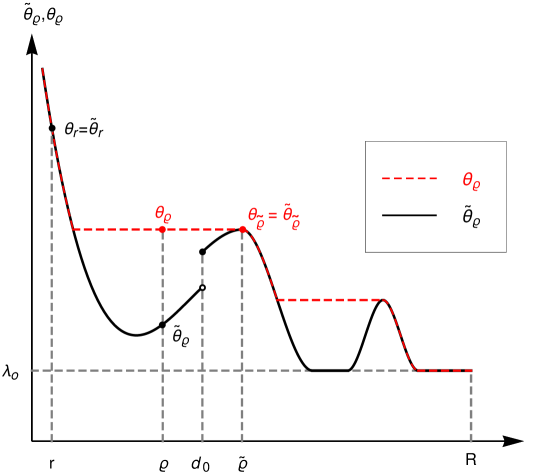
Figure 1. Illustration of the rising sun construction.

Next, we define

(6.10) $$\tilde{\varrho}:=\left\{\begin{array}[]{cl}R&\text{ if }\theta_{\varrho}=\lambda_{o}\vspace{2mm},\\ \min\{s\in[\varrho,R]:\theta_{s}=\tilde{\theta}_{s}\}&\text{ if }\theta_{\varrho}>\lambda_{o},\end{array}\right.$$

i.e. we have $\theta_{r}=\theta_{\tilde{\varrho}}$ for any $r\in[\varrho,\tilde{\varrho}]$.

Lemma 6.2.

• For any $0<\varrho\leq s\leq R$, the constructed cylinders $Q_{s}^{(\theta_{\varrho})}$ are sub-intrinsic in the sense

  $$\left\{\begin{array}[]{ll}\mathchoice{\vbox{\hbox{$\textstyle-\!-$}}\kern-9.58327pt}{\vbox{\hbox{$\scriptstyle-\!-$}}\kern-5.25002pt}{\vbox{\hbox{$\scriptscriptstyle-\!-$}}\kern-3.45834pt}{\vbox{\hbox{$\scriptscriptstyle-\!-$}}\kern-2.70834pt}\!\iint_{Q_{s}^{(\theta_{\varrho})}(z_{o})}\frac{|\hat{u}|^{2m}}{s^{2}}\>\!\mathrm{d}x\>\!\mathrm{d}t\leq\theta_{\varrho}^{2m},&\text{if }s<d_{o},\vspace{2mm}\\ \mathchoice{\vbox{\hbox{$\textstyle-\!-$}}\kern-9.58327pt}{\vbox{\hbox{$\scriptstyle-\!-$}}\kern-5.25002pt}{\vbox{\hbox{$\scriptscriptstyle-\!-$}}\kern-3.45834pt}{\vbox{\hbox{$\scriptscriptstyle-\!-$}}\kern-2.70834pt}\!\iint_{Q_{s}^{(\theta_{\varrho})}(z_{o})}2\frac{|\hat{\bm{u}}^{m}-\hat{\bm{g}}^{m}|^{2}+|\hat{g}|^{2m}}{s^{2}}\>\!\mathrm{d}x\>\!\mathrm{d}t\leq\theta_{\varrho}^{2m},&\text{if }s\geq d_{o}.\end{array}\right.$$

• For any $s\in(\varrho,R]$ we have

  $$\theta_{\varrho}\leq\left(\frac{s}{\varrho}\right)^{\frac{d+2}{m+1}}\theta_{s}.$$

• For any $0<\varrho\leq R$ there holds

  $$\theta_{\varrho}\leq\left(\frac{R}{\varrho}\right)^{\frac{d+2}{m+1}}\theta_{R}\leq\left(\frac{4R}{\varrho}\right)^{\frac{d+2}{m+1}}\lambda_{o}.$$

Proof..

(i) By definition we have $\tilde{\theta}_{s}\leq\theta_{\varrho}$ so that $Q_{s}^{(\theta_{\varrho})}(z_{o})\subset Q_{s}^{(\tilde{\theta}_{s})}(z_{o})$ and therefore if $s<d_{o}$

$$\mathchoice{\vbox{\hbox{$\textstyle-\!-$}}\kern-9.58327pt}{\vbox{\hbox{$\scriptstyle-\!-$}}\kern-5.25002pt}{\vbox{\hbox{$\scriptscriptstyle-\!-$}}\kern-3.45834pt}{\vbox{\hbox{$\scriptscriptstyle-\!-$}}\kern-2.70834pt}\!\iint_{Q_{s}^{(\theta_{\varrho})}(z_{o})}\frac{|\hat{u}|^{2m}}{s^{2}}\>\!\mathrm{d}x\>\!\mathrm{d}t \leq\left(\frac{\theta_{\varrho}}{\tilde{\theta}_{s}}\right)^{m-1}\mathchoice{\vbox{\hbox{$\textstyle-\!-$}}\kern-9.58327pt}{\vbox{\hbox{$\scriptstyle-\!-$}}\kern-5.25002pt}{\vbox{\hbox{$\scriptscriptstyle-\!-$}}\kern-3.45834pt}{\vbox{\hbox{$\scriptscriptstyle-\!-$}}\kern-2.70834pt}\!\iint_{Q_{s}^{(\tilde{\theta}_{s})}(z_{o})}\frac{|\hat{u}|^{2m}}{s^{2}}\>\!\mathrm{d}x\>\!\mathrm{d}t$$

$$\leq\left(\frac{\theta_{\varrho}}{\tilde{\theta}_{s}}\right)^{m-1}\tilde{\theta}_{s}^{2m}=\theta_{\varrho}^{m-1}\tilde{\theta}_{s}^{m+1}\leq\theta_{\varrho}^{2m}.$$

If $s\geq d_{o}$ we obtain

$$\mathchoice{\vbox{\hbox{$\textstyle-\!-$}}\kern-9.58327pt}{\vbox{\hbox{$\scriptstyle-\!-$}}\kern-5.25002pt}{\vbox{\hbox{$\scriptscriptstyle-\!-$}}\kern-3.45834pt}{\vbox{\hbox{$\scriptscriptstyle-\!-$}}\kern-2.70834pt}\!\iint_{Q_{s}^{(\theta_{\varrho})}(z_{o})}2\frac{|\hat{\bm{u}}^{m}-\hat{\bm{g}}^{m}|+|\hat{g}|^{2m}}{s^{2}}\>\!\mathrm{d}x\>\!\mathrm{d}t$$

$$\qquad\leq\left(\frac{\theta_{\varrho}}{\tilde{\theta}_{s}}\right)^{m-1}\mathchoice{\vbox{\hbox{$\textstyle-\!-$}}\kern-9.58327pt}{\vbox{\hbox{$\scriptstyle-\!-$}}\kern-5.25002pt}{\vbox{\hbox{$\scriptscriptstyle-\!-$}}\kern-3.45834pt}{\vbox{\hbox{$\scriptscriptstyle-\!-$}}\kern-2.70834pt}\!\iint_{Q_{s}^{(\tilde{\theta}_{s})}(z_{o})}2\frac{|\hat{\bm{u}}^{m}-\hat{\bm{g}}^{m}|+|\hat{g}|^{2m}}{s^{2}}\>\!\mathrm{d}x\>\!\mathrm{d}t$$

$$\qquad\leq\left(\frac{\theta_{\varrho}}{\tilde{\theta}_{s}}\right)^{m-1}\tilde{\theta}_{s}^{2m}=\theta_{\varrho}^{m-1}\tilde{\theta}_{s}^{m+1}\leq\theta_{\varrho}^{2m}.$$

(ii) If $\theta_{\varrho}=\lambda_{o}$ we know that also $\theta_{s}=\lambda_{o}$, so that the claim holds true. In the case $\theta_{\varrho}>\lambda_{o}$ we first consider radii $s$ with $s\in(\varrho,\tilde{\varrho}]$. Then, $\theta_{\varrho}=\theta_{s}$ and there is nothing to prove. In contrary, if $s\in(\tilde{\varrho},R]$ the monotonicity of $\varrho\mapsto\theta_{\varrho}$, (6.6) and the first part of the Lemma imply in the case $\tilde{\varrho}<d_{o}$

$$\theta_{\varrho} =\tilde{\theta}_{\tilde{\varrho}}=\left[\frac{1}{|Q_{\tilde{\varrho}}|}\iint_{Q_{\tilde{\varrho}}^{(\theta_{\tilde{\varrho}})}(z_{o})}\frac{|\hat{u}|^{2m}}{\tilde{\varrho}^{2}}\>\!\mathrm{d}x\>\!\mathrm{d}t\right]^{\frac{1}{m+1}}$$

$$\leq\left(\frac{s}{\tilde{\varrho}}\right)^{\frac{d+2}{m+1}}\left[\frac{1}{|Q_{s}|}\iint_{Q_{s}^{(\theta_{s})}(z_{o})}\frac{|\hat{u}|^{2m}}{s^{2}}\>\!\mathrm{d}x\>\!\mathrm{d}t\right]^{\frac{1}{m+1}}$$

$$\leq\left(\frac{s}{\varrho}\right)^{\frac{d+2}{m+1}}\theta_{s}.$$

On the other hand, if $\tilde{\varrho}\geq d_{o}$

$$\theta_{\varrho} =\tilde{\theta}_{\tilde{\varrho}}=\left[\frac{1}{|Q_{\tilde{\varrho}}|}\iint_{Q_{\tilde{\varrho}}^{(\theta_{\tilde{\varrho}})}(z_{o})}2\frac{|\hat{\bm{u}}^{m}-\hat{\bm{g}}^{m}|^{2}+|\hat{g}|^{2m}}{\tilde{\varrho}^{2}}\>\!\mathrm{d}x\>\!\mathrm{d}t\right]^{\frac{1}{m+1}}$$

$$\leq\left(\frac{s}{\tilde{\varrho}}\right)^{\frac{d+2}{m+1}}\left[\frac{1}{|Q_{s}|}\iint_{Q_{s}^{(\theta_{s})}(z_{o})}2\frac{|\hat{\bm{u}}^{m}-\hat{\bm{g}}^{m}|^{2}+|\hat{g}|^{2m}}{s^{2}}\>\!\mathrm{d}x\>\!\mathrm{d}t\right]^{\frac{1}{m+1}}$$

$$\leq\left(\frac{s}{\varrho}\right)^{\frac{d+2}{m+1}}\theta_{s}.$$

(iii) Combining (ii) for $s=R$ with estimate (6.7) yields the claim, since $\theta_{R}=\tilde{\theta}_{R}$. ∎

We note that due to the monotonicity of the map $\varrho\mapsto\theta_{\varrho,z_{o}}$ the above constructed cylinders are nested in the sense that

$$Q_{r}^{(\theta_{z_{o},r})}(z_{o})\subset Q_{s}^{(\theta_{z_{o},s})}(z_{o})\quad\text{ whenever }0<r<s\leq R.$$

However, these cylinders in general only fulfill the sub-intrinsic coupling condition from Lemma 6.2 (i).

6.3. Covering property

Next, we will present a Vitali type covering property for the above constructed cylinders. Using the just established bounds from Lemma 6.2, this result can be established by a slight adaptation of the arguments in [4, Lemma 6.1] which is based on the ideas of [15, Lemma 5.2].

Lemma 6.3.

There exists a constant $\hat{c}=\hat{c}(n,m)\geq 160$ such that the following holds true: Let $\mathcal{F}$ be any collection of cylinders $Q_{32r}^{(\theta_{z,r})}(z)$ where $Q_{r}^{(\theta_{z,r})}(z)$ is a cylinder of the form as constructed in section 6.2 with radius $r\in(0,\frac{R}{\hat{c}})$. Then there exists a countable subfamily $\mathcal{G}$ of disjoint cylinders in $\mathcal{F}$ such that

$$\bigcup_{Q\in\mathcal{F}}Q\subset\bigcup_{Q\in\mathcal{G}}\hat{Q},$$

where $\hat{Q}$ denotes the $\frac{\hat{c}}{32}$-times enlarged cylinder $Q$, i.e. if $Q=Q_{32r}^{(\theta_{r,z})}(z)$, then $\hat{Q}=Q_{\hat{c}r}^{(\theta_{z,r})}(z)$.

Proof..

For $j\in\mathbb{N}$ define a sub-collection of $\mathcal{F}$ as

$$\mathcal{F}_{j}:=\big{\{}Q_{32r}^{(\theta_{z;r})}(z)\in\mathcal{F}:\tfrac{R}{2^{j}\hat{c}}<r\leq\tfrac{R}{2^{j-1}\hat{c}}\big{\}}.$$

Next we construct a countable collection of disjoint cylinders $\mathcal{G}\subset\mathcal{F}$ inductively as follows. Let $\mathcal{G}_{1}$ be a maximal disjoint collection of cylinders in $\mathcal{F}_{1}$. Observe that the measure of every cylinder in $\mathcal{G}_{1}$ is bounded from below by Lemma 6.2 (iii), which implies that $\mathcal{G}_{1}$ is finite. For $k\geq 2$, define $\mathcal{G}_{k}$ to be any maximal sub-collection of

$$\bigg{\{}Q\in\mathcal{F}_{k}:Q\cap Q^{\ast}=\emptyset\mbox{ for any $\displaystyle Q^{\ast}\in\bigcup_{j=1}^{k-1}\mathcal{G}_{j}$}\bigg{\}}.$$

Collection $\mathcal{G}_{k}$ is again finite, and we can define

$$\mathcal{G}:=\bigcup_{j\in\mathbb{N}}\mathcal{G}_{j}.$$

Now $\mathcal{G}$ is a countable disjoint sub-collection of $\mathcal{F}$. To conclude the result we show that for any $Q\in\mathcal{F}$ there exists a cylinder $Q^{*}\in\mathcal{G}$ such that $Q\subset\hat{Q}^{*}$.

Fix $Q=Q_{32r}^{(\theta_{z;r})}(z)\in\mathcal{F}$. Then $Q\in\mathcal{F}_{j}$ for some $j\in\mathbb{N}$. Since $\mathcal{G}_{j}$ is maximal, there exists $Q^{*}=Q_{32r_{*}}^{(\theta_{z_{*};r_{*}})}(z_{*})\in\bigcup_{i=1}^{j}\mathcal{G}_{j}$ satisfying $Q\cap Q^{*}\neq\emptyset$. From the definitions it follows that $r\leq\frac{R}{2^{j-1}\hat{c}}$ and $r_{*}>\frac{R}{2^{j}\hat{c}}$, which implies $r\leq 2r_{*}$. Then clearly $B_{32r}(x)\subset B_{160r_{*}}(x_{*})$. The main objective of the rest of the proof is to deduce the inclusion

(6.11) $$\Lambda_{32r}^{(\theta_{z,r})}(t)\subset\Lambda_{\hat{c}r_{*}}^{(\theta_{z_{*},r_{*}})}(t_{*}).$$

Next we show that

(6.12) $$\theta_{z_{*};r_{*}}\leq(4\mu)^{\frac{d+2}{m+1}}\theta_{z;r},$$

where $\mu=128$. By $\tilde{r}_{*}\in[r_{*},R]$ we denote the radius from (6.10) associated to the cylinder $Q_{r_{*}}^{(\theta_{z_{*};r_{*}})}(z_{*})$. Recall that either $Q_{\tilde{r}_{*}}^{(\theta_{z_{*};r_{*}})}(z_{*})$ is intrinsic or $\tilde{r}_{*}=R$ and $\theta_{z_{*};r_{*}}=\lambda_{o}$. In the latter case we have

$$\theta_{z_{*};r_{*}}=\lambda_{o}\leq\theta_{z;r}.$$

Therefore, we can assume that $Q_{\tilde{r}_{*}}^{(\theta_{z_{*};r_{*}})}(z_{*})$ is intrinsic, which means

(6.15) $$\left\{\begin{array}[]{ll}\frac{1}{|Q_{\tilde{r}_{*}}|}\iint_{Q_{\tilde{r}_{*}}^{(\theta_{z_{*};r_{*}})}(z_{*})}\frac{|\hat{u}|^{2m}}{\tilde{r}_{*}^{2}}\>\!\mathrm{d}y\>\!\mathrm{d}\tau=\theta_{z_{*};r_{*}}^{m+1},&\text{if }\tilde{r}_{*}<\frac{1}{2}\operatorname{dist}(x_{*},\partial\Omega)\vspace{2mm}\\ \frac{1}{|Q_{\tilde{r}_{*}}|}\iint_{Q_{\tilde{r}_{*}}^{(\theta_{z_{*},r_{*}})}(z_{*})}2\frac{|\hat{\bm{u}}^{m}-\hat{\bm{g}}^{m}|^{2}+|\hat{g}|^{2m}}{\tilde{r}_{*}^{2}}\>\!\mathrm{d}y\>\!\mathrm{d}\tau=\theta^{m+1}_{z_{*};r_{*}},&\text{if }\tilde{r}_{*}\geq\frac{1}{2}\operatorname{dist}(x_{*},\partial\Omega)\end{array}\right.$$

We first consider the case where $\tilde{r}_{*}>\frac{R}{\mu}$. Here we obtain by triangle inequality in both of the cases $\tilde{r}_{*}<\frac{1}{2}\operatorname{dist}(x_{*},\partial\Omega)$ and $\tilde{r}_{*}\geq\frac{1}{2}\operatorname{dist}(x_{*},\partial\Omega)$ that

$$\theta^{m+1}_{z_{*};r_{*}} =\frac{1}{|Q_{\tilde{r}_{*}}|}\iint_{Q_{\tilde{r}_{*}}^{(\theta_{z_{*},r_{*}})}(z_{*})}2\frac{|\hat{\bm{u}}^{m}-\hat{\bm{g}}^{m}|^{2}+|\hat{g}|^{2m}}{\tilde{r}_{*}^{2}}\>\!\mathrm{d}y\>\!\mathrm{d}\tau$$

$$\leq\left(\frac{4R}{\tilde{r}_{*}}\right)^{2}\frac{1}{|Q_{\tilde{r}_{*}}|}\iint_{Q_{4R}}2\frac{|\hat{\bm{u}}^{m}-\hat{\bm{g}}^{m}|^{2}+|\hat{g}|^{2m}}{(4R)^{2}}\>\!\mathrm{d}y\>\!\mathrm{d}\tau$$

$$\leq\left(\frac{4R}{\tilde{r}_{*}}\right)^{d+2}\lambda_{o}^{m+1}\leq(4\mu)^{d+2}\theta^{m+1}_{z;r}.$$

This shows (6.12) if $\tilde{r}_{*}>\frac{R}{\mu}$. Next, we assume that $\tilde{r}_{*}\leq\frac{R}{\mu}$. We can assume that $\theta_{z;r}\leq\theta_{z_{*};r_{*}}$ since otherwise (6.12) follows directly. Since the cylinders $Q$ and $Q^{*}$ intersect, we have

(6.16) $$|t-t_{*}|\leq\theta_{z;r}^{1-m}(32r)^{\frac{m+1}{m}}+\theta_{z_{*};r_{*}}^{1-m}(32r_{*})^{\frac{m+1}{m}}.$$

Because $\varrho\mapsto\theta_{z;\varrho}$ is decreasing and $r\leq 2r_{*}\leq 2\tilde{r}_{*}\leq\mu\tilde{r}_{*}$, we have that

$$\theta_{z_{*};r_{*}}\geq\theta_{z;r}\geq\theta_{z;\mu\widetilde{r}_{*}}.$$

This implies that

$$\theta_{z_{\ast};r_{*}}^{1-m}(32\widetilde{r}_{*})^{\frac{m+1}{m}}+|t-t_{*}| \leq 2\theta_{z_{*};r_{*}}^{1-m}(32\widetilde{r}_{*})^{\frac{m+1}{m}}+\theta_{z;r}^{1-m}(32r)^{\frac{m+1}{m}}$$

$$\leq 2\cdot 64^{\frac{m+1}{m}}\theta_{z;\mu\widetilde{r}_{*}}^{1-m}\widetilde{r}_{*}^{\frac{m+1}{m}}\leq\theta_{z;\mu\widetilde{r}_{\ast}}^{1-m}(\mu\widetilde{r}_{\ast})^{\frac{m+1}{m}},$$

which shows that

$$\Lambda_{32\tilde{r}_{*}}^{(\theta_{z_{*};r_{*}})}(t_{*})\subset\Lambda_{\mu\tilde{r}_{*}}^{(\theta_{z;\mu\tilde{r}_{*}})}(t)$$

holds true. Since $|x-x_{*}|\leq 96\tilde{r}_{*}$, we also have that $B_{32\tilde{r}_{*}}(x_{*})\subset B_{\mu\tilde{r}_{*}}(x)$. Thus we have the inclusion

(6.17) $$Q_{32\tilde{r}_{*}}^{(\theta_{z_{*};r_{*}})}(z_{*})\subset Q_{\mu\tilde{r}_{*}}^{(\theta_{z;\mu\tilde{r}_{*}})}(z).$$

If $\tilde{r}_{*}\geq\frac{1}{2}\operatorname{dist}(x_{*},\partial\Omega)$, then we also get

$$\frac{1}{2}\operatorname{dist}(x,\partial\Omega) \leq\frac{1}{2}\operatorname{dist}(x_{*},\partial\Omega)+\frac{1}{2}|x-x_{*}|\leq\tilde{r}_{*}+\frac{1}{2}(32r+32r_{*})\leq 49\tilde{r}_{*}\leq\mu\tilde{r}_{*}.$$

Therefore, using the intrinsic scaling and Lemma 6.2 (i) leads to

$$\theta^{m+1}_{z_{*},r_{*}} =\frac{1}{|Q_{\tilde{r}_{*}}|}\iint_{Q_{\tilde{r}_{*}}^{(\theta_{z_{*},r_{*}})}(z_{*})}2\frac{|\hat{\bm{u}}^{m}-\hat{\bm{g}}^{m}|^{2}+|\hat{g}|^{2m}}{\tilde{r}_{*}^{2}}\>\!\mathrm{d}y\>\!\mathrm{d}\tau$$

$$\leq\frac{\mu^{d+2}}{|Q_{\mu\tilde{r}_{*}}|}\iint_{Q_{\mu\tilde{r}_{*}}^{(\theta_{z,\mu\tilde{r}_{*}})}(z)}2\frac{|\hat{\bm{u}}^{m}-\hat{\bm{g}}^{m}|^{2}+|\hat{g}|^{2m}}{(\mu\tilde{r}_{*})^{2}}\>\!\mathrm{d}y\>\!\mathrm{d}\tau$$

$$\leq\mu^{d+2}\theta^{m+1}_{z;\mu\tilde{r}_{*}}\leq\mu^{d+2}\theta^{m+1}_{z;r}.$$

On the other hand if $\tilde{r}_{*}<\frac{1}{2}\operatorname{dist}(x_{*},\partial\Omega)$ we obtain the same estimate. This can be seen as follows: If $\mu\tilde{r}_{*}<\frac{1}{2}\operatorname{dist}(x,\partial\Omega)$ we have

$$\theta^{m+1}_{z_{*},r_{*}} =\frac{1}{|Q_{\tilde{r}_{*}}|}\iint_{Q_{\tilde{r}_{*}}^{(\theta_{z_{*},r_{*}})}(z_{*})}\frac{|\hat{u}|^{2m}}{\tilde{r}_{*}^{2}}\>\!\mathrm{d}y\>\!\mathrm{d}\tau$$

$$\leq\frac{\mu^{d+2}}{|Q_{\mu\tilde{r}_{*}}|}\iint_{Q_{\mu\tilde{r}_{*}}^{(\theta_{z,\mu\tilde{r}_{*}})}(z)}\frac{|\hat{u}|^{2m}}{(\mu\tilde{r}_{*})^{2}}\>\!\mathrm{d}y\>\!\mathrm{d}\tau$$

$$\leq\mu^{d+2}\theta^{m+1}_{z;\mu\tilde{r}_{*}}\leq\mu^{d+2}\theta^{m+1}_{z;r},$$

and for $\mu\tilde{r}_{*}\geq\frac{1}{2}\operatorname{dist}(x,\partial\Omega)$ we can use the triangle inequality to obtain

$$\theta^{m+1}_{z_{*},r_{*}} =\frac{1}{|Q_{\tilde{r}_{*}}|}\iint_{Q_{\tilde{r}_{*}}^{(\theta_{z_{*},r_{*}})}(z_{*})}\frac{|\hat{u}|^{2m}}{\tilde{r}_{*}^{2}}\>\!\mathrm{d}y\>\!\mathrm{d}\tau$$

$$\leq\frac{\mu^{d+2}}{|Q_{\mu\tilde{r}_{*}}|}\iint_{Q_{\mu\tilde{r}_{*}}^{(\theta_{z,\mu\tilde{r}_{*}})}(z)}2\frac{|\hat{\bm{u}}^{m}-\hat{\bm{g}}^{m}|^{2}+|\hat{g}|^{2m}}{(\mu\tilde{r}_{*})^{2}}\>\!\mathrm{d}y\>\!\mathrm{d}\tau$$

$$\leq\mu^{d+2}\theta^{m+1}_{z;\mu\tilde{r}_{*}}\leq\mu^{d+2}\theta^{m+1}_{z;r}.$$

This finally shows (6.12). Now by using (6.16), $r\leq 2r_{*}$ and (6.12) we can estimate

$$\theta_{z;r}^{1-m}(32r)^{\frac{m+1}{m}}+|t-t_{*}| \leq 2\theta_{z;r}^{1-m}(32r)^{\frac{m+1}{m}}+\theta_{z_{*};r_{*}}^{1-m}(32r_{*})^{\frac{m+1}{m}}$$

$$\leq 32^{\frac{m+1}{m}}\Big{[}1+2\cdot 2^{\frac{m+1}{m}}\cdot 512^{\frac{(m-1)(d+2)}{m+1}}\Big{]}\theta_{z_{\ast};r_{\ast}}^{1-m}r_{\ast}^{\frac{m+1}{m}}$$

$$\leq\theta_{z_{\ast};r_{\ast}}^{1-m}(\hat{c}r_{\ast})^{\frac{m+1}{m}},$$

for a constant $\hat{c}=\hat{c}(n,m)>32$, which shows the inclusion (6.11). After possibly enlarging $\hat{c}$ such that $\hat{c}\geq 160$ is satisfied, we have $Q\subset\hat{Q}^{*}$ which completes the proof. ∎

6.4. Stopping time argument

For $\lambda>\lambda_{o}$ and $r\in(0,2R]$ we define the super-level set

$$\mathbf{E}(r,\lambda):=\left\{z\in Q_{r}\cap\Omega_{T}:z\text{ is a Lebesgue point of }|D\bm{u}^{m}|\text{ and }|D\bm{u}^{m}|(z)>\lambda^{m}\right\},$$

where the notion of Lebesgue point has to be understood with respect to the system of cylinders constructed in Section 6.2. Because of the Vitali type covering property from Lemma 6.3, almost every point is a Lebesgue point also in this sense, see [13, 2.9.1]. For fixed $0<R\leq R_{1}<R_{2}\leq 2R$ we consider the cylinders

$$Q_{R}\subseteq Q_{R_{1}}\subset Q_{R_{2}}\subseteq Q_{2R}.$$

Let $z_{o}\in\mathbf{E}(R_{1},\lambda)$. By definition of this set, we have

$$\liminf_{s\downarrow 0}\mathchoice{\vbox{\hbox{$\textstyle-\!-$}}\kern-9.58327pt}{\vbox{\hbox{$\scriptstyle-\!-$}}\kern-5.25002pt}{\vbox{\hbox{$\scriptscriptstyle-\!-$}}\kern-3.45834pt}{\vbox{\hbox{$\scriptscriptstyle-\!-$}}\kern-2.70834pt}\!\iint_{Q_{s}^{(\theta_{s})}(z_{o})}\Big{[}|D\bm{u}^{m}|^{2}\chi_{\Omega_{T}}+G^{2}\Big{]}\>\!\mathrm{d}x\>\!\mathrm{d}t\geq|D\bm{u}^{m}|^{2}(z_{o})>\lambda^{2m}.$$

In the following, we consider values of $\lambda$ satisfying

$$\lambda>B\lambda_{o}\quad\text{ where }\quad B:=\left(\frac{4\hat{c}R}{R_{2}-R_{1}}\right)^{\frac{n+2}{m+1}}>1,$$

in which $\hat{c}$ is the constant from the Vitali covering lemma 6.3. For radii $s$ with

$$\frac{R_{2}-R_{1}}{\hat{c}}\leq s\leq R$$

we obtain by using Lemma 6.2 (iii)

$$\mathchoice{\vbox{\hbox{$\textstyle-\!-$}}\kern-9.58327pt}{\vbox{\hbox{$\scriptstyle-\!-$}}\kern-5.25002pt}{\vbox{\hbox{$\scriptscriptstyle-\!-$}}\kern-3.45834pt}{\vbox{\hbox{$\scriptscriptstyle-\!-$}}\kern-2.70834pt}\!\iint_{Q_{s}^{(\theta_{s})}(z_{o})}\Big{[}|D\bm{u}^{m}|^{2}\chi_{\Omega_{T}}+G^{2}\Big{]}\>\!\mathrm{d}x\>\!\mathrm{d}t \leq\frac{|Q_{4R}|}{|Q_{s}^{(\theta_{s})}|}\mathchoice{\vbox{\hbox{$\textstyle-\!-$}}\kern-9.58327pt}{\vbox{\hbox{$\scriptstyle-\!-$}}\kern-5.25002pt}{\vbox{\hbox{$\scriptscriptstyle-\!-$}}\kern-3.45834pt}{\vbox{\hbox{$\scriptscriptstyle-\!-$}}\kern-2.70834pt}\!\iint_{Q_{4R}}\Big{[}|D\bm{u}^{m}|^{2}\chi_{\Omega_{T}}+G^{2}\Big{]}\>\!\mathrm{d}x\>\!\mathrm{d}t$$

$$\leq\frac{|Q_{4R}|}{|Q_{s}|}\theta_{s}^{m-1}\lambda_{o}^{m+1}$$

$$\leq\left(\frac{4R}{s}\right)^{d+\frac{(d+2)(m-1)}{m+1}}\lambda_{o}^{2m}$$

$$\leq\left(\frac{4\hat{c}R}{R_{2}-R_{1}}\right)^{d+\frac{(d+2)(m-1)}{m+1}}\lambda_{o}^{2m}$$

$$=B^{2m}\lambda_{o}^{2m}<\lambda^{2m}.$$

By absolute continuity of the integral and the continuity of $s\mapsto\theta_{s}$, there exists a maximal radius $\varrho_{z_{o}}\in(0,\frac{R_{2}-R_{1}}{\hat{c}})$ such that

(6.18) $$\mathchoice{\vbox{\hbox{$\textstyle-\!-$}}\kern-9.58327pt}{\vbox{\hbox{$\scriptstyle-\!-$}}\kern-5.25002pt}{\vbox{\hbox{$\scriptscriptstyle-\!-$}}\kern-3.45834pt}{\vbox{\hbox{$\scriptscriptstyle-\!-$}}\kern-2.70834pt}\!\iint_{Q_{\varrho_{z_{o}}}^{(\theta_{\varrho_{z_{o}}})}(z_{o})}\Big{[}|D\bm{u}^{m}|^{2}\chi_{\Omega_{T}}+G^{2}\Big{]}\>\!\mathrm{d}x\>\!\mathrm{d}t=\lambda^{2m}.$$

The maximality of $\varrho_{z_{o}}$ implies

(6.19) $$\mathchoice{\vbox{\hbox{$\textstyle-\!-$}}\kern-9.58327pt}{\vbox{\hbox{$\scriptstyle-\!-$}}\kern-5.25002pt}{\vbox{\hbox{$\scriptscriptstyle-\!-$}}\kern-3.45834pt}{\vbox{\hbox{$\scriptscriptstyle-\!-$}}\kern-2.70834pt}\!\iint_{Q_{s}^{(\theta_{s})}(z_{o})}\Big{[}|D\bm{u}^{m}|^{2}\chi_{\Omega_{T}}+G^{2}\Big{]}\>\!\mathrm{d}x\>\!\mathrm{d}t<\lambda^{2m}$$

for any $s\in(\varrho_{z_{o}},R]$.

6.5. Reverse Hölder inequalities

As before we consider $z_{o}\in\mathbf{E}(R_{1},\lambda)$ and abbreviate $\theta_{\varrho_{z_{o}}}\equiv\theta_{z_{o},\varrho_{z_{o}}}$. From now on we denote the exponent $q<2$ as the maximum of the Sobolev exponents $q$ in Lemma 4.2 and $\frac{2n}{d}$ in Lemma 4.5. We distinguish between the non-degenerate and the degenerate case, which correspond to the cases $\tilde{\varrho}_{z_{o}}\leq 2\varrho_{z_{o}}$ and $\tilde{\varrho}_{z_{o}}>2\varrho_{z_{o}}$.

6.5.1. The non-degenerate case $\tilde{\varrho}_{z_{o}}\leq 2\varrho_{z_{o}}$.

In this case, we note that the cylinder $Q_{\tilde{\varrho}_{z_{o}}}^{(\theta_{\varrho_{z_{o}}})}(z_{o})$ is intrinsic since $\tilde{\varrho}_{z_{o}}<R$. We first consider the boundary case $\tilde{\varrho}_{z_{o}}\geq d_{o}$. Lemma 6.2 (i) and the fact that $Q_{\tilde{\varrho}_{z_{o}}}^{(\theta_{\varrho_{z_{o}}})}(z_{o})$ is intrinsic imply

$$\mathchoice{\vbox{\hbox{$\textstyle-\!-$}}\kern-9.58327pt}{\vbox{\hbox{$\scriptstyle-\!-$}}\kern-5.25002pt}{\vbox{\hbox{$\scriptscriptstyle-\!-$}}\kern-3.45834pt}{\vbox{\hbox{$\scriptscriptstyle-\!-$}}\kern-2.70834pt}\!\iint_{Q_{4\tilde{\varrho}_{z_{o}}}^{(\theta_{\varrho_{z_{o}})}}(z_{o})} 2\frac{|\hat{\bm{u}}^{m}-\hat{\bm{g}}^{m}|^{2}+|\hat{g}|^{2m}}{(4\tilde{\varrho}_{z_{o}})^{2}}\>\!\mathrm{d}x\>\!\mathrm{d}t\leq\theta_{\varrho_{z_{o}}}^{2m}$$

$$\leq 2^{d+2}\mathchoice{\vbox{\hbox{$\textstyle-\!-$}}\kern-9.58327pt}{\vbox{\hbox{$\scriptstyle-\!-$}}\kern-5.25002pt}{\vbox{\hbox{$\scriptscriptstyle-\!-$}}\kern-3.45834pt}{\vbox{\hbox{$\scriptscriptstyle-\!-$}}\kern-2.70834pt}\!\iint_{Q_{2\tilde{\varrho}_{z_{o}}}^{(\theta_{\varrho_{z_{o}})}}(z_{o})}2\frac{|\hat{\bm{u}}^{m}-\hat{\bm{g}}^{m}|^{2}+|\hat{g}|^{2m}}{(2\tilde{\varrho}_{z_{o}})^{2}}\>\!\mathrm{d}x\>\!\mathrm{d}t.$$

Since $\tilde{\varrho}_{z_{o}}\geq d_{o}$, the cylinder $Q_{2\tilde{\varrho}_{z_{o}}}^{(\theta_{\varrho_{z_{o}}})}(z_{o})$ intersects or touches the lateral boundary. Hence, we are in position to use Lemma 5.1 on this cylinder to obtain

$$\frac{1}{|Q_{\varrho_{z_{o}}}^{(\theta_{\varrho_{z_{o}}})}|} \iint_{Q_{\varrho_{z_{o}}}^{(\theta_{\varrho_{z_{o}}})}(z_{o})\cap\Omega_{T}}|D\bm{u}^{m}|^{2}\>\!\mathrm{d}x\>\!\mathrm{d}t$$

$$\leq\frac{c}{|Q_{2\tilde{\varrho}_{z_{o}}}^{(\theta_{\varrho_{z_{o}}})}|}\iint_{Q_{2\tilde{\varrho}_{z_{o}}}^{(\theta_{\varrho_{z_{o}}})}(z_{o})\cap\Omega_{T}}|D\bm{u}^{m}|^{2}\>\!\mathrm{d}x\>\!\mathrm{d}t$$

$$\leq\left(\frac{c}{|Q_{16\tilde{\varrho}_{z_{o}}}^{(\theta_{\varrho_{z_{o}}})}|}\iint_{Q_{16\tilde{\varrho}_{z_{o}}}^{(\theta_{\varrho_{z_{o}}})}(z_{o})\cap\Omega_{T}}|D\bm{u}^{m}|^{q}\>\!\mathrm{d}x\>\!\mathrm{d}t\right)^{\frac{2}{q}}+c\mathchoice{\vbox{\hbox{$\textstyle-\!-$}}\kern-9.58327pt}{\vbox{\hbox{$\scriptstyle-\!-$}}\kern-5.25002pt}{\vbox{\hbox{$\scriptscriptstyle-\!-$}}\kern-3.45834pt}{\vbox{\hbox{$\scriptscriptstyle-\!-$}}\kern-2.70834pt}\!\iint_{Q_{16\tilde{\varrho}_{z_{o}},+}^{(\theta_{\varrho_{z_{o}}})}}G^{2}\>\!\mathrm{d}x\>\!\mathrm{d}t$$

$$\leq\left(\frac{c}{|Q_{32\varrho_{z_{o}}}^{(\theta_{\varrho_{z_{o}}})}|}\iint_{Q_{32\varrho_{z_{o}}}^{(\theta_{\varrho_{z_{o}}})}(z_{o})\cap\Omega_{T}}|D\bm{u}^{m}|^{q}\>\!\mathrm{d}x\>\!\mathrm{d}t\right)^{\frac{2}{q}}+c\mathchoice{\vbox{\hbox{$\textstyle-\!-$}}\kern-9.58327pt}{\vbox{\hbox{$\scriptstyle-\!-$}}\kern-5.25002pt}{\vbox{\hbox{$\scriptscriptstyle-\!-$}}\kern-3.45834pt}{\vbox{\hbox{$\scriptscriptstyle-\!-$}}\kern-2.70834pt}\!\iint_{Q_{32\varrho_{z_{o}},+}^{(\theta_{\varrho_{z_{o}}})}}G^{2}\>\!\mathrm{d}x\>\!\mathrm{d}t,$$

which is the desired reverse Hölder inequality. In the remaining case $\tilde{\varrho}_{z_{o}}<d_{o}$, we are either in the interior case (if $Q_{2\tilde{\varrho}_{z_{o}}}^{(\theta_{\varrho_{z_{o}}})}\Subset\Omega_{T}$) or we might intersect with the initial boundary. Therefore, Lemma 6.2 (i) and the fact that $Q_{\tilde{\varrho}_{z_{o}}}^{(\theta_{\varrho_{z_{o}}})}(z_{o})$ is intrinsic imply

$$\mathchoice{\vbox{\hbox{$\textstyle-\!-$}}\kern-9.58327pt}{\vbox{\hbox{$\scriptstyle-\!-$}}\kern-5.25002pt}{\vbox{\hbox{$\scriptscriptstyle-\!-$}}\kern-3.45834pt}{\vbox{\hbox{$\scriptscriptstyle-\!-$}}\kern-2.70834pt}\!\iint_{Q_{2\tilde{\varrho}_{z_{o}}}^{(\theta_{\varrho_{z_{o}}})}(z_{o})}\frac{|\hat{u}|^{2m}}{(2\tilde{\varrho}_{z_{o}})^{2}}\>\!\mathrm{d}x\>\!\mathrm{d}t\leq\theta_{\varrho_{z_{o}}}^{2m}=\mathchoice{\vbox{\hbox{$\textstyle-\!-$}}\kern-9.58327pt}{\vbox{\hbox{$\scriptstyle-\!-$}}\kern-5.25002pt}{\vbox{\hbox{$\scriptscriptstyle-\!-$}}\kern-3.45834pt}{\vbox{\hbox{$\scriptscriptstyle-\!-$}}\kern-2.70834pt}\!\iint_{Q_{\tilde{\varrho}_{z_{o}}}^{(\theta_{\varrho_{z_{o}}})}(z_{o})}\frac{|\hat{u}|^{2m}}{\tilde{\varrho}_{z_{o}}^{2}}\>\!\mathrm{d}x\>\!\mathrm{d}t,$$

so that the conditions in Lemma 5.3 are satisfied for the cylinder $Q_{\tilde{\varrho}_{z_{o}}}^{(\theta_{\varrho_{z_{o}}})}(z_{o})$. Hence, we obtain

$$\frac{1}{|Q_{\varrho_{z_{o}}}^{(\theta_{\varrho_{z_{o}}})}|} \iint_{Q_{\varrho_{z_{o}},+}^{(\theta_{\varrho_{z_{o}}})}(z_{o})}|D\bm{u}^{m}|^{2}\>\!\mathrm{d}x\>\!\mathrm{d}t$$

$$\leq\frac{c}{|Q_{\tilde{\varrho}_{z_{o}}}^{(\theta_{\varrho_{z_{o}}})}|}\iint_{Q_{\tilde{\varrho}_{z_{o}}}^{(\theta_{\varrho_{z_{o}}})}(z_{o})}|D\hat{\bm{u}}^{m}|^{2}\>\!\mathrm{d}x\>\!\mathrm{d}t$$

$$\leq\left(\frac{c}{|Q_{2\tilde{\varrho}_{z_{o}}}^{(\theta_{\varrho_{z_{o}}})}|}\iint_{Q_{2\tilde{\varrho}_{z_{o}}}^{(\theta_{\varrho_{z_{o}}})}(z_{o})}|D\hat{\bm{u}}^{m}|^{q}\>\!\mathrm{d}x\>\!\mathrm{d}t\right)^{\frac{2}{q}}+c\mathchoice{\vbox{\hbox{$\textstyle-\!-$}}\kern-9.58327pt}{\vbox{\hbox{$\scriptstyle-\!-$}}\kern-5.25002pt}{\vbox{\hbox{$\scriptscriptstyle-\!-$}}\kern-3.45834pt}{\vbox{\hbox{$\scriptscriptstyle-\!-$}}\kern-2.70834pt}\!\iint_{Q_{2\tilde{\varrho}_{z_{o}},+}^{(\theta_{\varrho_{z_{o}}})}}G^{2}\>\!\mathrm{d}x\>\!\mathrm{d}t$$

$$\leq\left(\frac{c}{|Q_{4\varrho_{z_{o}}}^{(\theta_{\varrho_{z_{o}}})}|}\iint_{Q_{4\varrho_{z_{o}}}^{(\theta_{\varrho_{z_{o}}})}(z_{o})}|D\hat{\bm{u}}^{m}|^{q}\>\!\mathrm{d}x\>\!\mathrm{d}t\right)^{\frac{2}{q}}+c\mathchoice{\vbox{\hbox{$\textstyle-\!-$}}\kern-9.58327pt}{\vbox{\hbox{$\scriptstyle-\!-$}}\kern-5.25002pt}{\vbox{\hbox{$\scriptscriptstyle-\!-$}}\kern-3.45834pt}{\vbox{\hbox{$\scriptscriptstyle-\!-$}}\kern-2.70834pt}\!\iint_{Q_{4\varrho_{z_{o}},+}^{(\theta_{\varrho_{z_{o}}})}}G^{2}\>\!\mathrm{d}x\>\!\mathrm{d}t.$$

This completes the treatment of the case $\tilde{\varrho}_{z_{o}}\leq 2\varrho_{z_{o}}$.

6.5.2. The degenerate case $\tilde{\varrho}_{z_{o}}>2\varrho_{z_{o}}$

The main objective in this case is the proof of the claim

(6.20) $$\theta_{\varrho_{z_{o}}}^{2m}\leq c\,\mathchoice{\vbox{\hbox{$\textstyle-\!-$}}\kern-9.58327pt}{\vbox{\hbox{$\scriptstyle-\!-$}}\kern-5.25002pt}{\vbox{\hbox{$\scriptscriptstyle-\!-$}}\kern-3.45834pt}{\vbox{\hbox{$\scriptscriptstyle-\!-$}}\kern-2.70834pt}\!\iint_{Q_{\varrho_{z_{o}}}^{(\theta_{\varrho_{z_{o}}})}(z_{o})}\Big{[}|D\bm{u}^{m}|^{2}\chi_{\Omega_{T}}+G^{2}\Big{]}\>\!\mathrm{d}x\>\!\mathrm{d}t$$

for a universal constant $c$. For the derivation of this property, we distinguish between various cases. First, we observe that in the case $\theta_{\varrho_{z_{o}}}=\lambda_{o}$, the claim is immediate because

$$\theta_{\varrho_{z_{o}}}^{2m}=\lambda_{o}^{2m}<\lambda^{2m}=\mathchoice{\vbox{\hbox{$\textstyle-\!-$}}\kern-9.58327pt}{\vbox{\hbox{$\scriptstyle-\!-$}}\kern-5.25002pt}{\vbox{\hbox{$\scriptscriptstyle-\!-$}}\kern-3.45834pt}{\vbox{\hbox{$\scriptscriptstyle-\!-$}}\kern-2.70834pt}\!\iint_{Q_{\varrho_{z_{o}}}^{(\theta_{\varrho_{z_{o}}})}(z_{o})}\Big{[}|D\bm{u}^{m}|^{2}\chi_{\Omega_{T}}+G^{2}\Big{]}\>\!\mathrm{d}x\>\!\mathrm{d}t$$

by (6.18). Therefore, we may assume that $\theta_{\varrho_{z_{o}}}>\lambda_{o}$, in which case the cylinder $Q_{\tilde{\varrho}_{z_{o}}}^{(\theta_{\varrho_{z_{o}}})}(z_{o})$ is intrinsic. We first consider the case $\tilde{\varrho}_{z_{o}}<d_{o}$. We use the Poincaré inequality from Lemma 4.5, inequality (6.19) and Lemma 6.2 (i) with $s=\frac{1}{2}\tilde{\varrho}_{z_{o}}>\varrho_{z_{o}}$ to obtain

$$\theta_{\varrho_{z_{o}}}^{m} =\left[\mathchoice{\vbox{\hbox{$\textstyle-\!-$}}\kern-9.58327pt}{\vbox{\hbox{$\scriptstyle-\!-$}}\kern-5.25002pt}{\vbox{\hbox{$\scriptscriptstyle-\!-$}}\kern-3.45834pt}{\vbox{\hbox{$\scriptscriptstyle-\!-$}}\kern-2.70834pt}\!\iint_{Q_{\tilde{\varrho}_{z_{o}}}^{(\theta_{\varrho_{z_{o}}})}(z_{o})}\frac{|\hat{u}|^{2m}}{\tilde{\varrho}_{z_{o}}^{2}}\>\!\mathrm{d}x\>\!\mathrm{d}t\right]^{\frac{1}{2}}$$

$$\leq\left[\mathchoice{\vbox{\hbox{$\textstyle-\!-$}}\kern-9.58327pt}{\vbox{\hbox{$\scriptstyle-\!-$}}\kern-5.25002pt}{\vbox{\hbox{$\scriptscriptstyle-\!-$}}\kern-3.45834pt}{\vbox{\hbox{$\scriptscriptstyle-\!-$}}\kern-2.70834pt}\!\iint_{Q_{\tilde{\varrho}_{z_{o}}}^{(\theta_{\varrho_{z_{o}}})}(z_{o})}\frac{\big{|}\hat{\bm{u}}^{m}-(\hat{\bm{u}}^{m})_{z_{o};\frac{1}{2}\tilde{\varrho}_{z_{o}}}^{(\theta_{\varrho_{z_{o}}})}\big{|}^{2}}{\tilde{\varrho}_{z_{o}}^{2}}\>\!\mathrm{d}x\>\!\mathrm{d}t\right]^{\frac{1}{2}}+\frac{\big{|}(\hat{\bm{u}}^{m})_{z_{o};\frac{1}{2}\tilde{\varrho}_{z_{o}}}^{(\theta_{\varrho_{z_{o}}})}\big{|}}{\tilde{\varrho}_{z_{o}}}$$

$$\leq c\left[\mathchoice{\vbox{\hbox{$\textstyle-\!-$}}\kern-9.58327pt}{\vbox{\hbox{$\scriptstyle-\!-$}}\kern-5.25002pt}{\vbox{\hbox{$\scriptscriptstyle-\!-$}}\kern-3.45834pt}{\vbox{\hbox{$\scriptscriptstyle-\!-$}}\kern-2.70834pt}\!\iint_{Q_{\tilde{\varrho}_{z_{o}}}^{(\theta_{\varrho_{z_{o}}})}(z_{o})}\Big{[}|D\bm{u}^{m}|^{2}\chi_{\Omega_{T}}+G^{2}\Big{]}\>\!\mathrm{d}x\>\!\mathrm{d}t\right]^{\frac{1}{2}}+\mathchoice{\vbox{\hbox{$\textstyle-\!-$}}\kern-9.58327pt}{\vbox{\hbox{$\scriptstyle-\!-$}}\kern-5.25002pt}{\vbox{\hbox{$\scriptscriptstyle-\!-$}}\kern-3.45834pt}{\vbox{\hbox{$\scriptscriptstyle-\!-$}}\kern-2.70834pt}\!\iint_{Q_{\frac{1}{2}\tilde{\varrho}_{z_{o}}}^{(\theta_{\varrho_{z_{o}}})}(z_{o})}\frac{|\hat{u}|^{m}}{\tilde{\varrho}_{z_{o}}}\>\!\mathrm{d}x\>\!\mathrm{d}t$$

$$\leq c\lambda^{m}+\tfrac{1}{2}\left[\mathchoice{\vbox{\hbox{$\textstyle-\!-$}}\kern-9.58327pt}{\vbox{\hbox{$\scriptstyle-\!-$}}\kern-5.25002pt}{\vbox{\hbox{$\scriptscriptstyle-\!-$}}\kern-3.45834pt}{\vbox{\hbox{$\scriptscriptstyle-\!-$}}\kern-2.70834pt}\!\iint_{Q_{\frac{1}{2}\tilde{\varrho}_{z_{o}}}^{(\theta_{\varrho_{z_{o}}})}(z_{o})}\frac{|\hat{u}|^{2m}}{(\frac{1}{2}\tilde{\varrho}_{z_{o}})^{2}}\>\!\mathrm{d}x\>\!\mathrm{d}t\right]^{\frac{1}{2}}$$

$$\leq c\lambda^{m}+\tfrac{1}{2}\theta_{\varrho_{z_{o}}}^{m}.$$

This implies $\theta_{\varrho_{z_{o}}}^{2m}\leq c\lambda^{2m}$, which in turn yields claim (6.20) in view of property (6.18). Next, we turn our attention to the case $\tilde{\varrho}_{z_{o}}\geq d_{o}$. Now we use Lemma 4.1 on the cylinder $Q_{8\tilde{\varrho}_{z_{o}}}^{(\theta_{\tilde{\varrho}_{z_{o}}})}(z_{o})$, which is possible since $\tilde{\varrho}_{z_{o}}\geq d_{o}$ implies $B_{8\tilde{\varrho}_{z_{o}}/3}\setminus\Omega\neq\emptyset$. Moreover, we use Lemmas 2.4 and 4.3 and then inequality (6.19). This leads us to the estimate

(6.21) $$\theta_{\varrho_{z_{o}}}^{m} =\left[\mathchoice{\vbox{\hbox{$\textstyle-\!-$}}\kern-9.58327pt}{\vbox{\hbox{$\scriptstyle-\!-$}}\kern-5.25002pt}{\vbox{\hbox{$\scriptscriptstyle-\!-$}}\kern-3.45834pt}{\vbox{\hbox{$\scriptscriptstyle-\!-$}}\kern-2.70834pt}\!\iint_{Q_{\tilde{\varrho}_{z_{o}}}^{(\theta_{\varrho_{z_{o}}})}(z_{o})}2\frac{|\hat{\bm{u}}^{m}-\hat{\bm{g}}^{m}|^{2}+|\hat{g}|^{2m}}{\tilde{\varrho}_{z_{o}}^{2}}\>\!\mathrm{d}x\>\!\mathrm{d}t\right]^{\frac{1}{2}}$$

$$\leq\left[\mathchoice{\vbox{\hbox{$\textstyle-\!-$}}\kern-9.58327pt}{\vbox{\hbox{$\scriptstyle-\!-$}}\kern-5.25002pt}{\vbox{\hbox{$\scriptscriptstyle-\!-$}}\kern-3.45834pt}{\vbox{\hbox{$\scriptscriptstyle-\!-$}}\kern-2.70834pt}\!\iint_{Q_{\tilde{\varrho}_{z_{o}}}^{(\theta_{\varrho_{z_{o}}})}(z_{o})}2\frac{|\hat{\bm{u}}^{m}-\hat{\bm{g}}^{m}|^{2}}{\tilde{\varrho}_{z_{o}}^{2}}\>\!\mathrm{d}x\>\!\mathrm{d}t\right]^{\frac{1}{2}}$$

$$\quad+\left[\mathchoice{\vbox{\hbox{$\textstyle-\!-$}}\kern-9.58327pt}{\vbox{\hbox{$\scriptstyle-\!-$}}\kern-5.25002pt}{\vbox{\hbox{$\scriptscriptstyle-\!-$}}\kern-3.45834pt}{\vbox{\hbox{$\scriptscriptstyle-\!-$}}\kern-2.70834pt}\!\iint_{Q_{\tilde{\varrho}_{z_{o}}}^{(\theta_{\varrho_{z_{o}}})}(z_{o})}2\frac{\big{|}\hat{\bm{g}}^{m}-(\hat{\bm{g}}^{m})_{z_{o};\frac{1}{2}\tilde{\varrho}_{z_{o}}}^{(\theta_{\varrho_{z_{o}}})}\big{|}^{2}}{\tilde{\varrho}_{z_{o}}^{2}}\>\!\mathrm{d}x\>\!\mathrm{d}t\right]^{\frac{1}{2}}+\sqrt{2}\,\frac{\big{|}(\hat{\bm{g}}^{m})_{z_{o};\frac{1}{2}\tilde{\varrho}_{z_{o}}}^{(\theta_{\varrho_{z_{o}}})}\big{|}}{\tilde{\varrho}_{z_{o}}}$$

$$\leq c\left[\mathchoice{\vbox{\hbox{$\textstyle-\!-$}}\kern-9.58327pt}{\vbox{\hbox{$\scriptstyle-\!-$}}\kern-5.25002pt}{\vbox{\hbox{$\scriptscriptstyle-\!-$}}\kern-3.45834pt}{\vbox{\hbox{$\scriptscriptstyle-\!-$}}\kern-2.70834pt}\!\iint_{Q_{8\tilde{\varrho}_{z_{o}}}^{(\theta_{8\tilde{\varrho}_{z_{o}}})}(z_{o})}\Big{[}|D\bm{u}^{m}|^{2}\chi_{\Omega_{T}}+G^{2}\Big{]}\>\!\mathrm{d}x\>\!\mathrm{d}t\right]^{\frac{1}{2}}+\tfrac{1}{2}\left[\mathchoice{\vbox{\hbox{$\textstyle-\!-$}}\kern-9.58327pt}{\vbox{\hbox{$\scriptstyle-\!-$}}\kern-5.25002pt}{\vbox{\hbox{$\scriptscriptstyle-\!-$}}\kern-3.45834pt}{\vbox{\hbox{$\scriptscriptstyle-\!-$}}\kern-2.70834pt}\!\iint_{Q_{\frac{1}{2}\tilde{\varrho}_{z_{o}}}^{(\theta_{\varrho_{z_{o}}})}(z_{o})}2\frac{|\hat{g}|^{2m}}{(\frac{1}{2}\tilde{\varrho}_{z_{o}})^{2}}\>\!\mathrm{d}x\>\!\mathrm{d}t\right]^{\frac{1}{2}}$$

$$\leq c\lambda^{m}+\tfrac{1}{2}\left[\mathchoice{\vbox{\hbox{$\textstyle-\!-$}}\kern-9.58327pt}{\vbox{\hbox{$\scriptstyle-\!-$}}\kern-5.25002pt}{\vbox{\hbox{$\scriptscriptstyle-\!-$}}\kern-3.45834pt}{\vbox{\hbox{$\scriptscriptstyle-\!-$}}\kern-2.70834pt}\!\iint_{Q_{\frac{1}{2}\tilde{\varrho}_{z_{o}}}^{(\theta_{\varrho_{z_{o}}})}(z_{o})}2\frac{|\hat{g}|^{2m}}{(\frac{1}{2}\tilde{\varrho}_{z_{o}})^{2}}\>\!\mathrm{d}x\>\!\mathrm{d}t\right]^{\frac{1}{2}}.$$

For the estimate of the last integral, we distinguish further between the cases $\frac{1}{2}\tilde{\varrho}_{z_{o}}\geq d_{o}$ and $\frac{1}{2}\tilde{\varrho}_{z_{o}}<d_{o}\leq\tilde{\varrho}_{z_{o}}$. In the first case, Lemma 6.2 (i) with $s=\frac{1}{2}\tilde{\varrho}_{z_{o}}\geq\varrho_{z_{o}}$, which satisfies $s\geq d_{o}$, yields

$$\tfrac{1}{2}\left[\mathchoice{\vbox{\hbox{$\textstyle-\!-$}}\kern-9.58327pt}{\vbox{\hbox{$\scriptstyle-\!-$}}\kern-5.25002pt}{\vbox{\hbox{$\scriptscriptstyle-\!-$}}\kern-3.45834pt}{\vbox{\hbox{$\scriptscriptstyle-\!-$}}\kern-2.70834pt}\!\iint_{Q_{\frac{1}{2}\tilde{\varrho}_{z_{o}}}^{(\theta_{\varrho_{z_{o}}})}(z_{o})}2\frac{|\hat{g}|^{2m}}{(\frac{1}{2}\tilde{\varrho}_{z_{o}})^{2}}\>\!\mathrm{d}x\>\!\mathrm{d}t\right]^{\frac{1}{2}}\leq\tfrac{1}{2}\theta_{\varrho_{z_{o}}}^{m}.$$

In the second case $\frac{1}{2}\tilde{\varrho}_{z_{o}}<d_{o}\leq\tilde{\varrho}_{z_{o}}$, we estimate

$$\tfrac{1}{2}\left[\mathchoice{\vbox{\hbox{$\textstyle-\!-$}}\kern-9.58327pt}{\vbox{\hbox{$\scriptstyle-\!-$}}\kern-5.25002pt}{\vbox{\hbox{$\scriptscriptstyle-\!-$}}\kern-3.45834pt}{\vbox{\hbox{$\scriptscriptstyle-\!-$}}\kern-2.70834pt}\!\iint_{Q_{\frac{1}{2}\tilde{\varrho}_{z_{o}}}^{(\theta_{\varrho_{z_{o}}})}(z_{o})}2\frac{|\hat{g}|^{2m}}{(\frac{1}{2}\tilde{\varrho}_{z_{o}})^{2}}\>\!\mathrm{d}x\>\!\mathrm{d}t\right]^{\frac{1}{2}}$$

$$\qquad\leq\tfrac{1}{2}\left[\mathchoice{\vbox{\hbox{$\textstyle-\!-$}}\kern-9.58327pt}{\vbox{\hbox{$\scriptstyle-\!-$}}\kern-5.25002pt}{\vbox{\hbox{$\scriptscriptstyle-\!-$}}\kern-3.45834pt}{\vbox{\hbox{$\scriptscriptstyle-\!-$}}\kern-2.70834pt}\!\iint_{Q_{\frac{1}{2}\tilde{\varrho}_{z_{o}}}^{(\theta_{\varrho_{z_{o}}})}(z_{o})}2\frac{|\hat{\bm{g}}^{m}-\hat{\bm{u}}^{m}|^{2}}{(\frac{1}{2}\tilde{\varrho}_{z_{o}})^{2}}\>\!\mathrm{d}x\>\!\mathrm{d}t\right]^{\frac{1}{2}}+\tfrac{1}{\sqrt{2}}\left[\mathchoice{\vbox{\hbox{$\textstyle-\!-$}}\kern-9.58327pt}{\vbox{\hbox{$\scriptstyle-\!-$}}\kern-5.25002pt}{\vbox{\hbox{$\scriptscriptstyle-\!-$}}\kern-3.45834pt}{\vbox{\hbox{$\scriptscriptstyle-\!-$}}\kern-2.70834pt}\!\iint_{Q_{\frac{1}{2}\tilde{\varrho}_{z_{o}}}^{(\theta_{\varrho_{z_{o}}})}(z_{o})}\frac{|\hat{u}|^{2m}}{(\frac{1}{2}\tilde{\varrho}_{z_{o}})^{2}}\>\!\mathrm{d}x\>\!\mathrm{d}t\right]^{\frac{1}{2}}$$

$$\qquad\leq c\left[\mathchoice{\vbox{\hbox{$\textstyle-\!-$}}\kern-9.58327pt}{\vbox{\hbox{$\scriptstyle-\!-$}}\kern-5.25002pt}{\vbox{\hbox{$\scriptscriptstyle-\!-$}}\kern-3.45834pt}{\vbox{\hbox{$\scriptscriptstyle-\!-$}}\kern-2.70834pt}\!\iint_{Q_{8\tilde{\varrho}_{z_{o}}}^{(\theta_{8\tilde{\varrho}_{z_{o}}})}(z_{o})}\Big{[}|D\bm{u}^{m}|^{2}\chi_{\Omega_{T}}+G^{2}\Big{]}\>\!\mathrm{d}x\>\!\mathrm{d}t\right]^{\frac{1}{2}}+\tfrac{1}{\sqrt{2}}\,\theta_{\varrho_{z_{o}}}^{m}$$

$$\qquad\leq c\lambda^{m}+\tfrac{1}{\sqrt{2}}\,\theta_{\varrho_{z_{o}}}^{m},$$

where we applied Lemma 4.1 on $Q_{8\tilde{\varrho}_{z_{o}}}^{(\theta_{\tilde{\varrho}_{z_{o}}})}(z_{o})$, Lemma 6.2 (i) with $s=\frac{1}{2}\tilde{\varrho}_{z_{o}}<d_{o}$ and (6.19). In view of the last two estimates, we infer from (6.21) that in both cases, we have

$$\theta_{\varrho_{z_{o}}}^{m}\leq c\lambda^{m}+\tfrac{1}{\sqrt{2}}\,\theta_{\varrho_{z_{o}}}^{m}.$$

By absorbing $\tfrac{1}{\sqrt{2}}\,\theta_{\varrho_{z_{o}}}^{m}$ into the left-hand side and recalling (6.18), we obtain the claim (6.20) in the remaining case $\tilde{\varrho}_{z_{o}}\geq d_{o}$. Hence, we have established (6.20) in any case.

Now we are in position to derive the reverse Hölder inequality in the degenerate case. If $\varrho_{z_{o}}<d_{o}$, we observe that Lemma 6.2 (i) implies

$$\mathchoice{\vbox{\hbox{$\textstyle-\!-$}}\kern-9.58327pt}{\vbox{\hbox{$\scriptstyle-\!-$}}\kern-5.25002pt}{\vbox{\hbox{$\scriptscriptstyle-\!-$}}\kern-3.45834pt}{\vbox{\hbox{$\scriptscriptstyle-\!-$}}\kern-2.70834pt}\!\iint_{Q_{2\varrho_{z_{o}}}^{(\theta_{\varrho_{z_{o}}})}}\frac{|\hat{u}|^{2m}}{(2\varrho_{z_{o}})^{2}}\>\!\mathrm{d}x\>\!\mathrm{d}t\leq\theta_{\varrho_{z_{o}}}^{2m}.$$

Combined with (6.20) and the fact $B_{2\varrho_{z_{o}}}(x_{o})\subset\Omega$, this shows that the assumptions of Lemma 5.4 are satisfied, which provides us with the reverse Hölder inequality

$$\frac{1}{|Q_{\varrho_{z_{o}}}^{(\theta_{\varrho_{z_{o}}})}|} \iint_{Q_{\varrho_{z_{o}}}^{(\theta_{\varrho_{z_{o}}})}(z_{o})}|D\hat{\bm{u}}^{m}|^{2}\>\!\mathrm{d}x\>\!\mathrm{d}t$$

$$\leq\left(\frac{c}{|Q_{2\varrho_{z_{o}}}^{(\theta_{\varrho_{z_{o}}})}|}\iint_{Q_{2\varrho_{z_{o}}}^{(\theta_{\varrho_{z_{o}}})}(z_{o})}|D\hat{\bm{u}}^{m}|^{q}\>\!\mathrm{d}x\>\!\mathrm{d}t\right)^{\frac{2}{q}}+c\,\mathchoice{\vbox{\hbox{$\textstyle-\!-$}}\kern-9.58327pt}{\vbox{\hbox{$\scriptstyle-\!-$}}\kern-5.25002pt}{\vbox{\hbox{$\scriptscriptstyle-\!-$}}\kern-3.45834pt}{\vbox{\hbox{$\scriptscriptstyle-\!-$}}\kern-2.70834pt}\!\iint_{Q_{2\varrho_{z_{o}},+}^{(\theta_{\varrho_{z_{o}}})}}G^{2}\>\!\mathrm{d}x\>\!\mathrm{d}t.$$

On the other hand if $\varrho_{z_{o}}\geq d_{o}$, we infer from Lemma 6.2 (i) that

$$\mathchoice{\vbox{\hbox{$\textstyle-\!-$}}\kern-9.58327pt}{\vbox{\hbox{$\scriptstyle-\!-$}}\kern-5.25002pt}{\vbox{\hbox{$\scriptscriptstyle-\!-$}}\kern-3.45834pt}{\vbox{\hbox{$\scriptscriptstyle-\!-$}}\kern-2.70834pt}\!\iint_{Q_{4\varrho_{z_{o}}}^{(\theta_{\varrho_{z_{o}}})}}2\frac{|\hat{\bm{u}}^{m}-\hat{\bm{g}}^{m}|^{2}+|\hat{g}|^{2m}}{(4\varrho_{z_{o}})^{2}}\>\!\mathrm{d}x\>\!\mathrm{d}t\leq\theta_{\varrho_{z_{o}}}^{2m}.$$

Because of (6.20) and $\varrho_{z_{o}}\geq d_{o}$, we can thus apply Lemma 5.2 with $\varrho=2\varrho_{z_{o}}$ and obtain

$$\frac{1}{|Q_{\varrho_{z_{o}}}^{(\theta_{\varrho_{z_{o}}})}|} \iint_{Q_{\varrho_{z_{o}}}^{(\theta_{\varrho_{z_{o}}})}(z_{o})\cap\Omega_{T}}|D\bm{u}^{m}|^{2}\>\!\mathrm{d}x\>\!\mathrm{d}t$$

$$\leq\frac{c}{|Q_{2\varrho_{z_{o}}}^{(\theta_{\varrho_{z_{o}}})}|}\iint_{Q_{2\varrho_{z_{o}}}^{(\theta_{\varrho_{z_{o}}})}(z_{o})\cap\Omega_{T}}|D\bm{u}^{m}|^{2}\>\!\mathrm{d}x\>\!\mathrm{d}t$$

$$\leq\left(\frac{c}{|Q_{16\varrho_{z_{o}}}^{(\theta_{\varrho_{z_{o}}})}|}\iint_{Q_{16\varrho_{z_{o}}}^{(\theta_{\varrho_{z_{o}}})}(z_{o})\cap\Omega_{T}}|D\bm{u}^{m}|^{q}\>\!\mathrm{d}x\>\!\mathrm{d}t\right)^{\frac{2}{q}}+c\,\mathchoice{\vbox{\hbox{$\textstyle-\!-$}}\kern-9.58327pt}{\vbox{\hbox{$\scriptstyle-\!-$}}\kern-5.25002pt}{\vbox{\hbox{$\scriptscriptstyle-\!-$}}\kern-3.45834pt}{\vbox{\hbox{$\scriptscriptstyle-\!-$}}\kern-2.70834pt}\!\iint_{Q_{16\varrho_{z_{o}},+}^{(\theta_{\varrho_{z_{o}}})}}G^{2}\>\!\mathrm{d}x\>\!\mathrm{d}t.$$

This concludes the proof for the degenerate case. In summary, in any case we have established the reverse Hölder inequality

$$\frac{1}{\big{|}Q_{\varrho_{z_{o}}}^{(\theta_{\varrho_{z_{o}}})}\big{|}} \iint_{Q_{\varrho_{z_{o}}}^{(\theta_{\varrho_{z_{o}}})}(z_{o})\cap\Omega_{T}}|D\bm{u}^{m}|^{2}\>\!\mathrm{d}x\>\!\mathrm{d}t$$

(6.22) $$\leq\left(\frac{c}{\big{|}Q_{32\varrho_{z_{o}}}^{(\theta_{\varrho_{z_{o}}})}\big{|}}\iint_{Q_{32\varrho_{z_{o}}}^{(\theta_{\varrho_{z_{o}}})}(z_{o})\cap\Omega_{T}}|D\bm{u}^{m}|^{q}\>\!\mathrm{d}x\>\!\mathrm{d}t\right)^{\frac{2}{q}}+c\mathchoice{\vbox{\hbox{$\textstyle-\!-$}}\kern-9.58327pt}{\vbox{\hbox{$\scriptstyle-\!-$}}\kern-5.25002pt}{\vbox{\hbox{$\scriptscriptstyle-\!-$}}\kern-3.45834pt}{\vbox{\hbox{$\scriptscriptstyle-\!-$}}\kern-2.70834pt}\!\iint_{Q_{32\varrho_{z_{o}},+}^{(\theta_{\varrho_{z_{o}}})}}G^{2}\>\!\mathrm{d}x\>\!\mathrm{d}t.$$

6.6. Estimate on super-level sets

We define the super-level set for function $G$ as

$$\mathbf{G}(r,\lambda):=\left\{z\in Q_{r}:z\text{ is a Lebesgue point of }G\text{ and }|G(z)|>\lambda^{m}\right\}.$$

For $\eta\in(0,1]$ we have

$$\lambda^{2m} =\mathchoice{\vbox{\hbox{$\textstyle-\!-$}}\kern-9.58327pt}{\vbox{\hbox{$\scriptstyle-\!-$}}\kern-5.25002pt}{\vbox{\hbox{$\scriptscriptstyle-\!-$}}\kern-3.45834pt}{\vbox{\hbox{$\scriptscriptstyle-\!-$}}\kern-2.70834pt}\!\iint_{Q_{\varrho_{z_{o}}}^{(\theta_{\varrho_{z_{o}}})}(z_{o})}\Big{[}|D\bm{u}^{m}|^{2}\chi_{\Omega_{T}}+G^{2}\Big{]}\>\!\mathrm{d}x\>\!\mathrm{d}t$$

$$\leq c\left(\mathchoice{\vbox{\hbox{$\textstyle-\!-$}}\kern-9.58327pt}{\vbox{\hbox{$\scriptstyle-\!-$}}\kern-5.25002pt}{\vbox{\hbox{$\scriptscriptstyle-\!-$}}\kern-3.45834pt}{\vbox{\hbox{$\scriptscriptstyle-\!-$}}\kern-2.70834pt}\!\iint_{Q_{32\varrho_{z_{o}}}^{(\theta_{\varrho_{z_{o}}})}(z_{o})}|D\bm{u}^{m}|^{q}\chi_{\Omega_{T}}\>\!\mathrm{d}x\>\!\mathrm{d}t\right)^{\frac{2}{q}}+c\,\mathchoice{\vbox{\hbox{$\textstyle-\!-$}}\kern-9.58327pt}{\vbox{\hbox{$\scriptstyle-\!-$}}\kern-5.25002pt}{\vbox{\hbox{$\scriptscriptstyle-\!-$}}\kern-3.45834pt}{\vbox{\hbox{$\scriptscriptstyle-\!-$}}\kern-2.70834pt}\!\iint_{Q_{32\varrho_{z_{o}},+}^{(\theta_{\varrho_{z_{o}}})}}G^{2}\>\!\mathrm{d}x\>\!\mathrm{d}t$$

$$\leq c\eta^{2m}\lambda^{2m}+\left(\frac{c}{\big{|}Q_{32\varrho_{z_{o}}}^{(\theta_{\varrho_{z_{o}}})}\big{|}}\iint_{Q_{32\varrho_{z_{o}}}^{(\theta_{\varrho_{z_{o}}})}(z_{o})\cap\mathbf{E}(R_{2},\eta\lambda)}|D\bm{u}^{m}|^{q}\>\!\mathrm{d}x\>\!\mathrm{d}t\right)^{\frac{2}{q}}$$

$$\quad+\frac{c}{\big{|}Q_{32\varrho_{z_{o}}}^{(\theta_{\varrho_{z_{o}}})}\big{|}}\iint_{Q_{32\varrho_{z_{o}},+}^{(\theta_{\varrho_{z_{o}}})}\cap\mathbf{G}(R_{2},\eta\lambda)}G^{2}\>\!\mathrm{d}x\>\!\mathrm{d}t,$$

by using (6.18) and (6.5.2). Now by choosing $\eta^{2m}=\frac{1}{2c}$ we can absorb the first term into the left-hand side. In order to treat the second term we estimate

$$\Bigg{(}\frac{c}{\big{|}Q_{32\varrho_{z_{o}}}^{(\theta_{\varrho_{z_{o}}})}\big{|}} \iint_{Q_{32\varrho_{z_{o}}}^{(\theta_{\varrho_{z_{o}}})}(z_{o})\cap\mathbf{E}(R_{2},\eta\lambda)}|D\bm{u}^{m}|^{q}\>\!\mathrm{d}x\>\!\mathrm{d}t\Bigg{)}^{\frac{2}{q}-1}$$

$$\leq\left(\mathchoice{\vbox{\hbox{$\textstyle-\!-$}}\kern-9.58327pt}{\vbox{\hbox{$\scriptstyle-\!-$}}\kern-5.25002pt}{\vbox{\hbox{$\scriptscriptstyle-\!-$}}\kern-3.45834pt}{\vbox{\hbox{$\scriptscriptstyle-\!-$}}\kern-2.70834pt}\!\iint_{Q_{32\varrho_{z_{o}}}^{(\theta_{\varrho_{z_{o}}})}(z_{o})}|D\bm{u}^{m}|^{2}\chi_{\Omega_{T}}\>\!\mathrm{d}x\>\!\mathrm{d}t\right)^{1-\frac{q}{2}}$$

$$\leq c\lambda^{m(2-q)},$$

where we used Hölder’s inequality and inequality (6.19). Collecting the estimates above we have

$$\lambda^{2m}\big{|}Q_{32\varrho_{z_{o}}}^{(\theta_{\varrho_{z_{o}}})}\big{|}\leq c \iint_{Q_{32\varrho_{z_{o}}}^{(\theta_{\varrho_{z_{o}}})}(z_{o})\cap\mathbf{E}(R_{2},\eta\lambda)}\lambda^{m(2-q)}\big{|}D\bm{u}^{m}\big{|}^{2}\>\!\mathrm{d}x\>\!\mathrm{d}t$$

$$+c\iint_{Q_{32\varrho_{z_{o}},+}^{(\theta_{\varrho_{z_{o}}})}\cap\mathbf{G}(R_{2},\eta\lambda)}G^{2}\>\!\mathrm{d}x\>\!\mathrm{d}t.$$

On the other hand, inequality (6.19), the monotonicity of the mapping $\varrho\mapsto\theta_{\varrho}$ and Lemma 6.2 (ii) imply that

$$\lambda^{2m}>\mathchoice{\vbox{\hbox{$\textstyle-\!-$}}\kern-9.58327pt}{\vbox{\hbox{$\scriptstyle-\!-$}}\kern-5.25002pt}{\vbox{\hbox{$\scriptscriptstyle-\!-$}}\kern-3.45834pt}{\vbox{\hbox{$\scriptscriptstyle-\!-$}}\kern-2.70834pt}\!\iint_{Q_{\hat{c}\varrho_{z_{o}}}^{(\theta_{\hat{c}\varrho_{z_{o}}})}(z_{o})}|D\bm{u}^{m}|^{2}\chi_{\Omega_{T}}\,\>\!\mathrm{d}x\>\!\mathrm{d}t\geq\hat{c}^{\frac{(1-m)(d+2)}{m+1}}\mathchoice{\vbox{\hbox{$\textstyle-\!-$}}\kern-9.58327pt}{\vbox{\hbox{$\scriptstyle-\!-$}}\kern-5.25002pt}{\vbox{\hbox{$\scriptscriptstyle-\!-$}}\kern-3.45834pt}{\vbox{\hbox{$\scriptscriptstyle-\!-$}}\kern-2.70834pt}\!\iint_{Q_{\hat{c}\varrho_{z_{o}}}^{(\theta_{\varrho_{z_{o}}})}(z_{o})}|D\bm{u}^{m}|^{2}\chi_{\Omega_{T}}\,\>\!\mathrm{d}x\>\!\mathrm{d}t.$$

The two previous estimates lead to

$$\iint_{Q_{\hat{c}\varrho_{z_{o}}}^{(\theta_{\varrho_{z_{o}}})}(z_{o})}|D\bm{u}^{m}|^{2}\chi_{\Omega_{T}}\,\>\!\mathrm{d}x\>\!\mathrm{d}t\leq c \iint_{Q_{32\varrho_{z_{o}}}^{(\theta_{\varrho_{z_{o}}})}(z_{o})\cap\mathbf{E}(R_{2},\eta\lambda)}\lambda^{m(2-q)}\big{|}D\bm{u}^{m}\big{|}^{2}\>\!\mathrm{d}x\>\!\mathrm{d}t$$

(6.23) $$+c\iint_{Q_{32\varrho_{z_{o}},+}^{(\theta_{\varrho_{z_{o}}})}\cap\mathbf{G}(R_{2},\eta\lambda)}G^{2}\>\!\mathrm{d}x\>\!\mathrm{d}t$$

for every $z_{o}\in\mathbf{E}(R_{1},\lambda)$. Next we cover the set $\mathbf{E}(R_{1},\lambda)$ by the collection of cylinders $\mathcal{F}:=\{Q_{32\varrho_{z_{o}}}^{(\theta_{z_{o};\varrho_{z_{o}}})}(z_{o})\}_{z_{o}\in\mathbf{E}(R_{1},\lambda)}$. By Vitali-type covering lemma 6.3 there exists a countable disjoint sub-collection

$$\left\{Q_{32\varrho_{zi}}^{(\theta_{z_{i};\varrho_{z_{i}}})}(z_{i})\right\}_{i\in\mathbb{N}}\subset\mathcal{F},$$

such that

$$\mathbf{E}(R_{1},\lambda)\subset\bigcup_{i\in\mathbb{N}}Q_{\hat{c}\varrho_{z_{i}}}^{(\theta_{z_{i};\varrho_{z_{i}}})}(z_{i})\subset Q_{R_{2}}$$

holds true. This and (6.6) imply

$$\iint_{\mathbf{E}(R_{1},\lambda)}\big{|}D\bm{u}^{m}\big{|}^{2}\,\>\!\mathrm{d}x\>\!\mathrm{d}t \leq\sum_{i=1}^{\infty}\iint_{Q_{\hat{c}\varrho_{z_{i}}}^{(\theta_{z_{i};\varrho_{z_{i}}})}(z_{i})}\big{|}D\bm{u}^{m}\big{|}^{2}\chi_{\Omega_{T}}\,\>\!\mathrm{d}x\>\!\mathrm{d}t$$

$$\leq c\sum_{i=1}^{\infty}\iint_{Q_{32\varrho_{z_{i}}}^{(\theta_{z_{i};\varrho_{z_{i}}})}(z_{i})\cap\mathbf{E}(R_{2},\eta\lambda)}\lambda^{m(2-q)}\big{|}D\bm{u}^{m}\big{|}^{2}\>\!\mathrm{d}x\>\!\mathrm{d}t$$

$$\quad+c\sum_{i=1}^{\infty}\iint_{Q_{32\varrho_{z_{i}},+}^{(\theta_{z_{i};\varrho_{z_{i}}})}(z_{i})\cap\mathbf{G}(R_{2},\eta\lambda)}G^{2}\>\!\mathrm{d}x\>\!\mathrm{d}t$$

$$\leq c\iint_{\mathbf{E}(R_{2},\eta\lambda)}\lambda^{m(2-q)}\big{|}D\bm{u}^{m}\big{|}^{2}\>\!\mathrm{d}x\>\!\mathrm{d}t+c\iint_{\mathbf{G}(R_{2},\eta\lambda)}G^{2}\>\!\mathrm{d}x\>\!\mathrm{d}t.$$

In the set $\mathbf{E}(R_{1},\eta\lambda)\setminus\mathbf{E}(R_{1},\lambda)$ by definition $\big{|}D\bm{u}^{m}\big{|}^{2}\leq\lambda^{2m}$ a.e.. Thus we can estimate

$$\iint_{\mathbf{E}(R_{1},\eta\lambda)\setminus\mathbf{E}(R_{1},\lambda)}\big{|}D\bm{u}^{m}\big{|}^{2}\,\>\!\mathrm{d}x\>\!\mathrm{d}t\leq\iint_{\mathbf{E}(R_{2},\eta\lambda)}\lambda^{m(2-q)}\big{|}D\bm{u}^{m}\big{|}^{q}\,\>\!\mathrm{d}x\>\!\mathrm{d}t.$$

Now by combining the previous two inequalities and replacing $\eta\lambda$ by $\lambda$, we obtain that

$$\iint_{\mathbf{E}(R_{1},\lambda)} \big{|}D\bm{u}^{m}\big{|}^{2}\,\>\!\mathrm{d}x\>\!\mathrm{d}t$$

(6.24) $$\leq c\iint_{\mathbf{E}(R_{2},\lambda)}\lambda^{m(2-q)}\big{|}D\bm{u}^{m}\big{|}^{q}\,\>\!\mathrm{d}x\>\!\mathrm{d}t+c\iint_{\mathbf{G}(R_{2},\lambda)}G^{2}\,\>\!\mathrm{d}x\>\!\mathrm{d}t$$

holds true for any $\lambda\geq\eta B\lambda_{o}=:\lambda_{1}$.

6.7. Proof of the gradient estimate

With estimate (6.6) on super-level sets and using Fubini-type arguments we are finally able to prove the higher integrability for the gradient of the solution. In order to ensure that quantities we end up re-absorbing are finite we consider truncations. For $k>\lambda_{1}$ we define

$$\big{|}D\bm{u}^{m}\big{|}_{k}:=\min\Big{\{}\big{|}D\bm{u}^{m}\big{|},k^{m}\Big{\}},$$

and the corresponding super-level set as

$$\mathbf{E}_{k}(r,\lambda):=\Big{\{}z\in Q_{r}\cap\Omega_{T}:\big{|}D\bm{u}^{m}\big{|}_{k}(z)>\lambda^{m}\Big{\}}.$$

With this notation and estimate (6.6) we have

$$\iint_{\mathbf{E}_{k}(R_{1},\lambda)} \big{|}D\bm{u}^{m}\big{|}_{k}^{2-q}\big{|}D\bm{u}^{m}\big{|}^{q}\,\>\!\mathrm{d}x\>\!\mathrm{d}t$$

$$\leq c\iint_{\mathbf{E}_{k}(R_{2},\lambda)}\lambda^{m(2-q)}\big{|}D\bm{u}^{m}\big{|}^{q}\,\>\!\mathrm{d}x\>\!\mathrm{d}t+c\iint_{\mathbf{G}(R_{2},\lambda)}G^{2}\,\>\!\mathrm{d}x\>\!\mathrm{d}t$$

for $k>\lambda_{1}$. Here we exploited the facts that $\big{|}D\bm{u}^{m}\big{|}_{k}\leq\big{|}D\bm{u}^{m}\big{|}$ a.e., $\mathbf{E}_{k}(r,\lambda)=\mathbf{E}(r,\lambda)$ if $k>\lambda$ and $\mathbf{E}_{k}(r,\lambda)=\emptyset$ if $k\leq\lambda$.

Let $\varepsilon\in(0,1]$. We multiply the inequality above by $\lambda^{\varepsilon m-1}$ and integrate over the interval $(\lambda_{1},\infty)$. By using Fubini’s theorem, on the left-hand side we have

$$\int_{\lambda_{1}}^{\infty} \lambda^{\varepsilon m-1}\Bigg{(}\iint_{\mathbf{E}_{k}(R_{1},\lambda)}\big{|}D\bm{u}^{m}\big{|}_{k}^{2-q}\big{|}D\bm{u}^{m}\big{|}^{q}\,\>\!\mathrm{d}x\>\!\mathrm{d}t\Bigg{)}\,\>\!\mathrm{d}\lambda$$

$$=\iint_{\mathbf{E}_{k}(R_{1},\lambda_{1})}\big{|}D\bm{u}^{m}\big{|}_{k}^{2-q}\big{|}D\bm{u}^{m}\big{|}^{q}\Bigg{(}\int_{\lambda_{1}}^{|D\bm{u}^{m}|_{k}^{\frac{1}{m}}}\lambda^{\varepsilon m-1}\,\>\!\mathrm{d}\lambda\Bigg{)}\,\>\!\mathrm{d}x\>\!\mathrm{d}t$$

$$=\frac{1}{\varepsilon m}\iint_{\mathbf{E}_{k}(R_{1},\lambda_{1})}\Big{(}\big{|}D\bm{u}^{m}\big{|}_{k}^{2-q+\varepsilon}\big{|}D\bm{u}^{m}\big{|}^{q}-\lambda_{1}^{\varepsilon m}\big{|}D\bm{u}^{m}\big{|}_{k}^{2-q}\big{|}D\bm{u}^{m}\big{|}^{q}\Big{)}\,\>\!\mathrm{d}x\>\!\mathrm{d}t.$$

For the first term on the right-hand side we obtain

$$\int_{\lambda_{1}}^{\infty} \lambda^{m(2-q+\varepsilon)-1}\Bigg{(}\iint_{\mathbf{E}_{k}(R_{2},\lambda)}\big{|}D\bm{u}^{m}\big{|}^{q}\,\>\!\mathrm{d}x\>\!\mathrm{d}t\Bigg{)}\,\>\!\mathrm{d}\lambda$$

$$=\iint_{\mathbf{E}_{k}(R_{2},\lambda_{1})}\big{|}D\bm{u}^{m}\big{|}^{q}\Bigg{(}\int_{\lambda_{1}}^{|D\bm{u}^{m}|_{k}^{\frac{1}{m}}}\lambda^{m(2-q+\varepsilon)-1}\,\>\!\mathrm{d}\lambda\Bigg{)}\,\>\!\mathrm{d}x\>\!\mathrm{d}t$$

$$\leq\frac{1}{m(2-q+\varepsilon)}\iint_{\mathbf{E}_{k}(R_{2},\lambda_{1})}\big{|}D\bm{u}^{m}\big{|}_{k}^{2-q+\varepsilon}\big{|}D\bm{u}^{m}\big{|}^{q}\,\>\!\mathrm{d}x\>\!\mathrm{d}t$$

$$\leq\frac{1}{m(2-q)}\iint_{\mathbf{E}_{k}(R_{2},\lambda_{1})}\big{|}D\bm{u}^{m}\big{|}_{k}^{2-q+\varepsilon}\big{|}D\bm{u}^{m}\big{|}^{q}\,\>\!\mathrm{d}x\>\!\mathrm{d}t,$$

and for the last term

$$\int_{\lambda_{1}}^{\infty}\lambda^{\varepsilon m-1}\Bigg{(}\iint_{\mathbf{G}(R_{2},\lambda)}G^{2}\,\>\!\mathrm{d}x\>\!\mathrm{d}t\Bigg{)}\,\>\!\mathrm{d}\lambda =\iint_{\mathbf{G}(R_{2},\lambda_{1})}G^{2}\Bigg{(}\int_{\lambda_{1}}^{G^{\frac{1}{m}}}\lambda^{\varepsilon m-1}\,\>\!\mathrm{d}\lambda\Bigg{)}\,\>\!\mathrm{d}x\>\!\mathrm{d}t$$

$$\leq\frac{1}{\varepsilon m}\iint_{\mathbf{G}(R_{2},\lambda_{1})}G^{2+\varepsilon}\,\>\!\mathrm{d}x\>\!\mathrm{d}t$$

$$\leq\frac{1}{\varepsilon m}\iint_{Q_{2R,+}}G^{2+\varepsilon}\,\>\!\mathrm{d}x\>\!\mathrm{d}t.$$

Combining the estimates and multiplying by $\varepsilon m$ we obtain

$$\iint_{\mathbf{E}_{k}(R_{1},\lambda_{1})} \big{|}D\bm{u}^{m}\big{|}_{k}^{2-q+\varepsilon}\big{|}D\bm{u}^{m}\big{|}^{q}\,\>\!\mathrm{d}x\>\!\mathrm{d}t$$

$$\leq\lambda_{1}^{\varepsilon m}\iint_{\mathbf{E}_{k}(R_{1},\lambda_{1})}\big{|}D\bm{u}^{m}\big{|}_{k}^{2-q}\big{|}D\bm{u}^{m}\big{|}^{q}\,\>\!\mathrm{d}x\>\!\mathrm{d}t$$

$$\quad+\frac{c\,\varepsilon}{2-q}\iint_{\mathbf{E}_{k}(R_{2},\lambda_{1})}\big{|}D\bm{u}^{m}\big{|}_{k}^{2-q+\varepsilon}\big{|}D\bm{u}^{m}\big{|}^{q}\,\>\!\mathrm{d}x\>\!\mathrm{d}t$$

$$\quad+c\iint_{Q_{2R,+}}G^{2+\varepsilon}\,\>\!\mathrm{d}x\>\!\mathrm{d}t.$$

For the complement $(Q_{R_{1}}\cap\Omega_{T})\setminus\mathbf{E}_{k}(R_{1},\lambda_{1})$ we estimate

$$\iint_{Q_{R_{1}}\setminus\mathbf{E}_{k}(R_{1},\lambda_{1})} \big{|}D\bm{u}^{m}\big{|}_{k}^{2-q+\varepsilon}\big{|}D\bm{u}^{m}\big{|}^{q}\chi_{\Omega_{T}}\,\>\!\mathrm{d}x\>\!\mathrm{d}t$$

$$\leq\lambda_{1}^{\varepsilon m}\iint_{Q_{R_{1}}\setminus\mathbf{E}_{k}(R_{1},\lambda_{1})}\big{|}D\bm{u}^{m}\big{|}_{k}^{2-q}\big{|}D\bm{u}^{m}\big{|}^{q}\chi_{\Omega_{T}}\,\>\!\mathrm{d}x\>\!\mathrm{d}t.$$

Adding the two previous estimates we deduce

$$\iint_{Q_{R_{1}}} \big{|}D\bm{u}^{m}\big{|}_{k}^{2-q+\varepsilon}\big{|}D\bm{u}^{m}\big{|}^{q}\chi_{\Omega_{T}}\,\>\!\mathrm{d}x\>\!\mathrm{d}t$$

$$\leq\frac{c_{*}\varepsilon}{2-q}\iint_{Q_{R_{2}}}\big{|}D\bm{u}^{m}\big{|}_{k}^{2-q+\varepsilon}\big{|}D\bm{u}^{m}\big{|}^{q}\chi_{\Omega_{T}}\,\>\!\mathrm{d}x\>\!\mathrm{d}t$$

$$\quad+\lambda_{1}^{\varepsilon m}\iint_{Q_{2R}}\big{|}D\bm{u}^{m}\big{|}^{2}\chi_{\Omega_{T}}\,\>\!\mathrm{d}x\>\!\mathrm{d}t+c\iint_{Q_{2R,+}}G^{2+\varepsilon}\,\>\!\mathrm{d}x\>\!\mathrm{d}t$$

for $c_{*}=c_{*}(m,n,N,\nu,L,\alpha,\mu,\varrho_{o})\geq 1$. Next we choose

$$\varepsilon_{o}:=\frac{2-q}{2c_{*}}<1$$

and assume that $\varepsilon\leq\varepsilon_{o}$. Now $\lambda_{1}^{\varepsilon}=(\eta B\lambda_{o})^{\varepsilon}\leq B\lambda_{o}^{\varepsilon}$ since $\eta\leq 1$, $B>1$ and $\varepsilon<1$. We obtain

$$\iint_{Q_{R_{1}}} \big{|}D\bm{u}^{m}\big{|}_{k}^{2-q+\varepsilon}\big{|}D\bm{u}^{m}\big{|}^{q}\chi_{\Omega_{T}}\,\>\!\mathrm{d}x\>\!\mathrm{d}t$$

$$\leq\frac{1}{2}\iint_{Q_{R_{2}}}\big{|}D\bm{u}^{m}\big{|}_{k}^{2-q+\varepsilon}\big{|}D\bm{u}^{m}\big{|}^{q}\chi_{\Omega_{T}}\,\>\!\mathrm{d}x\>\!\mathrm{d}t$$

$$+c\Bigg{(}\frac{R}{R_{2}-R_{1}}\Bigg{)}^{\frac{m(n+2)}{m+1}}\lambda_{o}^{\varepsilon m}\iint_{Q_{2R}}\big{|}D\bm{u}^{m}\big{|}^{2}\chi_{\Omega_{T}}\,\>\!\mathrm{d}x\>\!\mathrm{d}t+c\iint_{Q_{2R,+}}G^{2+\varepsilon}\,\>\!\mathrm{d}x\>\!\mathrm{d}t,$$

for any $R_{1},R_{2}$ satisfying $R\leq R_{1}<R_{2}\leq 2R$. By using Iteration Lemma 2.5 we can re-absorb the first term into the left-hand side. Then by passing to the limit $k\to\infty$ and using Fatou’s Lemma we can conclude

$$\iint_{Q_{R}\cap\Omega_{T}} \big{|}D\bm{u}^{m}\big{|}^{2+\varepsilon}\,\>\!\mathrm{d}x\>\!\mathrm{d}t$$

$$\leq c\lambda_{o}^{\varepsilon m}\iint_{Q_{2R}\cap\Omega_{T}}\big{|}D\bm{u}^{m}\big{|}^{2}\,\>\!\mathrm{d}x\>\!\mathrm{d}t+c\iint_{Q_{2R,+}}G^{2+\varepsilon}\,\>\!\mathrm{d}x\>\!\mathrm{d}t.$$

Estimating $\lambda_{o}$ by means of (6.3) and the last integral by (6.2) proves the estimate

$$\iint_{Q_{R}\cap\Omega_{T}}\big{|}D\bm{u}^{m}\big{|}^{2+\varepsilon}\,\>\!\mathrm{d}x\>\!\mathrm{d}t$$

$$\leq c\Bigg{(}1+\mathchoice{\vbox{\hbox{$\textstyle-\!-$}}\kern-9.58327pt}{\vbox{\hbox{$\scriptstyle-\!-$}}\kern-5.25002pt}{\vbox{\hbox{$\scriptscriptstyle-\!-$}}\kern-3.45834pt}{\vbox{\hbox{$\scriptscriptstyle-\!-$}}\kern-2.70834pt}\!\iint_{Q_{8R}\cap\Omega_{T}}\frac{|\bm{u}^{m}-\bm{g}^{m}|^{2}}{R^{2}}\,\>\!\mathrm{d}x\>\!\mathrm{d}t\Bigg{)}^{\frac{\varepsilon m}{m+1}}\iint_{Q_{2R}\cap\Omega_{T}}\big{|}D\bm{u}^{m}\big{|}^{2}\,\>\!\mathrm{d}x\>\!\mathrm{d}t$$

$$\quad+c\bigg{(}\mathchoice{\vbox{\hbox{$\textstyle-\!-$}}\kern-9.58327pt}{\vbox{\hbox{$\scriptstyle-\!-$}}\kern-5.25002pt}{\vbox{\hbox{$\scriptscriptstyle-\!-$}}\kern-3.45834pt}{\vbox{\hbox{$\scriptscriptstyle-\!-$}}\kern-2.70834pt}\!\iint_{Q_{8R}\cap\Omega_{T}}\left[G^{2+\varepsilon}+\frac{|g|^{m(2+\varepsilon)}}{R^{2+\varepsilon}}\right]\,\>\!\mathrm{d}x\>\!\mathrm{d}t\bigg{)}^{\frac{2\varepsilon m}{(2+\varepsilon)(m+1)}}\iint_{Q_{2R}\cap\Omega_{T}}\big{|}D\bm{u}^{m}\big{|}^{2}\,\>\!\mathrm{d}x\>\!\mathrm{d}t$$

$$\quad+c\iint_{Q_{2R}\cap\Omega_{T}}\left[G^{2+\varepsilon}+\frac{|g|^{m(2+\varepsilon)}}{R^{2+\varepsilon}}\right]\,\>\!\mathrm{d}x\>\!\mathrm{d}t,$$

with $c=c(m,n,N,\nu,L,\alpha,\mu,\varrho_{o},c_{E})$. Finally, we note that we can replace the integrals over $Q_{8R}$ by integrals over $Q_{2R}$ by a standard covering argument. More precisely, we cover the cylinder $Q_{R}$ by smaller cylinders $Q_{R/8}(z_{i})$ with centers $z_{i}\in Q_{R}$, apply the preceding estimate on each of the smaller cylinders and sum up the resulting inequalities. This procedure leads to the asserted estimate (1.12). The local estimate implies $|D\bm{u^{\mbox{\unboldmath{\scriptsize$m$}}}}|\in L^{2+\varepsilon}(\Omega_{\tau})$ for every $\tau<T$. However, we can assume that the solution is given on the larger cylinder $\Omega_{2T}$ by reflecting the boundary values across the time slice $\Omega\times\{T\}$ and solving a Cauchy-Dirichlet problem on $\Omega\times[T,2T]$. Applying the preceding result on $\Omega_{2T}$, we deduce the remaining assertion $|D\bm{u^{\mbox{\unboldmath{\scriptsize$m$}}}}|\in L^{2+\varepsilon}(\Omega_{T})$. This completes the proof of Theorem 1.4.

References

- [1] K. Adimurthi, S. Byun. Boundary higher integrability for very weak solutions of quasilinear parabolic equations. Preprint 2018.
- [2] V. Bögelein. Higher integrability for weak solutions of higher order degenerate parabolic systems. Ann. Acad. Sci. Fenn. Math. 33 (2008), no. 2, 387–412.
- [3] V. Bögelein, F. Duzaar, J. Kinnunen and C. Scheven. Higher integrability for doubly nonlinear parabolic systems. Preprint.
- [4] V. Bögelein, F. Duzaar, R. Korte and C. Scheven. The higher integrability of weak solutions of porous medium systems. Adv. Nonlinear Anal. 55 (2018), to appear.
- [5] V. Bögelein, F. Duzaar, P. Marcellini. Parabolic systems with -growth: a variational approach. Arch. Ration. Mech. Anal. 210(1):219–267, 2013.
- [6] V. Bögelein, F. Duzaar, and C. Scheven. Higher integrability for the singular porous medium system. Preprint 2018.
- [7] V. Bögelein and M. Parviainen. Self-improving property of nonlinear higher order parabolic systems near the boundary. NoDEA Nonlinear Differential Equations Appl. 17 (2010), no. 1, 21–54.
- [8] E. DiBenedetto. Degenerate parabolic equations. Springer-Verlag, Universitytext xv, 387, New York, NY, 1993.
- [9] E. DiBenedetto and A. Friedman. Hölder estimates for non-linear degenerate parabolic systems. J. Reine Angew. Math., 357:1–22, 1985.
- [10] E. DiBenedetto, U. Gianazza, and V. Vespri. Harnack’s inequality for degenerate and singular parabolic equations. Springer Monographs in Mathematics, 2011.
- [11] L. Diening, P. Kaplický, and S. Schwarzacher. BMO estimates for the -Laplacian, Nonlinear Anal. 75 (2012), no. 2, 637–650.
- [12] L. C. Evans and R. F. Gariepy. Measure theory and fine properties of functions. Studies in Advanced Mathematics. CRC Press, Boca Raton, FL 1992.
- [13] H. Federer. Geometric measure theory. Die Grundlehren der mathematischen Wissenschaften, Band 153, Springer-Verlag, New York, 1969.
- [14] F. W. Gehring. The -integrability of the partial derivatives of a quasiconformal mapping. Acta Math. 130 (1973), 265–277.
- [15] U. Gianazza and S. Schwarzacher. Self-improving property of degenerate parabolic equations of porous medium-type. Preprint 2016, to appear in Amer. J. Math.
- [16] U. Gianazza and S. Schwarzacher. Self-improving property of the fast diffusion equation. Preprint 2018.
- [17] M. Giaquinta. Multiple Integrals in the Calculus of Variations and Nonlinear Elliptic Systems. Princeton University Press, Princeton, 1983.
- [18] M. Giaquinta and G. Modica. Regularity results for some classes of higher order nonlinear elliptic systems. J. Reine Ang. Math. 311/312 (1979) 145–169.
- [19] M. Giaquinta and G. Modica. Partial regularity of minimizers of quasiconvex integrals Ann. Inst. H . Poincaré Anal. Non Linéaire 3 (1986) 185–208.
- [20] M. Giaquinta and M. Struwe. On the partial regularity of weak solutions of nonlinear parabolic systems. Math. Z. 179 (1982), no. 4, 437–451.
- [21] E. Giusti, Direct Methods in the Calculus of Variations. World Scientific Publishing Company, Tuck Link, Singapore, 2003.
- [22] P. Hajłasz, P. Koskela, H. Tuominen, Sobolev embeddings, extensions and measure density condition. J. Funct. Anal. 254, no. 5, 1217–1234 (2008).
- [23] L.I. Hedberg. Two approximation problems in function spaces. Ark. Mat. 16(1978), no. 1, 51–81.
- [24] J Heinonen, T. Kilpeläinen and O. Martio. Nonlinear potential theory of degenerate elliptic equations. Oxford Mathematical Monographs. Oxford University Press, New York, 1993.
- [25] T. Kilpeläinen and P. Koskela. Global integrability of the gradients of solutions to partial differential equations. Nonlinear Anal., 23(7):899–909, 1994.
- [26] J. Kinnunen and J. L. Lewis. Higher integrability for parabolic systems of -Laplacian type. Duke Math. J. 102 (2000), no. 2, 253-271.
- [27] J. Kinnunen, J. Lewis. Very weak solutions of parabolic systems of p-Laplacian type. Ark. Mat. 40(1):105–132, 2002.
- [28] J. Kinnunen and P. Lindqvist. Pointwise behaviour of semicontinuous supersolutions to a quasilinear parabolic equation. Ann. Mat. Pura Appl. (4) 185(3):411–435, 2006.
- [29] J. Kinnunen and M. Parviainen. Stability for degenerate parabolic equations. Adv. Cal. Var. 3 (2010), no. 1, 29–48.
- [30] J.L. Lewis. Uniformly fat sets. Trans. Am. Math. Soc. 308 (1988), no. 1, 177–196.
- [31] N. G. Meyers and A. Elcrat. Some results on regularity for solutions of non-linear elliptic systems and quasi-regular functions. Duke Math. J. 42 (1975), 121–136.
- [32] M. Parviainen. Global gradient estimates for degenerate parabolic equations in nonsmooth domains. Ann. Mat. Pura Appl. (4) 188 (2009), no. 2, 333–358.
- [33] M. Parviainen. Reverse Hölder inequalities for singular parabolic equations near the boundary. J. Differential Equations 246(2):512–540, 2009.
- [34] S. Schwarzacher. Hölder-Zygmund estimates for degenerate parabolic systems. J. Differential Equations, 256 (2014), no. 7, 2423–2448.