Topography-induced persistence of atmospheric patterns

Abstract

Atmospheric blockings are persistent large-scale climate patterns with duration between days and weeks. In principle, blockings might involve a large number of modes interacting non-linearly, and a conclusive description for their onset and duration is still elusive. In this paper we introduce a simplified account for this phenomena by means of a single-triad of Rossby-Hawritz waves perturbed by one topography mode. It is shown that the dynamical features of persistent atmospheric patterns have zero measure in the phase space of an unperturbed triad, but such measure becomes finite for the perturbed dynamics. By this account we suggest that static inhomogeneities in the two-dimensional atmospheric layer are required for locking flow patterns in real space.

I Introduction

Atmospheric blocking is a phenomena whereby the basic predominantly zonal flow of the atmosphere breaks, acquiring a significant meridional component, possibly correlated with inhomogeneities such as topography and thermal forcing, e.g. by ocean/continent contrasts. Although time fraction of blocked states of the atmosphere is relatively small, estimated between 2% and 22% in the Northern Hemisphere HamillKiladis2014 (3), it is enough to influence the climatological mean and result in weather conditions that depart from the mean and are often extreme, causing important socio-economic impacts. Blocking phenomena effects are most strongly felt in the Northern Hemisphere in mid-latitudes where blocked states result in advection of cold winds coming from the Arctic Pole, causing episodes of extreme cold during the winter SillmannEtAl2011 (7), PfahlWernli2012 (4), although less significant, blocking events occur in the Southern hemisphere DeLimaAbrizzi2002 (2), Renwick1998 (5).

Proper representation of the onset and duration of blocking events still pose difficulties in climate modeling and weather forecasts, often limiting the predictability HamillKiladis2014 (3), and being underestimated in frequency of occurrence ScaifeEtAl2011 (6). Further research on the basic mechanisms behind blocking transitions, may lead to a better understanding and improvements in its predictability in the future.

Theoretical models of these transitions usually rely on barotropic quasi-geostrophic equation with inclusion of topography and/of inhomogeneus thermal forcing, models can be either forced-dissipative or Hamiltonian. In the first scenario zonal and different blocked states constitute equilibria of the underlying dynamical system, these equilibria usually can be characterized as selective decay states of the equations which are zonal flows and flows correlated with the topography BrethertonHaidvogel1976, 1, therefore transitions between zonal and blocked states can be understood as trajectories of the system connecting the vicinities of different equilibria in phase space.

In this paper we are interested in the conservative dynamics of the system, so that viscosity will be neglected and the system becomes Hamiltonian. From the point of view of wave turbulence, transitions between flow patterns are the result of the nonlinear interaction between Rossby waves, where there is a zonal flow is represented by a Rossby mode with zero zonal wave number and therefore zero frequency, and other modes with meridional flows and nonzero frequency, that absorb its energy.

Modal decomposition of the barotropic quasi-geostrophic equation in Rossby waves lead to the existence of wave triads, where three modes exchange energy non-linearly, and each mode can be member of different triads simultaneously. This picture, allow us to interpret the complex behavior of the full system in terms the energy flow between triads which are the non-linear units of the full dynamical system.

In this paper, we investigate in detail the dynamics of a single triad of the barotropic quasi-geostrophic equation with and without topography. In particular, we are interested in the existence of triads developing high-amplitude, non-drifting Rossby waves, in correspondence to persistent blocking patterns in the atmosphere. It is shown that in the simple case without topography such states exist amid periodic solutions of the triad mismatch phase, but the solution has zero measure in the solution space, i.e. it is statistically impossible. However, when introducing one congruent topography mode as a small perturbation to the system, the measure of such solutions becomes finite, and high-amplitude non-drifting states become available for a range of initial conditions in phase space. This important feature emerges from important topological changes in the invariants of the perturbed problem, illustrating the critical role of topography in this simplified account of the phenomena.

The paper is organized as follows. In Sec. II we introduce the Rossby waves decomposition of barotropic quasi-geostrophic model with topography, then, in Sec. II.1 the dynamics of a single triad is studied in detail and the zero-drift solutions are characterized. In Sec. IV the topography is introduced and its effects on the zero-drift solutions is numerically investigated. In Sec. V we conclude the main content with our conclusions and perspectives. In the Appendix section VI relevant calculations and approximations are presented.

II The model

In this work we consider a simplified barotropic quasi-geostrophic model of the atmosphere with variable depth, between the topography and the free upper surface. By decomposing the depth in a constant and a fluctuating part $H=\overline{H}+\tilde{H}$, and by means of a perturbative expansion described in the Appendix VI.1, it can be shown that the relative vorticity satisfies

$$\frac{\partial\zeta}{\partial t}+J_{a}(\psi,\zeta+f-h),$$ (1)

where $\psi$ is the velocity stream, $\zeta=\nabla^{2}\psi$ is the relative vorticity, $f=2\Omega\cos\theta$ is the planetary vorticity or the Coriolis parameter and $h=f\tilde{H}/\bar{H}$ is the depth fluctuation modulated by the Coriolis parameter in units of its mean value in the atmospheric depth. This fluctuation is due to both the topography and the free surface, but here we will refer to it as the topography. In the following, the Jacobian function $J$ is defined in terms of regular spherical coordinates with $\theta=0$ in the north pole

$$J_{a}(g_{1},g_{2})=\frac{1}{a^{2}\sin\theta}\left(\frac{\partial g_{1}}{\partial\theta}\frac{\partial g_{2}}{d\phi}-\frac{\partial g_{1}}{\partial\phi}\frac{\partial g_{2}}{d\theta}\right),$$

where $a$ is the mean planetary radius. It is worth noting that during the derivation of this model we did not employed the beta-plane approximation, so that $\psi$ is the global velocity stream, and the velocity can be obtained anywhere via

$$\vec{u}=(1-H/\overline{H})\hat{n}\times\nabla\psi$$

where $\hat{n}$ is the unit vector normal to the planetary surface and $\vec{u}$ is a non-solenoidal field in contrast to the usual barotropic vorticity models.

To perform a more universal analysis we measure the velocities in units of the characteristic flow velocity $u_{0}$, the distances in units the mean planetary radius $a$, and the time in units of $(2\Omega)^{-1}$, leading to a dimensionless version of (1)

$$\frac{\partial\zeta}{\partial t}+\frac{\partial\psi}{\partial\phi}+J_{1}(\psi,\lambda\zeta-\varepsilon h)=0,$$ (2)

where $\lambda=u_{0}/2\Omega a$ is the ratio between the characteristic flow velocity and the equatorial planetary velocity, the stream $\psi$ is measured in units of $u_{0}a$, $\zeta$ in units of $u_{0}/a$, and the Jacobian operator is taken in a unit sphere. The parameter $\varepsilon=|\tilde{H}|_{\max}/\overline{H}$, is the maximum topography value, so that the relative topography $h(\theta,\phi)$ is of order one, as well as $\psi(\theta,\phi)$ and $\zeta(\theta,\phi)$.

Since $\lambda$ and $\varepsilon$ are small parameters and all the fields are of the same order the dominant role of the Rossby-Hawritz waves becomes explicit and the nonlinear terms in the Jacobian provide small corrections to the evolution equation that enable energy transfers between modes. Due to the completeness of the spherical harmonics we can expand the stream function $\psi$ and the depth $h$ as Laplace’s series,

$$\psi(\theta,\phi,t) = \sum_{m,n}a_{m,n}(t)Y_{n}^{m}(\theta,\phi),$$ (3)

$$h(\theta,\phi) = \sum_{m,n}h_{m,n}Y_{n}^{m}(\theta,\phi),$$ (4)

where, in the linear regime the stream amplitudes oscillate with the Hawritz-Rossby frequencies (here re-scaled by $2\Omega$).

$$\omega_{m,n}=\frac{m}{n(n+1)}=\frac{m}{k_{n}}.$$ (5)

Plugging (3) and (4) in (2) and using the orthogonality of the spherical harmonics together with well known selection rules we can derive a reduced dynamical system involving various amplitudes $a_{i}=a_{m_{i},n_{i}}$, which can be organized in triads $\{\psi_{\alpha},\psi_{\beta},\psi_{\gamma}\}$, satisfying $m_{\alpha}+m_{\beta}=m_{\gamma}$. In general, triads are coupled by shared modes that transfer energy between them, and the energy of the system can flow in complicated patterns in the modal space.

II.1 Equations for a single triad with topography

Instead of considering complex modal structures, we focus our attention in the dynamics of a single triad with topography, which sets the basic development scenarios that get modified by the interaction with other modes. The construction of the dynamical system and the equations for the general problem with unspecified modal structure can be found in Appendix VI.2.

For a single triad $\{\psi_{1},\psi_{2},\psi_{3}\}$, and its conjugated modes, with one single topography mode compatible with $\psi_{3}$ the amplitudes evolve according to

$$in_{1}(n_{1}+1)\dot{a}_{1} = -m_{1}a_{1}+\lambda K\mu_{32}a_{2}^{\ast}a_{3}+\varepsilon Kha_{2}^{\ast},$$

$$in_{2}(n_{2}+1)\dot{a}_{2} = -m_{2}a_{2}+\lambda K\mu_{13}a_{1}^{\ast}a_{3}-\varepsilon Kha_{1}^{\ast},$$

$$in_{3}(n_{3}+1)\dot{a}_{3} = -m_{3}a_{3}+\lambda K\mu_{12}a_{1}a_{2},$$

where $\mu_{\beta\alpha}=k_{\beta}-k_{\alpha}$, and $K$ is the interaction coefficients between the modes as described in Appendix VI.2. By requiring the stream function to be real-valued we obtain the form

$$\psi(\theta,\phi,t)=\sum_{i=1}^{3}|a_{i}|P_{n_{i}}^{m_{i}}(\cos\theta)\cos[m_{i}\phi+\beta_{i}(t)],$$ (6)

where $\beta_{i}(t)$ is the phase of the complex variable $a_{i}$. In its present form the system can be easily fed with physical parameters, but more useful predictions can be made if we re-scale the variables to identify a more fundamental combination of parameters that allows to compare all triads in the same footing.

To to this we define the constants

$$\alpha_{1}=k_{2}^{-1}-k_{3}^{-1},\quad\alpha_{2}=k_{3}^{-1}-k_{1}^{-1},\quad\alpha_{3}=k_{2}^{-1}-k_{1}^{-1},$$

and a new set of dynamical variables

$$z_{i}=\lambda K(\alpha_{j}\alpha_{k})^{1/2}k_{i}a_{i}e^{i\varphi_{0,i}},\quad i\neq j\neq k.$$

where the phases $\varphi_{0,i}$ are yet to be determined, and satisfy $\varphi_{0,3}=2\varphi_{0,1}$, $\varphi_{0,1}=\varphi_{0,2}$. Then, we put the topography amplitude in its polar form $h=|h|e^{i\varphi_{h}}$, and introduce two dependent perturbation amplitudes

$$\varepsilon_{1} = \frac{k_{3}}{k_{3}-k_{1}}K\sqrt{|\alpha_{1}\alpha_{2}|}|h|\varepsilon,$$ (7)

$$\varepsilon_{2} = \frac{k_{3}}{k_{3}-k_{2}}K\sqrt{|\alpha_{1}\alpha_{2}|}|h|\varepsilon,$$ (8)

then, the phase of $\varepsilon h$ becomes $\varphi_{h}+\beta_{12}$, where $\beta_{12}=\pi/2$ if $\operatorname{sgn}(\alpha_{1}\alpha_{2})=-1$, and $\beta_{12}=0$ otherwise. To express the system in terms of universal parameters alone we can set $\varphi_{0,1}=-\varphi_{h}-\beta_{12}$, which fixes all phases and leads to the most compact form for this dynamical system

$$i\dot{z}_{1} = -\omega_{1}z_{1}+z_{2}^{\ast}z_{3}+\varepsilon_{1}z_{2}^{\ast},$$

$$i\dot{z}_{2} = -\omega_{2}z_{2}+z_{1}^{\ast}z_{3}+\varepsilon_{2}z_{1}^{\ast},$$ (9)

$$i\dot{z}_{3} = -\omega_{3}z_{3}+z_{1}z_{2}.$$

where $\varepsilon_{1,2}$ are real and can be positive or negative and satisfy $\varepsilon_{1}/\varepsilon_{2}=(k_{3}-k_{2})/(k_{3}-k_{1})$. In general, the amplitudes $z_{i}(t)$ are complex variables and the previous dynamical system is six-dimensional and non-linear, but it can be tackled analytically in a number of useful particular situations. Instead of studying numerically this complex system we proceed analytically from the less general single triad without topography to the more complete situation of two triads with zonal flow and topography. This will allow us to identify the most relevant features of the system and the variables that contain most relevant information of the system. The numerical analysis will only be employed as an illustrative tool after we identify the relevant features of the system.

III single triad dynamics

The dynamics of a single triad without topography is completely integrable, i.e. there are sufficient constants of motion to reduce the dynamics to two dimensions, where systems are in general integrable. Taking $\varepsilon_{1}=\varepsilon_{2}=0$ in (9) the dynamical system can be derived from the Hamilton equations $\dot{z_{i}}=\partial\mathcal{H}/\partial z_{i}^{\ast}$, and $\dot{z}_{i}^{\ast}=-\partial\mathcal{H}/\partial z_{i}$, with Hamiltonian function

$$\mathcal{H}(\{z_{i}\},\{z_{i}^{\ast}\}) = i(\omega_{1}|z_{1}|^{2}+\omega_{2}|z_{2}|^{2}+\omega_{3}|z_{3}|^{2}$$ (10)

$$-z_{1}z_{2}z_{3}^{\ast}-z_{1}^{\ast}z_{2}^{\ast}z_{3}),$$

this will be relevant below for the construction of a complete set of constants of motion.

Writing the complex amplitudes in polar form $z_{i}(t)=r_{i}(t)e^{i\varphi_{i}(t)}$ we obtain a real variables dynamical system

$$\dot{r_{1}} = r_{2}r_{3}\sin\varphi,$$ (11)

$$\dot{r_{2}} = r_{1}r_{3}\sin\varphi,$$ (12)

$$\dot{r_{3}} = -r_{1}r_{2}\sin\varphi,$$ (13)

$$\dot{\varphi} = \omega+\left(\frac{r_{2}r_{3}}{r_{1}}+\frac{r_{1}r_{3}}{r_{2}}-\frac{r_{1}r_{2}}{r_{3}}\right)\cos\varphi,$$ (14)

where $\omega=\omega_{3}-\omega_{1}-\omega_{2}$, and $\varphi=\varphi_{3}-\varphi_{1}-\varphi_{2}$, are the frequency and phase mismatch respectively. In the unperturbed situation, the polar representation already reduces the dimension of the problem to four.

By combining (11, 12) and (14) we can find two constants of motion

$$I^{2}_{1} = r_{1}^{2}+r_{3}^{2},$$ (15)

$$I^{2}_{2} = r_{2}^{2}+r_{3}^{2},$$ (16)

which represent circles of radius $I_{1}$ and $I_{2}$ in the spaces $r_{1}-r_{3}$ and $r_{2}-r_{3}$ respectively, allowing us to put $r_{1}$ and $r_{2}$ in terms of $I_{1},I_{2}$ and $r_{3}$ alone, reducing the dimension of the system to two. Provided that $r_{3}\char 60\relax I_{1,2}$ at all times, we can make more universal observations by measuring $r_{3}$ in units of $I_{\min}=\min(I_{1},I_{2})$, so that the resulting two-dimensional dynamical system takes the form

$$\frac{dx}{d\tau} = -(1-x^{2})^{1/2}(\kappa^{2}-x^{2})^{1/2}\sin\varphi,$$ (17)

$$\frac{d\varphi}{d\tau} = \overline{\omega}+\left(\frac{x}{\kappa^{2}-x^{2}}+\frac{x}{1-x^{2}}-\frac{1}{x}\right)\times$$ (18)

$$(1-x^{2})^{1/2}(\kappa^{2}-x^{2})^{1/2}\cos\varphi$$

where the amplitude and time were re-scaled by $x=r_{3}/I_{\min}$, $\tau=I_{\min}t$, and there are only two parameters to control the dynamics $\kappa=I_{\max}/I_{\min}$, $\overline{\omega}=\omega/I_{\min}$.

This system encodes all the dynamics of a single triad for given values of the mismatch $\omega$, and constants $I_{1},I_{2}$, determined by the initial amplitudes of the modes. In principle, these equations can be integrated to determine $r_{3}$ as a function of time, but the geometry of phase space $x-\varphi$, contains a great deal of information without requiring to integrate the dynamical system. To exploit this fact we just need to determine the fixed points of (17-18) and their type of stability. In Appendix VI.3 this is done with some detail, resulting in six different equilibria, two pairs of hyperbolic points or saddles, one pair $S_{0}^{\pm}$ at $(\varphi,x)=(\pm\pi/2,0)$ and the other  $S_{0}^{\pm}$, at $(\varphi,x)=(\pm\pi/2,1)$, and two elliptic points or centers $C_{0},C_{\pi}$ at $\varphi=0$ and $\pi$, for which the corresponding values of $x$ can be determined numerically from high order polynomial equation (see Appendix VI.3).

Let us choose for illustrative purposes a triad with rescaled mismatch $\overline{\omega}=-0.76$, and $\kappa=1.2$. in Fig. 1, we show the fixed points, and how they organize the phase-space flow, mainly, the saddle points, which are connected to the separatrices that delimit the regions with oscillations and rotations in $\varphi$. To put $x$ in terms of $\varphi$ alone we can use the fact that the Hamiltonian function (10) is explicitly independent of time, and consequently a constant of motion. Putting (10) in polar form we can derive a real constant of motion that couples $r_{3}$ and $\varphi$ in terms of the other system parameters

$$\operatorname{Im}\mathcal{H}(r_{3},\varphi) = \omega_{1}r_{1}^{2}(r_{3})+\omega_{2}r_{2}^{2}(r_{3})+\omega_{3}r_{3}^{2}$$

$$-2r_{1}(r_{3})r_{2}(r_{3})r_{3}\cos\varphi,$$

which can be rescaled in the same fashion as the dynamical system to obtain

$$E(\varphi,x) = \overline{\omega}x^{2}/2-(1-x^{2})^{1/2}\times$$ (19)

$$(\kappa^{2}-x^{2})^{1/2}x\cos\varphi,$$

where the zero of $E$ was chosen appropriately to eliminate the dependence on non-essential parameters.

Notice also that, the dynamical system (17-18) can be obtained from the Hamilton equations, $\dot{\varphi}=\partial E/\partial x$ and $\dot{x}=-\partial E/\partial\varphi$, where (19) is the Hamiltonian function, and $\{\varphi,x\}$ is the coordinate - momentum pair respectively. This implies that the set of transformations that led from (9) to (17-18) preserve the Hamiltonian structure, i.e they were canonical transformations [].

Since $E(\varphi(\tau),x(\tau))$ is constant along the solutions of the dynamical system, the level sets of $E(x,\varphi)$ can be used to illustrate the nature of the solutions.

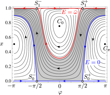
Figure 1: Contours of (19) and fixed points of (17-18) for a triad with $\overline{\omega}=-0.76$, and $\kappa=1.2$. The phase space is separated in regions with bounded (white) and unbounded motions (gray) in $\varphi$. The separatrices in blue and red contain solutions with infinite period and delimit the regions with finite period solutions.

In Fig. 1, we divided the phase space $\varphi-x$, in three sub-domains depending on the type of behavior of $\varphi$. Two regions with bounded oscillations in $\varphi$ (in white), where $E\char 60\relax\overline{\omega}$ and $E>0$, separated by a region with unbounded evolution of $\varphi$ (in gray), where $\overline{\omega}\char 60\relax E\char 60\relax 0$. The evolution of $x$ is always bounded and periodic, which is expected due to $r_{3}\char 60\relax I_{\min}$, and because of the dimension of the space, except for the infinite time orbits in the separatrices that only arrive (or depart) asymptotically to (from) the saddle points. Expectedly, the frequency of the solutions will go to zero at the separatrices and have finite values otherwise, tending to the linear frequencies near the centers $C_{0},C_{\pi}$ for close small amplitude oscillations.

To summarize, in this particular situation, for $E\char 60\relax\overline{\omega}\char 60\relax 0$, the amplitude of the third wave $r_{3}\propto x$ oscillates around a large value, and its phase oscillates about $\varphi=0$. As we increase the energy, to $\overline{\omega}\char 60\relax E\char 60\relax 0$, the fluctuations in the wave amplitude grow, but now occur about an intermediate value, and the mismatch phase $\varphi$, moves counterclockwise and unbounded. Finally, if we increase the energy to $E>0$, the fluctuations in the amplitude decrease and occur about an even lower value, while the mismatch phase gets confined again, but oscillates about $\varphi=\pi$. As will be illustrated now, this analysis reverses when $\overline{\omega}>0$.

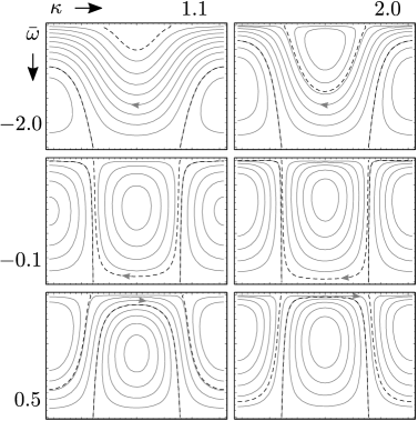
Figure 2: Phase space dependence on the control parameters. Large magnitudes of $\overline{\omega}$ increase the unbounded solutions, while large values of $\kappa$ reduce the amount of bounded solutions.

In Fig. 2 we depict in few instances of phase space for different parameters $\overline{\omega}$ and $\kappa$. The centers $C_{0}$ and $C_{\pi}$, $x$-coordinate interchange as $\overline{\omega}$ goes from negative to positive, and the separatrices flip the bounded region when the phase mismatch flips direction as well. Also, since the unbounded motion occurs between $E=\overline{\omega}$ and $E=0$, larger magnitudes of $\overline{\omega}$ lead to larger regions of unbounded motion. Conversely, increases in $\kappa$, push the separatrices to each other, reducing the size of the rotation region.

III.1 Inherent modal drift

In this work, we are interested in the development of atmospheric patterns and their persistence in relation to atmospheric blockings. As mentioned before, the contribution to the flow pattern from a mode $\alpha=(m,n)$ has the form

$$\psi_{\alpha}\propto r_{\alpha}(t)P_{n}^{m}(\cos\theta)\cos(m_{i}\phi+\varphi_{i}(t)),$$

where the modal phase $\varphi_{i}(t)$, introduces a time-dependent offset in the zonal direction for the mode contribution to the global flow pattern. In the context of atmospheric blocking, we can expect that the relevant mode $\psi_{3}$, sustains a relatively large amplitude $r_{3}$ for a long time, and its phase becomes stagnant or oscillates about the blocking longitude $\varphi_{b}$, which might be correlated to the topography phase $\varphi_{h}$, that already sets the zero of the mode phases in (9).

An interesting candidate for the blocking states are those orbits close to the high amplitude center at mismatch value $\varphi=0$ (available for $\overline{\omega}\char 60\relax 0$), where the amplitude of $r_{3}$ is stably large and $\varphi(t)$ oscillates about zero. This, however does not imply that the individual phases $\varphi_{i}(t)$ are oscillating too, but only their mismatch. In the following we address the conditions under which the relevant mode $\varphi_{3}$ tends to oscillate about zero as well.

Consider the rescaled equation for the phase of the topography mode $\varphi_{3}$

$$\begin{array}[]{lll}\frac{d\varphi_{3}}{d\tau}&=&\overline{\omega}_{3}-A(x)\cos\varphi,\end{array}$$

where $A(x)=(1-x^{2})^{1/2}(\kappa^{2}-x^{2})^{1/2}/x$,  $\overline{\omega}_{3}=\omega_{3}/I_{\min}$. Now, we consider a periodic solution near the fixed point $C_{0}=(0,x_{0})$, which can be approximated in the linear region by

$$x(\tau) \approx x_{0}+a_{x}\cos(\omega_{0}\tau)$$

$$\varphi(\tau) \approx a_{\varphi}\sin(\omega_{0}\tau)$$

where $\omega_{0}$ is the linear frequency at the fixed point $C_{0}$, and the fluctuation amplitudes $a_{x}$, $a_{\varphi}$, satisfy $|a_{x}|\ll x_{0}$, and $|a_{\varphi}|\ll 1$. To a second order, the evolution of the phase velocity along the linear solution is

$$\frac{d\varphi_{3}}{d\tau} \approx \overline{\omega}_{3}-A(x_{0})-a_{x}A^{\prime}(x_{0})\cos(\omega_{0}\tau)$$

$$-\frac{a_{x}^{2}}{2}A^{\prime\prime}(x_{0})\cos^{2}(\omega_{0}\tau)+a^{2}_{\varphi}A(x_{0})\sin^{2}(\omega_{0}\tau),$$

and the drift velocity of the third phase is the average of $\dot{\varphi_{3}}$ taken along the orbit

$$u_{3}=\frac{1}{T}\int_{0}^{T}\frac{d\varphi_{3}}{d\tau}d\tau,$$

which leads to the simple form

$$u_{3}=\overline{\omega}_{3}-A_{0}+(a_{\varphi}^{2}A_{0}-a_{x}^{2}A_{0}^{\prime\prime})/4,$$ (20)

giving the actual drift velocity of a wave pattern in the zonal direction as a function of the amplitude of the phase fluctuation $a_{\varphi}$ and the coordinate $x_{0}$, of the fixed point $C_{0}$ in phase space $\varphi-x$.

In principle, the zonal drift of $\psi_{3}$ (20), can vanish for a particular choice of system parameters, and at one single particular solution in phase space, e.g., if we take an oscillation in $x-\varphi$ for which $\overline{\omega}_{3}=A_{0}-(a_{\varphi}^{2}A_{0}-a_{x}^{2}A_{0}^{\prime\prime})/4$, so that the corresponding level set in $\varphi-x$ becomes the limit between positive and negative drifting evolution for $\varphi_{3}$.

In Fig. 3, we show a particular triplet that supports zero-drift solutions for $\varphi_{3}$, corresponding parameters are $\overline{\omega}=-1.18$, $\kappa=1.66$, and $x_{0}=0.8$. As described above, the zero drift solution occurs at a single level set in phase space, and other solutions exhibit positive or negative drift depending on whether they are inside or outside such contour.

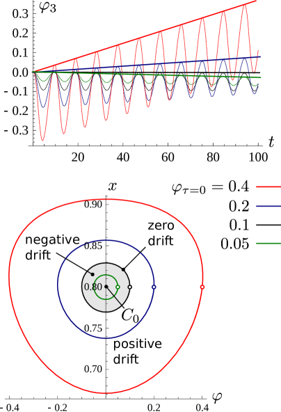
Figure 3: Dynamics of the third phase $\varphi_{3}$, for a triad supporting a zero-drift solution (black waveform and contour) at a stationary, high-amplitude of the third wave. At the stagnant amplitude $x_{0}$, the phase may drift in a positive or negative direction, depending on the initial mismatch $\varphi_{0}$. The zero drift solution starting at $(\varphi_{0},x_{0})=(0.8,0.2)$ is in a closed contour in $\varphi-x$, about the elliptic point $C_{0}$, and separates positive from negative drift solutions for the third wave.

Since zero-drift solutions of (20), have zero measure in phase space, it is clear that the mode locking required for the atmospheric blocking is not a statistically representative in the space of solutions, and consequently, is not a feature on the dynamics of a single triad, and, in general, all modes will drift with finite velocity in the real space. In the following, we will show that mode locking is a more general feature of the dynamics when a topography mode interacts with the triad at particular system parameters, i.e. there is a nonzero measure region in phase space where this phenomenon occurs.

IV single triad with topography

Now that we identified the fundamental parameters of a single triad without topography, we can characterize better the effects of the interaction with a single topography mode congruent with the third wave pattern. Before rewriting the original system (9) in polar form, it can be seen that $I_{1}$ and $I_{2}$ as defined in (15, 16) are no longer constants of motion, but we can use them to derive a new invariant of the form

$$M^{2}=\pm[\varepsilon_{2}(|z_{1}|^{2}+|z_{3}|^{2})-\varepsilon_{1}(|z_{2}|^{2}+|z_{3}|^{2})],$$ (21)

where the sign is chosen in such a way that $M>0$. Provided that $M$ is a constant, the largest Manley-Rowe quantity (mult. by the corresponding $\varepsilon$), will be always be so, maintaining its distance to the other quantity. In general, we can put $r_{3}$ in terms of $r_{1},r_{2}$ using (21) and the system parameters, then, the original system (9) can be recasted in polar form to obtain the four-dimensional system

$$\dot{r_{1}} = r_{2}r_{3}(r_{1},r_{2})\sin\varphi+\varepsilon_{1}r_{2}\sin(\varphi-\varphi_{3}),$$

$$\dot{r_{2}} = r_{1}r_{3}(r_{1},r_{2})\sin\varphi+\varepsilon_{2}r_{1}\sin(\varphi-\varphi_{3}),$$

$$\dot{\varphi} = \omega+\left[\left(\frac{r_{2}}{r_{1}}+\frac{r_{1}}{r_{2}}\right)r_{3}(r_{1},r_{2})-\frac{r_{1}r_{2}}{r_{3}(r_{1},r_{2})}\right]\cos\varphi$$

$$+\left(\varepsilon_{1}\frac{r_{2}}{r_{1}}+\varepsilon_{2}\frac{r_{1}}{r_{2}}\right)\cos(\varphi-\varphi_{3}),$$

$$\dot{\varphi}_{3} = \omega_{3}-\frac{r_{1}r_{2}}{r_{3}(r_{1},r_{2})}\cos\varphi,$$

where the function $r_{3}$, takes an appropriate form, for instance $r_{3}(r_{1},r_{2})=[(M^{2}+\varepsilon_{1}r_{2}^{2}-\varepsilon_{2}r_{1}^{2})/(\varepsilon_{2}-\varepsilon_{1})]^{1/2}.$ In the case without topography the evolution was entirely determined by the initial phase mismatch $\varphi=\varphi_{3}-\varphi_{2}-\varphi_{1}$, and the modal amplitudes, but in this case the initial phase of $\varphi_{3}$, must be specified as well.

To understand the effect of the topography in the third phase, notice that the perturbation does not affect the equation for $\dot{\varphi_{3}}$ directly but only trough its cumulative effects in $r_{1}(t)$ and $r_{2}(t)$, which are no longer specified uniquely by the value of $r_{3}$ and the constants of motion. As before, consider the average of the equation for $\dot{\varphi}_{3}$ along a trajectory close to $C_{0}$.

$$u_{3}=\omega_{3}-\frac{1}{T}\int_{0}^{T}\frac{r_{1}(t)r_{2}(t)}{r_{3}(r_{1}(t),r_{2}(t))}\cos\varphi(t)\operatorname{dt},$$

where $T$ is the period of the corresponding unperturbed orbit around $C_{0}$. Provided that $r_{1}(t)$, $r_{2}(t)$ and $\varphi(t)$ are no longer exactly periodic, the resulting drift velocity for one cycle will differ slightly from the next, and the drift velocity becomes a function of time.

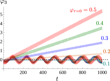
Figure 4: Evolution of the third phase for a single triad (dotted) and a triad with topography (continuous), for the same initial value of the amplitudes different values of the initial mismatch $\varphi(\tau=0).$

In Fig. 4 we show the results of the numerical integration of the equations of motion for one triad with $\overline{\omega}=-1.0,\kappa=1.34$, with and without topography for different initial conditions in $r_{3}-\varphi$. For this choice of parameters the system contains an elliptic fixed point with large amplitude, $x_{0}=r_{3,0}/I_{\min}=0.8$, around which we will study the motion with perturbation amplitudes of $\varepsilon_{1}=0.01,\varepsilon_{2}=0.0175$. As mentioned above the drift velocity in the unperturbed case is constant and the phase of the third mode in general oscillates while drifting away. This occurs even when the initial condition in phase space corresponds to bounded solutions of the mismatch phase $\varphi$ (which is here the case). On the other hand, when we introduce a topography mode congruent with the wave $\psi_{3}$, for the same initial conditions, we obtain a bounded periodic phase drift for $\varphi_{3}$ about its initial value, in other words, the topography effectively locks its corresponding Rossby wave spatially for a finite region of phase space, i.e. in contrast with the unperturbed triad the perturbed solutions exhibiting bounded drifts have finite measure in phase space, and consequently finite probability when sorting initial configurations.

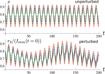
Figure 5: Comparison between the corresponding third mode amplitudes for different initial mismatches (same as Fig. 4) in the perturbed and unperturbed situations.

A complementary important feature of the perturbed motion is that it does not affect importantly the amplitude of the relevant wave, but only modulates it slightly in time. With this, we combine the two required features for simplified atmospheric blocking, a bounded drift of the third Rossby wave with a sustained large amplitude.

V conclusions

It this work we have shown that individual triads of the barotropic quasi-geostrophic model present unbounded phase drifts on each mode, implying that the underlying flow pattern of each wave oscillates about a rotating phase in the real space. The drift motion is even present when the triad mismatch phase performs bounded oscillations in phase space at high amplitudes of a relevant mode. Particular solutions without drift do exist, but these have zero measure in phase space. Not surprisingly, this implies that a single triad is unable to represent the meridional persistence of atmospheric blocking, one its most basic features. This scenario changes drastically by the introduction of a single topography mode consistent with one wave in the Rossby-Hawritz triad. The topography here acts as a small perturbation on the Hamiltonian system leading to periodic changes in the drift velocity, resulting in the non-linear phase capture of the corresponding mode. This generates a finite volume of solutions in phase space without net phase drift for the mode consistent with the topography, i.e. persistent patterns have a finite probability when initial conditions are randomly selected in phase space. Fortunately, such important changes in the phase dynamics do not affect drastically the characteristic large amplitude of the mode corresponding to the topographic pattern, and, consequently, the topography-related mode can be large while its phase is bounded meridionally in real space. The results obtained in this work are very general, as the mechanisms mentioned here were not obtained for particular modal structures, numerical examples were used for illustrative purposes, but they do not restrict our analysis, which is in fact, based in a rescaled dimensionless dynamical system encompasing an infinite family of triads. With this we are implying that the non-linear phase capture is a common mechanism triggered by topography (or any inhomogeneity in the atmospheric layer), and it leads to dynamical features consistent with atmospheric blockings. The emergence of such states or their duration might involve the interaction with other triads, and will be investigated in a future paper, but the prescence of persistent patterns in the elementary triads is already expected from this reductionist treatment.

VI Appendix

VI.1 Derivation of the quasi-geostrophic model

In general, the conservation of the potential vorticity in an incompressible two-dimensional flow in a rotating frame with angular velocity $\Omega$ is given by

$$D_{t}\left(\frac{\zeta+f}{H}\right)=0,$$ (22)

where $\zeta=\hat{n}\cdot\nabla\times\vec{u}$ is the relative vorticity, with $\hat{n}$ the normal to the planet surface, $f=2\Omega\cos\theta$ the planetary vorticity, and $H(\theta,\phi,t)$ the fluid depth at the latitude $\theta$, longitude $\phi$ and time $t$. The material derivative is defined in terms of the relative velocity in the rotating frame $D_{t}=\partial/\partial t+\vec{u}\cdot\nabla$, so that mass conservation reads

$$D_{t}H=-H\nabla\cdot\vec{u}$$ (23)

which inserted in (22) leads to

$$D_{t}(\zeta+f)+(\zeta+f)\nabla\cdot\vec{u}=0,$$ (24)

which can be recasted in conservation form as

$$\partial_{t}\zeta+\nabla\cdot[(\zeta+f)\vec{u}]=0,$$ (25)

where it becomes clear that the potential vorticity is carried by the velocity flow.

Now, in order to obtain a useful yet simple model of the atmosphere we consider the particular situation in which the dept $H$ is not changing in time, so that the flow $H\vec{u}$ becomes incompressible, and can be written in terms of a suitable stream function $\xi$ in the form

$$H\vec{u}=\hat{n}\times\nabla\xi.$$ (26)

Decomposing the depth in a large mean $\bar{H}$ and a small fluctuation $\tilde{H}$, and dividing both sides of (26) by the mean depth $\bar{H}$, we can write the non-solenoidal velocity field as

$$\vec{u}=\frac{\hat{n}\times\nabla\psi}{(1+\eta)},$$ (27)

where $\eta=\tilde{H}(\theta,\phi)/\bar{H}$, and $\psi=\xi/\bar{H}$. Replacing this form of the velocity in (25) we obtain a new form of the conservation of the absolute vorticity

$$\frac{\partial\zeta}{\partial t}+J\left(\psi,\frac{\zeta+f}{1+\eta}\right)=0,$$ (28)

where $J(f_{1},f_{2})=\hat{n}\cdot(\nabla f_{1}\times\nabla f_{2})$. This equation, now in terms of scalar fields alone requires an additional relation between the stream $\psi$ and the relative vorticity $\zeta$, given by

$$\zeta=\frac{\nabla^{2}\psi}{1+\eta}-\frac{\nabla\eta\cdot\nabla\psi}{(1+\eta)^{2}},$$ (29)

which, formally, allow us to determine the evolution of the stream, provided that we know the static relative fluctuation $\eta$. The fluctuation is due to both the topography and the free surface, but here we will refer to it as the topography.

VI.1.1 Perturbative expansion and hybrid model

In the limit without topography $\eta\rightarrow 0$, the velocity field becomes solenoidal and (28) becomes the regular non-linear form of the barotropic vorticity (BV) equation. This indicates a functional dependence between the stream $\psi$ and the topography $\eta$, which can be weighted by a tunable parameter $\varepsilon$, then perform a perturbative expansion of the form

$$\psi=\psi_{0}+\varepsilon\psi_{1}+\cdots,$$

The leading orders of (29) are

$$\zeta_{0}+\varepsilon\zeta_{1}=\nabla^{2}\psi_{0}+\varepsilon(\nabla^{2}\psi_{1}-\eta\nabla^{2}\psi_{0}-\nabla\eta\cdot\nabla\psi_{0}),$$ (30)

which replaced in (28) leads to

$$\frac{\partial}{\partial t}(\zeta_{0}+\varepsilon\zeta_{1})+J[\psi_{0}+\varepsilon\psi_{1},(\zeta_{0}+\varepsilon\zeta_{1}+f)(1-\varepsilon\eta)]=0,$$ (31)

where $\zeta_{0}=\nabla^{2}\psi_{0}$, and $\zeta_{1}=\nabla^{2}\psi_{1}-\eta\nabla^{2}\psi_{0}-\nabla\eta\cdot\nabla\psi_{0}$, are the zero and first order vorticity. At this point, if we perform a regular separation in powers of $\varepsilon$, we recover the regular barotropic vorticity equation at order zero and get a complicated expression for the first order, which includes the topography. Instead of proceeding in this fashion, we consider the influence of the topography on the zeroth order atmospheric patterns and collect the remaining terms in an auxiliary equation indented to correct the stream to a first order:

$$\frac{\partial\zeta_{0}}{\partial t}+J(\psi_{0},\zeta_{0}+f-\eta f) = 0,$$ (32)

$$\frac{\partial\zeta_{1}}{\partial t}+J(\psi_{1},\zeta_{0}+f)+J(\psi_{0},\zeta_{1}-\eta\zeta_{0}) = 0,$$ (33)

Equation (32) resembles the usual BV equation but now includes a topographic forcing weighted by the Coriolis parameter $h=\eta f=2\Omega\tilde{H}\cos\theta/\bar{H}$. Dropping the indices we obtain a hybrid model between zero and one used along the text.

$$\frac{\partial\zeta}{\partial t}+J(\psi,\zeta+f-h),$$ (34)

where $\zeta=\nabla^{2}\psi$, and the velocity is non-solenoidal because of the topography correction.

$$\vec{u}=(1-h/f)\hat{n}\times\nabla\psi.$$ (35)

VI.2 Reduced dynamical system and modal interaction

In general, by introduzing the stream expansion (3), and the topography decomposition (4), in the barotropic quasi-geostrophic equation (2). And using the orthogonality of the spherical harmonics, it can be shown that the dynamics of the amplitudes is given by

$$k_{\gamma}\dot{a}_{\gamma}=im_{\gamma}a_{\gamma}+i\sum_{\alpha,\beta}K_{\gamma\beta\alpha}[\lambda k_{\beta}a_{\alpha}a_{\beta}+\varepsilon a_{\alpha}h_{\beta}],$$ (36)

where $(\alpha,\beta,\gamma)$ are collective indices of the form $\gamma=(m_{\gamma},n_{\gamma})$, and $k_{\gamma}=n_{\gamma}(n_{\gamma}+1)$. The products between amplitudes are a consequence of the nonlinearity of the Jacobian function, and are weighted by the interaction coefficients $K$ defined by

$$K_{\gamma\beta\alpha}=\int_{-1}^{1}P_{\gamma}\left(m_{\beta}P_{\beta}\frac{dP_{\alpha}}{dz}-m_{\alpha}P_{\alpha}\frac{dP_{\beta}}{dz}\right)dz,$$ (37)

where $P_{\gamma}(z)=P_{n}^{m}(\cos\theta)$ are the associated Legendre polynomial, and it can be shown that the $K$’s vanish, unless the following conditions are satisfied.

$$m_{\alpha}+m_{\beta} = m_{\gamma},$$

$$m^{2}_{\alpha}+m^{2}_{\beta} \neq 0,$$

$$n_{\alpha}n_{\beta}n_{\gamma} \neq 0,$$

$$n_{\alpha} \neq n_{\beta},$$

$$n_{\alpha}+n_{\beta}+n_{\gamma} \operatorname{is} \operatorname{odd},$$

$$(n_{\alpha}-|m_{a}|)^{2}+(n_{\beta}-|m_{\beta}|)^{2} \neq 0,$$

$$|n_{\alpha}-n_{\beta}|\char 60\relax n_{\gamma} \char 60\relax n_{\alpha}+n_{\beta},$$

$$\beta\neq\bar{\gamma} \operatorname{and} \alpha\neq\bar{\gamma},$$

where $\bar{\gamma}=(-m_{\gamma},n_{\gamma})$, for $\gamma=(m_{\gamma},n_{\gamma})$.

$$in_{1}(n_{1}+1)\dot{a}_{1} = -m_{1}a_{1}+\lambda K\mu_{32}a_{2}^{\ast}a_{3}$$

$$-\varepsilon K(h_{2}^{\ast}a_{3}-h_{3}a_{2}^{\ast}),$$

$$in_{2}(n_{2}+1)\dot{a}_{2} = -m_{2}a_{2}+\lambda K\mu_{13}a_{1}^{\ast}a_{3}$$

$$+\varepsilon K(h_{1}^{\ast}a_{3}-h_{3}a_{1}^{\ast}),$$

$$in_{3}(n_{3}+1)\dot{a}_{3} = -m_{3}a_{3}+\lambda K\mu_{12}a_{1}a_{2}$$

$$-\varepsilon K(h_{2}a_{1}-h_{1}a_{2}).$$

VI.3 Fixed points of a single triad

In the following we classify the fixed points and stability of the single triad two-dimensional system (17-18). By requiring $dx/d\tau=0$, and recalling that $x\leqslant 1$, and $\kappa\geqslant 1$ we obtain the conditions

$$x_{1}=1,\quad\varphi_{2}=0,\quad\varphi_{3}=\pi,$$ (38)

Now we examine these conditions respect to the equation for the evolution in $\varphi$

$$\frac{d\varphi}{d\tau} = \overline{\omega}+\left(\frac{x}{\kappa^{2}-x^{2}}+\frac{x}{1-x^{2}}-\frac{1}{x}\right)\times$$

$$(1-x^{2})^{1/2}(\kappa^{2}-x^{2})^{1/2}\cos\varphi$$

which, when $x\rightarrow x_{1}$=1 takes the form

$$\frac{d\varphi}{d\tau} \rightarrow \overline{\omega}+\frac{(\kappa^{2}-1)^{1/2}}{(1-x^{2})^{1/2}}\cos\varphi,$$

so that as $x\rightarrow 1$ the motion in phase space becomes mostly horizontal, but because of $\cos\varphi$, the direction of $d\varphi/d\tau$ reverses at $\varphi\pm\pi/2$, regardless of the finite offset caused by $\overline{\omega}$, then, we have two fixed points

$$x_{1}=1,\quad\varphi_{1}^{+}=\pi/2,\quad\varphi_{1}^{-}=-\pi/2.$$ (39)

Notice also, that $d\varphi/d\tau$ also diverges as $x\rightarrow 0$, which means that, even in $dx/d\tau$ is finite, the flow in phase space becomes horizontal, but, by the previous argument, reverses at $\varphi\pm\pi/2$, leading to a couple of new fixed points

$$x_{4}=0,\quad\varphi_{4}^{+}=\pi/2,\quad\varphi_{4}^{-}=-\pi/2.$$

For the remaining fixed points we insert $\varphi_{2}$ and $\varphi_{3}$ in $d\varphi/d\tau=0$, to obtain

$$\overline{\omega}x\sqrt{(1-x^{2})(\kappa^{2}-x^{2})}\pm[2(1+\kappa^{2})x^{2}-3x^{4}-\kappa^{2}]=0$$ (40)

which can be written as quartic polynomial equation in $x^{2}$, and can be solved using computational algebra, but such solution is extensive and has little value for phenomenological interpretation. However, we can guarantee that such solution exist for both $\varphi_{2}$ and $\varphi_{3}$. To see this, note that the l.h.s. function in (40) can be written as

$$f_{\operatorname{lhs}}(x)=\overline{\omega}f_{1}(x)\pm f_{2}(x),$$

where $f_{1}(0)=f_{1}(1)=0$, and $f_{2}(0)=-\kappa^{2}$, $f_{2}(1)=\kappa^{2}-1$. Provided that $f_{2}(0)\char 60\relax 0$ and $f_{2}(1)>0$, the function $f_{\operatorname{lhs}}$ changes sign between $x=0$ and $x=1$,  regardless of the sign of $\overline{\omega}$. Given that $f_{\operatorname{lhs}}(x)$ has no singularities it follows that it must vanish at least one time in $0\char 60\relax x\char 60\relax 1$. With this we guarantee that there is at least one pair of fixed point solutions

$$\varphi_{2}=0\quad,0\char 60\relax x_{2}\char 60\relax 1,\quad\varphi_{3}=\pi,\quad 0\char 60\relax x_{3}\char 60\relax 1,$$

with further analysis we can make the intervals narrower, but here we are only interested in the existence of such fixed points. To summarize we have

$$S_{1}^{\pm}:\quad(\varphi_{1}^{\pm},x_{1}) = (\pm\pi/2,1)\rightarrow\operatorname{hyperbolic},$$

$$S_{0}^{\pm}:\quad(\varphi_{1}^{\pm},x_{4}) = (\pm\pi/2,0)\rightarrow\operatorname{hyperbolic},$$

$$C_{0}:\quad(\varphi_{2},x_{2}) = (0,0\char 60\relax x_{2}\char 60\relax 1)\rightarrow\operatorname{Elliptic},$$

$$C_{\pi}:\quad(\varphi_{3},x_{3}) = (\pi,0\char 60\relax x_{2}\char 60\relax 1)\rightarrow\operatorname{Elliptic}.$$

The classification of these equilibria was made through the discriminant of the Jacobian matrix, and it wont be explicited here.

References

- (1) F. P. Bretherton and D. B. Haidvogel. Two-dimensional turbulence above topography. Journal of Fluid Mechanics, 78(1):129, 1976.
- (2) E. de Lima Nascimento and T. Ambrizzi. The influence of atmospheric blocking on the rossby wave propagation in southern hemisphere winter flows. Journal of the Meteorological Society of Japan, Ser. II 80.2:139, 2002.
- (3) T. M. Hamill and G. N. Kiladis. Skill of the mjo and northern hemisphere blocking in gefs medium range reforecasts. Monthly Weather Review, 142(2):868, 2014.
- (4) S. Pfahl and H. Wernli. Quantifying the relevance of atmospheric blocking for co-located temperature extremes in the northern hemisphere on (sub-) daily time scales. Geophysical Research Letters, 39(12), 2012.
- (5) J. A. Renwick. Enso-related variability in the frequency of south pacific blocking. Monthly Weather Review, 126(12):3117, 1998.
- (6) A. A. Scaife, D. Copsey, C. Gordon, C. Harris, T. Hinton, S. Keeley, A. O’Neill, M. Roberts, and K. Williams. Improved atlantic winter blocking in a climate model. Geophysical Research Letters, 38(23), 2011.
- (7) J. Sillmann, M. Croci-Maspoli, M. Kallache, and R. W. Katz. Extreme cold winter temperatures in europe under the influence of north atlantic atmospheric blocking. Journal of Climate, 24(22):5899, 2011.