Error analysis of an L2-type method on graded meshes for a fractional-order parabolic problem

Abstract.

An initial-boundary value problem with a Caputo time derivative of fractional order $\alpha\in(0,1)$ is considered, solutions of which typically exhibit a singular behaviour at an initial time. An L2-type discrete fractional-derivative operator of order $3-\alpha$ is considered on nonuniform temporal meshes. Sufficient conditions for the inverse-monotonicity of this operator are established, which yields sharp pointwise-in-time error bounds on quasi-graded temporal meshes with arbitrary degree of grading. In particular, those results imply that milder (compared to the optimal) grading yields optimal convergence rates in positive time. Semi-discretizations in time and full discretizations are addressed. The theoretical findings are illustrated by numerical experiments.

1. Introduction

The Caputo time derivative of fractional order $\alpha\in(0,1)$, which will be denoted by $D_{t}^{\alpha}$, is defined [3] by

(1.1) $$D_{t}^{\alpha}u(\cdot,t):=\frac{1}{\Gamma(1-\alpha)}\int_{0}^{t}(t-s)^{-\alpha}\,\partial_{s}u(\cdot,s)\,ds\qquad\text{for }\ 0<t\leq T,$$

where $\Gamma(\cdot)$ is the Gamma function, and $\partial_{s}$ denotes the partial derivative in $s$.

The paper is devoted to the analysis of an L2-type discrete fractional-derivative operator for $D_{t}^{\alpha}$ from [10], based on piecewise-quadratic Lagrange interpolants. In [10], this operator is analysed on uniform temporal meshes, and the optimal convergence order $3-\alpha$ in time is established under strong regularity assumptions on the exact solution. (Similar L2-type discretizations of order $3-\alpha$ on uniform temporal meshes were considered, e.g., in articles [4, 13], the latter giving optimal error bounds in positive time taking into account more realistic low regularity of the exact solution.)

The purpose of this paper is consider this discrete fractional-derivative operator on more general quasi-graded temporal meshes. For this, we employ the framework from the recent paper [9] (which builds on the analysis of [8], and, to some degree, [2]). This approach is based on barrier functions for derivation of subtle stability properties, and allows, in a relatively simple way, to get sharp pointwise-in-time error bounds on quasi-graded temporal meshes with arbitrary degree of grading.

• However, compared to the two methods considered in [9], the L1 scheme and the Alikhanov L2-1_σ scheme, now we have a significantly more challenging case, as the considered discrete fractional-derivative operator is not associated with an M-matrix. So our main challenge in this paper will be to establish the inverse-monotonicity of the discrete operator on nonuniform meshes.

• For the same reason, the generalization of our error analysis to the parabolic case also becomes substantially more challenging.

Note that the inverse-monotonicity on uniform temporal meshes was established in [10]. However, the evaluations in the latter article are quite intricate, so it is not clear whether they can be generalized to more general meshes. We take a very different route and employ a non-standard set of basis functions (see Fig. 1), which very naturally leads to a representation of the discrete operator as a product of two M-matrices. To be more precise, the discrete version $\delta_{t}^{\alpha}$ of the Caputo fractional-derivative operator $D_{t}^{\alpha}$ will be represented in the form

(1.2a) $$\delta_{t}^{\alpha}U^{m}=\sum_{j=0}^{m}\kappa_{m,j}V^{j}\;\;\forall\,m\geq 1,\quad V^{j}:=\frac{U^{j}-\beta_{j}U^{j-1}}{1-\beta_{j}}\;\;\forall\,j\geq 1,\quad V^{0}:=U^{0},$$

where $$\beta_{j}\in[0,1) \{\beta_{j}\}$$. Then relatively simple sufficient conditions will be formulated for choosing a set such that

(1.2b) $$\kappa_{m,m}>0\;\;\mbox{and}\;\;\sum_{j=0}^{m}\kappa_{m,j}=0\;\;\forall\,m\geq 1,\quad\kappa_{m,j}\leq 0\;\;\forall\,0\leq j<m\leq M.$$

As the representation (1.2) immediately implies that $\delta_{t}^{\alpha}$ is associated with an inverse-monotone matrix (see Remark 2.1), the required stability properties of the discrete fractional-derivative operator follow, which enables us to employ the error analysis framework from [9].

This error analysis will be applied for the fractional-order parabolic problem

(1.3) $$\begin{array}[]{l}D_{t}^{\alpha}u+{\mathcal{L}}u=f(x,t)\quad\mbox{for}\;\;(x,t)\in\Omega\times(0,T],\\[5.69046pt] u(x,t)=0\quad\mbox{for}\;\;(x,t)\in\partial\Omega\times(0,T],\qquad u(x,0)=u_{0}(x)\quad\mbox{for}\;\;x\in\Omega.\end{array}$$

This problem is posed in a bounded Lipschitz domain $\Omega\subset\mathbb{R}^{d}$ (where $d\in\{1,2,3\}$). The spatial operator ${\mathcal{L}}$ here is a linear second-order elliptic operator defined by

(1.4) $${\mathcal{L}}u:=\sum_{k=1}^{d}\bigl{\{}-\partial_{x_{k}}\!(a_{k}(x)\,\partial_{x_{k}}\!u)\bigr{\}}+c(x)\,u,$$

with sufficiently smooth coefficients $\{a_{k}\}$ and $c$ in $C(\bar{\Omega})$, for which we assume that $a_{k}>0$ and $c\geq 0$ in $\bar{\Omega}$.

The L2-type fractional-derivative operator that we consider, denoted $\delta_{t}^{\alpha}$, is defined as follows. On the temporal mesh $0=t_{0}<t_{1}<\ldots<t_{M}=T$, $\forall\,m=1,\ldots,M$ let

(1.5a) $$\delta_{t}^{\alpha}U^{m}:=D^{\alpha}_{t}(\Pi^{m}U)(t_{m}),\quad\quad\Pi^{m}:=\left\{\begin{array}[]{cll}\Pi_{1,1}&\mbox{on~{}}(0,t_{1})&\mbox{for~{}}m=1,\\ \Pi_{2,j}&\mbox{on~{}}(t_{j-1},t_{j})&\mbox{for~{}}1\leq j<m,\\ \Pi_{2,j-1}&\mbox{on~{}}(t_{j-1},t_{j})&\mbox{for~{}}j=m>1,\\ \end{array}\right.$$

where $$\Pi_{1,j} \Pi_{2,j}$$ and are the standard linear and quadratic Lagrange interpolation operators with the following interpolation points:

(1.5b) $$\Pi_{1,j}\;:\;\{t_{j-1},t_{j}\},\qquad\qquad\Pi_{2,j}\;:\;\{t_{j-1},t_{j},t_{j+1}\}.$$

Similarly to [12, 8, 2], our main interest will be in graded temporal meshes as they offer an efficient way of computing reliable numerical approximations of solutions singular at $t=0$, which is typical for (1.3). It should be noted that these three papers are concerned with global-in-time error bounds on graded meshes. There is also a lot of interest in the literature in optimal error bounds in positive time on uniform meshes; see, e.g. [5, 7, 8]. By contrast, here, following the recent paper [9], pointwise-in-time error bounds will be obtained, while an arbitrary degree of mesh grading (with uniform meshes included as a particular case) is allowed. In particular, our results imply that milder (compared to the optimal) grading yields optimal convergence rates in positive time; see Remarks 4.2 and 4.3.

Throughout the paper, it is assumed that there exists a unique solution of this problem such that $\|\partial_{t}^{l}u(\cdot,t)\|_{L_{2}(\Omega)}\lesssim 1+t^{\alpha-l}$ for $l\leq 3$. This is a realistic assumption, satisfied by typical solutions of problem (1.3), in contrast to stronger assumptions of type $\|\partial^{l}u(\cdot,t)\|_{L_{2}(\Omega)}\lesssim 1$ frequently made in the literature (see, e.g., references in [6, Table 1.1]). Indeed, [11, Theorem 2.1] shows that if a solution $u$ of (1.3) is less singular than we assume, then the initial condition $u_{0}$ is uniquely defined by the other data of the problem, which is clearly too restrictive. At the same time, our results can be easily applied to the case of $u$ having no singularities or exhibiting a somewhat different singular behaviour at $t=0$ (see Remark 4.6).

Outline. Sufficient conditions for inverse-monotonicity of the discrete fractional-derivative operator are established in §2, which enables us to establish its stability properties on quasi-graded meshes in §3. Error analysis for a simplest example without spatial derivatives is given in §4, while semi-discretizations in time and full discretizations for the parabolic case are addressed in §5. Finally, our theoretical findings are illustrated by numerical experiments in §6.

Notation. We write $a\simeq b$ when $a\lesssim b$ and $a\gtrsim b$, and $a\lesssim b$ when $a\leq Cb$ with a generic positive constant $C$ depending on $\Omega$, $T$, $u_{0}$ and $f$, but not on the total numbers of degrees of freedom in space or time. Also, for $k\geq 0$, we shall use the standard norms in the space $L_{2}(\Omega)$ and the related Sobolev spaces $W_{2}^{k}(\Omega)$, while $H^{1}_{0}(\Omega)$ is the standard space of functions in $W_{2}^{1}(\Omega)$ vanishing on $\partial\Omega$.

2. Inverse-monotonicity of the discrete fractional-derivative operator

In this section we shall establish sufficient conditions on the temporal mesh $\{t_{j}\}_{j=0}^{M}$ for the inverse-monotonicity of the discrete fractional-derivative operator $\delta_{t}^{\alpha}$. The latter is understood in the sense that the matrix associated with $\delta_{t}^{\alpha}$ is inverse-monotone, i.e. all elements of the inverse of this matrix are non-negative.

The following notation for the temporal mesh will be used throughout the paper:

(2.1) $$\tau_{j}:=t_{j}-t_{j-1},\quad{\tilde{\tau}}_{j}:={\textstyle\frac{1}{2}}(\tau_{j-1}+\tau_{j}),\quad\rho_{j}:=\frac{\tau_{j}}{\tau_{j-1}},\quad\sigma_{j}:=\frac{\tau_{j}-\tau_{j-1}}{\tau_{j}+\tau_{j-1}}=1-\frac{2}{1+\rho_{j}}.$$

2.1. Matrix product representation for the discrete fractional-derivative operator

Our first task will be to find a representation for $\delta_{t}^{\alpha}$ in the form (1.2a), where the set of real numbers $\{\beta_{j}\}_{j=0}^{M}$, with $\beta_{j}\in[0,1)$ and $\beta_{0}=0$, is such that (1.2b) is satisfied.

Remark 2.1 (Inverse monotonicity).

Set $F^{m}:=\delta_{t}^{\alpha}U^{m}$ for $m=1,\ldots,M$ and augment these equations by $F^{0}=U^{0}$. Now (1.2) yields the representation $\vec{F}=A_{1}\vec{V}$ with $\vec{V}=A_{2}\vec{U}$, or simply $\vec{F}=A_{1}A_{2}\vec{U}$, where $A_{1}$ and $A_{2}$ are $(M+1)\times(M+1)$ matrices, and the notation of type $\vec{U}:=\{U^{j}\}_{j=0}^{M}$ is used for the corresponding column vectors. Being M-matrices (i.e. diagonally dominant, with non-positive off-diagonal elements), both $A_{1}$ and $A_{2}$ are inverse-monotone, hence the product $A_{1}A_{2}$ is also inverse-monotone (i.e. the elements of its inverse are non-negative). Thus (1.2) implies that the operator $\delta_{t}^{\alpha}$ is associated with an inverse-monotone matrix.

To describe a representation of type (1.2a) in a simple way on an arbitrary temporary mesh, we shall employ a non-standard basis $\{\Phi^{j}(t_{k})\}_{j=0}^{M}$ for functions in $\mathbb{R}^{M+1}$ associated with the mesh $\{t_{k}\}_{k=0}^{M}$, which is defined by

(2.2) $$\Phi^{j}(t_{k}):=0\;\mbox{for}\;k\leq j-1,\quad\Phi^{j}(t_{j}):=1,\quad\Phi^{j}(t_{k}):=\beta_{k}\Phi^{j}(t_{k-1})\;\mbox{for}\;k\geq j+1$$

(see Fig. 1 (left)).

Figure 1. Non-standard basis $\{\Phi^{j}\}$ from (2.2) (left) and hat-function basis $\{\phi^{j}\}$ (right).

Lemma 2.2.

Given a set $\{\beta_{j}\}_{j=1}^{M}$ with $\beta_{j}\in[0,1)$ and the basis (2.2), the coefficients $\kappa_{m,j}$ in (1.2a) are described by

(2.3) $$\frac{\kappa_{m,j}}{1-\beta_{j}}=D_{t}^{\alpha}(\Pi^{m}\Phi^{j})(t_{m})\qquad\forall\,0\leq j\leq m\leq M.$$

Proof.

The definition of $\{V^{j}\}$ in (1.2a) is equivalent to the following basis expansion of $\{U^{j}\}$:

(2.4) $$U^{k}=\sum_{j=0}^{M}V^{j}(1-\beta_{j})\,\Phi^{j}(t_{k})\qquad\forall\,k=0,\ldots M.$$

Indeed, by (2.2), for $k=0$ this yields $U^{0}=V^{0}(1-\beta_{0})=V^{0}$, while for $k\geq 1$, in view of $\Phi^{j}(t_{k})=0$ for $j>k$, one can replace $\sum_{j=0}^{M}$ in (2.4) by $\sum_{j=0}^{k}$, so, indeed,

$$U^{k}=\underbrace{\sum_{j=0}^{k-1}V^{j}(1-\beta_{j})\underbrace{\Phi^{j}(t_{k})}_{{}=\beta_{k}\Phi^{j}(t_{k-1})}}_{=\beta_{k}U^{k-1}}+V^{k}(1-\beta_{k})=\beta_{k}U^{k-1}+(1-\beta_{k})V^{k}.$$

Next, (2.4) immediately implies that $\Pi^{m}U=\sum_{j=0}^{M}V^{j}(1-\beta_{j})\Pi^{m}\Phi^{j}$ on $(0,t_{m})$, where $\Pi^{m}\Phi^{j}=0$ for $j>m$, so

$$\delta_{t}^{m}U^{m}=D_{t}^{\alpha}(\Pi^{m}U)(t_{m})=\sum_{j=0}^{m}V^{j}(1-\beta_{j})\,D_{t}^{\alpha}(\Pi^{m}\Phi^{j})(t_{m}),$$

which, compared with (1.2a), immediately yields (2.3). ∎

It will be convenient to formulate sufficient conditions for (1.2b) in terms of the standard hat-function basis $\{\phi^{j}(t_{k})\}_{j=0}^{M}$ for functions in $\mathbb{R}^{M+1}$ associated with the mesh $\{t_{k}\}_{k=0}^{M}$, i.e. $\phi^{j}(t_{k})$ equals 1 if $k=j$ and $0$ otherwise (see Fig. 1 (right)).

Lemma 2.3.

Let the temporal mesh satisfy $\rho_{j}\geq\rho_{j+1}\geq 1$ $\forall\,j\geq 2$. Then representation (1.2a) satisfies (1.2b) if

(2.5a) $$\delta_{t}^{\alpha}\phi^{m-1}(t_{m})+\beta_{m}\delta_{t}^{\alpha}\phi^{m}(t_{m}) <0\qquad\mbox{for~{}~{}}m\geq 1,$$

(2.5b) $$\delta_{t}^{\alpha}\phi^{m-2}(t_{m})+\beta_{m-1}\Bigl{[}\delta_{t}^{\alpha}\phi^{m-1}(t_{m})+\beta_{m}\delta_{t}^{\alpha}\phi^{m}(t_{m})\Bigr{]} \leq 0\qquad\mbox{for~{}~{}}m\geq 2,$$

where $\delta_{t}^{\alpha}\phi^{k}(t_{m})$ $\forall\,k$ is understood as $D_{t}^{\alpha}(\Pi^{m}\phi^{k})(t_{m})$. Under the above conditions we also have

(2.6) $$-\kappa_{m,0}\gtrsim t_{m}^{-\alpha}\qquad\quad\mbox{for~{}~{}}m\geq 3.$$

Proof.

First, by (1.2a), note that $V^{j}=1$ $\forall\,j$ implies that $U^{j}=1$ $\forall\,j$, which then, by (1.5), implies that $\delta_{t}^{\alpha}U^{m}=0$ $\forall\,m\geq 1$, so one gets $0=\sum_{j=0}^{m}\kappa_{m,j}\cdot 1$ $\forall\,m\geq 1$, which immediately yields the second relation in (1.2b).

Next, by (2.3) combined with $1-\beta_{j}>0$ $\forall\,j$, we conclude that $\kappa_{m,j}\leq 0$ $\forall\,j<m$ is equivalent to $D_{t}^{\alpha}(\Pi^{m}\Phi^{j})(t_{m})\leq 0$ $\forall\,j<m$. To find sufficient conditions for the latter, note that (2.2) implies that

(2.7) $$\Phi^{m}(t_{k})=\phi^{m}(t_{k})\;\;\forall\,k\leq m,\qquad\Phi^{j}(t_{k})=\phi^{j}(t_{k})+\beta_{j+1}\Phi^{j+1}(t_{k})\;\;\forall\,j,k\geq 0.$$

In particular, $\forall\,t_{k}\leq t_{m}$ one has $\Phi^{m-1}(t_{k})=\phi^{m-1}(t_{k})+\beta_{m}\phi^{m}(t_{k})$ and $\Phi^{m-2}(t_{k})=\phi^{m-2}(t_{k})+\beta_{m-1}\Phi^{m-1}(t_{k})$, so conditions (2.5a) and (2.5b) are respectively equivalent to $D_{t}^{\alpha}(\Pi^{m}\Phi^{m-1})(t_{m})<0$ and $D_{t}^{\alpha}(\Pi^{m}\Phi^{m-2})(t_{m})\leq 0$. Once the latter two inequalities hold true, an argument by induction shows that for $D_{t}^{\alpha}(\Pi^{m}\Phi^{j})(t_{m})\leq 0$ $\forall\,j\leq m-3$ it suffices to check that $\delta_{t}^{\alpha}\phi^{j}(t_{m})\leq 0$ $\forall\,j\leq m-3$. The latter is true under the condition $\rho_{j}\geq\rho_{j+1}\geq 1$ $\forall\,j\geq 2$, by [2, Lemma 4] (see also Remark 2.4).

To complete the proof of (1.2b), note that one can replace $\kappa_{m,m}>0$ in (1.2b) by $\kappa_{m,m-1}<0$, the latter being satisfied due to the strict inequality in (2.5a).

For (2.6), let $m\geq 3$ and note that the above argument, in particular the second relation in (2.7) with $j=0$, implies that $\delta_{t}^{\alpha}\Phi^{0}(t_{m})\leq\delta_{t}^{\alpha}\phi^{0}(t_{m})\simeq-t_{m}^{-\alpha}$ (where we also used $\delta_{t}^{\alpha}\phi^{0}(t_{m})=D_{t}^{\alpha}(\Pi^{m}\phi^{0})(t_{m})\simeq-t_{m}^{-\alpha}$, which can be shown on an arbitrary mesh from (1.5)). Combining this bound with (2.3) immediately yields (2.6). ∎

Remark 2.4.

In the statement of Lemma 2.3, the assumption that $\rho_{j}\geq\rho_{j+1}\geq 1$ $\forall\,j\geq 2$ is only required for $\delta_{t}^{\alpha}\phi^{j}(t_{m})\leq 0\;\;\forall j\leq m-3$. For the latter we use [2, Lemma 4], which is obtained for the Alikhanov scheme, but we rely on the fact that if, using the notation of [2], $\sigma=1$, then the coefficients $\kappa^{*}_{m,j}$ in the representation of type $\delta_{t}^{\alpha}U^{m}=\sum_{j=0}^{m}\kappa^{*}_{m,j}U^{j}$ are the same for the Alikhanov scheme and our scheme $\forall\,j\leq m-3$, and, furthermore, $\kappa^{*}_{m,j}=\delta_{t}^{\alpha}\phi^{j}(t_{m})$. Note also that the above assumption on $\{\rho_{j}\}$ may be replaced by a weaker assumption; see [2, (12), (16) and Remark 3].

It is convenient to rewrite conditions (2.5) using the notation

(2.8a) $${\mathcal{A}}_{m} :={\tilde{\tau}}_{m}^{\alpha}\,\Gamma(1-\alpha)\,2^{\alpha}\,\delta_{t}^{\alpha}\phi^{m}(t_{m}),$$

(2.8b) $$-{\mathcal{B}}_{m} :={\tilde{\tau}}_{m}^{\alpha}\,\Gamma(1-\alpha)\,2^{\alpha}\,\delta_{t}^{\alpha}\phi^{m-1}(t_{m}) \mbox{for~{}~{}}m\geq 1,$$

(2.8c) $${\mathcal{F}}_{m} :={\tilde{\tau}}_{m}^{\alpha}\,\Gamma(1-\alpha)\,2^{\alpha}\,\delta_{t}^{\alpha}[\phi^{m-2}+\phi^{m-1}+\phi^{m}](t_{m}) \mbox{for~{}~{}}m\geq 2,$$

where ${\tilde{\tau}}_{1}:=\tau_{1}$ and ${\tilde{\tau}}_{m}={\textstyle\frac{1}{2}}(\tau_{m-1}+\tau_{m})$ for $m\geq 2$ is from (2.1).

Corollary 2.5.

Let the temporal mesh satisfy $\rho_{j}\geq\rho_{j+1}\geq 1$ $\forall\,j\geq 2$. Then representation (1.2a) satisfies (1.2b) if

(2.9a) $${\mathcal{B}}_{m}-\beta_{m}{\mathcal{A}}_{m} >0\qquad\mbox{for~{}~{}}m\geq 1,$$

(2.9b) $$({\mathcal{B}}_{m}-{\mathcal{A}}_{m}+{\mathcal{F}}_{m})-\beta_{m-1}({\mathcal{B}}_{m}-\beta_{m}{\mathcal{A}}_{m}) \leq 0\qquad\mbox{for~{}~{}}m\geq 2.$$

Remark 2.6.

Combining (2.3) with (2.7) and (2.8), from the proof of Lemma 2.3 one gets

(2.10) $$\Gamma(1-\alpha)\,2^{\alpha}\,\frac{\kappa_{m,m}}{1-\beta_{m}}={\tilde{\tau}}_{m}^{-\alpha}\,{\mathcal{A}}_{m},\quad\frac{\kappa_{m,m}}{1-\beta_{m}}\cdot\frac{1-\beta_{m-1}}{|\kappa_{m,m-1}|}=\frac{{\mathcal{A}}_{m}}{|{\mathcal{B}}_{m}-\beta_{m}{\mathcal{A}}_{m}|}\,.$$

2.2. Uniform temporal mesh

We shall first estimate the quantities in (2.8) and check the inverse-monotonicity conditions (2.9) for the case of uniform temporal meshes.

Lemma 2.7 (Uniform temporal mesh).

Let $\tau_{j}=\tau=TM^{-1}$ $\forall j\geq 1$. Then for the quantities in (2.8) one has

(2.11) $${\mathcal{A}}_{1}={\mathcal{B}}_{1}>0;\quad{\mathcal{A}}_{m}={\mathcal{A}},\;\;\;{\mathcal{B}}_{m}={\mathcal{B}}^{\prime}-{\mathcal{B}}^{\prime\prime}_{m}\geq\nu{\mathcal{B}}^{\prime},\;\;\;{\mathcal{F}}_{m}\leq 1+{\mathcal{B}}^{\prime\prime}_{m}\;\;\forall\,m\geq 2,$$

where

(2.12) $${\mathcal{A}}:=\frac{\alpha+2}{(1-\alpha)(2-\alpha)},\quad{\mathcal{B}}^{\prime}:=\frac{4\alpha}{(1-\alpha)(2-\alpha)},\quad 0\leq{\mathcal{B}}^{\prime\prime}_{m}\leq\frac{\alpha}{24},\quad\textstyle\nu:=1-\frac{1}{48}(1-\alpha).$$

Proof.

For $m=1$, we have $\Pi^{m}\phi^{0}(s)=1-s/t_{1}$ and $\Pi^{m}\phi^{1}(s)=s/t_{1}$ on $(0,t_{1})$ (as here $\Pi^{m}=\Pi_{1,1}$), so $\delta_{t}^{\alpha}\phi^{1}(t_{1})=-\delta_{t}^{\alpha}\phi^{0}(t_{1})>0$, so ${\mathcal{A}}_{1}={\mathcal{B}}_{1}>0$.

Now let $m\geq 2$ and combine (2.8) with (1.5) and (1.1). Rewriting the resulting integrals in terms of a new variable $\hat{s}:=(s-t_{m-1})/\tau$, so the interval $(t_{m-2},t_{m})$ is mapped to $(-1,1)$, while ${\tilde{\tau}}_{m}^{\alpha}(t_{m}-s)^{-\alpha}=(1-\hat{s})^{-\alpha}$, a calculation shows that

(2.13a) $${\mathcal{A}}_{m} =2^{\alpha}\!\int_{-1}^{1}\!\!(\hat{s}+{\textstyle\frac{1}{2}})(1-\hat{s})^{-\alpha}\,d\hat{s}={\mathcal{A}},$$

(2.13b) $${\mathcal{B}}_{m} =2^{\alpha}\!\int_{-1}^{1}\!\!2\hat{s}(1-\hat{s})^{-\alpha}\,d\hat{s}-{\mathcal{B}}^{\prime\prime}_{m}={\mathcal{B}}^{\prime}-{\mathcal{B}}^{\prime\prime}_{m}.$$

Here we used the observations that $$\Pi^{m}\phi^{m}(\hat{s}) \frac{1}{2}\hat{s}(\hat{s}+1) (-1,1) \Pi^{m}\phi^{m-1}(\hat{s}) 1-\hat{s}^{2} (-1,1) \hat{s}>1 m=2 {\mathcal{B}}^{\prime\prime}_{2}=0 {\mathcal{B}}^{\prime\prime}_{m} m>2 \Pi^{m}\phi^{m-1}(\hat{s})=\frac{1}{2}(\hat{s}+1)(\hat{s}+2)<0 (-2,-1)$$ is on and vanishes otherwise, while is on and vanishes for . For one has , while for corresponds to on , so, using integration by parts on this interval, we arrive at

(2.13c) $${\mathcal{B}}^{\prime\prime}_{m}:=-\alpha 2^{\alpha}\!\int_{-2}^{-1}\!\!\underbrace{\Pi^{m}\phi^{m-1}(\hat{s})}_{{}<0}\,\underbrace{(1-\hat{s})^{-\alpha-1}}_{{}<2^{-\alpha-1}}d\hat{s}\leq-\alpha 2^{-1}\!\int_{-2}^{-1}\!\!\Pi^{m}\phi^{m-1}(\hat{s})\,d\hat{s}\leq\frac{\alpha}{24}\,,$$

in view of $\int_{-2}^{-1}\Pi^{m}\phi^{m-1}(\hat{s})\,d\hat{s}=-\frac{1}{12}$. Note also that ${\mathcal{B}}_{m}^{\prime\prime}/{\mathcal{B}}^{\prime}\leq\frac{1}{96}(1-\alpha)(2-\alpha)\leq 1-\nu$, so we get another desired assertion ${\mathcal{B}}^{\prime}-{\mathcal{B}}^{\prime\prime}_{m}\geq\nu{\mathcal{B}}^{\prime}$.

As to ${\mathcal{F}}_{m}$, set $\chi^{m-2}:=\phi^{m-2}+\phi^{m-1}+\phi^{m}$ and note that $\chi^{m-2}(t_{j})$ is 0 for $j<m-2$ and 1 for $j\geq m-2$. So for $m=2$ one has $\chi^{m-2}=1$ on $(0,t_{m})$ so ${\mathcal{F}}_{m}=0$. Otherwise $\frac{d}{d\hat{s}}\Pi^{m}\chi^{m-2}(\hat{s})$ has support on $(-2,-1)$ for $m=3$ and on $(-3,-1)$ for $m>3$, so we split ${\mathcal{F}}_{m}={\mathcal{F}}^{\prime}_{m}+{\mathcal{F}}^{\prime\prime}_{m}$ with ${\mathcal{F}}^{\prime\prime}_{3}=0$ and

$${\mathcal{F}}_{m}^{\prime}:=2^{\alpha}\!\int_{-2}^{-1}\!\!\underbrace{{\textstyle\frac{d}{d\hat{s}}}\Pi^{m}\chi^{m-2}(\hat{s})}_{{>0}}\,\underbrace{(1-\hat{s})^{-\alpha}}_{{}\leq 2^{-\alpha}}\,d\hat{s}\leq\int_{-2}^{-1}(\Pi^{m}\chi^{m-2})^{\prime}(\hat{s})\,d\hat{s}=1.$$

For $m>3$, we also need to estimate ${\mathcal{F}}^{\prime\prime}_{m}$, which involves $\Pi^{m}\chi^{m-2}(\hat{s})=\frac{1}{2}(\hat{s}+2)(\hat{s}+3)$ on $(-3,-2)$, and is bounded similarly to ${\mathcal{B}}_{m}^{\prime\prime}$ in (2.13c), which yields $0\leq{\mathcal{F}}_{m}^{\prime\prime}\leq{\mathcal{B}}_{m}^{\prime\prime}$. Hence, we get the final assertion ${\mathcal{F}}_{m}\leq 1+{\mathcal{B}}^{\prime\prime}_{m}$. ∎

Corollary 2.8 (Uniform temporal mesh).

Let $\tau_{j}=\tau=TM^{-1}$ $\forall j\geq 1$ and, using the notation (2.12), set $\beta_{j}:=\beta:=\frac{\theta}{2}\nu{\mathcal{B}}^{\prime}/{\mathcal{A}}$ $\forall\,j\geq 1$ with any $\theta\in[\frac{1}{2},1]$. Then $\beta\in(0,\frac{2}{3})$, and the operator $\delta_{t}^{\alpha}$ enjoys the inverse-monotone representation (1.2).

Proof.

By (2.12), one has $\beta={\theta}\nu\frac{2\alpha}{\alpha+2}\in(0,\frac{2}{3})$ $\forall\,\alpha\in(0,1)$, $\forall\,\theta\in(0,1]$.

By Corollary 2.5, for (1.2) it suffices to check conditions (2.9). For $m\geq 1$ condition (2.9a) is straightforward in view of ${\mathcal{A}}_{1}={\mathcal{B}}_{1}>0$ from (2.11). For $m\geq 2$, (2.11) yields ${\mathcal{A}}_{m}={\mathcal{A}}$ and ${\mathcal{B}}_{m}-{\mathcal{A}}_{m}+{\mathcal{F}}_{m}\leq{\mathcal{B}}^{\prime}-{\mathcal{A}}+1$, while ${\mathcal{B}}_{m}\geq\nu{\mathcal{B}}^{\prime}$ implies ${\mathcal{B}}_{m}-\beta_{m}{\mathcal{A}}_{m}={\mathcal{B}}_{m}-\frac{\theta}{2}\nu{\mathcal{B}}^{\prime}\geq(1-\frac{\theta}{2})\,\nu{\mathcal{B}}^{\prime}>0$. So (2.9a) follows, while for (2.9b) it suffices to show that

$$\textstyle({\mathcal{B}}^{\prime}-{\mathcal{A}}+1)-\beta\,(1-\frac{\theta}{2})\,\nu{\mathcal{B}}^{\prime}<0.$$

Recall that $\beta=\frac{\theta}{2}\nu{\mathcal{B}}^{\prime}/{\mathcal{A}}$, so multiplying the above inequality by $4\nu^{-2}{\mathcal{A}}/{\mathcal{B}}^{\prime 2}$, one gets

(2.14) $$\theta(2-\theta)>\underbrace{4\,({\mathcal{A}}/{\mathcal{B}}^{\prime})\,\bigl{(}1-{\mathcal{A}}/{\mathcal{B}}^{\prime}+1/{\mathcal{B}}^{\prime}\bigr{)}}_{=\frac{1}{4}(\alpha+2)\mbox{~{}~{}by~{}\eqref{AB_def_uniform}}}{}\cdot\nu^{-2}.$$

The latter, and hence (2.9b), is satisfied if

$$\textstyle|\theta-1|<\sqrt{1-\frac{1}{4}(\alpha+2)\,\nu^{-2}}\;\;\;\Leftarrow\;\;\;\theta\in(\theta_{0}(\alpha),1],\quad\theta_{0}(\alpha):=1-\sqrt{1-\frac{1}{4}(\alpha+2)\,\nu^{-2}}.$$

Here $\theta_{0}(\alpha)<\frac{1}{2}$ follows from $\alpha+2<3\,\nu^{2}$ $\forall\,\alpha\in(0,1)$. ∎

2.3. General temporal meshes

Now we shall estimate the quantities in (2.8) and check the inverse-monotonicity conditions (2.9) for more general meshes.

Lemma 2.9 (General temporal mesh).

Suppose that $\sigma_{j}\geq\sigma_{j+1}\geq 0$ $\forall\,j\geq 2$. Then for the quantities in (2.8) one has ${\mathcal{A}}_{1}={\mathcal{B}}_{1}>0$ and $\forall\,m\geq 2$

(2.15) $${\mathcal{A}}_{m}={\mathcal{A}}-\frac{\sigma_{m}}{2(1+\sigma_{m})}{\mathcal{B}}^{\prime}>{\frac{2{\mathcal{A}}}{3}},\quad\;{\mathcal{B}}_{m}=\frac{{\mathcal{B}}^{\prime}}{1-\sigma_{m}^{2}}-{\mathcal{B}}^{\prime\prime}_{m}\geq\nu\frac{{\mathcal{B}}^{\prime}}{1-\sigma_{m}^{2}},\quad\;{\mathcal{F}}_{m}\leq 1+{\mathcal{B}}^{\prime\prime}_{m},$$

where we use the notation (2.12) and $\sigma_{m}\in[0,1)$ from (2.1).

Proof.

We shall imitate the proof of Lemma 2.7 making appropriate changes for $m\geq 2$. Rewrite all integrals in terms of the variable $\hat{s}:=(s-\frac{1}{2}[t_{m-2}+t_{m}])/{\tilde{\tau}}_{m}$, so the interval $(t_{m-2},t_{m})$ is mapped to $(-1,1)$, but $s=t_{m-1}$ is now mapped to $\hat{s}=-\sigma_{m}$.

The evaluation of ${\mathcal{A}}_{m}$ is similar to (2.13a), but now (to ensure $\Pi^{m}\phi^{m}=0$ at $\hat{s}=-\sigma_{m}$) one has $\Pi^{m}\phi^{m}(s)=\frac{1}{2}\hat{s}(\hat{s}+1)+\frac{1}{2}(1-\hat{s}^{2})\sigma_{m}/(1+\sigma_{m})$ on $(-1,1)$, which yields the desired assertion for ${\mathcal{A}}_{m}$.

Next, similarly to (2.13b), split ${\mathcal{B}}_{m}={\mathcal{B}}^{\prime}_{m}-{\mathcal{B}}^{\prime\prime}_{m}$, where now $\Pi^{m}\phi^{m-1}(\hat{s})=(1-\hat{s}^{2})/(1-\sigma_{m}^{2})$ on $(-1,1)$ (so that $\Pi^{m}\phi^{m-1}=1$ at $\hat{s}=-\sigma_{m}$), so we get a version of (2.13b) with ${\mathcal{B}}^{\prime}$ replaced by ${\mathcal{B}}^{\prime}_{m}={\mathcal{B}}^{\prime}/(1-\sigma_{m}^{2})$. As to ${\mathcal{B}}_{m}^{\prime\prime}$ for $m>2$, it is estimated exactly as in (2.13c), only now the support of $\Pi^{m}\phi^{m-1}(\hat{s})$ for $\hat{s}<-1$ is limited to a certain subset of $(\sigma_{m}-2,-1)$ (in view of $\tau_{j}\leq\tau_{j+1}$ $\forall j\geq 1$), so $\int_{-2}^{-1}|\Pi^{m}\phi^{m-1}(\hat{s})|d\hat{s}\leq\frac{1}{12}$, which leads to the same upper bound for ${\mathcal{B}}^{\prime\prime}_{m}$ as in Lemma 2.7.

The estimation of ${\mathcal{F}}_{m}$ remains as the proof of Lemma 2.7; in particular, we again enjoy ${\mathcal{F}}_{m}^{\prime\prime}\leq{\mathcal{B}}_{m}^{\prime\prime}$ in view of $\sigma_{j}\geq\sigma_{j+1}\geq 0$ $\forall\,j\geq 2$ (as the latter implies $\rho_{j}\geq\rho_{j+1}\geq 1$).

Finally, ${\mathcal{A}}_{m}>\frac{2}{3}{\mathcal{A}}$ for $m\geq 2$ follows from $\frac{\sigma_{m}}{2(1+\sigma_{m})}\leq\frac{1}{4}$ $\forall\,\sigma_{m}\in[0,1)$ combined with the definitions of ${\mathcal{A}}$ and ${\mathcal{B}}^{\prime}$ in (2.12). ∎

Corollary 2.10 (General temporal mesh).

Let the temporal mesh satisfy $\sigma_{j}\geq\sigma_{j+1}\geq 0$ $\forall\,j\geq 2$, and for any $\theta\in[\frac{1}{2},1]$ set

(2.16) $$\textstyle\eta(\sigma):=(1-\sigma^{2})\bigl{[}{\mathcal{A}}/{\mathcal{B}}^{\prime}-\frac{\sigma}{2(1+\sigma)}\bigr{]},\quad\;\;\beta_{1}:=\beta_{2},\quad\;\;\beta_{j}:=\frac{\theta}{2}\nu/\eta(\sigma_{j})\quad\forall\,j\geq 2,$$

where we use the notation (2.12) and $\sigma_{j}\in[0,1)$ from (2.1). Then $\beta_{j}\geq\beta_{j+1}>0$ $\forall\,j\geq 1$. Furthermore, for any $\theta\in[\frac{1}{2},1]$ there exists $\bar{\sigma}=\bar{\sigma}(\alpha,\theta)\in(0,1)$ such that if $\sigma_{j}\in[0,\bar{\sigma}]$ $\forall j\geq 2$, then $\beta_{j}\in(0,1)$ $\forall j\geq 1$ and the operator $\delta_{t}^{\alpha}$ enjoys the inverse-monotone representation (1.2).

Proof.

Note that $\eta(\sigma)>0$ $\forall\,\sigma\in[0,1)$, in view of ${\mathcal{A}}_{m}>0$ $\forall\,\sigma_{m}\in[0,1)$ in (2.15). Hence $\beta_{j}>0$ $\forall j\geq 1$. Also $\eta$ is a decreasing function of $\sigma$, so $\sigma_{j}\geq\sigma_{j+1}\geq 0$ $\forall\,j\geq 2$ implies $\beta_{j}\geq\beta_{j+1}>0$ $\forall\,j\geq 1$.

Next, note that, by (2.1), $\sigma_{j}\geq\sigma_{j+1}\geq 0$ implies $\rho_{j}\geq\rho_{j+1}\geq 1$ $\forall\,j\geq 2$. So, by Corollary 2.5, for (1.2) it suffices to check conditions (2.9). For $m\geq 1$ condition (2.9a) is straightforward in view of ${\mathcal{A}}_{1}={\mathcal{B}}_{1}>0$ (provided that $\beta_{1}=\beta_{2}<1$, which will be shown below). For $m\geq 2$, (2.15) yields ${\mathcal{A}}_{m}=\eta(\sigma_{m})\frac{{\mathcal{B}}^{\prime}}{1-\sigma_{m}^{2}}$, so $\beta_{m}{\mathcal{A}}_{m}=\frac{\theta}{2}\nu\frac{{\mathcal{B}}^{\prime}}{1-\sigma_{m}^{2}}$, while ${\mathcal{B}}_{m}\geq\nu\frac{{\mathcal{B}}^{\prime}}{1-\sigma_{m}^{2}}$ implies ${\mathcal{B}}_{m}-\beta_{m}{\mathcal{A}}_{m}\geq(1-\frac{\theta}{2})\,\nu\frac{{\mathcal{B}}^{\prime}}{1-\sigma_{m}^{2}}>0$, so (2.9a) follows. For (2.9b) also using ${\mathcal{B}}_{m}-{\mathcal{A}}_{m}+{\mathcal{F}}_{m}\leq[1-\eta(\sigma_{m})]\frac{{\mathcal{B}}^{\prime}}{1-\sigma_{m}^{2}}+1$, we conclude that it suffices to show that

$$\textstyle[1-\eta(\sigma_{m})]\,\frac{{\mathcal{B}}^{\prime}}{1-\sigma_{m}^{2}}+1-\underbrace{\beta_{m-1}}_{\geq\beta_{m}}\,(1-\frac{\theta}{2})\,\nu\,\frac{{\mathcal{B}}^{\prime}}{1-\sigma_{m}^{2}}\leq 0.$$

Dividing this by $\frac{{\mathcal{B}}^{\prime}}{1-\sigma_{m}^{2}}$ and multiplying by $4\eta(\sigma_{m})\,\nu^{-2}$, and also using $\beta_{m}=\frac{\theta}{2}\nu/\eta(\sigma_{m})$, we find that (2.9b) is satisfied if

(2.17) $$\theta(2-\theta)\geq 4\eta(\sigma_{m})\Bigl{(}1-\eta(\sigma_{m})+(1-\sigma_{m}^{2})/{\mathcal{B}}^{\prime}\Bigr{)}\cdot\nu^{-2}.$$

Comparing this to (2.14) and also noting that $\eta(0)={\mathcal{A}}/{\mathcal{B}}^{\prime}$, we see that if $\sigma_{m}=0$, then a strict version of (2.17) becomes (2.14), so, as was shown in the proof of Corollary 2.8, it is satisfied $\forall\,\theta\in[\frac{1}{2},1]$. Also, if $\sigma_{m}=0$, then $\beta_{m}=\beta<\frac{2}{3}$ (where $\beta$ is defined in Corollary 2.8). Consequently, $\forall\,\theta\in[\frac{1}{2},1]$ there exists $\bar{\sigma}(\alpha,\theta)\in(0,1)$ such that both (2.17) and $\beta_{m}<1$ are satisfied $\forall\,m\geq 2$ if $\sigma_{m}\in[0,\bar{\sigma}]$ $\forall\,m\geq 2$. (The computation of $\bar{\sigma}(\alpha,\theta)$ is discussed in Remark 2.12 below.) ∎

Remark 2.11.

Under the conditions of Corollary 2.10, $\forall\,m\geq 3$, one has

$$\beta_{m}\frac{\kappa_{m,m}}{1-\beta_{m}}\cdot\frac{1-\beta_{m-1}}{|\kappa_{m,m-1}|} =\frac{\beta_{m}{\mathcal{A}}_{m}}{{\mathcal{B}}_{m}-\beta_{m}{\mathcal{A}}_{m}}\leq\frac{\theta}{2-\theta}\,,$$

$$\frac{\kappa_{m,m}}{1-\beta_{m}}\cdot\frac{1-\beta_{m-1}}{\kappa_{m-1,m-1}} =\frac{{\tilde{\tau}}_{m}^{-\alpha}\,{\mathcal{A}}_{m}}{{\tilde{\tau}}_{m-1}^{-\alpha}\,{\mathcal{A}}_{m-1}}\geq\frac{{\tilde{\tau}}_{m-1}^{\alpha}}{{\tilde{\tau}}_{m}^{\alpha}}\,,$$

where we used (2.10) and the observations on $\beta_{m}{\mathcal{A}}_{m}$ and ${\mathcal{B}}_{m}-\beta_{m}{\mathcal{A}}_{m}$ made in the proof of Corollary 2.10. For the second relation, we also relied on $\{{\mathcal{A}}_{m}\}_{m=2}^{M}$ being a decreasing function of $\sigma_{m}$, in view of (2.15).

Remark 2.12 (Computation of $\bar{\sigma}$).

Using the notation $\eta_{m}=\eta(\sigma_{m})$, one can rewrite (2.17) as

(2.18) $$4\eta_{m}\bigl{(}1+a-\eta_{m}\bigr{)}\leq b,\quad\mbox{where}\quad a:=(1-\sigma_{m}^{2})/{\mathcal{B}}^{\prime}>0,\quad b:=\nu^{2}\theta(2-\theta)<1,$$

which is equivalent to

(2.19) $$2\eta_{m}\geq\textstyle(1+a)+\sqrt{(1+a)^{2}-b}>1.$$

Importantly, this also ensures that $\beta_{m}<(2\eta_{m})^{-1}<1$. Note that the remaining solutions of the quadratic inequality in (2.18) are described by

$$2\eta_{m}\!\leq(1+a)-\sqrt{(1+a)^{2}-b}=\frac{b}{(1+a)+\!\sqrt{(1+a)^{2}-b}}<\frac{\theta\nu(2-\theta)}{1+\!\sqrt{1-\theta(2-\theta)}}=\theta\nu,$$

which corresponds to $\theta\nu\beta_{m}^{-1}=2\eta_{m}<\theta\nu$ or $\beta_{m}>1$, so such solutions are of no interest. Going back to (2.19), in which we use the definitions of $\eta(\sigma)$ from (2.16) and $a$ from (2.18), we arrive at

$$\textstyle(1-\sigma_{m}^{2})\bigl{[}(2{\mathcal{A}}-1)/{\mathcal{B}}^{\prime}-\frac{\sigma_{m}}{(1+\sigma_{m})}\bigr{]}\geq 1+\sqrt{(1+a)^{2}-b}.$$

Consequently, we impose $\sigma_{m}\in[0,\bar{\sigma}]$, where $\bar{\sigma}\in(0,1)$ is the minimal solution of the equation (in which $b$ is from (2.18))

$$\textstyle\underbrace{(1-\bar{\sigma})\bigl{[}c(1+\bar{\sigma})-{\bar{\sigma}}\bigr{]}}_{=:g_{L}(\bar{\sigma})}=\underbrace{1+\sqrt{(1+(1-\bar{\sigma}^{2})/{\mathcal{B}}^{\prime})^{2}-b}}_{=:g_{R}(\bar{\sigma})}\,,\quad c:=\frac{2{\mathcal{A}}-1}{{\mathcal{B}}^{\prime}}=\frac{2+5\alpha-\alpha^{2}}{4\alpha}>\frac{3}{2}.$$

Recall that setting $\sigma=0$ yields a strict inequality $g_{L}(0)>g_{R}(0)$. Also note that $g_{L}(\sigma)$ is a parabola with zeros at $1$ and $-1-\frac{1}{c-1}$, so it is decreasing for positive $\sigma$, while $g_{R}(\sigma)$ is also decreasing, and $\color[rgb]{0,0,0.7}g_{R}(1)>0$. So for each fixed $\alpha$ and $\theta$, starting with $\bar{\sigma}^{[0]}:=0$, the iterative procedure $g_{L}(\bar{\sigma}^{[q+1]})=g_{R}(\bar{\sigma}^{[q]})$ will generate an increasing sequence $\bar{\sigma}^{[q]}\in(0,1)$ converging to $\bar{\sigma}$. Finally, note that $\theta=1$ will produce the least restrictive $\bar{\sigma}$ (as then $b$ takes its maximal value).

3. Stability properties for the discrete fractional-derivative operator

In this section we shall combine the inverse-monotonicity of the operator $\delta_{t}^{\alpha}$ established in §2 with the barrier-function stability analysis developed in [9] for quasi-graded temporal meshes.

Theorem 3.1 (Discrete comparison principle).

Let the temporal mesh satisfy $\sigma_{j}\geq\sigma_{j+1}\geq 0$ $\forall\,j\geq 2$. There exists $\bar{\sigma}=\bar{\sigma}(\alpha)\in(0,1)$ such that if, additionally, $\sigma_{j}\in[0,\bar{\sigma}]$ $\forall j\geq 2$, then the following statements are true.

(i) If $U^{0}\geq 0$ and $\delta_{t}^{\alpha}U^{m}\geq 0$ $\forall\,m\geq 1$, then $U^{j}\geq 0$ for $\forall\,j\geq 0$.

(ii) If for a certain barrier function $\{B^{j}\}_{j=0}^{M}$ one has $|U^{0}|\leq B^{0}$ and $|\delta_{t}^{\alpha}U^{m}|\leq\delta_{t}^{\alpha}B^{m}$ $\forall\,m\geq 1$, then $|U^{j}|\leq B^{j}$ $\forall\,j\geq 0$.

(iii) If $U^{0}=0$, then $\displaystyle|U^{m}|\lesssim\max_{j=1,\ldots,m}\bigl{\{}t_{j}^{\alpha}\,|\delta_{t}^{\alpha}U^{j}|\bigr{\}}$ $\forall\,m\geq 1$.

Proof.

Let $\bar{\sigma}$ be from Corollary 2.10 (for any $\theta\in[\frac{1}{2},1]$, e.g., $\theta=1$). Then the operator $\delta_{t}^{\alpha}$ enjoys the inverse-monotone representation (1.2), which will play the crucial role in our proof.

(i) For $\{V^{j}\}$ from (1.2), one has $V^{0}=U^{0}\geq 0$, so $\delta_{t}^{\alpha}U^{m}\geq 0$ $\forall\,m\geq 1$ implies $V^{j}\geq 0$ $\forall\,j\geq 0$, from which we then conclude that $U^{j}\geq 0$ for $\forall\,j\geq 0$. (Alternatively, the proof may directly employ the inverse monotonicity of the matrix associated with $\delta_{t}^{\alpha}$; see Remark 2.1.)

(ii) As the operator $\delta_{t}^{\alpha}$ is linear, the result follows from part (i).

(iii) For $\{V^{j}\}$ from (1.2), we claim that $|V^{m}|\lesssim\max_{j=1,\ldots,m}\bigl{\{}t_{j}^{\alpha}\,|\delta_{t}^{\alpha}U^{j}|\bigr{\}}$. To show this, note that $V^{0}=U^{0}=0$, so $|V^{1}|=\kappa_{1,1}^{-1}|\delta_{t}^{\alpha}U^{1}|$ and $|V^{2}|\leq|V^{1}|+\kappa_{2,2}^{-1}|\delta_{t}^{\alpha}U^{2}|$, where, by (2.10), (2.15), $\kappa_{1,1}\simeq t_{1}^{-\alpha}$ and $\kappa_{2,2}\simeq{\tilde{\tau}}_{2}^{-\alpha}\simeq t_{2}^{-\alpha}$, so for $m=1,2$ the desired bound on $|V^{m}|$ follows. If $|V^{n}|=\max_{j\leq m}|V^{j}|$ for some $3\leq n\leq m$, then $\sum_{j=1}^{n}\kappa_{n,j}|V^{n}|\leq|\delta_{t}^{\alpha}U^{n}|$, where $\sum_{j=1}^{n}\kappa_{n,j}=-\kappa_{n,0}\gtrsim t_{n}^{-\alpha}$, in view of (2.6), so again $|V^{m}|\leq|V^{n}|\lesssim t_{n}^{\alpha}|\delta_{t}^{\alpha}U^{n}|\leq\max_{j\leq m}\bigl{\{}t_{j}^{\alpha}\,|\delta_{t}^{\alpha}U^{j}|\bigr{\}}$.

Next, a similar argument shows that if $\max_{j\leq m}|U^{j}|=|U^{k}|$ for some $k\leq m$, then $|U^{k}|\leq|V^{k}|$. Consequently, $|U^{m}|\leq|U^{k}|\lesssim\max_{j=1,\ldots,k}\bigl{\{}t_{j}^{\alpha}\,|\delta_{t}^{\alpha}U^{j}|\bigr{\}}$. ∎

Theorem 3.2 (Quasi-graded temporal grid).

Given $\gamma\in\mathbb{R}$, let the temporal mesh satisfy

(3.1) $$\tau_{1}\simeq M^{-r},\qquad\tau_{j}\simeq t_{j}/j,\qquad t_{j}\simeq\tau_{1}j^{r}\qquad\forall\,j=1,\ldots,M$$

for some $1\leq r\leq(3-\alpha)/\alpha$ if $\gamma>\alpha-1$ or for some $r\geq 1$ if $\gamma\leq\alpha-1$. Additionally, let the temporal mesh satisfy $\sigma_{j}\geq\sigma_{j+1}\geq 0$ $\forall\,j\geq 2$ and $\sigma_{j}\in[0,\bar{\sigma}]$ $\forall j\geq K+1$, where $\bar{\sigma}\in(0,1)$ is from Theorem 3.1, and $1\leq K\lesssim 1$ (i.e. $K$ is sufficiently large, but independent of $M$). Then for $\{U^{j}\}_{j=0}^{M}$ one has

(3.2) $$\left.\!\!\!\!\begin{array}[]{c}|\delta_{t}^{\alpha}U^{j}|\lesssim(\tau_{1}/t_{j})^{\gamma+1}\\[5.69046pt] \forall j\geq 1,\;\;\;U^{0}=0\end{array}\right\}\Rightarrow|U^{j}|\lesssim{\mathcal{U}}^{j}(\tau_{1};\gamma):=\tau_{1}t_{j}^{\alpha-1}\!\left\{\!\!\begin{array}[]{ll}1&\!\!\!\mbox{if~{}}\gamma>0\\ 1+\ln(t_{j}/\tau_{1})&\!\!\!\mbox{if~{}}\gamma=0\\ (\tau_{1}/t_{j})^{\gamma}&\!\!\!\mbox{if~{}}\gamma<0\end{array}\right.$$

$\forall j\geq 1$.

Proof.

(i) First, consider the case $K=1$. If $1\leq r\leq(3-\alpha)/\alpha$, note that mesh assumptions (3.1) are equivalent to those in [9, (2.1)], so the desired assertion is obtained by an application of Theorem 3.1(ii) with the barrier function $\{B^{j}\}$ from [9, proofs of Theorems 2.1(i) and 4.2(i)]. If $\gamma\leq\alpha-1$, then (3.2) can be shown (without assuming (3.1)) by an application of Theorem 3.1(iii) imitating the proof of [9, Theorem 2.1(ii)].

(ii) Next, consider the case $K>1$. As $K\lesssim 1$, by (3.1), one has $\tau_{j}\simeq\tau_{1}$ $\forall j\leq K$. So for $m\leq K$ a calculation yields $|U^{m}|\lesssim\sum_{j=0}^{m-1}|U^{j}|+\tau_{1}^{\alpha}|\delta_{t}^{\alpha}U^{m}|$ (in particular, $\kappa_{m,m}\simeq\tau_{1}^{-\alpha}$ follows from (2.10), (2.15)). As $|\delta_{t}^{\alpha}U^{m}|\lesssim 1$, so one gets $|U^{m}|\lesssim\tau_{1}^{\alpha}\simeq{\mathcal{U}}^{m}$ $\forall\,m\leq K$.

It remains to estimate the values of $\{\mathring{U}^{j}\}_{j=0}^{M}:=\{0,\ldots,0,U^{K+1},\ldots,U^{M}\}$ (i.e. $\mathring{U}^{j}$ is set to $0$ for $j\leq K$ and to $U^{j}$ otherwise). Note that $\delta_{t}^{\alpha}\mathring{U}^{m}=0$ for $m\leq K$ and $|\delta_{t}^{\alpha}\mathring{U}^{m}|\lesssim 1$ for $m=K+1,K+2$. Consider $m>K+2$. By (1.5), one has $\delta_{t}^{\alpha}\mathring{U}^{m}=\delta_{t}^{\alpha}{U}^{m}-D^{\alpha}_{t}\Pi^{m}[U-\mathring{U}](t_{m})$. As $\Pi^{m}[U-\mathring{U}]$ has support on $(0,t_{K+1})$, vanishes at $0$ and $t_{K+1}$, while its absolute value $\lesssim\tau_{1}^{\alpha}$, so, recalling (1.1) and applying an integration by parts yields $|D^{\alpha}_{t}\Pi^{m}[U-\mathring{U}](t_{m})|\lesssim\tau_{1}^{\alpha}\int_{0}^{t_{K+1}}(t_{m}-s)^{-\alpha-1}ds\lesssim(\tau_{1}/t_{m})^{\alpha+1}$ (where we also used $t_{K+1}\simeq\tau_{1}$). Consequently, for $m\geq K+1$ one concludes that $|\delta_{t}^{\alpha}\mathring{U}^{m}|$ is $\lesssim(\tau_{1}/t_{m})^{\gamma+1}$ if $\gamma\leq\alpha$ and $\lesssim(\tau_{1}/t_{m})^{\alpha+1}$ otherwise.

Finally, let $\mathring{\delta}_{t}^{\alpha}$ be the operator of type $\delta_{t}^{\alpha}$, but associated with the mesh $\{t_{j}\}_{j=K-1}^{M}$, i.e. for any $\{W^{j}\}_{j=K-1}^{M}$, set $\mathring{\delta}_{t}^{\alpha}W^{K}:=\int_{t_{K-1}}^{t_{K}}(\Pi_{1,K}W)(t_{K}-s)^{-\alpha}ds$ and $\mathring{\delta}_{t}^{\alpha}W^{m}:=\int_{t_{K-1}}^{t_{m}}(\Pi^{m}W)(t_{m}-s)^{-\alpha}ds$ for $m>K$. Then $\mathring{\delta}_{t}^{\alpha}\mathring{U}^{K}=0$, while $|\mathring{\delta}_{t}^{\alpha}\mathring{U}^{m}|=|{\delta}_{t}^{\alpha}\mathring{U}^{m}|$ for $m>K$. Importantly, the bound of type (3.2), which we already proved for ${\delta}_{t}^{\alpha}$ for the case $K=1$, applies to $\mathring{\delta}_{t}^{\alpha}$. In the latter bound, $j\geq K$ and $t_{j}$ is replaced by $t_{j}-t_{K-1}\simeq t_{j}$. In particular, we conclude that if $\gamma\leq\alpha$, then $|\mathring{U}^{j}|\lesssim{\mathcal{U}}^{j}(\tau_{1},\gamma)$, while if $\gamma>\alpha$, then $|\mathring{U}^{j}|\lesssim{\mathcal{U}}^{j}(\tau_{1},\alpha)={\mathcal{U}}^{j}(\tau_{1},\gamma)$. Combining our findings, one gets $|U^{j}|=|\mathring{U}^{j}|\lesssim{\mathcal{U}}^{j}(\tau_{1},\gamma)$ $\forall\,j\geq K+1$, and hence (3.2) $\forall\,j\geq 1$. ∎

Corollary 3.3 (Graded temporal grid).

Given $\gamma\in\mathbb{R}$, let the temporal mesh be defined by $\{t_{j}=T(j/M)^{r}\}_{j=0}^{M}$ for some $1\leq r\leq(3-\alpha)/\alpha$ if $\gamma>\alpha-1$ or for some $r\geq 1$ if $\gamma\leq\alpha-1$. Then the conditions of Theorem 3.2 on the mesh are satisfied, and so (3.2) holds true for any $\{U^{j}\}_{j=0}^{M}$ with $U^{0}=0$.

Proof.

Clearly, the mesh satisfies (3.1), as well as $\sigma_{j}\geq\sigma_{j+1}\geq 0$ $\forall\,j\geq 2$. So it remains to find $K\lesssim 1$ such that $\sigma_{j}\in[0,\bar{\sigma}]$ $\forall j\geq K+1$. For the latter, in view of (2.1), the sequence $\{\sigma_{j}\}$, as well as the related sequence $\{\rho_{j}\}$, is decreasing, so it suffices to satisfy

(3.3) $$\rho_{K+1}=\frac{\tau_{K+1}}{\tau_{K}}=\frac{(K+1)^{r}-K^{r}}{K^{r}-(K-1)^{r}}=\frac{(1+1/K)^{r}-1}{1-(1-1/K)^{r}}\leq\bar{\rho}:=\frac{2}{1-\bar{\sigma}}-1.$$

As $\bar{\sigma}$ is independent of $M$, clearly, one can always choose such sufficiently large $K=K(r,\bar{\sigma})$ independently of $M$. ∎

Remark 3.4 (Modified graded mesh).

Although, as shown by Corollary 3.3, the result of Theorem 3.2 applies to the standard graded mesh, but it may still be desirable for the operator $\delta_{t}^{\alpha}$ to enjoy the inverse-monotonicity property of type (1.2) $\forall\,j\geq 1$ (rather than $\forall\,j\geq K+1$). This can be easily ensured by a simple modification of the graded scheme as follows. Let

(3.4) $$t_{j}:=T\,\hat{t}_{j}/\hat{t}_{M},\qquad\mbox{where}\qquad\textstyle\hat{t}_{j}:=\bigl{(}\frac{j+K^{\prime}}{M}\bigr{)}^{r}-\bigl{(}\frac{K^{\prime}}{M}\bigr{)}^{r},\qquad K^{\prime}:=K-1,$$

with $K$ from (3.3). To compute $K=K(r,\bar{\sigma})$, note that $\bar{\sigma}$ can be computed, as described in Remark 2.12. Note also that if $K=1$, one gets the standard graded mesh, while $K>1$ implies that $\hat{t}_{M}=(1+K^{\prime}/M)^{r}-(K^{\prime}/M)^{r}\approx 1+rK^{\prime}/M$. Clearly, Corollary 3.3 also applies to the modified graded mesh.

Remark 3.5 (Inverse-monotone modification of $\delta_{t}^{\alpha}$).

Consider the standard graded temporal mesh $\{t_{j}=T(j/M)^{r}\}_{j=0}^{M}$ for some $r\geq 1$. As an alternative to modifying this mesh, as described in Remark 3.4, one can ensure the inverse-monotonicity (1.2) $\forall\,j\geq 1$ by tweaking the definition of $\delta_{t}^{\alpha}$ in (1.5) for $m\leq K$ only as follows. Reset $\Pi^{m}:=\Pi_{1,j}$ on $(t_{j-1},t_{j})$ $\forall j\leq m\leq K$ (i.e. the inverse-monotone L1 discretization is used for $m\leq K$). With this modification, also reset $\beta_{j}:=\beta_{K+1}$ $\forall\,j=1,\ldots,K$ in (2.16). Then all results of this paper, that are valid for the graded mesh, also hold true for the modified discrete fractional-derivative operator (as can be shown by only minor modifications in the relevant proofs).

We finish this section with a more subtle version of Theorem 3.2, which will be useful when considering the fractional-derivative parabolic case in §5.

Theorem 3.2^∗.

Let $\bar{\sigma}$ and the set $\{\beta_{j}\}_{j=1}^{M}$ be from Corollary 2.10 (for any $\theta\in[\frac{1}{2},1]$), and $\{\kappa_{m,j}\}$ be the unique set of the coefficients in the corresponding representation (1.2a) for the operator $\delta_{t}^{\alpha}$. Also, given $\gamma\in\mathbb{R}$, let the temporal mesh satisfy the conditions of Theorem 3.2 with $K=1$. Then for $\{U^{j}\}_{j=0}^{M}$ and $\{W^{j}\}_{j=0}^{M}$ with $U^{0}=W^{0}=0$ the following is true:

(3.5) $$\left\{\begin{array}[]{cc}\displaystyle\sum_{j=0}^{m}\kappa_{m,j}W^{j}\lesssim(\tau_{1}/t_{m})^{\gamma+1}&\forall\,m\geq 1\\[11.38092pt] \displaystyle\frac{|U^{j}|-\beta_{j}|U^{j-1}|}{1-\beta_{j}}\lesssim W^{j}&\forall\,j\geq 1\end{array}\right.\quad\Rightarrow\quad|U^{j}|\lesssim{\mathcal{U}}^{j}(\tau_{1};\gamma),$$

where ${\mathcal{U}}^{j}$ is defined in (3.2).

Proof.

Note that the choice of $\bar{\sigma}$ and $\{\beta_{j}\}_{j=1}^{M}$ in Corollary 2.10 ensures that the corresponding representation (1.2a) for the operator $\delta_{t}^{\alpha}$ satisfies (1.2b), i.e. $\delta_{t}^{\alpha}$ is associated with an inverse-monotone matrix; see Remark 2.1. Using the notation of this remark, the assumptions in (3.5) become $A_{1}\vec{W}\lesssim\vec{F}$ and $A_{2}\vec{|U|}\lesssim\vec{W}$, where $F^{m}:=(\tau_{1}/t_{m})^{\gamma+1}$. As $A_{1}$ and $A_{2}$ are inverse-monotone, so $\vec{W}\lesssim A_{1}^{-1}\vec{F}$, and then $\vec{|U|}\leq A_{2}^{-1}\vec{W}\lesssim A_{2}^{-1}A_{1}^{-1}\vec{F}$. On the other hand, Theorem 3.2 implies that $0\leq A_{2}^{-1}A_{1}^{-1}\vec{F}\lesssim\vec{{\mathcal{U}}}$, which yields the desired assertion. ∎

4. Error estimation for a simplest example​ (without spatial derivatives)

Consider a fractional-derivative problem without spatial derivatives together with its discretization of type (1.5):

(4.1a) $$D_{t}^{\alpha}u(t) =f(t) \mbox{for}\;\;t\in(0,T], u(0)=u_{0},$$

(4.1b) $$\delta_{t}^{\alpha}U^{m} =f(t_{m}) \mbox{for}\;\;m=1,\ldots,M, U^{0}=u_{0}.$$

Throughout this subsection, with slight abuse of notation, $\partial_{t}$ will be used for $\frac{d}{dt}$.

The main result of this section is the following theorem, to the proof of which we shall devote the remainder of the section.

Theorem 4.1.

Let the temporal mesh satisfy (3.1) for some $r\geq 1$, and also $\sigma_{j}\geq\sigma_{j+1}\geq 0$ $\forall\,j\geq 2$ and $\sigma_{j}\in[0,\bar{\sigma}]$ $\forall j\geq K+1$, where $\bar{\sigma}\in(0,1)$ is from Theorem 3.1, and $1\leq K\lesssim 1$. Suppose that $u$ and $\{U^{m}\}$ satisfy (4.1), and $|\partial_{t}^{l}u|\lesssim 1+t^{\alpha-l}$ for $l=1,3$ and $t\in(0,T]$. Then $\forall\,m=1,\ldots,M$ one has

(4.2) $$|u(t_{m})-U^{m}|\lesssim{\mathcal{E}}^{m}:=\left\{\begin{array}[]{ll}M^{-r}\,t_{m}^{\alpha-1}&\mbox{if~{}}1\leq r<3-\alpha,\\[8.5359pt] M^{\alpha-3}\,t_{m}^{\alpha-1}[1+\ln(t_{m}/t_{1})]&\mbox{if~{}}r=3-\alpha,\\[5.69046pt] M^{\alpha-3}\,t_{m}^{\alpha-(3-\alpha)/r}&\mbox{if~{}}r>3-\alpha\end{array}\right.$$

Remark 4.2 (Convergence in positive time).

Consider $t_{m}\gtrsim 1$. Then ${\mathcal{E}}^{m}\simeq M^{-r}$ for $r<3-\alpha$ and ${\mathcal{E}}^{m}\simeq M^{\alpha-3}$ for $r>3-\alpha$, i.e. in the latter case the optimal convergence rate is attained. For $r=3-\alpha$ one gets an almost optimal convergence rate as now ${\mathcal{E}}^{m}\simeq M^{\alpha-3}\ln M$.

Remark 4.3 (Global convergence).

Note that $\max_{m\geq 1}{\mathcal{E}}^{m}\simeq{\mathcal{E}}^{1}\simeq\tau_{1}^{\alpha}\simeq M^{-\alpha r}$ for $\alpha\leq(3-\alpha)/r$, while $\max_{m\geq 1}{\mathcal{E}}^{m}\simeq{\mathcal{E}}^{M}\simeq M^{\alpha-3}$ otherwise. Consequently, Theorem 4.1 yields the global error bound $|u(t_{m})-U^{m}|\lesssim M^{-\min\{\alpha r,3-\alpha\}}$. This implies that the optimal grading parameter for global accuracy is $r=(3-\alpha)/\alpha$.

Remark 4.4.

Theorem 4.1 applies to the standard graded mesh $\{t_{j}=T(j/M)^{r}\}_{j=0}^{M}$ for any $r\geq 1$ (in view of Corollary 3.3), as well as to the modified graded mesh (3.4). Furthermore, the proof of this theorem can be easily extended to the case of the modified discrete fractional-derivative operator described in Remark 3.5.

To prove Theorem 4.1, we first get an auxiliary result.

Lemma 4.5 (Truncation error).

For a sufficiently smooth function $u$, let $r^{m}:=\delta_{t}^{\alpha}u(t_{m})-D_{t}^{\alpha}u(t_{m})$ $\forall\,m\geq 1$, and

(4.3a) $$\psi^{1} :=\sup_{s\in(0,t_{2})}\!\!\bigl{(}s^{1-\alpha}|\partial_{s}u(s)|\bigr{)}+t_{2}^{-\alpha}{\rm osc}\bigl{(}u,[0,t_{2}]\bigr{)},$$

(4.3b) $$\psi^{j} :=t_{j}^{3-\alpha}\!\!\sup_{s\in(t_{j-1},t_{j+1})}\!\!\!|\partial_{s}^{3}u(s)|\quad\qquad\forall\,2\leq j\leq M-1,$$

where ${\rm osc}(u,[0,t_{2}]):=\sup_{[0,t_{2}]}u-\inf_{[0,t_{2}]}u$. Then, under conditions (3.1) on the temporal mesh, one has

(4.4) $$|r^{m}|\lesssim(\tau_{1}/t_{m})^{\min\{\alpha+1,\,(3-\alpha)/r\}}\max_{j\leq\max\{1,m-1\}}\bigl{\{}\psi^{j}\bigr{\}}\qquad\forall\,m\geq 1.$$

Proof.

We closely imitate the proof of [9, Lemma 4.7], so some details will be skipped here. From (1.5), recall that $\delta_{t}^{\alpha}u(t_{m})=D^{\alpha}_{t}(\Pi^{m}u)(t_{m})$. Next, recalling the definition (1.1) of $D^{\alpha}_{t}$, with the auxiliary function $\chi:=u-\Pi^{m}u$, we arrive at

$$\Gamma(1-\alpha)\,r^{m}\!=\!\int_{0}^{t_{m}}\!\!\!\!(t_{m}-s)^{-\alpha}\underbrace{\partial_{s}[\Pi^{m}u(s)-u(s)]}_{{}=-\chi^{\prime}(s)}\,ds=\alpha\!\int_{0}^{t_{m}}\!\!\!\!(t_{m}-s)^{-\alpha-1}\chi(s)\,ds.$$

Split the above integral to intervals $(0,t_{1})$ and $(t_{1},t_{m})$. On $(0,t_{1})$ note that $\chi(t_{1})=0$ implies $\chi(s)=-\int_{s}^{t_{1}}\chi^{\prime}(\zeta)d\zeta$, where $|\chi^{\prime}|\leq|\partial_{s}u|+|\partial_{s}(\Pi^{m}u)|$, while $|\partial_{s}(\Pi^{m}u)|\lesssim t_{2}^{-1}{\rm osc}(u,[0,t_{2}])\leq s^{\alpha-1}t_{2}^{-\alpha}{\rm osc}(u,[0,t_{2}])$ (in view of $\tau_{1}\simeq\tau_{2}$), so a calculation yields $|\chi(s)|\lesssim s^{\alpha-1}(t_{1}-s)\psi^{1}$. Next, on any $(t_{j-1},t_{j})$ for $1<j<m$ one has $|\chi|\lesssim\tau_{j}^{3}t_{j}^{\alpha-3}\psi^{j}$. Finally, on $(t_{m-1},t_{m})$, if $m>2$, then $|\chi|\lesssim\tau^{2}_{m}(t_{m}-s)t_{m}^{\alpha-3}\psi^{m-1}$, while if $m=2$, then we imitate the estimation on $(0,t_{1})$ and again get $|\chi(s)|\lesssim s^{\alpha-1}(t_{2}-s)\psi^{1}\lesssim\tau^{2}_{2}(t_{2}-s)t_{2}^{\alpha-3}\psi^{1}$.

Combining our findings on $\chi$, a calculation shows that we get the following version of [9, (4.8)]:

(4.5) $$|r^{m}|\lesssim\mathring{\mathcal{J}}^{m}\,(\tau_{1}/t_{m})^{\alpha+1}\,\psi^{1}+{\mathcal{J}}^{m}\max_{j=2,\ldots,m}\bigl{\{}\nu_{m,j}(\tau_{j}/t_{j})^{3-\alpha}(t_{j}/t_{m})^{\alpha+1}\,\psi^{j^{*}}\bigr{\}}.$$

Note that in various places here we also used $t_{j-1}\simeq t_{j}\simeq s$ for $s\in(t_{j-1},t_{j})$, $j>1$. The notation in (4.5) is as follows:

$$\mathring{\mathcal{J}}^{m} :=(t_{m}/\tau_{1})^{\alpha+1}\int_{0}^{t_{1}}\!\!s^{\alpha-1}(t_{1}-s)\,(t_{m}-s)^{-\alpha-1}ds\lesssim 1,$$

$${\mathcal{J}}^{m} :=\tau_{m}^{\alpha}\,t_{m}^{\alpha/r+1}\int_{t_{1}}^{t_{m}}\!s^{-\alpha/r-1}\,(t_{m}-s)^{-\alpha-1}\,\min\{1,(t_{m}-s)/\tau_{m}\}\,ds\lesssim 1,$$

$$\nu_{m,j} :=(\tau_{j}/\tau_{m})^{\alpha}\,(t_{j}/t_{m})^{-\alpha(1-1/r)}\simeq 1,$$

$${j^{*}} :=\min\{j,m-1\}.$$

Here the bound on $\nu_{m,j}$ follows from $\tau_{j}/\tau_{m}\simeq(t_{j}/t_{m})^{1-1/r}$ (in view of (3.1)). For the estimation of quantities of type $\mathring{\mathcal{J}}^{m}$ and ${\mathcal{J}}^{m}$, we refer the reader to [8]. In particular, for $\mathring{\mathcal{J}}^{m}$, we first use the observation that $(t_{1}-s)/(t_{m}-s)\leq t_{1}/t_{m}$ for $s\in(0,t_{1})$. Then for $\mathring{\mathcal{J}}^{m}$ and ${\mathcal{J}}^{m}$, it is helpful to respectively use the substitutions $\hat{s}=s/t_{1}$ and $\hat{s}=s/t_{m}$, while for ${\mathcal{J}}^{m}$ we also employ $(t_{1}/t_{m})^{-\alpha/r}\simeq(\tau_{m}/t_{m})^{-\alpha}$ (also in view of (3.1)).

Combining the above observations with (4.5) yields

$$|r^{m}|\lesssim\max_{j\leq\max\{1,m-1\}}\bigl{\{}\underbrace{(\tau_{j}/t_{j})^{3-\alpha}}_{\simeq(\tau_{1}/t_{j})^{(3-\alpha)/r}}(t_{j}/t_{m})^{\alpha+1}\,\psi^{j}\bigr{\}},$$

where we also used $\tau_{j}/t_{j}\simeq(\tau_{1}/t_{j})^{1/r}$ (in view of (3.1)). The desired bound (4.4) follows as $\tau_{1}\leq t_{j}\leq t_{m}$. ∎

Proof of Theorem 4.1.  Consider the error $e^{m}:=u(t_{m})-U^{m}$, for which (4.1) implies $e^{0}=0$ and $\delta_{t}^{\alpha}e^{m}=r^{m}$ $\forall\,m\geq 1$, where the truncation error $r^{m}$ is from Lemma 4.5 and hence satisfies (4.4). Furthermore, combining (4.3) with (3.1) yields $\psi^{1}\lesssim 1$ (in view of $|{\rm osc}(u,[0,t_{2}])|\leq\int_{0}^{t_{2}}|\partial_{s}u|\,ds\lesssim t_{2}^{\alpha}$) and $\psi^{j}\lesssim 1$ for $j\geq 2$ (in view of $s\simeq t_{j}$ for $s\in(t_{j-1},t_{j+1})$ for this case). Consequently, we arrive at

(4.6) $$|r^{m}|\lesssim(\tau/t_{m})^{\gamma+1}\quad\forall\,m\geq 1,\qquad\mbox{where}\;\;\gamma+1:=\min\{\alpha+1,(3-\alpha)/r\}.$$

Next we apply (3.2) from Theorem 3.2 to bound $e^{m}=u(t_{m})-U^{m}$. Consider three cases.

Case $1\leq r<3-\alpha$. Then both $(3-\alpha)/r>1$ and $\alpha+1>1$, so $\gamma>0$. An application of (3.2) for this case yields $|e^{m}|\lesssim\tau_{1}\,t_{m}^{\alpha-1}$, where $\tau_{1}\simeq M^{-r}$.

Case $r=3-\alpha$. Then $(3-\alpha)/r=1$, while $\alpha+1>1$, so $\gamma=0$. An application of (3.2) yields $|e^{m}|\lesssim\tau_{1}\,t_{m}^{\alpha-1}[1+\ln(t_{m}/t_{1})]$, where $\tau_{1}\simeq M^{-r}=M^{\alpha-3}$.

Case $r>3-\alpha$. Now $(3-\alpha)/r<1$, while $\alpha+1>1$, so $\gamma+1=(3-\alpha)/r<1$. Another application of (3.2) (where, importantly, unless $r\leq(3-\alpha)/\alpha$, one has $\gamma\geq\alpha-1$) yields $|e^{m}|\lesssim\tau_{1}\,t_{m}^{\alpha-1}(\tau_{1}/t_{m})^{(3-\alpha)/r-1}\simeq\tau_{1}^{(3-\alpha)/r}t_{m}^{\alpha-(3-\alpha)/r}$, where $\tau_{1}^{(3-\alpha)/r}\simeq M^{\alpha-3}$.

Remark 4.6 (General initial singularity).

Theorem 4.1 can be extended to the more general case $|\partial_{t}^{l}u|\lesssim 1+t^{\alpha_{0}-l}$, where $0<\alpha_{0}\leq\alpha$, as follows. First, one needs to replace $\alpha$ by $\alpha_{0}$ in the definition (4.3) of $\{\psi^{j}\}$, which will again lead to $\psi^{j}\lesssim 1$ $\forall\,j\geq 1$. With these changes, a new version of the bound (4.4) (in Lemma 4.5) on the truncation error $r^{m}$ needs to be derived. This will lead to the related bound (4.6) (in the proof of Theorem 4.1) with a new $\gamma=\gamma(\alpha,\alpha_{0})$. Once the latter is established, a straightforward application of Theorem 3.2 will lead to a version of (4.2) with a new ${\mathcal{E}}^{m}={\mathcal{E}}^{m}(\alpha,\alpha_{0})$. Similarly, Theorems 5.2 and 5.5 in Section 5 below can be generalized for $\|\partial_{t}^{l}u(\cdot,t)\|_{L_{2}(\Omega)}\lesssim 1+t^{\alpha_{0}-l}$, and will also include the new ${\mathcal{E}}^{m}={\mathcal{E}}^{m}(\alpha,\alpha_{0})$. The full details for this more general case will be presented elsewhere.

5. Error analysis for the parabolic case

In this section, we shall generalize the analysis of §4 to problems with variable coefficients and spatial derivatives. Both semidiscretizations in time and fully discrete methods will be addressed.

5.1. Error analysis for semidiscretizations in time

Consider the semidiscretization of our problem (1.3) in time using the discrete fractional-derivative operator $\delta_{t}^{\alpha}$ from (1.5):

(5.1) $$\delta_{t}^{\alpha}U^{j}+{\mathcal{L}}U^{j}=f(\cdot,t_{j})\;\;\mbox{in}\;\Omega,\quad U^{j}=0\;\;\mbox{on}\;\partial\Omega\quad\forall\,j=1,\ldots,M;\qquad U^{0}=u_{0}.$$

Lemma 5.1 (Stability for parabolic case).

Given $\gamma\in\mathbb{R}$, let the temporal mesh satisfy (3.1) for some $1\leq r\leq(3-\alpha)/\alpha$ if $\gamma>\alpha-1$ or for some $r\geq 1$ if $\gamma\leq\alpha-1$. There exists $\bar{\sigma}^{*}=\bar{\sigma}^{*}(\alpha)\in(0,1)$ such that if, additionally, the temporal mesh satisfies $\sigma_{j}\geq\sigma_{j+1}\geq 0$ $\forall\,j\geq 2$ and $\sigma_{j}\in[0,\bar{\sigma}^{*}]$ $\forall j\geq K+1$, where $1\leq K\lesssim 1$ (i.e. $K$ is sufficiently large, but independent of $M$), then for $\{U^{j}\}_{j=0}^{M}$ from (5.1) one has

(5.2) $$\left.\begin{array}[]{c}\|f(\cdot,t_{j})\|_{L_{2}(\Omega)}\lesssim(\tau_{1}/t_{j})^{\gamma+1}\\[5.69046pt] \forall j\geq 1,\;\;\;U^{0}=0\;\;\mbox{in}\;\bar{\Omega}\end{array}\right\}\quad\Rightarrow\quad\|U^{j}\|_{L_{2}(\Omega)}\lesssim{\mathcal{U}}^{j}(\tau_{1};\gamma)\;\;\forall\,j\geq 1,$$

where ${\mathcal{U}}^{j}$ is defined in (3.2).

Proof.

Fix any $\theta\in[\frac{1}{2},1)$ and let $\bar{\sigma}=\bar{\sigma}(\alpha,\theta)$ be from Corollary 2.10.

(i) First, we shall prove that there exists $\bar{\sigma}^{*}\in(0,\bar{\sigma}]$ such that $\sigma_{j}\in[0,\bar{\sigma}^{*}]$ $\forall j\geq K+1$ implies

(5.3) $$\left(|\kappa_{m,m-1}|^{-1}\frac{\beta_{m}}{1-\beta_{m}}\right)^{\!2}\leq\frac{\kappa^{-1}_{m,m}}{1-\beta_{m}}\cdot\frac{\kappa^{-1}_{m-1,m-1}}{1-\beta_{m-1}}\qquad\forall m\geq K+2,$$

where $\beta_{m}$ are defined by (2.16) for $m>K$ and are equal to $\beta_{K+1}$ for $m\leq K$, while $\{\kappa_{m,j}\}$ is the unique set of the coefficients in the corresponding representation (1.2a) for the operator $\delta_{t}^{\alpha}$. To check this, rewrite (5.3) as

$$\left(\beta_{m}\frac{\kappa_{m,m}}{1-\beta_{m}}\cdot\frac{1-\beta_{m-1}}{|\kappa_{m,m-1}|}\right)^{\!2}\!\leq\frac{\kappa_{m,m}}{1-\beta_{m}}\cdot\frac{1-\beta_{m-1}}{\kappa_{m-1,m-1}}\quad\Leftarrow\quad\left(\frac{\theta}{2-\theta}\right)^{\!\!2/\alpha}\!\!\leq\frac{{\tilde{\tau}}_{m-1}}{{\tilde{\tau}}_{m}},$$

where the implication follows from Remark 2.11. The sequence $\{\sigma_{j}\}$ is decreasing, and hence, in view of (2.1), the related sequence $\{\rho_{j}\}$ is also decreasing, so it suffices to check that

$$\frac{{\tilde{\tau}}_{K+2}}{{\tilde{\tau}}_{K+1}}=\frac{\rho_{K+1}\tau_{K}+\rho_{K+2}\tau_{K+1}}{\tau_{K}+\tau_{K+1}}\leq\rho_{K+1}\leq\bar{\rho}^{*}:=\left(\frac{2-\theta}{\theta}\right)^{\!\!2/\alpha}\in(1,3^{2/\alpha}].$$

From this, $\bar{\sigma}^{*}:=\min\bigl{\{}\bar{\sigma},\,{\color[rgb]{0,0,0.7}1-\frac{2}{1+\bar{\rho}^{*}}}\bigr{\}}>0$ will yield (5.3).

(ii) Next, suppose that $K=1$, i.e. $\sigma_{j}\in[0,\bar{\sigma}^{*}]$ $\forall j\geq 2$. Then (5.3) holds true $\forall\,m\geq 3$, while, in view of Corollary 2.10, $\bar{\sigma}^{*}\leq\bar{\sigma}$ implies that the operator $\delta_{t}^{\alpha}$ enjoys the inverse-monotone representation (1.2). Now, using (1.2a) and the notation $V^{m}=\frac{1}{1-\beta_{m}}U^{m}-\frac{\beta_{m}}{1-\beta_{m}}U^{m-1}$ and $f^{m}:=f(\cdot,t_{m})$, we can rewrite (5.1) as

$$\kappa_{m,m}V^{m}+{\mathcal{L}}U^{m}=|\kappa_{m,m-1}|V^{m-1}+\sum_{j=1}^{m-2}|\kappa_{m,j}|V^{j}+f^{m}.$$

Consider the inner product of the above and $V^{m}$ using the notation

$$w^{m}:=\sqrt{\displaystyle\|V^{m}\|_{L_{2}(\Omega)}^{2}+{\textstyle\frac{\kappa_{m,m}^{-1}}{1-\beta_{m}}}\langle{\mathcal{L}}U^{m},U^{m}\rangle}.$$

Then

$$\kappa_{m,m}(w^{m})^{2}= \underbrace{|\kappa_{m,m-1}|\langle V^{m-1},V^{m}\rangle+\frac{\beta^{m}}{1-\beta_{m}}\langle{\mathcal{L}}U^{m},U^{m-1}\rangle}_{=:|\kappa_{m,m-1}|\,Q^{m}}$$

$$\hskip 125.19194pt{}+\sum_{j=1}^{m-2}|\kappa_{m,j}|\underbrace{\langle V^{m},V^{j}\rangle}_{\leq w^{m}w^{j}}+\!\!\!\!\underbrace{\langle V^{m},f^{m}\rangle}_{\leq w^{m}\|f^{m}\|_{L_{2}(\Omega)}}\!\!\!\!.$$

Here $Q^{1}=0$ in view of $U^{0}=V^{0}=0$ and $Q^{m}\leq w^{m}w^{m-1}$ $\forall\,m\geq 3$ in view of (5.3). For $m=2$ there is a sufficiently large constant $1\leq\bar{C}\lesssim 1$ such that $Q^{2}\leq\bar{C}w^{2}w^{1}$. (For example, using a version of Remark 2.11 for $m=2$ and imitating the argument in part (i), one can choose $\bar{C}=({\tilde{\tau}}_{2}^{-\alpha}\,{\mathcal{A}}_{2})/(\tau_{1}^{-\alpha}\,{\mathcal{A}}_{1})$; see also (2.8a) and (3.1).) Now dividing by $w^{m}$ and recalling that, by (1.2b), $\kappa_{m,j}\leq 0$ $\forall\,j<m$, we get

$$\kappa_{1,1}w^{1}\leq\|f^{1}\|_{L_{2}(\Omega)},\quad\!\kappa_{2,2}w^{2}+\kappa_{2,1}(\bar{C}w^{1})\leq\|f^{2}\|_{L_{2}(\Omega)},\quad\!\sum_{j=1}^{m}\kappa_{m,j}w^{m}\leq\|f^{m}\|_{L_{2}(\Omega)}.$$

Set $W^{1}:=\bar{C}w^{1}$ and $W^{j}:=w^{j}$ otherwise. Then, in view of $\bar{C}\geq 1$ and $\kappa_{m,1}\leq 1$ $\forall m\geq 3$, we arrive at $\sum_{j=1}^{m}\kappa_{m,j}W^{j}\lesssim\|f^{m}\|_{L_{2}(\Omega)}\lesssim(\tau_{1}/t_{m})^{\gamma+1}$ $\forall\,m\geq 1$, while $W^{0}=0$. Also, $\frac{1}{1-\beta_{j}}\|U^{j}\|_{L_{2}(\Omega)}-\frac{\beta_{j}}{1-\beta_{j}}\|U^{j-1}\|_{L_{2}(\Omega)}\leq\|V^{j}\|_{L_{2}(\Omega)}\leq w^{j}\leq W^{j}$ $\forall\,j\geq 1$. Thus we conclude that the assumptions in (3.5) are satisfied with $|U^{j}|$ replaced by $\|U^{j}\|_{L_{2}(\Omega)}$. So an application of Theorem 3.2^∗ yields the desired assertion $\|U^{j}\|_{L_{2}(\Omega)}\lesssim{\mathcal{U}}^{j}(\tau_{1};\gamma)$ $\forall\,j\geq 1$.

(iii) It remains to consider the case $K>1$, which will be reduced to the case $K=1$ by imitating part (ii) in the proof of Theorem 3.2. In particular, for $m\leq K$ we now get $\|U^{m}\|_{L_{2}(\Omega)}+\tau_{1}^{\alpha}\langle{\mathcal{L}}U^{m},U^{m}\rangle\lesssim\sum_{j=0}^{m-1}\|U^{j}\|_{L_{2}(\Omega)}+\tau_{1}^{\alpha}\|f^{m}\|_{L_{2}(\Omega)}$. Here $\|f^{m}\|_{L_{2}(\Omega)}\lesssim 1$, so $\|U^{m}\|_{L_{2}(\Omega)}\lesssim\tau_{1}^{\alpha}\simeq{\mathcal{U}}^{m}$ $\forall\,m\leq K$. For $m>K$, we proceed exactly as in part (ii) in the proof of Theorem 3.2 and employ $\{\mathring{U}^{j}\}$ and $\mathring{\delta}^{\alpha}_{t}$. ∎

Theorem 5.2.

Let the temporal mesh satisfy (3.1) for some $r\geq 1$, and also $\sigma_{j}\geq\sigma_{j+1}\geq 0$ $\forall\,j\geq 2$ and $\sigma_{j}\in[0,\bar{\sigma}^{*}]$ $\forall j\geq K+1$, where $\bar{\sigma}^{*}\in(0,1)$ is from Lemma 5.1, and $1\leq K\lesssim 1$. Suppose that $u$ from (1.3) satisfies $\|\partial_{t}^{l}u(\cdot,t)\|_{L_{2}(\Omega)}\lesssim 1+t^{\alpha-l}$ for $l=1,3$ and $t\in(0,T]$. Then for $\{U^{m}\}$ from (5.1), one has

$$\|u(\cdot,t_{m})-U^{m}\|_{L_{2}(\Omega)}\lesssim{\mathcal{E}}^{m}\qquad\forall\,m=1,\ldots,M,$$

where ${\mathcal{E}}^{m}$ is from (4.2).

Remark 5.3.

Theorem 5.2 applies to the standard graded mesh $\{t_{j}=T(j/M)^{r}\}_{j=0}^{M}$ for any $r\geq 1$ (in view of Corollary 3.3), as well as to the modified graded mesh (3.4). Furthermore, the proof of this theorem can be easily extended to the case of the modified discrete fractional-derivative operator described in Remark 3.5.

Proof.

Consider the error $e^{m}:=u(\cdot,t_{m})-U^{m}$, for which (1.3) and (5.1) imply $\delta_{t}^{\alpha}e^{m}+{\mathcal{L}}e^{m}=r^{m}$ $\forall\,m\geq 1$ and $e^{0}=0$, where the truncation error, defined by $r^{m}:=\delta_{t}^{\alpha}u(\cdot,t_{m})-D_{t}^{\alpha}u(\cdot,t_{m})$, is estimated in Lemma 4.5 and hence satisfies (4.4). In the latter $\psi^{j}=\psi^{j}(x)$ is defined by (4.3), in which $u(\cdot)$ is understood as $u(x,\cdot)$ when evaluating $\partial_{s}u$, $\partial_{s}^{2}u$, etc. Furthermore, combining (4.3) with (3.1) yields $\|\psi^{1}\|_{L_{2}(\Omega)}\lesssim 1$ (in view of $\|{\rm osc}(u(\cdot,t),[0,t_{2}])\|_{L_{2}(\Omega)}\leq\int_{0}^{t_{2}}\|\partial_{s}u\|_{L_{2}(\Omega)}ds\lesssim t_{2}^{\alpha}$) and $\|\psi^{j}\|_{L_{2}(\Omega)}\lesssim 1$ for $j\geq 2$ (in view of $s\simeq t_{j}$ for $s\in(t_{j-1},t_{j+1})$ for this case). Consequently, we get a version of (4.6): $\|r^{m}\|_{L_{2}(\Omega)}\lesssim(\tau/t_{m})^{\gamma+1}$ $\forall\,m\geq 1$, where $\gamma+1:=\min\{\alpha+1,(3-\alpha)/r\}$. It remains to apply the estimate of type (5.2) from Lemma 5.1 to $\{e^{j}\}$ considering the three cases for $r$ as in the proof of Theorem 4.1. ∎

5.2. Error analysis for full discretizations

In this section, we discretize (1.3)–(1.4), posed in a general bounded Lipschitz domain $\Omega\subset\mathbb{R}^{d}$, by applying a standard finite element spatial approximation to the temporal semidiscretization (5.1). Let $S_{h}\subset H_{0}^{1}(\Omega)\cap C(\bar{\Omega})$ be a Lagrange finite element space of fixed degree $\ell\geq 1$ relative to a quasiuniform simplicial triangulation $\mathcal{T}$ of $\Omega$. (To simplify the presentation, it will be assumed that the triangulation covers $\Omega$ exactly.) Now, $\forall\,m=1,\ldots,M$, let $u^{m}_{h}\in S_{h}$ satisfy

(5.4) $$\begin{array}[]{l}\langle\delta_{t}^{\alpha}u_{h}^{m},v_{h}\rangle+A(u_{h}^{m},v_{h})=\langle f(\cdot,t_{m}),v_{h}\rangle\qquad\forall v_{h}\in S_{h}\end{array}$$

with some $u_{h}^{0}\approx u_{0}$. Here $\langle\cdot,\cdot\rangle$ is the $L_{2}(\Omega)$ inner product, while $A$ is the standard symmetric bilinear form associated with the elliptic operator ${\mathcal{L}}$ (i.e. $A(v,w)=\langle{\mathcal{L}}v,w\rangle$ for smooth $v$ and $w$ in $H_{0}^{1}(\Omega)$).

Lemma 5.4 (Stability for full discretizations).

Under the conditions of Lemma 5.1 on the temporal mesh, for $\{u_{h}^{j}\}_{j=0}^{M}$ from (5.4) one has

(5.5) $$\left.\begin{array}[]{c}\|f(\cdot,t_{j})\|_{L_{2}(\Omega)}\lesssim(\tau_{1}/t_{j})^{\gamma+1}\\[5.69046pt] \forall j\geq 1,\;\;\;u_{h}^{0}=0\;\;\mbox{in}\;\bar{\Omega}\end{array}\right\}\quad\Rightarrow\quad\|u_{h}^{j}\|_{L_{2}(\Omega)}\lesssim{\mathcal{U}}^{j}(\tau_{1};\gamma),$$

where ${\mathcal{U}}^{j}$ is defined in (3.2).

Proof.

We closely imitate the proof of Lemma 5.1 replacing $\{U^{j}\}$ everywhere by $\{u_{h}^{j}\}$, and also employing (5.4) with $v_{h}:=V^{m}=\frac{1}{1-\beta_{m}}u_{h}^{m}-\frac{\beta_{m}}{1-\beta_{m}}u_{h}^{m-1}$ instead of (5.1). ∎

Our error analysis will invoke the Ritz projection ${\mathcal{R}}_{h}u(t)\in S_{h}$ of $u(\cdot,t)$ associated with our discretization of the operator ${{\mathcal{L}}}$ and defined by $A({\mathcal{R}}_{h}u,v_{h})=\langle{{\mathcal{L}}}u,v_{h}\rangle$ $\forall v_{h}\in S_{h}$ and $t\in[0,T]$. Assuming that the domain is such that $\|v\|_{W^{2}_{2}(\Omega)}\lesssim\|{\mathcal{L}}v\|_{L_{2}(\Omega)}$ whenever ${\mathcal{L}}v\in L_{2}(\Omega)$, for the error of the Ritz projection $\rho(\cdot,t)={\mathcal{R}}_{h}u(t)-u(\cdot,t)$ one has

(5.6) $$\|\partial_{t}^{l}\rho(\cdot,t)\|_{L_{2}(\Omega)}\lesssim h\inf_{v_{h}\in S_{h}}\|\partial_{t}^{l}u(\cdot,t)-v_{h}\|_{W^{1}_{2}(\Omega)}\qquad\mbox{for}\;\;l=0,1,\;\;t\in(0,T].$$

For $l=0$, see, e.g., [1, Theorem 5.7.6]. A similar result for $l=1$ follows as $\partial_{t}\rho(\cdot,t)={\mathcal{R}}_{h}\dot{u}(t)-\dot{u}(\cdot,t)$, where $\dot{u}:=\partial_{t}u$.

Theorem 5.5.

Let the temporal mesh satisfy (3.1) for some $r\geq 1$, and also $\sigma_{j}\geq\sigma_{j+1}\geq 0$ $\forall\,j\geq 2$ and $\sigma_{j}\in[0,\bar{\sigma}^{*}]$ $\forall j\geq K+1$, where $\bar{\sigma}^{*}\in(0,1)$ is from Lemma 5.1, and $1\leq K\lesssim 1$. Suppose that $u$ from (1.3) satisfies $\|\partial_{t}^{l}u(\cdot,t)\|_{L_{2}(\Omega)}\lesssim 1+t^{\alpha-l}$ for $l=1,3$ and $t\in(0,T]$. Then for $\{u_{h}^{m}\}$ from (5.4), subject to $u_{h}^{0}={\mathcal{R}}_{h}u_{0}$, one has

(5.7) $$\|u(\cdot,t_{m})-u_{h}^{m}\|_{L_{2}(\Omega)}\lesssim{}{\mathcal{E}}^{m}+\|\rho(\cdot,t_{m})\|_{L_{2}(\Omega)}+t_{m}^{\alpha}\sup_{t\in(0,t_{m})}\!\!\bigl{\{}t^{1-\alpha}\|\partial_{t}\rho(\cdot,t)\|_{L_{2}(\Omega)}\bigr{\}}$$

$\forall\,m\geq 1$, where $\rho(\cdot,t):={\mathcal{R}}_{h}u(t)-u(\cdot,t)$, and ${\mathcal{E}}^{m}$ is from (4.2).

Proof.

Let $e_{h}^{m}:={\mathcal{R}}_{h}u(t_{m})-u_{h}^{m}\in S_{h}$. Then $u(\cdot,t_{m})-u_{h}^{m}=e_{h}^{m}-\rho(\cdot,t_{m})$, so it suffices to prove the desired bounds for $e_{h}^{m}$. Note that $e_{h}^{0}=0$, while a standard calculation using (5.4) and (1.3) yields

(5.8) $$\langle\delta_{t}^{\alpha}e_{h}^{m},v_{h}\rangle+A(e_{h}^{m},v_{h}) =\langle\delta_{t}^{\alpha}\underbrace{{\mathcal{R}}_{h}u}_{=\rho+u}(t_{m}),v_{h}\rangle+\underbrace{A({\mathcal{R}}_{h}u(t_{m}),v_{h})}_{{}=\langle{{\mathcal{L}}}u(\cdot,t_{m}),v_{h}\rangle}-\langle f(\cdot,t_{m}),v_{h}\rangle$$

$$=\langle\delta_{t}^{\alpha}\rho(\cdot,t_{m})+r^{m},v_{h}\rangle\qquad\forall v_{h}\in S_{h}\;\;\forall\,m\geq 1.$$

Here $r^{m}=\delta_{t}^{\alpha}u(\cdot,t_{m})-D_{t}^{\alpha}u(\cdot,t_{m})$ is from the proof of Theorem 5.2, where it was shown that $\|r^{m}\|_{L_{2}(\Omega)}\lesssim(\tau/t_{m})^{\gamma+1}$ $\forall\,m\geq 1$ with $\gamma+1:=\min\{\alpha+1,(3-\alpha)/r\}$.

Suppose that $\delta_{t}^{\alpha}\rho(\cdot,t_{m})=0$ $\forall\,m$ in (5.8). Then an application of the estimate of type (5.5) from Lemma 5.4 to $\{e_{h}^{j}\}$, with the three cases for $r$ considered separately as in the proof of Theorem 4.1, yields $\|e_{h}^{m}\|_{L_{2}(\Omega)}\lesssim{\mathcal{E}}^{m}$.

Next, suppose that $r^{m}=0$ $\forall\,m$ in (5.8), and $\sup_{t\in(0,T)}\{t^{1-\alpha}\|\partial_{t}\rho(\cdot,t)\|_{L_{2}(\Omega)}\}=1$. Then, by (1.1), $\|D_{t}^{\alpha}\rho(\cdot,t_{m})\|_{L_{2}(\Omega)}\lesssim 1$. For $r_{\rho}^{m}:=\delta_{t}^{\alpha}\rho(\cdot,t_{m})-D_{t}^{\alpha}\rho(\cdot,t_{m})$, a version of the truncation error estimation in Lemma 4.5 yields

$$|r_{\rho}^{m}|\lesssim(\tau/t_{m})^{\min\{\alpha+1,\,(1-\alpha)/r\}}\max_{j=1,\ldots,m-1}\bigl{\{}\psi_{\rho}^{j}\bigr{\}},$$

where $\{\psi_{\rho}^{j}\}$ are defined by versions of (4.3) with $u$ replaced by $\rho$, and $3$ in two places in (4.3b) replaced by $1$. So we conclude that $\|r_{\rho}^{m}\|_{L_{2}(\Omega)}\lesssim 1$, and hence $\|\delta_{t}^{\alpha}\rho(\cdot,t_{m})\|_{L_{2}(\Omega)}\lesssim 1$ $\forall\,m\geq 1$. Now an application of the estimate of type (5.5) from Lemma 5.4 to $\{e_{h}^{j}\}$, with $\gamma+1=0$, yields $\|e_{h}^{m}\|_{L_{2}(\Omega)}\lesssim{\mathcal{U}}^{m}(\tau_{1};-1)=t_{m}^{\alpha}$, where we also used the definition of ${\mathcal{U}}^{m}$ from (3.2).

As (5.8) is a linear problem for $\{e_{h}^{m}\}$, combining our findings yields (5.7). ∎

Recalling the error bounds (5.6) for the the Ritz projection, one immediately gets the following result.

Corollary 5.6.

Under the conditions of Theorem 5.2, let $\|\partial_{t}^{l}u(\cdot,t)\|_{W^{\ell+1}_{2}(\Omega)}\lesssim 1+t^{\alpha-l}$ for $l=0,1$ and $t\in(0,T]$. Then there exists a unique solution $\{u_{h}^{m}\}_{m=1}^{M}$ of (5.4) subject to $u_{h}^{0}={\mathcal{R}}_{h}u_{0}$, and

(5.9) $$\|u(\cdot,t_{m})-u_{h}^{m}\|_{L_{2}(\Omega)}\lesssim{}{\mathcal{E}}^{m}+h^{\ell+1}\qquad\forall\,m\geq 1,$$

where ${\mathcal{E}}^{m}$ is from (4.2).

Remark 5.7.

The above Theorem 5.2 and Corollary 5.6 apply to the standard graded mesh $\{t_{j}=T(j/M)^{r}\}_{j=0}^{M}$ for any $r\geq 1$ (in view of Corollary 3.3), as well as to the modified graded mesh (3.4). Furthermore, the proofs can be easily extended to the case of the modified discrete fractional-derivative operator described in Remark 3.5.

Remark 5.8.

The assumptions on the derivatives of $u$ made in Corollary 5.6, as well as in Theorems 4.1 and 5.2, are realistic under certain compatibility conditions; see examples in [8, §6]. More generally, $u_{0}\in W^{2}_{2}(\Omega)\cap H_{0}^{1}(\Omega)$ implies $\|\partial^{l}_{t}u(\cdot,t)\|_{W^{2}_{2}(\Omega)}\lesssim t^{-l}$ [7, Theorem 2.1]. Hence, for the case $\ell=1$ one gets $\|\partial_{t}(\Pi^{m}\rho)(\cdot,t_{m})\|_{L_{2}(\Omega)}\lesssim h^{2}(\tau+t_{m})^{-1}$, which, by (1.5), yields $\|\delta_{t}^{\alpha}\rho(\cdot,t_{m})\|_{L_{2}(\Omega)}\lesssim h^{2}|\ln\tau|\,t_{m}^{-\alpha}$, so the error bound of type (5.9) will now include the term $h^{2}|\ln\tau|$. If $u_{0}$ is less regular, a more careful analysis (such as used in the proof of [7, Theorem 3.2]) is required to deal with the contribution to the error induced by $\delta_{t}^{\alpha}\rho$.

6. Numerical results

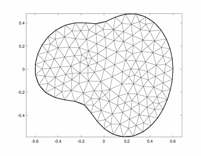
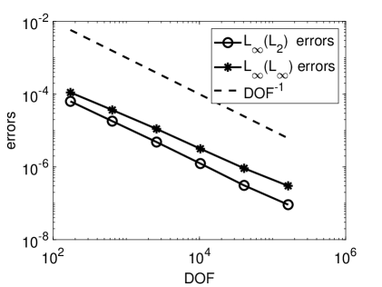
Figure 2. Fractional-order parabolic test problem: Delaunay triangulation of $\Omega$ with DOF=172 (left), maximum $L_{2}(\Omega)$ and $L_{\infty}(\Omega)$ errors for $\alpha=0.5$, $r=(3-\alpha)/\alpha$ and $M=2048$.

6.1. Parabolic case

Our fractional-order parabolic test problem is (1.3) with ${\mathcal{L}}=-(\partial_{x_{1}}^{2}+\partial_{x_{2}}^{2})+\color[rgb]{0,0,0.7}(1+|x|^{2})$, posed in the domain $\Omega\times[0,1]$ (see Fig. 2, left) with $\partial\Omega$ parameterized by $x_{1}(l):=\frac{2}{3}R\cos\theta$ and $x_{2}(l):=R\sin\theta$, where $R(l):=0.4+0.5\cos^{2}\!l$ and $\theta(l):=l+e^{(l-5)/2}\sin(l/2)\sin l$ for $l\in[0,2\pi]$; see [8, §7]. We choose $f$, as well as the initial and non-homogeneous boundary conditions, so that the unique exact solution $u=t^{\alpha}\cos(xy)$. This problem is discretized by (5.4) (with an obvious modification for the case of non-homogeneous boundary conditions) using lumped-mass linear finite elements on quasiuniform Delaunay triangulations of $\Omega$ (with DOF denoting the number of degrees of freedom in space).

The errors in the maximum $L_{2}(\Omega)$ norm are shown in Fig. 2 (right) and Table 1 for, respectively, a large fixed $M$ and DOF. In the latter case, we also give computational rates of convergence. The errors were computed using the piecewise-linear interpolant $u^{I}\in S_{h}$ in $\Omega$ of the exact solution as $\max_{m=1,\ldots,M}\|u_{h}-u^{I}\|_{L_{2}(\Omega)}$. The graded temporal mesh $\{t_{j}=T(j/M)^{r}\}_{j=0}^{M}$ was used with the optimal $r=(3-\alpha)/\alpha$; see Remark 4.3. In view of the latter remark, by Corollary 5.6, the errors are expected to be $\lesssim M^{-(3-\alpha)}+h^{2}$, where $h^{2}\simeq\mbox{DOF}^{-1}$. Our numerical results clearly confirm the sharpness of this corollary for the considered case.

Fig. 2 (right) also shows the errors in the maximum $L_{\infty}(\Omega)$ norm. Although it is not clear how the error analysis of Section 5 can be generalized for this case, it is worth noting that our numerical results (in Fig. 2, as well as a version of Table 1 for this case) suggest that the errors in the maximum $L_{\infty}(\Omega)$ norm are $\lesssim M^{-(3-\alpha)}+h^{2}|\ln h|$.

Table 1. Fractional-order parabolic test problem: maximum $L_{2}(\Omega)$ errors (odd rows) and computational rates $q$ in $M^{-q}$ (even rows) for $r=(3-\alpha)/\alpha$ and spatial DOF=255435

		$M=32$	$M=64$	$M=128$	$M=256$	$M=512$	$M=1024$
$\alpha=0.3$		4.885e-2	8.787e-3	1.426e-3	2.239e-4	3.470e-5	5.353e-6
		2.475	2.623	2.672	2.690	2.697
$\alpha=0.5$		2.305e-3	4.802e-4	9.012e-5	1.631e-5	2.911e-6	5.164e-7
		2.263	2.414	2.466	2.486	2.495
$\alpha=0.7$		7.683e-4	2.030e-4	4.561e-5	9.772e-6	2.030e-6	4.163e-7
		1.920	2.154	2.223	2.267	2.286

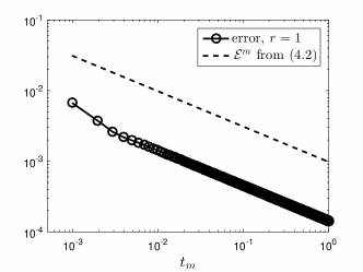
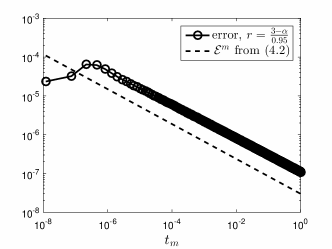
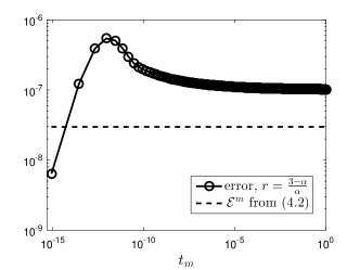
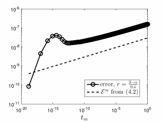
Figure 3. Initial-value test problem: pointwise errors for $\alpha=0.5$ and $M=1024$, cases $r=1$, $r=(3-\alpha)/0.95$, $r=(3-\alpha)/\alpha$ and $r=(3-\alpha)/0.4$.

Table 2. Initial-value test problem: errors at $t=1$ (odd rows) and computational rates $q$ in $M^{-q}$ (even rows) for $r=1$, $r=(3-\alpha)/.95$ and $r=(3-\alpha)/\alpha$

		$\;\;\;M=2^{5}$	$M=2^{7}$	$M=2^{9}$	$M=2^{11}$	$M=2^{13}$	$M=2^{15}$
$r=1$	$\alpha=0.3$	3.324e-3	8.297e-4	2.073e-4	5.182e-5	1.296e-5	3.239e-6
		1.001	1.000	1.000	1.000	1.000
	$\alpha=0.5$	4.557e-3	1.141e-3	2.852e-4	7.132e-5	1.783e-5	4.457e-6
		0.999	1.000	1.000	1.000	1.000
	$\alpha=0.7$	4.501e-3	1.127e-3	2.818e-4	7.047e-5	1.762e-5	4.405e-6
		0.999	1.000	1.000	1.000	1.000
$r=\frac{3-\alpha}{.95}$	$\alpha=0.3$	1.570e-4	3.435e-6	7.601e-8	1.701e-9	3.843e-11	8.771e-13
		2.757	2.749	2.741	2.734	2.727
	$\alpha=0.5$	5.440e-4	1.828e-5	6.038e-7	1.972e-8	6.384e-10	2.053e-11
		2.447	2.460	2.468	2.474	2.480
	$\alpha=0.7$	9.278e-4	4.524e-5	2.101e-6	9.477e-8	4.191e-9	1.827e-10
		2.179	2.214	2.235	2.249	2.260
$r=\frac{3-\alpha}{\alpha}$	$\alpha=0.3$	8.360e-4	1.481e-5	2.950e-7	6.248e-9	1.373e-10	3.088e-12
		2.910	2.825	2.781	2.754	2.737
	$\alpha=0.5$	7.448e-4	1.973e-5	5.839e-7	1.788e-8	5.541e-10	1.726e-11
		2.619	2.539	2.515	2.506	2.503
	$\alpha=0.7$	9.391e-4	3.381e-5	1.320e-6	5.339e-8	2.188e-9	9.009e-11
		2.398	2.340	2.314	2.304	2.301

Table 3. Initial-value test problem: maximum nodal errors (odd rows) and computational rates $q$ in $M^{-q}$ (even rows) for $r=1$, $r=3-\alpha$ and $r=(3-\alpha)/\alpha$

		$\;\;\;M=2^{5}$	$M=2^{7}$	$M=2^{9}$	$M=2^{11}$	$M=2^{13}$	$M=2^{15}$
$r=1$	$\alpha=0.3$	6.524e-2	4.304e-2	2.840e-2	1.873e-2	1.236e-2	8.155e-3
		0.300	0.300	0.300	0.300	0.300
	$\alpha=0.5$	3.794e-2	1.897e-2	9.484e-3	4.742e-3	2.371e-3	1.186e-3
		0.500	0.500	0.500	0.500	0.500
	$\alpha=0.7$	1.631e-2	6.180e-3	2.342e-3	8.874e-4	3.363e-4	1.274e-4
		0.700	0.700	0.700	0.700	0.700
$r=3-\alpha\;\;$	$\alpha=0.3$	2.131e-2	6.934e-3	2.256e-3	7.339e-4	2.388e-4	7.768e-5
		0.810	0.810	0.810	0.810	0.810
	$\alpha=0.5$	6.185e-3	1.093e-3	1.933e-4	3.417e-5	6.040e-6	1.068e-6
		1.250	1.250	1.250	1.250	1.250
	$\alpha=0.7$	1.867e-3	2.004e-4	2.151e-5	2.308e-6	2.477e-7	2.659e-8
		1.610	1.610	1.610	1.610	1.610
$r=\frac{3-\alpha}{\alpha}$	$\alpha=0.3$	6.510e-2	1.542e-3	3.652e-5	8.648e-7	2.048e-8	4.851e-10
		2.700	2.700	2.700	2.700	2.700
	$\alpha=0.5$	3.142e-3	9.820e-5	3.069e-6	9.590e-8	2.997e-9	9.365e-11
		2.500	2.500	2.500	2.500	2.500
	$\alpha=0.7$	1.273e-3	5.247e-5	2.164e-6	8.922e-8	3.679e-9	1.517e-10
		2.300	2.300	2.300	2.300	2.300

6.2. Pointwise sharpness of error estimate for the initial-value problem

Here, to demonstrate the sharpness of the error estimate (4.2) given by Theorem 4.1, we consider the simplest initial-value fractional-derivative test problem (4.1) with the simplest typical exact solution $u(t):=t^{\alpha}$. Table 2 shows the errors and the corresponding convergence rates at $t=1$, which agree with (4.2), in view of Remark 4.2. In particular, the latter implies that the errors are $\lesssim M^{-\min\{r,3-\alpha\}}$ for $r\neq 3-\alpha$. The maximum errors and corresponding convergence rates given in Table 3 clearly confirm the conclusions of Remark 4.3, which predicts from the pointwise bound (4.2) that the global errors are $\lesssim M^{-\min\{\alpha r,3-\alpha\}}$. Furthermore, in Fig. 3, the pointwise errors for various $r$ are compared with the pointwise theoretical error bound (4.2), and again, with the exception of a few initial mesh nodes, we observe remarkably good agreement. Note that Fig. 3 only addresses the case $\alpha=0.5$, but for other values of $\alpha$ we observed similar consistency of (4.2) with the actual pointwise errors.

References

- [1] S. C. Brenner and L. R. Scott, The mathematical theory of finite element methods, Springer-Verlag, New York, third ed., 2008.
- [2] H. Chen and M. Stynes, Error analysis of a second-order method on fitted meshes for a time-fractional diffusion problem, J. Sci. Comput. 79 (2019), 624–647.
- [3] K. Diethelm, The analysis of fractional differential equations, Lecture Notes in Mathematics, Springer-Verlag, Berlin, 2010.
- [4] G. Gao, Z. Sun and H. Zhang, A new fractional numerical differentiation formula to approximate the Caputo fractional derivative and its applications, J. Comput. Phys. 259 (2014), 33–50.
- [5] J. L. Gracia, E. O’Riordan and M. Stynes, Convergence in positive time for a finite difference method applied to a fractional convection-diffusion problem, Comput. Methods Appl. Math. 18 (2018), 33–42
- [6] B. Jin, R. Lazarov and Z. Zhou, Two fully discrete schemes for fractional diffusion and diffusion-wave equations with nonsmooth data, SIAM J. Sci. Comput. 38 (2016), A146–A170.
- [7] B. Jin, R. Lazarov and Z. Zhou, Numerical methods for time-fractional evolution equations with nonsmooth data: a concise overview, Comput. Methods Appl. Mech. Engrg. 346 (2019), 332–358.
- [8] N. Kopteva, Error analysis of the L1 method on graded and uniform meshes for a fractional-derivative problem in two and three dimensions, Math. Comp. (2019), published electronically 23-Jan-2019; doi: 10.1090/mcom/3410.
- [9] N. Kopteva and X. Meng, Error analysis for a fractional-derivative parabolic problem on quasi-graded meshes using barrier functions, SIAM J. Numer. Anal., 58 (2020), 1217–1238.
- [10] C. Lv and C. Xu, Error analysis of a high order method for time-fractional diffusion equations, SIAM J. Sci. Comput. 38 (2016), A2699–A2724.
- [11] M. Stynes, Too much regularity may force too much uniqueness, Fract. Calc. Appl. Anal. 19 (2016), 1554–1562.
- [12] M. Stynes, E. O’Riordan and J. L. Gracia, Error analysis of a finite difference method on graded meshes for a time-fractional diffusion equation, SIAM J. Numer. Anal. 55 (2017), 1057–1079.
- [13] Y. Xing and Y. Yan, A higher order numerical method for time fractional partial differential equations with nonsmooth data, J. Comput. Phys. 357 (2018), 305–323.