On the Computation and Communication Complexity of Parallel SGD with Dynamic Batch Sizes for Stochastic Non-Convex Optimization

Abstract

For SGD based distributed stochastic optimization, computation complexity, measured by the convergence rate in terms of the number of stochastic gradient calls, and communication complexity, measured by the number of inter-node communication rounds, are two most important performance metrics. The classical data-parallel implementation of SGD over $N$ workers can achieve linear speedup of its convergence rate but incurs an inter-node communication round at each batch. We study the benefit of using dynamically increasing batch sizes in parallel SGD for stochastic non-convex optimization by charactering the attained convergence rate and the required number of communication rounds. We show that for stochastic non-convex optimization under the P-L condition, the classical data-parallel SGD with exponentially increasing batch sizes can achieve the fastest known $O(1/(NT))$ convergence with linear speedup using only $\log(T)$ communication rounds. For general stochastic non-convex optimization, we propose a Catalyst-like algorithm to achieve the fastest known $O(1/\sqrt{NT})$ convergence with only $O(\sqrt{NT}\log(\frac{T}{N}))$ communication rounds.

1 Introduction

Consider solving the following stochastic optimization

$$\min_{{\mathbf{x}}\in{\mathbb{R}}^{m}}\quad f({\mathbf{x}})\overset{\Delta}{=}{\mathbb{E}}_{\zeta\sim{\mathcal{D}}}[F({\mathbf{x}};\zeta)]$$ (1)

with a fixed yet unknown distribution ${\mathcal{D}}$ only by accessing i.i.d. stochastic gradients $\nabla F(\cdot;\zeta)$. Most machine learning applications can be cast into the above stochastic optimization where ${\mathbf{x}}$ refers to the machine learning model, random variables $\zeta\sim{\mathcal{D}}$ refer to instance-label pairs and $F({\mathbf{x}};\zeta)$ refers to the corresponding loss function. For example, consider a simple least squares linear regression problem: let $\zeta_{i}=({\mathbf{a}}_{i},b_{i})\in{\mathcal{D}}$ be training data collected offline or online, where each ${\mathbf{a}}_{i}$ is a feature vector and $b_{i}$ is its label, then $F({\mathbf{x}};\zeta_{i})=\frac{1}{2}({\mathbf{a}}_{i}^{\mkern-1.5mu\mathsf{T}}{\mathbf{x}}-b_{i})^{2}$. Throughout this paper, we have the following assumption:

Assumption 1.

1. Smoothness: The objective function $f({\mathbf{x}})$ in problem (1) is smooth with modulus $L$.

2. Unbiased gradients with bounded variances: Assume there exits a stochastic first-order oracle (SFO) to provide independent unbiased stochastic gradients $\nabla F({\mathbf{x}};\zeta)$ satisfying

   $${\mathbb{E}}_{\zeta\sim{\mathcal{D}}}[\nabla F({\mathbf{x}};\zeta)]=\nabla f({\mathbf{x}}),\forall{\mathbf{x}}.$$

   The unbiased stochastic gradients have a bounded variance, i.e., there exits a constant $\sigma>0$ such that

   $${\mathbb{E}}_{\zeta\sim{\mathcal{D}}}\|{\nabla F({\mathbf{x}};\zeta)-\nabla f(\mathbf{x})}\|^{2}\leq\sigma^{2}$$ (2)

When solving stochastic optimization (1) only with sampled stochastic gradients, the computation complexity, which is also known as the convergence rate, is measured by the decay law of the solution error with respect to the number of access of the stochastic first-order oracle (SFO) that provides sampled stochastic gradients (Nemirovsky & Yudin, 1983; Ghadimi et al., 2016). For strongly convex stochastic minimization, SGD type algorithms (Nemirovski et al., 2009; Hazan & Kale, 2014; Rakhlin et al., 2012) can achieve the optimal $O(1/T)$ convergence rate. That is, the error is ensured to be at most $O(1/T)$ after $T$ access of stochastic gradients. For non-convex stochastic minimization, which is the case of training deep neural networks, SGD type algorithms can achieve an $O(1/\sqrt{T})$ convergence rate. Classical SGD type algorithms can be accelerated by utilizing multiple workers/nodes to follow a parallel SGD (PSGD) procedure where each worker computes local stochastic gradients in parallel, aggregates all local gradients, and updates its own local solution using the average of all gradients. Such a data-parallel training strategy with $N$ workers has $O(1/(NT))$ convergence for strongly convex minimization and $O(1/\sqrt{NT})$ convergence for smooth non-convex stochastic minimization, both of which is $N$ times faster than SGD with a single worker (Dekel et al., 2012; Ghadimi & Lan, 2013; Lian et al., 2015). This is known as the linear speedup (with respect to the number of nodes) property of PSGD.

However, such linear speedup is often not attainable in practice because PSGD involves additional coordination and communication cost as most other distributed/parallel algorithms do. In particular, PSGD requires aggregating local batch gradients among all workers after evaluations of local batch SGD. The corresponding communication cost for gradient aggregations is quite heavy and often becomes the performance bottleneck.

Since the number of inter-node communication rounds in PSGD over multiple nodes is equal to the number of batches, it is desirable to use larger batch sizes to avoid communication overhead as long as the large batch size does not damage the overall computation complexity (in terms of number of access of SFO). For training deep neural networks, practitioners have observed that SGD using dynamically increasing batch sizes can converges to similar test accuracy with the same number of epochs but significantly fewer number of batches when compared with SGD with small batch sizes (Devarakonda et al., 2017; Smith et al., 2018). The idea of using large or increasing batch sizes can be partially backed by some recent theoretical works (Bottou et al., 2018; De et al., 2017). It is shown in (De et al., 2017) that if the batch size is sufficiently large such that the randomness, i.e., variances, is dominated by gradient magnitude, then SGD essentially degrades to deterministic gradient descent. However, in the worst case, e.g., stochastic optimization (1) or large-scale optimization with limited budgets of SFO access, SGD with large batch sizes considered in (De et al., 2017) can have worse convergence performance than SGD with fixed small batch sizes (Bottou & Bousquet, 2008; Bottou et al., 2018). For strongly convex stochastic minimization, it is proven in (Friedlander & Schmidt, 2012; Bottou et al., 2018) that SGD with exponentially increasing batch sizes can achieve the same $O(1/T)$ convergence as SGD with fixed small batch sizes, where $T$ is the number of access of SFO. The results in (Friedlander & Schmidt, 2012; Bottou et al., 2018) are encouraging since it means using exponentially increasing batch sizes can preserve the low $O(1/T)$ computation complexity with $\log(T)$ communication complexity that is significantly lower than $O(T)$ required by SGD with fixed batch sizes for distributed strongly convex stochastic minimization. However, the computation and communication complexity remains under-explored for distributed stochastic non-convex optimization, which is the case of training deep neural networks. While work (Smith & Le, 2018; Smith et al., 2018) justify SGD with increasing batch sizes by relating it with the integration of a stochastic differential equation for which decreasing learning rates can roughly compensate the effect of increasing batch sizes, rigorous theoretical characterization on its computation and communication complexity (as in (Nemirovski et al., 2009; Bottou et al., 2018)) is missing for stochastic non-convex optimization. In general, it remains unclear “If using dynamic batch sizes in parallel SGD can yield the same fast $O(1/\sqrt{NT})$ convergence rate (with linear speedup with respect to the number of nodes) as the classical PSGD for non-convex optimization?” and “What is the corresponding communication complexity of using dynamic batch sizes to solve distributed non-convex optimization?”

Our Contributions: This paper aims to characterize both computation and communication complexity when using the idea of dynamically increasing batch sizes in SGD to solve stochastic non-convex optimization with $N$ parallel workers. We first consider non-convex optimization satisfying the Polyak-Lojasiewicz (P-L) condition, which can be viewed as a generalization of strong convexity for non-convex optimization. We show that by simply exponentially increasing the batch sizes at each worker (formally described in Algorithm 1) in the classical data-parallel SGD, we can solve non-convex optimization with the fast $O(1/(NT))$ convergence using only $O(\log(T))$ communication rounds. For general stochastic non-convex optimization (without P-L condition), we propose a Catalyst-like (Lin et al., 2015; Paquette et al., 2018) approach (formally described in Algorithm 2) that wraps Algorithm 1 with an outer loop that iteratively introduces auxiliary problems. We show that Algorithm 2 can solves general stochastic non-convex optimization with $O(1/\sqrt{NT})$ computation complexity and $O(\sqrt{TN}\log(\frac{T}{N}))$ communication complexity. In both cases, using dynamic batch sizes can achieve the linear speedup of convergence with communication complexity less than that of existing communication efficient parallel SGD methods with fixed batch sizes (Stich, 2018; Yu et al., 2018).

2 Non-Convex Minimization Under the P-L Condition

This section considers problem (1) satisfying the Polyak-Lojasiewicz (P-L) condition defined in Assumption 2.

Assumption 2.

The objective function $f({\mathbf{x}})$ in problem (1) satisfies the Polyak-Lojasiewicz (P-L) condition with modulus $\mu>0$. That is,

$$\frac{1}{2}\|{\nabla f({\mathbf{x}})}\|^{2}\geq\mu(f({\mathbf{x}})-f^{\ast}),\forall{\mathbf{x}}$$ (3)

where $f^{\ast}$ is the global minimum in problem (1).

The P-L condition is originally introduced by Polyak in (Polyak, 1963) and holds for many machine learning models. Neither the convexity of $f({\mathbf{x}})$ nor the uniqueness of its global minimizer is required in the P-L condition. In particular, the P-L condition is weaker than many other popular conditions, e.g., strong convexity and the error bound condition, used in optimization literature (Karimi et al., 2016). See e.g. Fact 1.

Fact 1 (Appendix A in (Karimi et al., 2016)).

If smooth function $\phi:{\mathbb{R}}^{m}\mapsto{\mathbb{R}}$ is strongly convex with modulus $\mu>0$, then it satisifes the P-L condition with the same modulus $\mu$.

One important example is: $f({\mathbf{x}})=g({\mathbf{Ax}})$ with strongly convex $g(\cdot)$ and possibly rank deficient matrix ${\mathbf{A}}$, e.g. $f({\mathbf{x}})=\|{{\mathbf{Ax}}-{\mathbf{b}}}\|^{2}$ used in least squares regressions. While $f({\mathbf{x}})=g({\mathbf{Ax}})$ is not strongly convex when ${\mathbf{A}}$ is rank deficient, it turns out that such $f({\mathbf{x}})$ always satisfies the P-L condition (Karimi et al., 2016).

Consider the Communication Reduced Parallel Stochastic Gradient Descent (CR-PSGD) algorithm described in Algorithm 1. The inputs of CR-PSGD are: (1) $N$, the number of parallel workers; (2) $T$, the total number of gradient evaluations at each worker; (3) ${\mathbf{x}}_{1}$, the common initial point at each worker; (3) $\gamma>0$, the learning rate; (4) $B_{1}$, the initial SGD batch size at each worker; (5) $\rho>1$, the batch size scaling factor. Compared with the classical PSGD, our CR-PSGD has the minor change that each worker exponentially increases its own SGD batch size with a factor $\rho$. Since $B_{t}$ increasingly exponentially, it is easy to see that the “while” loop in Algorithm 1 terminates after at most $O(\log T)$ steps. Meanwhile, we note that inter-worker communication is used only to aggregate individual batch SGD averages and happens only once in each “while” loop iteration. As a consequence, CR-PSGD only involves $O(\log T)$ rounds of communication. The remaining part of this section further proves that CR-PSGD has $O(1/(NT))$ convergence.

Similar ideas of exponentially increasing batch size appear in other works, e.g., (Hazan & Kale, 2014; Zhang et al., 2013), for different purposes and with different algorithm dynamics. In this paper, we explore this idea in the context of parallel stochastic optimization. It is impressive that such a simple idea enables us to obtain a parallel algorithm to achieve the fast $O(1/(NT))$ convergence with only $O(\log T)$ rounds of communication for stochastic optimization under the P-L condition. When considering stochastic strongly convex minimization that is a subclass of stochastic optimization under the P-L condition, the $O(\log T)$ communication complexity attained by our CR-PSGD is significantly less than the $O(\sqrt{NT})$ communication complexity attained by the local SGD method in (Stich, 2018).

Algorithm 1 $\text{CR-PSGD}(f,N,T,{\mathbf{x}}_{1},B_{1},\rho,\gamma)$

1:  Input: $N$, $T$, ${\mathbf{x}}_{1}\in\mathbb{R}^{m}$, $\gamma$ , $B_{1}$ and $\rho>1$.

2:  Initialize $t=1$

3:  while $\sum_{\tau=1}^{t}B_{\tau}\leq T$ do

4:     Each worker $i$ observes $B_{t}$ unbiased i.i.d. stochastic gradients at point ${\mathbf{x}}_{t}$ given by ${\mathbf{g}}_{i,j}\overset{\Delta}{=}\nabla F({\mathbf{x}}_{t};\zeta_{i,j}),j\in\{1,\ldots,B_{t}\},\zeta_{i,j}\sim{\mathcal{D}}$ and calculates its batch SGD average $\bar{{\mathbf{g}}}_{t,i}=\frac{1}{B_{t}}\sum_{j=1}^{B_{t}}{\mathbf{g}}_{i,j}$.

5:     Aggregate all $\bar{{\mathbf{g}}}_{t,i}$ from $N$ workers and compute their average $\bar{{\mathbf{g}}}_{t}=\frac{1}{N}\sum_{i=1}^{N}\bar{{\mathbf{g}}}_{t,i}$.

6:     Update ${\mathbf{x}}_{t+1}$ over all $N$ workers in parallel via: ${\mathbf{x}}_{t+1}={\mathbf{x}}_{t}-\gamma\bar{{\mathbf{g}}}_{t}$.

7:     Set $B_{t+1}=\lfloor\rho^{t}B_{1}\rfloor$ where $\lfloor z\rfloor$ represents the largest integer no less than $z$.

8:     Update $t\leftarrow t+1$.

9:  end while

10:  Return: $\mathbf{x}_{t}$

The next simple lemma relates per-iteration error with the batch sizes and is a key property to establish the convergence rate of Algorithm 1.

Lemma 1.

Consider problem (1) under Assumptions 1-2. If we choose $\gamma<\frac{1}{L}$ in Algorithm 1, then for all $t\in\{1,2,\ldots,\}$, we have

$${\mathbb{E}}[f({\mathbf{x}}_{t+1})-f^{\ast})]\leq(1-\nu){\mathbb{E}}[f({\mathbf{x}}_{t})-f^{\ast}]+\frac{\gamma(2-L\gamma)}{2NB_{t}}\sigma^{2}$$ (4)

where $f^{\ast}$ is the global minimum in problem (1) and $\nu\overset{\Delta}{=}\frac{1}{2}\gamma\mu(1-L\gamma)$ satisfies $0<\nu<1$.

Proof.

Fix $t\geq 1$. By the smoothness of $f({\mathbf{x}})$ in Assumption 1, we have

$$f({\mathbf{x}}_{t+1})$$

$$\leq f({\mathbf{x}}_{t})+\langle\nabla f({\mathbf{x}}_{t}),{\mathbf{x}}_{t+1}-{\mathbf{x}}_{t}\rangle+\frac{L}{2}\|{{\mathbf{x}}_{t+1}-{\mathbf{x}}_{t}}\|^{2}$$

$$\overset{(a)}{=} f({\mathbf{x}}_{t})-\gamma\langle\nabla f({\mathbf{x}}_{t}),\bar{{\mathbf{g}}}_{t}\rangle+\frac{L}{2}\gamma^{2}\|{\bar{{\mathbf{g}}}_{t}}\|^{2}$$

$$= f({\mathbf{x}}_{t})+\gamma\langle\bar{{\mathbf{g}}}_{t}-\nabla f({\mathbf{x}}_{t}),\bar{{\mathbf{g}}}_{t}\rangle-\gamma\|{\bar{{\mathbf{g}}}_{t}}\|^{2}+\frac{L}{2}\gamma^{2}\|{\bar{{\mathbf{g}}}_{t}}\|^{2}$$

$$\overset{(b)}{\leq} f({\mathbf{x}}_{t})+\frac{\gamma}{2}\|{\bar{{\mathbf{g}}}_{t}-\nabla f({\mathbf{x}}_{t})}\|^{2}+\frac{\gamma}{2}(L\gamma-1)\|{\bar{{\mathbf{g}}}_{t}}\|^{2}$$

$$\overset{(c)}{\leq} f({\mathbf{x}}_{t})+\frac{\gamma}{4}(L\gamma-1)\|{\nabla f({\mathbf{x}}_{t})}\|^{2}+\frac{\gamma}{2}(2-L\gamma)\|{\bar{{\mathbf{g}}}_{t}-\nabla f({\mathbf{x}}_{t})}\|^{2}$$

$$\overset{(d)}{\leq} f({\mathbf{x}}_{t})+\frac{1}{2}\gamma\mu(L\gamma-1)(f({\mathbf{x}}_{t})-f^{\ast})$$

$$\quad+\frac{\gamma}{2}(2-L\gamma)\|{\bar{{\mathbf{g}}}_{t}-\nabla f({\mathbf{x}}_{t})}\|^{2}$$ (5)

where (a) follows by substituting ${\mathbf{x}}_{t+1}={\mathbf{x}}_{t}-\gamma\bar{{\mathbf{g}}}_{t}$; (b) follows by applying elementary inequality $\langle{\mathbf{u}},{\mathbf{v}}\rangle\leq\frac{1}{2}\|{{\mathbf{u}}}\|^{2}+\frac{1}{2}\|{{\mathbf{v}}}\|^{2}$ with ${\mathbf{u}}=\bar{{\mathbf{g}}}_{t}-\nabla f({\mathbf{x}}_{t})$ and ${\mathbf{v}}=\bar{{\mathbf{g}}}_{t}$; (c) follows by noting that $L\gamma-1<0$ under our selection of $\gamma$ and applying elementary inequality $\|{{\mathbf{u}}+{\mathbf{v}}}\|^{2}\geq\frac{1}{2}\|{{\mathbf{u}}}\|^{2}-\|{{\mathbf{v}}}\|^{2}$ with ${\mathbf{u}}=\nabla f({\mathbf{x}}_{t})$ and ${\mathbf{v}}=\bar{{\mathbf{g}}}_{t}-\nabla f({\mathbf{x}}_{t})$; and (d) follows by noting that $\gamma(L\gamma-1)<0$ under our selection of $\gamma$ and $\|{\nabla f({\mathbf{x}}_{t})}\|^{2}\geq 2\mu(f({\mathbf{x}}_{t})-f^{\ast})$ by Assumption 2.

Defining $\nu\overset{\Delta}{=}\frac{1}{2}\gamma\mu(1-L\gamma)$, subtracting $f^{\ast}$ from both sides of (5), and rearranging terms yields

$$f({\mathbf{x}}_{t+1})-f^{\ast}$$

$$\leq (1-\nu)(f({\mathbf{x}}_{t})-f^{\ast})+\frac{\gamma}{2}(2-L\gamma)\|{\bar{{\mathbf{g}}}_{t}-\nabla f({\mathbf{x}}_{t})}\|^{2}$$ (6)

Taking expectations on both sides and noting that ${\mathbb{E}}[\|{\bar{{\mathbf{g}}}_{t}-\nabla f({\mathbf{x}}_{t})}\|^{2}]\leq\frac{1}{NB_{t}}\sigma^{2}$, which further follows from Assumption 1 and the fact that each $\bar{{\mathbf{g}}}_{t}$ is the average of $NB_{t}$ i.i.d. stochastic gradients evaluated at the same point, yields

$${\mathbb{E}}[f({\mathbf{x}}_{t+1})-f^{\ast}]\leq(1-\nu){\mathbb{E}}[f({\mathbf{x}}_{t})-f^{\ast}]+\frac{\gamma(2-L\gamma)}{2NB_{t}}\sigma^{2}$$

It remains to verify why $0<\nu<1$. Since $\gamma<\frac{1}{L}$, it is easy to see $\nu>0$. Next, we show $\frac{1}{2}\gamma\mu(1-L\gamma)<1$. By the smoothness of $f({\mathbf{x}})$ (and Fact 3 in Supplement 6.1), we have

$$\frac{1}{2}\|{\nabla f({\mathbf{x}})}\|^{2}\leq L(f({\mathbf{x}})-f^{\ast}),\forall{\mathbf{x}}$$ (7)

By Assumption 2, we have

$$\frac{1}{2}\|{\nabla f({\mathbf{x}})}\|^{2}\geq\mu(f({\mathbf{x}})-f^{\ast}),\forall{\mathbf{x}}$$ (8)

Inequalities (7) and (8) together imply that $\mu\leq L$, which further implies that $\frac{1}{2}\gamma\mu(1-L\gamma)\leq\frac{1}{2}\gamma L(1-L\gamma)<1$. ∎

Remark 1.

Note that by adapting steps (b) and (c) of (5) in the proof of Lemma 1, i.e., using inequalities with slightly different coefficients for the squared norm terms, we can obtain (4) with different $\nu$ values. Larger $\nu$ variants (with possibly more stringent conditions on the selection rule of $\gamma$) may lead to faster convergence (but with the same order) of Algorithm 1. This paper does not explore further in this direction since the current simple analysis is already sufficient to provide the desired order of convergence/communication. The suggested finer development on $\nu$ can improve the constant factor in the rates but does not improve their order. Nevertheless, it is worthwhile to point out that the finer development on $\nu$ can be helpful to guide practitioners to tune Algorithm 1 according to their specific minimization problems.

The $O(\frac{1}{NT})$ convergence with $O(\log T)$ communication rounds is summarized in Theorem 1.

Theorem 1.

Consider problem (1) under Assumptions 1-2. Let $T>0$ be a given constant. If we choose $B_{1}\geq 2$, $\gamma<\frac{1}{L}$ and $1<\rho<\frac{1}{1-\nu}$, where $\nu\overset{\Delta}{=}\frac{1}{2}\gamma\mu(1-L\gamma)$, in Algorithm 1, then the final output ${\mathbf{x}}_{t}$ returned by Algorithm 1 satisfies

$${\mathbb{E}}[f({\mathbf{x}}_{t})-f^{\ast}]\leq \frac{c_{1}(f({\mathbf{x}}_{1})-f^{\ast})}{T^{1+\delta}}+\frac{c_{2}}{NT}$$

$$= O(\frac{1}{T^{1+\delta}})+O(\frac{1}{NT})$$ (9)

where $\delta\overset{\Delta}{=}\log_{\rho}(\frac{1}{1-\nu})-1>0$, $c_{1}\overset{\Delta}{=}\frac{1}{1-\nu}\big{(}\frac{B_{1}}{\rho-1}\big{)}^{1+\delta}$, $c_{2}\overset{\Delta}{=}\frac{\rho^{2}\gamma(2-L\gamma))\sigma^{2}}{(1-(1-\nu)\rho)(\rho-1)}$, and $f^{\ast}$ is the minimum value of problem (1).

Proof.

See Supplement 6.2. ∎

Remark 2.

Since $\delta>0$, $O(\frac{1}{T^{1+\delta}})$ decays faster than $O(\frac{1}{NT})$ when $T$ is sufficiently large. In fact, we can even explicitly choose suitable $\rho$ to make $\delta$ sufficiently large, e.g., we can choose $1<\rho<\sqrt{\frac{1}{1-\nu}}$ to ensure $\delta>1$ such that $O(\frac{1}{T^{1+\delta}})<O(\frac{1}{T^{2}})$. In this case, as long as $T\geq N$, which is almost always true in practice, the error term on the right side of (29) has order $O(\frac{1}{NT})$.

Recall that if $f({\mathbf{x}})$ is strongly convex with modulus $\mu$, then it satisfies Assumption 2 with the same $\mu$ by Fact 1. Furthermore, if $f({\mathbf{x}})$ is strongly convex with modulus $\mu>0$, we know problem (1) has a unique minimizer ${\mathbf{x}}^{\ast}$ and $\|{{\mathbf{x}}-{\mathbf{x}}^{\ast}}\|^{2}\leq\frac{2}{\mu}(f({\mathbf{x}})-f({\mathbf{x}}^{\ast}))$ for any ${\mathbf{x}}$. (See e.g. Fact 4 in Supplement 6.1.) Thus, we have the following corollary for Theorem 1.

Corollary 1.

Consider problem (1) under Assumptions 1 where $f({\mathbf{x}})$ is strongly convex with modulus $\mu>0$. Under the same conditions in Theorem 1, the final output ${\mathbf{x}}_{t}$ returned by Algorithm 1 satisfies

$${\mathbb{E}}[\|{{\mathbf{x}}_{t}-{\mathbf{x}}^{\ast}}\|^{2}]\leq \frac{2c_{1}(f({\mathbf{x}}_{1})-f({\mathbf{x}}^{\ast}))}{\mu T^{1+\delta}}+\frac{2c_{2}}{\mu NT}$$

$$= O(\frac{1}{T^{1+\delta}})+O(\frac{1}{NT})$$ (10)

where $\delta,c_{1},c_{2}$ are positive constants defined in Theorem 1 and ${\mathbf{x}}^{\ast}$ is the unique minimizer of problem (1).

Remark 3.

Recall that $O(1/T)$ convergence is optimal for stochastic strongly convex optimization (Nemirovsky & Yudin, 1983; Rakhlin et al., 2012) over single node. Since the convergence of Algorithm 1 scales out perfectly with respect to the number of involved workers and strongly convex functions are a subclass of functions satisfying the P-L condition, we can conclude the $O(\frac{1}{NT})$ convergence attained by Algorithm 1 is optimal for parallel stochastic optimization under the P-L condition. It is also worth noting that we consider general stochastic optimization (1) such that acceleration techniques developed for finite sum optimization, e.g., variance reduction, are excluded from consideration.

3 General Non-Convex Minimization

Let $f({\mathbf{x}})$ be the (stochastic) objective function in problem (1). For any given fixed ${\mathbf{y}}$, define a new function with respect to ${\mathbf{x}}$ given by

$$h_{\theta}({\mathbf{x}};{\mathbf{y}})\overset{\Delta}{=}f({\mathbf{x}})+\frac{\theta}{2}\|{{\mathbf{x}}-{\mathbf{y}}}\|^{2}$$ (11)

It is easy to verify that if $f({\mathbf{x}})$ is smooth with modulus $L$ and $\theta>L$, then $h_{\theta}({\mathbf{x}};{\mathbf{y}})$ is both smooth with modulus $\theta+L$ and strongly convex with modulus $\theta-L>0$. Furthermore, if $\nabla F({\mathbf{x}};\zeta)$ are unbiased i.i.d. stochastic gradients of function $f(\cdot)$ with a variance bounded by $\sigma^{2}$, then $\nabla F({\mathbf{x}};\zeta)+\theta({\mathbf{x}}-{\mathbf{y}})$ are unbiased i.i.d. stochastic gradients of $h_{\theta}({\mathbf{x}};{\mathbf{y}})$ with the same variance.

Algorithm 2 $\text{CR-PSGD-Catalyst}(f,N,T,{\mathbf{y}}_{0},B_{1},\rho,\gamma)$

1:  Input: $N$, $T$, $\theta$, ${\mathbf{y}}_{0}\in\mathbb{R}^{m}$, $\gamma$ , $B_{1}$ and $\rho>1$.

2:  Initialize ${\mathbf{y}}^{(0)}={\mathbf{y}}_{0}$ and $k=1$.

3:  while $k\leq\lfloor\sqrt{NT}\rfloor$ do

4:     Define $h_{\theta}({\mathbf{x}};{\mathbf{y}}^{(k-1)})$ using (11). Update ${\mathbf{y}}^{(k)}$ via

$${\mathbf{y}}^{(k)}=\text{CR-PSGD}(h_{\theta}(\cdot;{\mathbf{y}}^{(k-1)}),N,\lfloor\sqrt{T/N}\rfloor,{\mathbf{y}}^{(k-1)},B_{1},\rho,\gamma)$$

5:     Update $k\leftarrow k+1$.

6:  end while

Now consider Algorithm 2 that wraps CR-PSGD with an outer-loop that updates $h_{\theta}({\mathbf{x}};{\mathbf{y}}^{(k-1)})$ and applies CR-PSGD to minimize it. Note that $h_{\theta}({\mathbf{x}};{\mathbf{y}}^{(k-1)})$ augments the objective function $f({\mathbf{x}})$ with an iteratively updated proximal term $\frac{\theta}{2}\|{{\mathbf{x}}-{\mathbf{y}}^{(k-1)}}\|^{2}$. The introduction of proximal terms $\frac{\theta}{2}\|{{\mathbf{x}}-{\mathbf{y}}^{(k-1)}}\|^{2}$ is inspired by earlier works (Güler, 1992; He & Yuan, 2012; Salzo & Villa, 2012; Lin et al., 2015; Yu & Neely, 2017; Davis & Grimmer, 2017; Paquette et al., 2018) on proximal point methods, which solve an minimization problem by solving a sequence of auxiliary problems involving a quadratic proximal term. By choosing $\theta>L$ in (11), we can ensure $h_{\theta}({\mathbf{x}};{\mathbf{y}}^{(k-1)})$ is both smooth and strongly convex. For strongly convex $h_{\theta}({\mathbf{x}};{\mathbf{y}}^{(k-1)})$, Theorem 1 and Corollary 1 show that $\text{CR-PSGD}(N,\lfloor\sqrt{T/N}\rfloor,{\mathbf{y}}^{(k-1)},B_{1},\rho,\gamma)$ can return an $O(\frac{1}{\sqrt{NT}})$ approximated minimizer with only $O(\log(\frac{T}{N}))$ communication rounds. The ultimate goal of the proximal point like outer-loop introduced in Algorithm 2 is to lift the ”communication reduction” property from CR-PSGD for non-convex minimization under the restrictive PL condition to solve general non-convex minimization with reduced communication. Our method shares a similar philosophy with the “catalyst acceleration” in (Lin et al., 2015) which also uses a “proximal-point” outer-loop to achieve improved convergence rates for convex minimization by lifting fast convergence from strong convex minimization. In this perspective, we call Algorithm 2 “CR-PSGD-Catalyst” by borrowing the word “catalyst” from (Lin et al., 2015). While both Algorithm 2 and “catalyst acceleration” use an proximal point outer-loop to lift desired algorithmic properties from specific problems to generic problems, they are different in the following two aspects:

• The “catalyst acceleration” in (Lin et al., 2015; Paquette et al., 2018) is developed to accelerate a wide range of first-order deterministic minimization, e.g., gradient based methods and their randomized variants such as SAG, SAGA, SDCA, SVRG, for both convex and non-convex cases. In particular, it requires the existence of a subprocedure with linear convergence for strongly convex minimization. It is remarked in (Lin et al., 2015) that whether “catalyst” can accelerate stochastic gradient based methods for stochastic minimization in the sense of (Nemirovski et al., 2009) remains unclear. In contrast, our CR-PSGD-Catalyst can solve general stochastic minimization, which does not necessarily have a finite sum form, with i.i.d. stochastic gradients. The used CR-PSGD subprocedure that is different from linear converging subprocedure used in (Lin et al., 2015; Paquette et al., 2018).

• The “proximal point” outer loop used in “catalyst acceleration” is solely to accelerate convergence (Lin et al., 2015; Paquette et al., 2018). In contrast, the “proximal point” outer loop used in our CR-PSGD-Catalyst provides convergence acceleration and communication reduction simultaneously. Our analysis is also significantly different from analyses for conventional “catalyst acceleration”.

Since each call of CR-PSGD in Algorithm 2 requires only $O(\log(\frac{T}{N}))$ inter-worker communication rounds and there are $\sqrt{NT}$ calls of CR-PSGD, it is easy to see CR-PSGD-Catalyst in total uses $O(\sqrt{NT}\log(\frac{T}{N}))$ communication rounds. The $O(\sqrt{NT}\log(\frac{T}{N}))$ communication complexity of CR-PSGD-Catalyst for general non-convex stochastic optimization is significantly less than the $O(T)$ communication complexity attained by PSGD (Dekel et al., 2012; Ghadimi & Lan, 2013; Lian et al., 2015) or the $O(N^{3/4}T^{3/4})$ communication complexity required by local SGD (Yu et al., 2018). The next theorem summarizes that our CR-PSGD-Catalyst can achieve the fastest known $O(1/\sqrt{NT})$ convergence that is previously attained by the PSGD or local SGD.

Theorem 2.

Consider problem (1) under Assumption 1. If we choose $\theta>L$, $B_{1}\geq 2$, $\gamma<\frac{1}{\theta+L}$ and $1<\rho<\frac{1}{1-\nu}$, where $\nu\overset{\Delta}{=}\frac{1}{2}\gamma(\theta-L)(1-(\theta+L)\gamma)$, in Algorithm 2 and if $T\geq\max\{N,N\big{(}\frac{4c_{1}(\theta+L)^{2}}{(\theta-L)^{2}}\big{)}^{\frac{2}{1+\delta}},N(c_{1})^{\frac{2}{1+\delta}}\}$, then we have

$$\frac{1}{\sqrt{NT}}\sum_{k=1}^{\sqrt{NT}}{\mathbb{E}}[\|{\nabla f({\mathbf{y}}^{(k)})}\|^{2}]=O(\frac{1}{\sqrt{NT}})$$

where $\{{\mathbf{y}}^{(k)},k\geq 1\}$ are a sequence of solutions returned from the CR-PSGD subprocedure.

Proof.

For simplicity, we assume $\sqrt{NT}$ and $\sqrt{T/N}$ are integers and hence $\lfloor\sqrt{NT}\rfloor=\sqrt{NT}$ and $\lfloor\sqrt{T/N}\rfloor=\sqrt{T/N}$. This can be be ensured when $T=N^{3}q^{2}$ where $q$ is any integer. In general, even if $\sqrt{TN}$ or $\sqrt{T/N}$ are non-integers, by using the fact that $\frac{1}{2}z\leq\lfloor z\rfloor\leq z$ for any $z\geq 2$, the same order of convergence can be easily extended to the case when $\sqrt{NT}$ or $\sqrt{T/N}$ are non-integers.

Fix $k\geq 1$ and consider stochastic minimization $\min_{{\mathbf{x}}\in{\mathbb{R}}^{m}}h_{\theta}({\mathbf{x}};{\mathbf{y}}^{(k-1)})$. Since $h_{\theta}({\mathbf{x}};{\mathbf{y}}^{(k-1)})$ is strongly convex with modulus $\theta-L>0$, we know $h_{\theta}({\mathbf{x}};{\mathbf{y}}^{(k-1)})$ also satisfies the P-L condition with modulus $\theta-L$ by Fact 1. At the same time, $h_{\theta}({\mathbf{x}};{\mathbf{y}}^{(k-1)})$ is smooth with modulus $\theta+L$. Note that our selections of $B_{1},\gamma$ and $\rho$ satisfy the condition in Theorem 1 for stochastic minimization under the P-L condition. Denote ${\mathbf{y}}^{(k)}_{\ast}\overset{\Delta}{=}\underset{{\mathbf{x}}\in{\mathbb{R}}^{m}}{\mbox{argmin }}\{h_{\theta}({\mathbf{x}};{\mathbf{y}}^{(k-1)})\}.$

Recall that ${\mathbf{y}}^{(k)}$ is the solution returned from CR-PSGD with $\sqrt{T/N}$ iterations. By Theorem 1, we have

$${\mathbb{E}}[h_{\theta}({\mathbf{y}}^{(k)};{\mathbf{y}}^{(k-1)})-h_{\theta}({\mathbf{y}}^{(k)}_{\ast};{\mathbf{y}}^{(k-1)})]$$

$$\leq \frac{c_{1}}{(\frac{T}{N})^{\frac{1+\delta}{2}}}{\mathbb{E}}[h_{\theta}({\mathbf{y}}^{(k-1)};{\mathbf{y}}^{(k-1)})-h_{\theta}({\mathbf{y}}^{(k)}_{\ast};{\mathbf{y}}^{(k-1)})]+\frac{c_{2}}{\sqrt{NT}}$$ (12)

where $\delta\overset{\Delta}{=}\log_{\rho}(\frac{1}{1-\nu})-1>0$, $c_{1}\overset{\Delta}{=}\frac{1}{1-\nu}\big{(}\frac{B_{1}}{\rho-1}\big{)}^{1+\delta}$, and $c_{2}\overset{\Delta}{=}\frac{\rho^{2}\gamma(2-(\theta+L)\gamma))\sigma^{2}}{(1-(1-\nu)\rho)(\rho-1)}$ are absolute constants independent of $T$.

Since $h_{\theta}(\cdot;{\mathbf{y}}^{(k-1)})$ is smooth with modulus $\theta+L$ and ${\mathbf{y}}^{(k)}_{\ast}$ minimizes it, by Fact 3 (in Supplement 6.1), we have

$$\frac{1}{2(\theta+L)}\|{\nabla h_{\theta}({\mathbf{y}}^{(k)};{\mathbf{y}}^{(k-1)})}\|^{2}$$

$$\leq h_{\theta}({\mathbf{y}}^{(k)};{\mathbf{y}}^{(k-1)})-h_{\theta}({\mathbf{y}}^{(k)}_{\ast};{\mathbf{y}}^{(k-1)})$$ (13)

One the other hand ,we also have

$$h_{\theta}({\mathbf{y}}^{(k-1)};{\mathbf{y}}^{(k-1)})-h_{\theta}({\mathbf{y}}^{(k)}_{\ast};{\mathbf{y}}^{(k-1)})$$

$$\overset{(a)}{\leq} \frac{\theta+L}{2}\|{{\mathbf{y}}^{(k-1)}-{\mathbf{y}}^{(k)}_{\ast}}\|^{2}$$

$$\overset{(b)}{\leq} (\theta+L)\|{{\mathbf{y}}^{(k)}-{\mathbf{y}}^{(k)}_{\ast}}\|^{2}+(\theta+L)\|{{\mathbf{y}}^{(k)}-{\mathbf{y}}^{(k-1)}}\|^{2}$$

$$\overset{(c)}{\leq} \frac{\theta+L}{(\theta-L)^{2}}\|{\nabla h_{\theta}({\mathbf{y}}^{(k)};{\mathbf{y}}^{(k-1)})}\|^{2}+(\theta+L)\|{{\mathbf{y}}^{(k)}-{\mathbf{y}}^{(k-1)}}\|^{2}$$ (14)

where (a) follows from Fact 2 (in Supplement 6.1) by recalling again that $h_{\theta}(\cdot;{\mathbf{y}}^{(k-1)})$ is smooth with modulus $\theta+L$ and ${\mathbf{y}}^{(k)}_{\ast}$ minimizes it; (b) follows because $\|{{\mathbf{y}}^{(k-1)}-{\mathbf{y}}^{(k)}_{\ast}}\|^{2}\leq 2\|{{\mathbf{y}}^{(k)}-{\mathbf{y}}^{(k)}_{\ast}}\|^{2}+2\|{{\mathbf{y}}^{(k)}-{\mathbf{y}}^{(k-1)}}\|^{2}$, which further follows by applying basic inequality $\|{{\mathbf{u}}-{\mathbf{v}}}\|^{2}\leq 2\|{{\mathbf{u}}}\|^{2}+2\|{{\mathbf{v}}}\|^{2}$ with ${\mathbf{u}}={\mathbf{y}}^{(k)}-{\mathbf{y}}^{(k)}_{\ast}$ and ${\mathbf{v}}={\mathbf{y}}^{(k)}-{\mathbf{y}}^{(k-1)}$; and (c) follows because $\|{{\mathbf{y}}^{(k)}-{\mathbf{y}}^{(k)}_{\ast}}\|^{2}\leq\frac{1}{(\theta-L)^{2}}\|{\nabla h_{\theta}({\mathbf{y}}^{(k)};{\mathbf{y}}^{(k-1)})}\|^{2}$, which further follows from by Fact 5 (in Supplement 6.1) by noting that $h_{\theta}(\cdot;{\mathbf{y}}^{(k-1)})$ is strongly convex with modulus $\theta-L$ and ${\mathbf{y}}^{(k)}_{\ast}$ minimizes it.

Substituting (13) and (14) into (12) and rearranging terms yields

$$\Big{(}\underbrace{\frac{1}{2(\theta+L)}-\frac{c_{1}(\theta+L)}{(\theta-L)^{2}}\frac{1}{(\frac{T}{N})^{\frac{1+\delta}{2}}}}_{\overset{\Delta}{=}\alpha}\Big{)}{\mathbb{E}}[\|{\nabla h_{\theta}({\mathbf{y}}^{(k)};{\mathbf{y}}^{(k-1)})}\|^{2}]$$

$$\leq \frac{c_{1}(\theta+L)}{(\frac{T}{N})^{1+\delta}}{\mathbb{E}}]\|{{\mathbf{y}}^{(k)}-{\mathbf{y}}^{(k-1)}}\|^{2}]+\frac{c_{2}}{\sqrt{NT}}$$ (15)

Note that $T\geq N\big{(}\frac{4c_{1}(\theta+L)^{2}}{(\theta-L)^{2}}\big{)}^{\frac{2}{1+\delta}}$ ensures the term marked by an underbrace in (15) satisfies $\alpha\geq\frac{1}{4(\theta+L)}$. Thus, (15) implies that

$$\frac{1}{4(\theta+L)}{\mathbb{E}}[\|{\nabla h_{\theta}({\mathbf{y}}^{(k)};{\mathbf{y}}^{(k-1)})}\|^{2}]$$

$$\leq \frac{c_{1}(\theta+L)}{(\frac{T}{N})^{1+\delta}}{\mathbb{E}}]\|{{\mathbf{y}}^{(k)}-{\mathbf{y}}^{(k-1)}}\|^{2}]+\frac{c_{2}}{\sqrt{NT}}$$ (16)

By the definition of $h_{\theta}(\cdot;{\mathbf{y}}^{(k-1)})$, we have $\nabla h_{\theta}({\mathbf{y}}^{(k)};{\mathbf{y}}^{(k-1)})=\nabla f({\mathbf{y}}^{(k)})+\theta({\mathbf{y}}^{(k)}-{\mathbf{y}}^{(k-1)})$. This implies that

$$\|{\nabla f({\mathbf{y}}^{(k)})}\|^{2}\leq 2\|{\nabla h_{\theta}({\mathbf{y}}^{(k)};{\mathbf{y}}^{(k-1)})}\|^{2}+2\theta^{2}\|{{\mathbf{y}}^{(k)}-{\mathbf{y}}^{(k-1)}}\|^{2}$$ (17)

Combining (16) and (17) yields

$${\mathbb{E}}[\|{\nabla f({\mathbf{y}}^{(k)})}\|^{2}]$$

$$\leq \Big{(}\frac{8c_{1}(\theta+L)^{2}}{(\frac{T}{N})^{1+\delta}}+2\theta^{2}\Big{)}{\mathbb{E}}[\|{{\mathbf{y}}^{(k)}-{\mathbf{y}}^{(k-1)}}\|^{2}]+\frac{8c_{2}(\theta+L)}{\sqrt{NT}}$$

$$\overset{(a)}{\leq} \Big{(}8c_{1}(\theta+L)^{2}+2\theta^{2}\Big{)}{\mathbb{E}}[\|{{\mathbf{y}}^{(k)}-{\mathbf{y}}^{(k-1)}}\|^{2}]+\frac{8c_{2}(\theta+L)}{\sqrt{NT}}$$ (18)

where (a) follows because $(\frac{T}{N})^{1+\delta}\geq 1$ as long as $T\geq N$.

Since $T\geq Nc_{1}^{\frac{2}{1+\delta}}$ ensures $\frac{c_{1}}{(\frac{T}{N})^{\frac{1+\delta}{2}}}\leq 1$, by (12), we have

$${\mathbb{E}}[h_{\theta}({\mathbf{y}}^{(k)};{\mathbf{y}}^{(k-1)})-h_{\theta}({\mathbf{y}}^{(k)}_{\ast};{\mathbf{y}}^{(k-1)})]$$

$$\leq {\mathbb{E}}[h_{\theta}({\mathbf{y}}^{(k-1)};{\mathbf{y}}^{(k-1)})-h_{\theta}({\mathbf{y}}^{(k)}_{\ast};{\mathbf{y}}^{(k-1)})]+\frac{c_{2}}{\sqrt{NT}}$$ (19)

Cancelling the common term on both sides and substituting the definition of $h_{\theta}(\cdot;{\mathbf{y}}^{(k-1)})$ into (19) yields

$${\mathbb{E}}[f({\mathbf{y}}^{(k)})+\frac{\theta}{2}\|{{\mathbf{y}}^{(k)}-{\mathbf{y}}^{(k-1)}}\|^{2}]$$

$$\leq {\mathbb{E}}[f({\mathbf{y}}^{(k-1)})]+\frac{c_{2}}{\sqrt{NT}}$$ (20)

Rewriting this inequality as ${\mathbb{E}}[\|{{\mathbf{y}}^{(k)}-{\mathbf{y}}^{(k-1)}}\|^{2}]\leq\frac{2}{\theta}{\mathbb{E}}[f({\mathbf{y}}^{(k-1)})-f({\mathbf{y}}^{(k)})]+\frac{2c_{2}}{\theta\sqrt{NT}}$ and substituting it into (18) yields

$${\mathbb{E}}[\|{\nabla f({\mathbf{y}}^{(k)})}\|^{2}]$$

$$\leq \frac{2}{\theta}\Big{(}8c_{1}(\theta+L)^{2}+2\theta^{2}\Big{)}{\mathbb{E}}[f({\mathbf{y}}^{(k-1)})-f({\mathbf{y}}^{(k)})]$$

$$+\Big{(}\frac{16c_{1}(\theta+L)^{2}}{\theta}+12\theta+8L\Big{)}\frac{c_{2}}{\sqrt{NT}}$$ (21)

Summing this inequality over $k\in\{1,\ldots,\sqrt{NT}\}$ and dividing both sides by a factor $\sqrt{NT}$ yields

$$\frac{1}{\sqrt{NT}}\sum_{k=1}^{\sqrt{NT}}{\mathbb{E}}[\|{\nabla f({\mathbf{y}}^{(k)})}\|^{2}]$$

$$\leq \frac{2}{\theta}\Big{(}8c_{1}(\theta+L)^{2}+2\theta^{2}\Big{)}\frac{{\mathbb{E}}[f({\mathbf{y}}^{(0)})-f({\mathbf{y}}^{\sqrt{NT}})]}{\sqrt{NT}}$$

$$+\Big{(}\frac{16c_{1}(\theta+L)^{2}}{\theta}+12\theta+8L\Big{)}\frac{c_{2}}{\sqrt{NT}}$$

$$\overset{(a)}{\leq} \frac{2}{\theta}\Big{(}8c_{1}(\theta+L)^{2}+2\theta^{2}\Big{)}\frac{f({\mathbf{y}}^{(0)})-f^{\ast}}{\sqrt{NT}}$$

$$+\Big{(}\frac{16c_{1}(\theta+L)^{2}}{\theta}+12\theta+8L\Big{)}\frac{c_{2}}{\sqrt{NT}}$$

$$= O(\frac{1}{\sqrt{NT}})$$ (22)

where (a) follows because $f^{\ast}$ is the global minimum of problem (1).

∎

4 Experiments

To validate the theory developed in this paper, we conduct two numerical experiments: (1) distributed logistic regression and (2) training deep neural networks.

4.1 Distributed Logistic Regression

Consider solving an $l_{2}$ regularized logistic regression problem using multiple parallel nodes. Let $({\mathbf{z}}_{ij},b_{ij})$ be the training pairs at node $i$, where$\mathbf{z}_{ij}\in\mathbb{R}^{d}$ are $d$-dimension feature vectors and $b_{ij}\in\{-1,1\}$ are labels. The problem can be cast as follows:

$$\min_{{\mathbf{x}}\in{\mathbb{R}}^{d}} ~{}\frac{1}{N}\sum_{i=1}^{N}\frac{1}{M_{i}}\sum_{j=1}^{M_{i}}\log(1+\exp(b_{ij}(\mathbf{z}_{ij}^{\mkern-1.5mu\mathsf{T}}\mathbf{x}_{i}))+\frac{1}{2}\mu\|{\mathbf{x}}\|^{2}$$ (23)

where $N$ is the number of parallel workers, $M_{i}$ are the number of training samples available at node $i$ and $\mu$ is the regularization coefficient.

Our experiment generates a problem instance with $d=500$, $N=10$, $M_{i}=10^{4},\forall i\in\{1,2,\ldots,N\}$ and $\mu=0.001$. The synthetic training feature vectors $\mathbf{z}_{ij}$ are generated from normal distribution $\mathcal{N}({\mathbf{I}},4{\mathbf{I}}_{d})$. Assume the underlying classification problem has a true weight vector $\mathbf{x}^{\text{true}}\in\mathbb{R}^{d}$ generated from a standard normal distribution and then generate the noisy labels $b_{ij}=\text{sign}(\mathbf{z}_{ij}^{\mkern-1.5mu\mathsf{T}}\mathbf{x}^{\text{true}}+\xi_{i})$ where noise $\xi_{i}\sim\mathcal{N}(0,1)$. Note that the distributed logistic regression problem (23) is strongly convex and hence satisfies Assumption 2. We run Algorithm 2, the classical parallel SGD, and “local SGD” with communication skipping proposed in (Stich, 2018) to solve problem (23). For strongly convex stochastic optimization, all these three methods are proven to achieve the fast $O(\frac{1}{NT})$ convergence. The communication complexity of these three methods are $O(\log(T))$, $O(T)$ and $O(\sqrt{NT})$, respectively. Our Algorithm 1 has the lowest communication complexity. In the experiment, we choose $N=10$, $T=10000$, ${\mathbf{x}}_{1}={\mathbf{0}}$, $B_{1}=2$, $\gamma=0.1$ and $\rho=1.1$ in Algorithm 1; choose fixed batch size $2$ and learning rate $0.1$ in the classical parallel SGD; choose fixed batch size $2$, learning rate $0.1$ and the largest communication skipping interval for which the loss at convergence does not sacrifice in local SGD. Figures 1 and 2 plot the objective values of problem (23) versus the number of SFO access and the number of communication rounds, respectively. Our numerical results verify that Algorithm 1 can achieve similar convergence as existing fastest parallel SGD variants with fewer communication rounds.

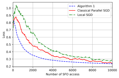
Figure 1: Distributed logistic regression: loss v.s. number of SFO access.

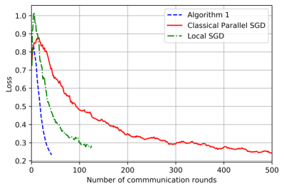
Figure 2: Distributed logistic regression: loss v.s. number of communication rounds.

4.2 Training Deep Neural Networks

Consider using deep learning for the image classification over CIFAR-10 (Krizhevsky & Hinton, 2009). The loss function for deep neural networks is non-convex and typically violates Assumption 2. We run Algorithm 2, the classical parallel SGD, and “local SGD” with communication skipping in (Stich, 2018; Yu et al., 2018) to train ResNet20 (He et al., 2016) with $8$ GPUs. It has been shown that the “local SGD”, also known as parallel restarted SGD or periodic model averaging, can linearly speed up the parallel training of deep neural networks with significantly less communication overhead than the classical parallel SGD (Yu et al., 2018; Lin et al., 2018; Wang & Joshi, 2018; Jiang & Agrawal, 2018). For both parallel SGD and local SGD, the learning rate is $0.1$, the momentum is $0.9$, the weight decay is $1e-4$, and the batch size at each GPU is $32$. For local SGD, we use the largest communication skipping interval for which the loss at convergence does not sacrifice. For Algorithm 2, we use $B_{1}=32$, $\rho=1.02$ and $\gamma=0.1$. In our experiment, each iteration of Algorithm 2 executes CR-PSGD (Algorithm 1) to access one epoch of training data at each GPU. That is, the $T$ parameter in each call of Algorithm 1 is $50000$. The $B_{\tau}$ parameter in Algorithm 1 stop growing when it exceeds $512$.

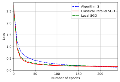
Figure 3: Training deep neural networks: loss v.s. number of SFO access.

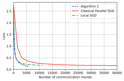
Figure 4: Training deep neural networks: loss v.s. number of communication rounds.

5 Conclusion

In this paper, we explore the idea of using dynamic batch sizes for distributed non-convex optimization. For non-convex optimization satisfying the Polyak-Lojasiewicz (P-L) condition, we show using exponential increasing batch sizes in parallel SGD as in Algorithm 1 can achieve $O(\frac{1}{NT})$ convergence using only $O(\log(T))$ communication rounds. For general stochastic non-convex optimization (without P-L condition), we propose a Catalyst-like algorithm that can achieve $O(\frac{1}{\sqrt{NT}})$ convergence with $O(\sqrt{TN}\log(\frac{T}{N}))$ communication rounds.

6 Supplement

6.1 Basic Facts

This section summarizes several well-known facts for smooth and/or strongly convex functions. For the convenience to the readers, we also provide self-contained proofs to these facts.

Recall that if $\phi({\mathbf{x}})$ is a smooth function with modulus $L>0$, then we have $\phi({\mathbf{y}})\leq\phi({\mathbf{x}})+\langle\nabla\phi({\mathbf{x}}),{\mathbf{y}}-{\mathbf{x}}\rangle+\frac{L}{2}\|{{\mathbf{y}}-{\mathbf{x}}}\|^{2}$ for any ${\mathbf{x}}$ and ${\mathbf{y}}$. This property is known as the descent lemma for smooth functions, see e.g., Proposition A.24 in (Bertsekas, 1999). The next two useful facts follow directly from the descent lemma.

Fact 2.

Let $\phi:{\mathbb{R}}^{m}\mapsto{\mathbb{R}}$ be a smooth function with modulus $L$. If ${\mathbf{x}}^{\ast}$ is a global minimizer of $f$ over ${\mathbb{R}}^{m}$, then

$$\phi({\mathbf{x}})-\phi({\mathbf{x}}^{\ast})\leq\frac{L}{2}\|{{\mathbf{x}}-{\mathbf{x}}^{\ast}}\|^{2},\quad\forall{\mathbf{x}}$$ (24)

Proof.

By the descent lemma for smooth functions, for any ${\mathbf{x}}$, we have

$$\phi({\mathbf{x}})\leq \phi({\mathbf{x}}^{\ast})+\langle\nabla\phi({\mathbf{x}}^{\ast}),{\mathbf{x}}-{\mathbf{x}}^{\ast}\rangle+\frac{L}{2}\|{{\mathbf{x}}-{\mathbf{x}}^{\ast}}\|^{2}$$

$$\overset{(a)}{=} \phi({\mathbf{x}}^{\ast})+\frac{L}{2}\|{{\mathbf{x}}-{\mathbf{x}}^{\ast}}\|^{2}$$

where (a) follows from $\nabla\phi({\mathbf{x}}^{\ast})={\mathbf{0}}$. ∎

Fact 3.

Let $\phi:{\mathbb{R}}^{m}\rightarrow{\mathbb{R}}$ be a smooth function with modulus $L$. We have

$$\frac{1}{2L}\|{\nabla\phi({\mathbf{x}})}\|^{2}\leq\phi({\mathbf{x}})-\phi^{\ast},\quad\forall{\mathbf{x}}$$ (25)

where $\phi^{\ast}$ is the global minimum of $\phi({\mathbf{x}})$.

Proof.

By the descent lemma for smooth functions, for any ${\mathbf{x}},{\mathbf{y}}\in{\mathbb{R}}^{n}$, we have

$$\phi({\mathbf{y}})\leq \phi({\mathbf{x}})+\langle\nabla\phi({\mathbf{x}}),{\mathbf{y}}-{\mathbf{x}}\rangle+\frac{L}{2}\|{{\mathbf{y}}-{\mathbf{x}}}\|^{2}$$

$$\overset{(a)}{=} \phi({\mathbf{x}})+\frac{L}{2}\|{{\mathbf{y}}-{\mathbf{x}}+\frac{1}{L}\nabla\phi({\mathbf{x}})}\|^{2}-\frac{1}{2L}\|{\nabla\phi({\mathbf{x}})}\|^{2}$$

where (a) can be verified by noting that $\|{{\mathbf{y}}-{\mathbf{x}}+\frac{1}{L}\nabla f({\mathbf{x}})}\|^{2}=\|{{\mathbf{y}}-{\mathbf{x}}}\|^{2}+\frac{2}{L}\langle\nabla\phi({\mathbf{x}}),{\mathbf{y}}-{\mathbf{x}}\rangle+\frac{1}{L^{2}}\|{\nabla\phi({\mathbf{x}})}\|^{2}$.

Minimizing both sides over ${\mathbf{y}}\in{\mathbb{R}}^{m}$ yields

$$\phi^{\ast}\leq\phi({\mathbf{x}})-\frac{1}{2L}\|{\nabla\phi({\mathbf{x}})}\|^{2}$$

∎

Recall that if smooth function $\phi({\mathbf{x}})$ is strongly convex with modulus $\mu>0$, then we have $\phi({\mathbf{y}})\geq\phi({\mathbf{x}})+\langle\nabla\phi({\mathbf{x}}),{\mathbf{y}}-{\mathbf{x}}\rangle+\frac{\mu}{2}\|{{\mathbf{y}}-{\mathbf{x}}}\|^{2}$ for any ${\mathbf{x}}$ and ${\mathbf{y}}$. The next two useful facts follow directly from this inequality.

Fact 4.

Let smooth function $\phi:{\mathbb{R}}^{m}\mapsto{\mathbb{R}}$ be strongly convex with modulus $\mu>0$. If ${\mathbf{x}}^{\ast}$ is the (unique) global minimizer of $f$ over ${\mathbb{R}}^{m}$, then

$$\phi({\mathbf{x}})-\phi({\mathbf{x}}^{\ast})\geq\frac{\mu}{2}\|{{\mathbf{x}}-{\mathbf{x}}^{\ast}}\|^{2},\quad\forall{\mathbf{x}}$$ (26)

Proof.

By the strong convexity of $\phi({\mathbf{x}})$, for any ${\mathbf{x}}$, we have

$$\phi({\mathbf{x}})\geq \phi({\mathbf{x}}^{\ast})+\langle\nabla\phi({\mathbf{x}}^{\ast}),{\mathbf{x}}-{\mathbf{x}}^{\ast}\rangle+\frac{\mu}{2}\|{{\mathbf{x}}-{\mathbf{x}}^{\ast}}\|^{2}$$

$$\overset{(a)}{=} \phi({\mathbf{x}}^{\ast})+\frac{\mu}{2}\|{{\mathbf{x}}-{\mathbf{x}}^{\ast}}\|^{2}$$

where (a) follows from $\nabla\phi({\mathbf{x}}^{\ast})={\mathbf{0}}$. ∎

Fact 5.

Let smooth function $\phi:{\mathbb{R}}^{m}\rightarrow{\mathbb{R}}$ be strongly convex with modulus $\mu>0$. If ${\mathbf{x}}^{\ast}$ is the (unique) global minimizer of $\phi({\mathbf{x}})$ over ${\mathbb{R}}^{m}$, then

$$\|{\nabla\phi({\mathbf{x}})}\|\geq\mu\|{{\mathbf{x}}-{\mathbf{x}}^{\ast}}\|,\quad\forall{\mathbf{x}}$$ (27)

Proof.

By Fact 4, we have

$$\phi({\mathbf{x}})-\phi({\mathbf{x}}^{\ast})\geq\frac{\mu}{2}\|{{\mathbf{x}}-{\mathbf{x}}^{\ast}}\|^{2},\quad\forall{\mathbf{x}}$$

By Fact 1 and the definition of P-L condition, we have

$$\frac{1}{2}\|{\nabla\phi({\mathbf{x}})}\|^{2}\geq\mu(\phi({\mathbf{x}})-\phi({\mathbf{x}}^{\ast}),\quad\forall{\mathbf{x}}$$

Combining these two inequalities yields the desired result. ∎

Both Fact 4 and Fact 5 are restricted to strongly convex functions. They can be possibly extended to smooth functions without strong convexity. A generalization of (26) is known as the quadratic growth condition. Similarly, a generalization of (27) is known as the error bound condition. In general, both (26) and (27), where ${\mathbf{x}}^{\ast}$ should be replaced by ${\mathcal{P}}_{\mathcal{X}^{\ast}}[{\mathbf{x}}]$, i.e., the projection of ${\mathbf{x}}$ onto the set of minimizers for $\phi({\mathbf{x}})$ when $\phi({\mathbf{x}})$ does not have a unique minimizer, can be proven to hold as long as smooth $\phi({\mathbf{x}})$ satisfies the P-L condition with the same modulus $\mu$. See Supplement A in (Karimi et al., 2016) for detailed discussions.

6.2 Proof of Theorem 1

Fix $T>1$. Let ${\mathbf{x}}_{t}$ be the solution returned by Algorithm 1 when it terminates. According to the “while” condition in Algorithm 1, we must have $\sum_{\tau=0}^{t-1}\lfloor\rho^{\tau}B_{1}\rfloor\geq T$, which further implies $\sum_{\tau=0}^{t-1}\rho^{\tau}B_{1}\geq T$. Simplifying the partial sum of geometric series and rearranging terms yields

$$t\geq \log_{\rho}\left(\frac{T(\rho-1)}{B_{1}}+1\right)$$

$$\overset{(a)}{\geq} \log_{\rho}\left((\rho-1)\frac{T}{B_{1}}\right)$$

$$= \log_{\frac{1}{\rho}}\left(\frac{B_{1}}{T(\rho-1)}\right)$$ (28)

where (a) follows because $\rho>1$.

By Lemma 1, for all $\tau\in\{1,2,\ldots,t-1\}$, we have

$${\mathbb{E}}[f({\mathbf{x}}_{\tau+1})-f^{\ast}]$$

$$\leq (1-\nu){\mathbb{E}}[f({\mathbf{x}}_{\tau})-f^{\ast}]+\frac{\gamma(2-L\gamma)}{2NB_{\tau}}\sigma^{2}$$

$$\overset{(a)}{\leq} (1-\nu){\mathbb{E}}[f({\mathbf{x}}_{\tau})-f^{\ast}]+\frac{\gamma(2-L\gamma)\sigma^{2}}{NB_{1}}\frac{1}{\rho^{\tau-1}}$$

where (a) follows by recalling $B_{\tau}=\lfloor\rho^{\tau-1}B_{1}\rfloor$ and noting $\lfloor z\rfloor>\frac{1}{2}z$ as long as $z\geq 2$.

Recursively applying the above inequality from $\tau=1$ to $\tau=t-1$ yields

$${\mathbb{E}}[f({\mathbf{x}}_{t})-f^{\ast}]$$

$$\leq (1-\nu)^{t-1}\left(f({\mathbf{x}}_{1})-f^{\ast}\right)+\frac{\gamma(2-L\gamma)\sigma^{2}}{NB_{1}}\sum_{\tau=0}^{t-2}(1-\nu)^{\tau}(\frac{1}{\rho})^{t-2-\tau}$$

$$= (1-\nu)^{t-1}\left(f({\mathbf{x}}_{1})-f^{\ast}\right)+\frac{\gamma(2-L\gamma)\sigma^{2}}{NB_{1}}(\frac{1}{\rho})^{t-2}\sum_{\tau=0}^{t-2}((1-\nu)\rho)^{\tau}$$

$$\overset{(a)}{\leq} (1-\nu)^{t-1}\left(f({\mathbf{x}}_{1})-f^{\ast}\right)+\frac{\gamma(2-L\gamma)\sigma^{2}}{NB_{1}}(\frac{1}{\rho})^{t-2}\frac{1}{1-(1-\nu)\rho}$$

$$\overset{(b)}{\leq} (1-\nu)^{\log_{\frac{1}{\rho}}\left(\frac{B_{1}}{T(\rho-1)}\right)}\frac{1}{1-\nu}\left(f({\mathbf{x}}_{1})-f^{\ast})\right)+\frac{\gamma(2-L\gamma)\sigma^{2}}{N}\frac{1}{1-(1-\nu)\rho}\frac{\rho^{2}}{T(\rho-1)}$$

$$\overset{(c)}{=} \Big{(}\frac{B_{1}}{T(\rho-1)}\Big{)}^{\log_{\frac{1}{\rho}}(1-\nu)}\frac{1}{1-\nu}\left(f({\mathbf{x}}_{1})-f^{\ast}\right)+\frac{\rho^{2}\gamma(2-L\gamma)\sigma^{2}}{(1-(1-\nu)\rho)(\rho-1)}\frac{1}{NT}$$

$$= \frac{1}{1-\nu}\left(f({\mathbf{x}}_{1})-f^{\ast}\right)\Big{(}\frac{B_{1}}{\rho-1}\Big{)}^{\log_{\frac{1}{\rho}}(1-\nu)}\frac{1}{T^{\log_{\frac{1}{\rho}}(1-\nu)}}+\frac{\rho^{2}\gamma(2-L\gamma)\sigma^{2}}{(1-(1-\nu)\rho)(\rho-1)}\frac{1}{NT}$$

$$\overset{(d)}{=} \frac{1}{1-\nu}\left(f({\mathbf{x}}_{1})-f^{\ast}\right)\Big{(}\frac{B_{1}}{\rho-1}\Big{)}^{\log_{\rho}(\frac{1}{1-\nu})}\frac{1}{T^{\log_{\rho}(\frac{1}{1-\nu})}}+\frac{\rho^{2}\gamma(2-L\gamma)\sigma^{2}}{(1-(1-\nu)\rho)(\rho-1)}\frac{1}{NT}$$ (29)

where (a) follows by simplifying the partial sum of geometric series and noting that $(1-\nu)\rho<1$; (b) follows by substituting (28) and noting that $0<1-\nu<1$ and $0<\frac{1}{\rho}<1$; (c) follows by noting that $\log_{\frac{1}{\rho}}\Big{(}\frac{B_{1}}{T(\rho-1)}\Big{)}=\frac{\log_{1-\nu}\big{(}\frac{B_{1}}{T(\rho-1)}\big{)}}{\log_{1-\nu}\big{(}\frac{1}{\rho}\big{)}}=\log_{\frac{1}{\rho}}(1-\nu)\log_{1-\nu}\Big{(}\frac{B_{1}}{T(\rho-1)}\Big{)}=\log_{1-\nu}\Big{(}\Big{(}\frac{B_{1}}{T(\rho-1)}\Big{)}^{\log_{\frac{1}{\rho}}(1-\nu)}\Big{)}$; and (d) follows from $\log_{\frac{1}{\rho}}(1-\nu)=\log_{\rho}(\frac{1}{1-\nu})$.

References

• Bertsekas (1999) Bertsekas, D. P. Nonlinear Programming. Athena Scientific, second edition, 1999.
• Bottou & Bousquet (2008) Bottou, L. and Bousquet, O. The tradeoffs of large scale learning. In Advances in Neural Information Processing Systems (NIPS), 2008.
• Bottou et al. (2018) Bottou, L., Curtis, F. E., and Nocedal, J. Optimization methods for large-scale machine learning. SIAM Review, 60(2):223–311, 2018.
• Davis & Grimmer (2017) Davis, D. and Grimmer, B. Proximally guided stochastic subgradient method for nonsmooth, nonconvex problems. arXiv:1707.03505, 2017.
• De et al. (2017) De, S., Yadav, A., Jacobs, D., and Goldstein, T. Automated inference with adaptive batches. In International Conference on Artificial Intelligence and Statistics (AISTATS), pp.  1504–1513, 2017.
• Dekel et al. (2012) Dekel, O., Gilad-Bachrach, R., Shamir, O., and Xiao, L. Optimal distributed online prediction using mini-batches. Journal of Machine Learning Research, 13(165–202), 2012.
• Devarakonda et al. (2017) Devarakonda, A., Naumov, M., and Garland, M. Adabatch: Adaptive batch sizes for training deep neural networks. arXiv:1712.02029, 2017.
• Friedlander & Schmidt (2012) Friedlander, M. P. and Schmidt, M. Hybrid deterministic-stochastic methods for data fitting. SIAM Journal on Scientific Computing, 34(3):1380–1405, 2012.
• Ghadimi & Lan (2013) Ghadimi, S. and Lan, G. Stochastic first-and zeroth-order methods for nonconvex stochastic programming. SIAM Journal on Optimization, 23(4):2341–2368, 2013.
• Ghadimi et al. (2016) Ghadimi, S., Lan, G., and Zhang, H. Mini-batch stochastic approximation methods for nonconvex stochastic composite optimization. Mathematical Programming, 155(1-2):267–305, 2016.
• Güler (1992) Güler, O. New proximal point algorithms for convex minimization. SIAM Journal on Optimization, 2(4):649–664, 1992.
• Hazan & Kale (2014) Hazan, E. and Kale, S. Beyond the regret minimization barrier: an optimal algorithm for stochastic strongly-convex optimization. Journal of Machine Learning Research, 2014.
• He & Yuan (2012) He, B. and Yuan, X. An accelerated inexact proximal point algorithm for convex minimization. Journal of Optimization Theory and Applications, 154(2):536–548, 2012.
• He et al. (2016) He, K., Zhang, X., Ren, S., and Sun, J. Deep residual learning for image recognition. In IEEE conference on computer vision and pattern recognition (CVPR), 2016.
• Jiang & Agrawal (2018) Jiang, P. and Agrawal, G. A linear speedup analysis of distributed deep learning with sparse and quantized communication. In Advances in Neural Information Processing Systems (NeurIPS), 2018.
• Karimi et al. (2016) Karimi, H., Nutini, J., and Schmidt, M. Linear convergence of gradient and proximal-gradient methods under the Polyak-Lojasiewicz condition. In Joint European Conference on Machine Learning and Knowledge Discovery in Databases, 2016.
• Krizhevsky & Hinton (2009) Krizhevsky, A. and Hinton, G. Learning multiple layers of features from tiny images. Technical report, University of Toronto, 2009.
• Lacoste-Julien et al. (2012) Lacoste-Julien, S., Schmidt, M., and Bach, F. A simpler approach to obtaining an ${O}(1/t)$ convergence rate for the projected stochastic subgradient method. arXiv:1212.2002, 2012.
• Lian et al. (2015) Lian, X., Huang, Y., Li, Y., and Liu, J. Asynchronous parallel stochastic gradient for nonconvex optimization. In Advances in Neural Information Processing Systems (NIPS), 2015.
• Lin et al. (2015) Lin, H., Mairal, J., and Harchaoui, Z. A universal catalyst for first-order optimization. In Advances in Neural Information Processing Systems (NIPS), pp.  3384–3392, 2015.
• Lin et al. (2018) Lin, T., Stich, S. U., and Jaggi, M. Don’t use large mini-batches, use local SGD. arXiv:1808.07217, 2018.
• Nemirovski et al. (2009) Nemirovski, A., Juditsky, A., Lan, G., and Shapiro, A. Robust stochastic approximation approach to stochastic programming. SIAM Journal on optimization, 19(4):1574–1609, 2009.
• Nemirovsky & Yudin (1983) Nemirovsky, A. S. and Yudin, D. B. Problem complexity and method efficiency in optimization. 1983.
• Nesterov (2004) Nesterov, Y. Introductory Lectures on Convex Optimization: A Basic Course. Springer Science & Business Media, 2004.
• Paquette et al. (2018) Paquette, C., Lin, H., Drusvyatskiy, D., Mairal, J., and Harchaoui, Z. Catalyst for gradient-based nonconvex optimization. In International Conference on Artificial Intelligence and Statistics (AISTATS), pp.  1–10, 2018.
• Polyak (1963) Polyak, B. T. Gradient methods for minimizing functionals. Zhurnal Vychislitel’noi Matematikii Matematicheskoi Fiziki, pp.  643–653, 1963.
• Rakhlin et al. (2012) Rakhlin, A., Shamir, O., and Sridharan, K. Making gradient descent optimal for strongly convex stochastic optimization. In Proceedings of International Conference on Machine Learning (ICML), 2012.
• Salzo & Villa (2012) Salzo, S. and Villa, S. Inexact and accelerated proximal point algorithms. Journal of Convex Analysis, 19(4):1167–1192, 2012.
• Smith & Le (2018) Smith, S. L. and Le, Q. V. Understanding generalization and stochastic gradient descent. In Proceedings of the International Conference on Learning Representations (ICLR), 2018.
• Smith et al. (2018) Smith, S. L., Kindermans, P.-J., Ying, C., and Le, Q. V. Don’t decay the learning rate, increase the batch size. In Proceedings of the International Conference on Learning Representations (ICLR), 2018.
• Stich (2018) Stich, S. U. Local SGD converges fast and communicates little. arXiv:1805.09767, 2018.
• Wang & Joshi (2018) Wang, J. and Joshi, G. Cooperative SGD: A unified framework for the design and analysis of communication-efficient SGD algorithms. arXiv:1808.07576, 2018.
• Yu & Neely (2017) Yu, H. and Neely, M. J. A simple parallel algorithm with an ${O}(1/t)$ convergence rate for general convex programs. SIAM Journal on Optimization, 27(2):759–783, 2017.
• Yu et al. (2018) Yu, H., Yang, S., and Zhu, S. Parallel restarted SGD with faster convergence and less communication: Demystifying why model averaging works for deep learning. arXiv:1807.06629, 2018.
• Zhang et al. (2013) Zhang, L., Yang, T., Jin, R., and He, X. ${O}(\log{T})$ projections for stochastic optimization of smooth and strongly convex functions. In International Conference on Machine Learning (ICML), pp. 1121–1129, 2013.