Exact solution of two fluid plasma equations for the creation of jet-like flows and seed magnetic fields in cylindrical geometry

Abstract

An exact solution of two fluid ideal classical plasma equations is presented which shows that the jet-like outflow and magnetic field are generated simultaneously by the density and temperature gradients of both electrons and ions. Particular profiles of density function $\psi=\ln\bar{n}$ (where $\bar{n}$ is normalized by some constant density $N_{0}$) and temperatures $T_{j}$ (for $j=e,i)$ are chosen which reduce the set of nonlinear partial differential equations to two simple linear equations generating longitudinally uniform axial outflow and magnetic field in cylindrical geometry in several astrophysical objects. This mechanism also seems to be operative for producing short scale plasma jets in the solar atmosphere in the form of spicules and flares. The presented solution requires particular profiles of density and temperatures, but it is a natural solution of the two fluid ideal classical plasma equations. Similar jet-like outflows can be generated by the density and temperature gradients in neutral fluids as well.

Key words: astrophysical jets, two fluid plasma outflows, neutral fluid jets, magnetic field generation, baro-clinic vectors

I 1. INTRODUCTION

First observation of astrophysical jets was made long ago cur and later observations showed that jets are collimated outflows of gases and plasmas from a variety of sources ranging from young stellar objects (YSOs) to active galactic nuclei (AGNs) jen ; mes ; fer ; bel . Jets emerging from YSOs have speeds $v$ smaller than speed of light $c$ $(v\leq 10^{-3}c)$ and hence can be treated using classical plasma models while the jets emerging from AGNs have speeds approaching speed of light and are highly relativistic . AGN jets have sizes of the order of $10^{6}pc$ and YSO jets have sizes of the order of $(10^{-4}-1)pc$ . In between these two extremes are the outflows of gases, electron ion plasmas and electron positron plasmas from normal stars, neutron stars, massive X-ray binary systems, galactic stellar mass black holes (or microquasars).

Magnetic fields are considered to be an important constituent of astrophysical jets emerging from accretion disks, compact stars and black holes bla ; con ; fuk . Jets of active galactic nuclei (AGN) are extended up to kilo or mega parsecs with helical magnetic fields chr ; gab1 ; gab2 . The magnetic fields of these objects are generated by large scale currents and are amplified by dynamo effects. Gamma ray bursts are also associated with relativistic plasma outflow. Solar corona has millisions of plasma jets (spicules) and also flares pri ; sal1 ; ste ; haw . The formation of short scale solar spicules and flares seems to be very similar to large scale non-relativistic galactic jets. Cylindrical structures of plasma also emerge in solar corona along with loops and play a role in solar coronal heating.

Theoretical models and numerical studies have been performed to understand the dynamics of relativistic and non-relativistic jets shi ; ouy ; sto ; nak . Non-relativistic simulations for the outflows of plasma from accretion disks have been performed using magnetohydrodynamic (MHD) equations ust ; hon . Simulations using neutral fluid equations have been performed to compare dynamics of relativistic and non-relativistic jets ros . Kelvin-Helmholtz instabilities have also been investigated in supersonic jets in cartesian and cylinrical geometries mic . Plasma jets are also produced in laboratories to understand the physics of jet formation cia ; loe .

Despite a large difference in velocities, scale sizes, luminosities and magnetic energies of the jets emerging from different sources, the physical origin is believed to be very similar. Many physical mechanisms take part in the formation, stability and acceleration of astrophysical jets including rotation, Lorentz force, magnetic field topology, dissipative forces, gravitation and pressure gradients. Extremely large gravitational effects in case of material outflow from massive black holes require general relativity to be invoked. Flows of hot ionized material create currents and Lorentz force.

Observations reveal that in YSOs, some jets rotate in the opposite direction to the rotation of the source i.e. star or disk. Theoretical model has been presented to explain the counter-rotation of astrophysical jets and winds using classical magnetohydrodynamics (MHD) sau . They have shown that the counter rotation is induced by variation of velocity along the flow, or by shocks, or by inhomogeneous magnetic field. They have verified the observed counter-rotation speed both by analytical approach and by computer simulation.

The fundamental source of energy is the thermal energy which is converted into flow and electromagnetic energies in these systems particularly in jets moving with velocities much smaller than speed of light. Our aim is to find out a simple physical mechanism which generates perpendicular jet-like outflows in non-relativistic plasmas and neutral fluids. This means the fundamental source for astrophysical jets is based on thermodynamics coupled with fluid dynamics.

Biermann effect produced by electron baroclinic vector is believed to be the source of seed magnetic fields in stars bie and galaxies laz . It has been pointed out that it is not only the electron baro clinic vector which produces seed magnetic field; rather the ion dynamics is also coupled with the electron dynamics in this mechanism. Hence ions should not be treated as a background of stationary positive charge sal2 ; sal3 . In these studies, cartesian geometry was used and main focus was on the generation of seed magnetic field, therefore an additional assumption was made that magnetic field ${\bf B}$ is related with the vorticity $(\nabla\times{\bf v})$ of plasma as ${\bf B}=\alpha(\nabla\times{\bf v})$ where $\alpha$ was a constant. A theoretical model for the generation of magnetic field in relativistic plasma of early universe has also been presented mah .

The ideal classical MHD equations were solved by decomposing the velocity vector into components in cylindrical geometry to explain counter rotation of jets sau . Then these authors showed that the rotation velocity component can change sign if the velocity of flow along the flux tube becomes smaller than a threshold value. On the other hand, here it is demonstrated that if plasma density and temperatures have particular profiles, then the axial longitudinally uniform flow ${\bf v}$ and magnetic field ${\bf B}$ are created simultaneously. The flow becomes function of density and increases with time. Dissipative terms and gravity are ignored to highlight the physical mechanism and to find out an exact analytical solution of nonlinear partial differential equations. Similarly, it is shown that jet-like flows can also be created in neutral fluids by the density and temperature gradients.

II Two Fluid Plasma Jets

Here it is shown that thermodynamic forces produced by density and temperature gradients of electron and ion fluids create jet-like plasma flows along z-axis in cylindrical geometry. Only electron dynamics is not sufficient to produce such flows; rather it is found that dynamics of ions is coupled with the electrons and hence both positive and negative fluids generate seed magnetic field and plasma flow simultaneously. For the investigation of this long time behavior, electron inertia is ignored $(m_{e}\rightarrow 0)$ and hence momentum conservation yields,

$$0\simeq-en_{e}\left({\bf E}+\frac{1}{c}{\bf v}_{e}\times{\bf B}\right)-\nabla p_{e}$$ (1)

In the limit $\mid\partial_{t}\mid<<\omega_{pe},\Omega_{e},\mid c\nabla\mid$ where $\omega_{pe}=(\frac{4\pi n_{e}e^{2}}{m_{e}})^{\frac{1}{2}}$ is the electron plasma oscillation frequency and $\Omega_{e}=(\frac{eB}{m_{e}c})$ is the electron gyro frequency, Maxwell’s equation reduces to Amperes’ law

$$\nabla\times{\bf B}=\frac{4\pi}{c}{\bf j}$$ (2)

and quasi-neutrality $(n_{e}\simeq n_{i}=n)$ holds. Electron velocity can be defined as,

$${\bf v}_{e}={\bf v}_{i}-\frac{c}{4\pi e}\left(\frac{\nabla\times{\bf B}}{n}\right)$$ (3)

Curl of Eq. (1) yields

$$-\frac{1}{c}\partial_{t}{\bf B}=-\frac{1}{c}\nabla\times({\bf v}_{e}\times{\bf B})-\nabla\times(\frac{\nabla p_{e}}{en})$$ (4)

Using (3) and (4), we obtain

$$\partial_{t}{\bf B}=\nabla\times({\bf v}_{i}\times{\bf B})-(\frac{c}{4\pi ne})\{\nabla\times[(\nabla\times{\bf B})\times{\bf B}]\}$$ (5)

$$+\frac{c}{4\pi ne}\{\nabla\psi\times[(\nabla\times{\bf B})\times{\bf B}]\}-\frac{c}{e}(\nabla\psi\times\nabla T_{e})$$

where $\psi=\ln\bar{n}$, $\bar{n}=\frac{n}{N_{0}}$ and $N_{0}$ is arbitrary constant density. Curl of ion equation of motion

$$(\partial_{t}+{\bf v}_{i}\cdot\nabla){\bf v}_{i}=en\left({\bf E}+\frac{1}{c}{\bf v}_{i}\times{\bf B}\right)-\nabla p_{i}$$ (6)

yields,

$$a\partial_{t}{\bf B}+\partial_{t}(\nabla\times{\bf v}_{i})=\nabla\times[{\bf v}_{i}\times(\nabla\times{\bf v}_{i})]+a\nabla\times({\bf v}_{i}\times{\bf B})+\frac{1}{m_{i}}(\nabla\psi\times\nabla T_{i})$$ (7)

where $a=\frac{e}{m_{i}c}$. Ideal gas law $p_{j}=n_{j}T_{j}$ has been used for both electron and ion fluids where $j=e,i$. Let us assume longitudinally uniform flow by imposing the condition $\nabla\cdot{\bf v}_{j}=0$ and hence density does not vary with time i.e. $\partial_{t}n=0$. The continuity equations

$$\partial_{t}n+n\nabla\cdot{\bf v}_{j}+\nabla n\cdot{\bf v}_{j}=0$$ (8)

demand

$$\nabla\psi\cdot{\bf v}_{j}=0$$ (9)

which due to (3) also requires,

$$\nabla\psi\cdot(\nabla\times{\bf B})=0$$ (10)

Let the plasma density vary in $(r,\theta)$-plane and temperatures be functions of $z$ coordinate only, viz,

$$\psi=\psi(r,\theta)$$ (11)

and

$$T_{j}=-T_{j}^{\prime}z=-(\frac{T_{j0}}{\delta_{j}})z$$ (12)

where $T_{j}^{\prime}$ is constant and it denotes derivative of $T_{j}$ with respect to $z$ and $\delta_{j}$ is the scale length of the temperature gradient. Equations (11) and (12) yield,

$$\nabla\psi=(\partial_{z}\psi){\bf e}_{r}+(\frac{1}{r}\partial_{\theta}\psi){\bf e}_{\theta}$$ (13)

and

$$\nabla T_{j}=-\frac{T_{j}}{\delta_{j}}{\bf e}_{z}$$ (14)

Here ${\bf e}_{r}$,${\bf e}_{z}$, and ${\bf e}_{\theta}$ are unit vectors along radial, axial and angular directions, respectively. Note that when $\psi=0$, we have $n=N_{0}$. Using equations (11-14), we find

$$(\nabla\psi\times\nabla T_{e})=(-\frac{T_{e0}}{r}\partial_{\theta}\psi){\bf e}_{r}+(\frac{T_{e0}}{\delta_{e}}\partial_{r}\psi){\bf e}_{\theta}$$ (15)

and

$$(\nabla\psi\times\nabla T_{i})=(-\frac{T_{i0}}{r}\partial_{\theta}\psi){\bf e}_{r}+(\frac{T_{i0}}{\delta_{i}}\partial_{r}\psi){\bf e}_{\theta}$$ (16)

Gradient of $\psi$ in $(r,\theta)$-plane along with the condition (10) forces ${\bf B}$ to have the following form of spatial dependence,

$${\bf B}=(\nabla\chi(r,\theta)\times{\bf e}_{z})=\frac{1}{r}(\partial_{\theta}\chi){\bf e}_{r}+(-\partial_{r}\chi){\bf e}_{\theta}$$ (17)

which yields,

$$\nabla\times{\bf B}=-\nabla^{2}\chi(r,\theta){\bf e}_{z}$$ (18)

Note that the vector potential ${\bf A}$ has only $z$-component non-zero i.e. ${\bf A}=A_{z}{\bf e}_{z}=\chi{\bf e}_{z}$ and hence the magnetic helicity H is zero, viz,

$$\emph{H}={\bf A}\cdot{\bf B}=0$$ (19)

Our aim is to show that time-independent forms of density and temperature gradients are able to create time-dependent jet-like flows in the axial direction perpendicular to $(r,\theta)$-plane. Now we prove that following form of plasma axial flow is created by the above mentioned profiles of $\nabla\psi$ and $\nabla T_{j}$,

$${\bf v}_{i}=u(r,\theta)f(t){\bf e}_{z}$$ (20)

It will be seen later that plasma flow in axial direction becomes a function of density and temperature. The nonlinear terms of electron and ion fluid equations can be expressed in terms of scalars defined above as follows,

$$\nabla\times({\bf v}_{i}\times{\bf B})=\{u,\chi\}f(t){\bf e}_{z}$$ (21)

$$\nabla\times[(\nabla\times{\bf B})\times{\bf B}]=\{\chi,\nabla^{2}\chi\}{\bf e}_{z}$$ (22)

and

$$\nabla\psi\times[(\nabla\times{\bf B})\times{\bf B}]=[\{\chi,\psi\}\nabla^{2}\chi]{\bf e}_{z}$$ (23)

where

$$\{f,g\}=\frac{1}{r}(\partial_{r}f\partial_{\theta}g-\partial_{\theta}f,\partial_{r}g)$$ (24)

Note that

$$\nabla\times[{\bf v}_{i}\times(\nabla\times{\bf v}_{i})]=0$$ (25)

Let us impose the following conditions on density, magnetic field and flow,

$$\{\chi,\psi\}=\{u,\chi\}=0=\{\chi,\nabla^{2}\chi\}=0$$ (26)

Interestingly under these conditions all the nonlinear terms of Eqs.(5) and (7) vanish and they reduce, respectively, to

$$\partial_{t}{\bf B}=-\frac{c}{e}(\nabla\psi\times\nabla T_{e})$$ (27)

and

$$a\partial_{t}{\bf B}+\partial_{t}(\nabla\times{\bf v}_{i})=\frac{1}{m_{i}}(\nabla\psi\times\nabla T_{i})$$ (28)

Due to (20), we have

$$\nabla\times{\bf v}_{i}=\{(\frac{1}{r}\partial_{\theta}u){\bf e}_{r}-(\partial_{r}u){\bf e}_{\theta}\}f(t)$$ (29)

therefore ion vorticity (29), baroclinic vectors (15,16) and magnetic field (17) all become parallel to each other. Using (20) and (13) in equations (27) and (28), we obtain

$$\partial_{t}\chi=\frac{cT_{e0}^{\prime}}{e}\psi$$ (30)

and

$$u\partial_{t}f=-(\frac{T_{e0}^{\prime}+T_{i0}^{\prime}}{m_{i}})\psi$$ (31)

Let $\chi=h(r,\theta)f(t)$ and integrate (30) and (31) for $t:0\rightarrow\tau$ to get, respectively,

$$\chi(r,\theta,\tau)=h(r,\theta)f(\tau)=\frac{cT_{e0}^{\prime}}{e}\psi(r,\theta)\tau$$ (32)

and

$$v_{i}(r,\theta,\tau)=u(r,\theta)f(\tau)=-(\frac{T_{e0}^{\prime}+T_{i0}^{\prime}}{m_{i}})\psi(r,\theta)\tau$$ (33)

Since $u=u(\psi)$ and $\chi=\chi(\psi)$, therefore $\{\chi,\psi\}=0$ and $\{u,\chi\}=0$ hold. Note that $f(t)=(constant)t$ has been assumed.

Now we try to find out an exact solution of the nonlinear two fluid plasma equations by choosing an appropriate form of $\psi$ which fulfills all the above assumptions. For this, we impose a condition on $\psi$, such that

$$\nabla^{2}\psi=-\lambda^{2}\psi$$ (34)

where $\lambda$ is a constant. Following relations of Bessel functions hold,

$$\frac{dJ_{1}(\lambda r)}{dr}=\lambda J_{0}(\lambda r)-\frac{1}{r}J_{1}(\lambda r)$$ (35)

and

$$\frac{d^{2}J_{1}(\lambda r)}{dr^{2}}=-(\frac{2\lambda^{2}}{r^{2}})J_{1}(\lambda r)-\frac{\lambda}{r}J_{0}(\lambda r)$$ (36)

where $J_{0}$ and $J_{1}$ are Bessel functions of order zero and one, respectively. The magnetic field $\chi$ and plasma flow $u$ have been expressed in terms of density function $\psi$ in equations (30) and (31). Let us define,

$$\psi(r,\theta)=\psi_{0}J_{1}(\lambda r)\cos(\theta)$$ (37)

where $\psi_{0}$ is the magnitude of $\psi$ and $\lambda$ is the scale length of density variation. With this definition of $\psi$ the condition $\{\chi,\nabla^{2}\chi\}=0$ mentioned in (26) also holds. Density function $\psi$ approaches zero for large $\lambda r$. The form of this function is illustrated in Fig. (1). Flow and magnetic field have also similar forms but the direction of flow is axial and it increases with time. Since all physical quantities vary like $J_{1}$ therefore this solution is valid in the limited region of the source where $\psi$ has the given form. At large $\lambda r$ the density becomes equal to the background density, say $n_{0}$ and phenomenon disappears.

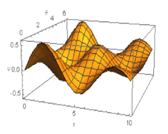
Figure 1: Density function $\psi=\ln\bar{n}$ is plotted vs $\lambda r:0\rightarrow 10$ and $\theta:0\rightarrow 2\pi$. Similar axial flow ${\bf v}$ out of plasma disc is created and it increases with time because it is directly proportional to $\psi$ and $t$.

It is very interesting to note that the form of density function given in (37) fulfills all the above conditions. Thus an exact solution of two fluid plasma equations (5) and (7) exists in cylindrical geometry which predicts that both magnetic field and ion vorticity are generated simultaneously by the baro clinic vectors of electrons and ions. Plasma is ejected in the z-direction like a jet perpendicular to $(r,\theta)$ plane. Velocity $u$ becomes zero where $J_{1}=0$ or $\cos\theta=0$. Strictly speaking these are the points where flow disappears. This means the flow under this theoretical model is broken in pieces. At these points the density becomes equal to background density.

III Neutral Fluid Jets

In this section, we show that neutral fluid is also ejected out of a two dimensional material spread in $(r,\theta)$ plane in the form of a jet along $z$-axis in the cylindrical geometry. Let us consider an ideal neutral fluid with density $\rho$, velocity ${\bf v}$ and pressure $p$. Its dynamics is governed by the following two simple equations,

$$\rho(\partial_{t}+{\bf v}\cdot\nabla){\bf v}=-\nabla p$$ (38)

and

$$\partial_{t}n+\nabla\cdot(n{\bf v})=0$$ (39)

where $\rho=mn$ and $m$ is mass of the fluid particle. We again assume longitudinally uniform flow $\nabla\cdot{\bf v}=0$ with time independent density i.e. $\partial_{t}\rho=0$. Then the continuity equation demands $\nabla n\cdot{\bf v}=0$ which can be expressed as

$$\nabla\psi\cdot{\bf v}=0$$ (40)

where $\psi=\ln{\bar{n}}$ and $\bar{n}=\frac{n}{N_{0}}$ and $N_{0}$ is constant density at axis of the cylinder $(r=0)$. Curl of equation (38) gives,

$$\partial_{t}(\nabla\times{\bf v})=\nabla\times[{\bf v}\times(\nabla\times{\bf v})]+\frac{1}{m}(\nabla\psi\times\nabla T)$$ (41)

If nonlinear term vanishes

$$\nabla\times\{{\bf v}\times(\nabla\times{\bf v})\}=0$$ (42)

then we obtain a simpler equation for the vorticity generation

$$\partial_{t}(\nabla\times{\bf v})=\frac{1}{m}(\nabla\psi\times\nabla T)$$ (43)

This shows that vorticity can be generated in the neutral fluid by the baro clinic vector. If this is true, then we need to find out a suitable solution which satisfies the conditions (40) and (42) along with equation (43). Let us consider density and temperature profiles as follows,

$$\psi=\psi(r,\theta)$$ (44)

and

$$T=-T_{0}^{\prime}z=-\frac{T}{\delta}z$$ (45)

which give,

$$\nabla\psi=(\partial_{t}\psi){\bf e}_{r}+(\frac{1}{r}\partial_{\theta}\psi){\bf e}_{\theta}$$ (46)

and

$$\nabla T=-T_{0}^{\prime}{\bf e}_{z}=-\frac{T}{\delta}{\bf e}_{z}$$ (47)

where $T_{0}^{\prime}=\frac{T_{0}}{\delta_{0}}$ is a constant, $\delta_{0}$ is temperature gradient scale length and $\hat{z}$ is unit vector along axis of the cylinder. Equations (46) and (47) yield,

$$(\nabla\psi\times\nabla T)=-T_{0}^{\prime}\left[(\frac{1}{r}\partial_{\theta}\psi){\bf e}_{r}+(-\partial_{r}\psi){\bf e}_{\theta}\right]$$ (48)

Equation (43) shows that vorticity is parallel to $(\nabla\psi\times\nabla T)$, hence we choose the form of flow as,

$${\bf v}=u(r,\theta)f(t){\bf e}_{z}$$ (49)

Then (43) can be expressed as,

$$\{(\frac{1}{r}\partial_{\theta}u){\bf e}_{r}+(-\partial_{r}u){\bf e}_{\theta}\}\partial_{t}f=-\frac{T_{0}^{\prime}}{m}\{(\frac{1}{r}\partial_{\theta}\psi){\bf e}_{r}+(-\partial_{r}\psi){\bf e}_{\theta}\}$$ (50)

Integrating for $t=0\rightarrow\tau$, it yields,

$$\{(\frac{1}{r}\partial_{\theta}u){\bf e}_{r}+(-\partial_{r}u){\bf e}_{\theta}\}\partial_{t}f=-\frac{T_{0}^{\prime}}{m}\{(\frac{1}{r}\partial_{\theta}\psi){\bf e}_{r}+(-\partial_{r}\psi){\bf e}_{\theta}\}\tau$$ (51)

Equation (50) gives a relation between flow $u$ and density $\psi$ as

$$u(r,\theta)=-\frac{T_{0}^{\prime}}{m}\psi(r,\theta)$$ (52)

where

$$f(t)=(constant)t$$ (53)

Now we try to choose a particular form of $\psi$ which should satisfy all the above mentioned assumptions. Let

$$\psi=\psi_{0}J_{1}(\lambda r)\cos\theta$$ (54)

The density at $r=0$ is constant $N_{0}$ and hence ${\bf v}=0$ at the axis. However, vorticity $(\nabla\times{\bf v})$ will have several zeros in $(r,\theta)$-plane because this plane is expanded along $r$. Then we find

$$u(r,\theta)=-\frac{T_{0}^{\prime}}{m}\psi_{0}J_{1}(\mu r)\cos\theta$$ (55)

Equation (52) shows that neutral material is ejected in the form of jet along $z$-axis out of two dimensional density structure while the temperature gradient is along the direction of flow.

IV Discussion

Keeping in view the long time plasma behavior, a formulism has been presented in which all the physical quantities turn out to be the functions of density $\psi$ chosen in Eq. (37). Interestingly, all the nonlinear terms vanish naturally and hence all the assumptions used to derive the simple linear equations (27) and (28) are satisfied. Solution of these equations under the condition (34) is given by Eq.(37). Here $\psi_{0}$ is the amplitude and $\psi$ varies along radial direction like Bessel function of order one $(J_{1})$ and in $\theta$-direction the variation is chosen to be like $\cos\theta$. This form of density function reduces the set of nonlinear partial differential equations to two linear equations. It seems important to mention here that the presented solution requires particular profiles of density and temperatures, but it is a natural solution of the two fluid classical plasma equations which predicts the creation of jet-like plasma outflow ${\bf v}_{(r,\theta)}$ and the magnetic field ${\bf B}_{(r,\theta)}$ simultaneously. Unlike self-gravitating systems ben , we just focus attention on the investigation of outflows from a plasma and a fluid source (star or a disc) and do not include additional forces like gravity.

First we have considered a two fluid classical ideal plasma to show that the driving force for the observed astrophysical and laboratory jets is based on the structures of density and temperature gradients. This theoretical model suggests that magnetic field and plasma outflow are produced simultaneously in astrophysical objects and they evolve with time from a non-equilibrium $(T_{e}\neq T_{i})$ two fluid ideal classical plasma. Important point to note is that the highly nonlinear system of two fluid plasma equations can create an ordered structure in the form of a jet. The driving force of such flows and associated magnetic fields is produced by the thermodynamic free energy available in the form of density and temperature gradients. Similar mechanism in classical plasma in the Sun’s atmosphere seems to be operative for producing short scale plasma jets in millions (the spicules) and solar flares as well as cylindrical plasma structures in solar corona.

Second, it has also been shown that jet-like outflows are also created in neutral fluids by the same physical mechanism. Here it has also been found that the baro clinic vector of a neutral fluid produces jet like structures expelling the material in the axial direction. Thus density and temperature gradients seem to be the fundamental source of jet formation in both neutral fluids and classical plasma systems.

The Fig. (1) illustrates the profile of $\psi$ for the range of $\lambda r:0\rightarrow 10$ and $\theta:0\rightarrow 2\pi$. Equation (33) gives the form of axial flow as a function of $\psi$ but increasing with time because flow is directly proportional to time $t$. Similar flow can be created in neutral fluids as well. Thus axial flows can be created by density and temperature gradients in both neutral fluids and plasmas.

- (1) H. Curtis, Publ. Lick Obs. 13, 31 (1918).
- (2) R.C. Jennison and M.K. Das Gupta, Nature 172, 996 (1953).
- (3) L. Mestel, L. Mon.Not. R. Astron. Soc. 122, 473 (1961).
- (4) A. Ferrari, Annu. Rev. Astron. Astrophys. 36, 539 (1998).
- (5) P.M. Bellan, Phys. Plasmas 25, 055601 (2018).
- (6) R.D. Blandford and D.G. Payne, Mon. Not. R. Astron. Soc., 199, 883 (1982).
- (7) J. Contopoulos and R.V.E. Lovelace, Asptrophys. J. 429, 139 (1994).
- (8) K. Fukumura, D. Kazana, C. Schrader, E. Behar, F. Tombesi, and I. Contopoulos, Nat. Astron. 2017, 1, 62 (2017).
- (9) D.M. Christodoulou, D.C. Gabuzda, S. Knuettel, I. Contopoulos, D. Kazanas, and C.P. Coughlan, Astron. Astrophys. 2016, 591, 61 (2016).
- (10) D.C. Gabuzda, S. Knuettel, B. Reardon, Mon. Not. R. Astron. Soc. 450, 2441 (2015).
- (11) D.C. Gabuzda, N. Roche, A. Kirwan, S. Kneuttel, M. Nagle, and C. Houston, Mon. Not. R. Astron. Soc. 472, 1792 (2017).
- (12) E.R. Priest, Solar Magnetohydrodynamics (Dordrecht: Reidel, 1982)
- (13) H. Saleem, J. Vranjes, and Poedts, S. Astron. Astrophys. 471, 289 (2007).
- (14) E.V. Stenson, and P.M. Bellan, Phys. Rev. Lett. 109, 075001 (2012).
- (15) M.A. Haw and P.M. Bellan, Geophys. Res. Lett. 44, 9525 (2017).
- (16) K. Shibata and Y. Uchida, Sol. Phys. 103, 299 (1986).
- (17) R. Ouyed and R.E. Pudritz, Astrophys. J. 482, 712 (1997)
- (18) J.M. Stone and P.E. Hardee, Astrophys. J. 540, 192 (2000).
- (19) M. Nakamura, D. Garofalo, and D.L. Meier, Astrophys. J. 721, 1783 (2010).
- (20) G.V. Ustyugova, A.V. Koldoba, M.M. Romanova, V.M. Chechetkin, and R.V.E. Lovelace, Astrophys. J. 439, L39 (1995).
- (21) M. Honda and Y.S. Honda, Astrophys. J. 569, L39 (2002).
- (22) A. Rosen, P.A. Hughes, G.C. Duncan, and P.E. Hardee, Astrophys. j. 516, 729 (1999).
- (23) M. Micono, S. Massaglia, G. Bodo, P. Rossi, and A. Ferrari, Astron. Astrophys. 333, 989 (1998).
- (24) A. Ciardi, S.V. Lebedev, A. Frank, F. Suzuki-Vidal, G.N. Hall, S.N. Bland, A. Harvey-Thompson, E.G. Blackman, and M. Camenzind, Astrophys. J. 691, L147 (2009).
- (25) K.T.K. Loebner, T.C. Underwood, T. Mouratidis, and M.A. Cappelli, Appl. Phys. Lett. 108, 094104 (2016).
- (26) Sauty, C., Cayatte, V., Lima, J.J.G., Matsakos, T., and Tsinganos, K. 2012, Astrophys. J. Lett. 759, L1.
- (27) L. Biermann, Z. Naturforsch. B 5A, 65 (1950).
- (28) A. Lazarian, Astron. Astrophys. 264, 326 (1992).
- (29) H. Saleem and Z. Yoshida, Phys. Plasmas 11, 4865 (2004).
- (30) H. Saleem, Phys. Plasmas 17, 092101 (2010).
- (31) S.M. Mahajan and Z. Yoshida, Phy. Rev. Lett. 105, 095005 (2010).
- (32) D. Benhaiem, F.S. Labini, and J. Michael, Phys. Rev. E 99, 022125 (2019).