Spectral Reconstruction with Deep Neural Networks

Abstract

We explore artificial neural networks as a tool for the reconstruction of spectral functions from imaginary time Green’s functions, a classic ill-conditioned inverse problem. Our ansatz is based on a supervised learning framework in which prior knowledge is encoded in the training data and the inverse transformation manifold is explicitly parametrised through a neural network. We systematically investigate this novel reconstruction approach, providing a detailed analysis of its performance on physically motivated mock data, and compare it to established methods of Bayesian inference. The reconstruction accuracy is found to be at least comparable, and potentially superior in particular at larger noise levels. We argue that the use of labelled training data in a supervised setting and the freedom in defining an optimisation objective are inherent advantages of the present approach and may lead to significant improvements over state-of-the-art methods in the future. Potential directions for further research are discussed in detail.

I Introduction

Machine Learning has been applied to a variety of problems in the natural sciences. For example, it is regularly deployed in the interpretation of data from high-energy physics detectors [1, 2]. Algorithms based on learning have shown to be highly versatile, with their use extending far beyond the original design purpose. In particular, deep neural networks have demonstrated unprecedented levels of prediction and generalisation performance, for reviews see e.g. [3, 4]. Machine Learning architectures are also increasingly deployed for a variety of problems in the theoretical physics community, ranging from the identification of phases and order parameters to the acceleration of lattice simulations [5, 6, 7, 8, 9, 10, 11, 12, 13, 14, 15, 16].

Ill-conditioned inverse problems lie at the heart of some of the most challenging tasks in modern theoretical physics. One pertinent example is the computation of real-time properties of strongly correlated quantum systems. Take e.g. the phenomenon of energy and charge transport, which so far has defied a quantitative understanding from first principles. This universal phenomenon is relevant to systems at vastly different energy scales, ranging from ultracold quantum gases created with optical traps to the quark-gluon plasma born out of relativistic heavy-ion collisions.

While static properties of strongly correlated quantum systems are by now well understood and routinely computed from first principles, a similar understanding of real-time properties is still subject to ongoing research. The thermodynamics of strongly coupled systems, such as the quark gluon plasma, has been explored using the combined strength of different non-perturbative approaches, such as functional renormalisation group methods and lattice field theory calculations. There are two limitations affecting most of these approaches: Firstly, in order to carry out quantitative computations, time has to be analytically continued into the complex plane, to so-called Euclidean time. Secondly, explicit computations are either fully numerical or at least involve intermediate numerical steps.

This leaves us with the need to eventually undo the analytic continuation of Euclidean correlation functions, which are known only approximately. The most relevant examples are two-point functions, the so-called Euclidean propagators. The spectral representation of quantum field theory relates the propagators, be they in Minkowski or Euclidean time, to a single function encoding their physics, the so-called spectral function. The number of different structures contributing to a spectral function are in general quite limited and consist of poles and cuts. If we can extract from the Euclidean two-point correlator its spectral function, we may immediately compute the corresponding real-time propagator.

If we know the Euclidean propagator analytically, this information allows us in principle to recover the corresponding Minkowski time information. In practice, however, the limitation of having to approximate correlator data (e.g. through simulations) turns the computation of spectral functions into an ill-conditioned problem. The most common approach to give meaning to such inverse problems is Bayesian inference. It incorporates additional prior domain knowledge we possess on the shape of the spectral function to regularise the inversion task. The positivity of hadronic spectral functions is one prominent example. The Bayesian approach has seen continuous improvement over the past two decades in the context of spectral function reconstructions. While originally it was restricted to maximum a posteriori estimates for the most probable spectral function given Euclidean data and prior information [17, 18, 19], in its most modern form it amounts to exploring the full posterior distribution [20]. An important aspect of the work is to develop appropriate mock data tests to benchmark the reconstruction performance before applying it to actual data. Generally, the success of a reconstruction method stands or falls with its performance on physical data. While this seems evident, it was in fact a hard lesson learned in the history of Bayesian reconstruction methods, a lesson which we want to heed.

Inverse problems of this type have also drawn quite some attention in the machine learning (ML) community [21, 22, 23, 24]. In the present work we build upon both the recent progress in the field of ML, particularly deep learning, as well as results and structural information gathered in the past decades from Bayesian reconstruction methods. We set out to isolate a property of neural networks that holds the potential to improve upon the standard Bayesian methods, while retaining their advantages, utilising the already gathered insight in their study.

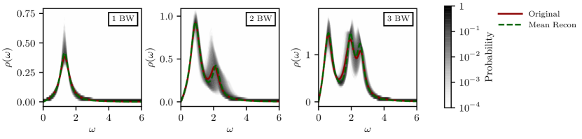
Figure 1: Examples of mock spectral functions reconstructed via our neural network approach for the cases of one, two and three Breit-Wigner peaks. The chosen functions mirror the desired locality of suggested reconstructions around the original function (red line). Additive, Gaussian noise of width $10^{-3}$ is added to the discretised analytic form of the associated propagator of the same original spectral function multiple times. The shaded area depicts for each frequency $\omega$ the distribution of resulting outcomes, while the dashed green line corresponds to the mean. The results are obtained from the FC parameter network optimised with the parameter loss. The network is trained on the largest defined parameter space which corresponds to the volume Vol O. The uncertainty for reconstructions decreases for smaller volumes as illustrated in Figure 4. A detailed discussion on the properties and problems of a neural network based reconstruction is given in Section IV.1.

Consider a feed-forward deep neural network that takes Euclidean propagator data as input and outputs a prediction of the associated spectral function. Although the reasoning behind this ansatz is rather different, one can draw parallels to more traditional methods. In the Bayesian approach, prior information is explicitly encoded in a prior probability functional and the optimisation objective is the precise recovery of the given propagator data from the predicted spectral function. In contrast, the neural network based reconstruction is conditioned through supervised learning with appropriate training data. This corresponds to implicitly imposing a prior distribution on the set of possible predictions, which, as in the Bayesian case, regularises the reconstruction problem. Optimisation objectives are now expressed in terms of loss functions, allowing for greater flexibility. In fact, we can explicitly provide pairs of correlator and spectral function data during the training. Hence, not only can we aim for the recovery of the input data from the predictions as in the Bayesian approach, but we are now also able to formulate a loss directly on the spectral functions themselves. This constitutes a much stronger restriction on potential solutions for individual propagators, which could provide a significant advantage over other methods. The possibility to access all information of a given sample with respect to its different representations also allows the exploration of a much broader set of loss functions, which could benefit not only the neural network based reconstruction, but also lead to a better understanding and circumvention of obstacles related to the inverse problem itself. Such an obstacle is given, for example, by the varying severity of the problem within the space of considered spectral functions. By employing adaptive losses, inhomogeneities of this type could be neutralised.

Similar approaches concerning spectral functions that consist of normalised sums of Gaussian peaks have already been discussed in [25, 26]. In this work, we investigate the performance of such an approach using mock data of physical resonances motivated by quantum field theory, and compare it to state-of-the-art Bayesian methods. The data are given in the form of linear combinations of unnormalised Breit-Wigner peaks, whose distinctive tail structures introduce additional difficulties (see Figure 1 for an example reconstruction). Using only a rather naive implementation, the performance of our ansatz is demonstrated to be at least comparable and potentially superior, particularly for large noise levels. We then discuss potential improvements of the architecture, which in the future could establish neural networks to a state-of-the-art approach for accurate reconstructions with a reliable estimation of errors.

The paper is organised as follows. The spectral reconstruction problem is defined in Section II.1. State-of-the-art Bayesian reconstruction methods are summarised in Section II.2. In Section II.3 we discuss the application of neural networks and potential advantages. Section III contains details on the design of the networks and defines the optimisation procedure. Numerical results are presented and compared to Bayesian methods in Section IV. We summarise our findings and discuss future work in Section V.

II Spectral reconstruction and potential advantages

II.1 Defining the problem

Typically, correlation functions in equilibrium quantum field theories are computed in imaginary time after a Wick rotation $t\to it\equiv\tau$, which facilitates both analytical and numerical computations. In strongly correlated systems, a numerical treatment is in most cases inevitable. Such a setup leaves us with the task to reconstruct relevant information, such as the spectrum of the theory, or genuine real-time quantities such as transport coefficients, from the Euclidean data.

The information we want to access is encoded in the associated spectral function $\rho$. For this purpose it is most convenient to work in momentum space both for $\rho$ and the corresponding propagator $G$. The relation between the Euclidean propagator and the spectral function is given by the well known Källen-Lehmann spectral representation,

$$G(p) =\int_{0}^{\infty}\frac{\mathrm{d}\omega}{\pi}\frac{\omega\,\rho(\omega)}{\omega^{2}+p^{2}}\equiv\int_{0}^{\infty}\mathrm{d}\omega\,K(p,\omega)\rho(\omega)\,,$$ (1)

which defines the corresponding Källen-Lehmann kernel. The propagator is usually only available in the form of numerical data, with finite statistical and systematic uncertainties, on a discrete set of $N_{p}$ points, which we abbreviate as $G_{i}=G(p_{i})$. The most commonly used approach is to work directly with a discretised version of 1. We utilise the same abbreviation for the spectral function, i.e. $\rho_{i}=\rho(\omega_{i})$, discretised on $N_{\omega}$ points. This lets us state the discrete form of 1 as

$$G_{i}=\sum_{j=1}^{N_{\omega}}K_{ij}\,\rho_{j}\,\,,$$ (2)

where $K_{ij}=K(p_{i},\omega_{j})\Delta\omega_{j}$. This amounts to a classic ill-conditioned inverse problem, similar in nature to those encountered in many other fields, such as medical imaging or the calibration of option pricing methods. Typical errors on the input data $G(p_{i})$ are on the order of $10^{-2}$ to $10^{-5}$ when the propagator at zero momentum is of the order of unity.

To appreciate the problems arising in such a reconstruction more clearly, let us assume we have a suggestion for the spectral function $\rho_{\text{\tiny{sug}}}$ and its corresponding propagator $G_{\text{\tiny{sug}}}$. The difference to the measured data is encoded in

$$\|G(p)- G_{\text{\tiny{sug}}}(p)\|=$$

$$\bigg{\|}\int_{0}^{\infty}\frac{\mathrm{d}\omega}{\pi}\frac{\omega}{\omega^{2}+p^{2}}\,\Big{[}\rho(\omega)-\rho_{\text{\tiny{sug}}}(\omega)\Big{]}\bigg{\|}\,,$$ (3)

with a suitable norm $\|.\|$. Evidently, even if this expression vanishes point-wise, i.e. $\|G(p_{i})-G_{\text{\tiny{sug}}}(p_{i})\|=0$ for all $p_{i}$, the spectral function is not uniquely fixed. Experience has shown that with typical numerical errors on the input data, qualitatively very different spectral functions can lead to in this sense equivalent propagators. This situation can often be improved on by taking more prior knowledge into account, c.f. the discussion in [27]. This includes properties such as:

1. Normalisation and positivity of spectral functions of asymptotic states. For gauge theories, this may reduce to just the normalisation to zero, expressed in terms of the Oehme-Zimmermann superconvergence [28, 29].

2. Asymptotic behaviour of the spectral function at low and high frequencies.

3. The absence of clearly unphysical features, such as drastic oscillations in the spectral function and the propagator.

Additionally, the parametrisation of the spectral function in terms of frequency bins is just one particular basis. In order to make reconstructions more feasible, other choices, and in particular physically motivated ones, may be beneficial, c.f. again the discussion in [27]. In this work, we consider a basis formulated in terms of physical resonances, i.e. Breit-Wigner peaks.

II.2 Existing methods

The inverse problem as defined in 1 has an exact solution in the case of exactly known, discrete correlator data [30]. However, as soon as noisy inputs are considered, this approach turns out to be impractical [31]. Therefore, the most common strategy to treat this problem is via Bayesian inference. This approach is based on Bayes’ theorem, which states that the posterior probability is essentially given by two terms, the likelihood function and prior probability:

$$P(\rho|D,I)\propto P(D|\rho,I)\,P(\rho|I)\,.$$ (4)

It explicitly includes additionally available prior information on the spectral function in order to regularise the inversion task. The likelihood $P(D|\rho)$ encodes the probability for the input data $D$ to have arisen from the test spectral function $\rho$, while $P(\rho)$ quantifies how well this test function agrees with the available prior information. The two probabilities fully specify the posterior distribution in principle, however they may be known only implicitly. In order to gain access to the full distribution, one may sample from the posterior, e.g. through a Markov Chain Monte Carlo process in the parameter space of the spectral function. However, in practice one is often content with the maximum a posteriori (MAP) solution. Given a uniform prior, the Maximum Likelihood Estimate (MLE) corresponds to an estimate of the MAP.

II.3 Advantages of neural networks

In order to make genuine progress, we set out in this study to explore methods in which our prior knowledge of the analytic structure can be encoded in different ways. To this end, our focus lies on the use of Machine Learning in the form of artificial neural networks. These feature a high flexibility in the encoding of information by learning abstract internal representation. They possess the advantageous properties that prior information can be explicitly provided through the training data, and that the solution space can be regularised by choosing appropriate loss functions.

Minimising II.1, while respecting the constraints discussed in Section II.1, can be formulated as minimising the propagator loss

$$L_{G}(\rho_{\text{\tiny{sug}}}) =\lVert G[\rho_{\text{\tiny{sug}}}]-G[\rho]\rVert\,.$$ (5)

This corresponds to indirectly working on a norm or loss function for $\rho$, the spectral function loss

$$L_{\rho}(\rho_{\text{\tiny{sug}}})=\lVert\rho_{\text{\tiny{sug}}}-\rho\rVert\,.$$ (6)

Of course, the optimisation problem as given by 6 is intractable, since it requires the knowledge of the true spectral function $\rho$. Minimising $L_{\rho}(\rho_{\text{\tiny{sug}}})$ for a given set of $\{\rho_{\text{\tiny{sug}}}\}$ also minimises $L_{G}$, since the Källén–Lehmann representation 1 is a linear map. In turn, however, minimising $L_{G}$ does not uniquely determine the spectral function, as has already been mentioned. Accordingly, the key to optimise the spectral reconstruction is the ideal use of all known constraints on $\rho$, in order to better condition the problem. The latter aspect has fueled many developments in the area of spectral reconstructions in the past decades.

Given the complexity of the problem, as well as the interrelation of the constraints, this calls, in our opinion, for an application of supervised machine learning algorithms for an optimal utilisation of constraints. To demonstrate our reasoning, we generate a training set of known pairs of spectral functions and propagators and train a neural network to reconstruct $\rho$ from $G$ by minimising a suitable norm, utilising both $L_{G}$ and $L_{\rho}$ during the training. When the network has converged, it can be applied to measured propagator data $G$ for which the corresponding $\rho$ is unknown.

Estimators learning from labelled data provide a potentially significant advantage due to the employed supervision, because the loss function is minimised a priori for a whole range of possible input/output pairs. Accordingly, a neural network aims to learn the entire set of inverse transformations for a given set of spectral functions. After this mapping has been approximated to a sufficient degree, the network can be used to make predictions. This is in contrast to standard Bayesian methods, where the posterior distribution is explored on a case by case basis. Both approaches may also be combined, e.g. by employing a neural network to suggest a solution $\rho_{sug}$, which is then further optimised using a traditional algorithm.

The given setup forces the network to regularise the ill-conditioned problem by reproducing the correct training spectrum in accord with our criteria for a successful reconstruction. It is the inclusion of the training data and the free choice of loss functions that allows the network to fully absorb all relevant prior information. This ability is an outstanding property of supervised learning methods, which could yield potentially significant improvements over existing frameworks. for such constraints are the analytic structure of the propagator, asymptotic behaviors and normalisation constraints.

The parametrisation of an infinite set or manifold of inverse transformations by the neural network also enables the discovery of new loss functions which may be more appropriate for a reliable reconstruction. This includes, for example, the exploration of correlation matrices with adapted elements, in order to define a suitable norm for the given and suggested propagators. Existing, iterative methods may also benefit from the application of such adaptive loss functions. These may include parameters, point-like representations and arbitrary other characteristics of a given training sample.

Formulated in a Bayesian language, we set out to explicitly train the neural network to predict MAP estimates for each possible input propagator, given the training data as prior information. By salting the input data with noise, the network learns to return a denoised representation of the associated spectral functions.

III A neural network based reconstruction

Neural networks provide high flexibility with regard to their structure and the information they can process. They are capable of learning complex internal representations which allow them to extract the relevant features from a given input. A variety of network architectures and loss functions can be implemented in a straightforward manner using modern Machine Learning frameworks. Prior information can be explicitly provided through a systematic selection of the training data. The data itself provides, in addition to the loss function, a regularisation of possible suggestions. Accordingly, the proposed solutions have the advantage to be similar to the ones in the training data.

The section starts with notes on the design of the neural networks we employ and ends with a detailed introduction of the training procedure and the utilised loss functions.

III.1 Design of the neural networks

Figure 2: Sketch of our strategy for reconstructing (a) the parameters using the PaNet and (b) the discretised data points using the PoNet (and by extension also the PoNetVar). Details on the architectures are given in Appendix C.

We construct two different types of deep feed-forward neural networks. The input layer is fed with the noisy propagator data $G(p)$. The output for the first type is an estimate of the parameters of the associated $\rho$ in the chosen basis, which we denote as parameter net (PaNet). For the second type, the network is trained directly on the discretised representation of the spectral function. This network will be referred to as point net (PoNet). A consideration of a variable number of Breit-Wigners is feasible per construction by the point-like representation of the spectral function within the output layer. This kind of network will in the following be abbreviated by PoNetVar. See Figure 2 for a schematic illustration of our strategy. Note that in all cases a basis for the spectral function is provided either explicitly through the structure of the network or implicitly through the choice of the training data. If not stated otherwise, the numerical results presented in the following always correspond to results from the PaNet.

We compare the performance of fully-connected (FC) and convolutional (Conv) layers as well as the impact of their depth and width. In general, choosing the numbers of layers and neurons is a trade-off between the expressive power of the network, the available memory and the issue of overfitting. The latter strongly depends on the number of available training samples w.r.t. the expressivity. For fully parametrised spectral functions, new samples can be generated very efficiently for each training epoch, which implies an, in principle, infinite supply of data. Therefore, in this case, the risk of overfitting is practically non-existent. The specific dimensions and hyperparameters used for this work are provided in Appendix C. Numerical results can be found in Section IV.

III.2 Training strategy

The neural network is trained with appropriately labelled input data in a supervised manner. This approach allows to implicitly impose a prior distribution in the Bayesian sense. The challenge lies in constructing a training dataset that is exhaustive enough to contain the relevant structures that may constitute the actual spectral functions in practical applications.

From our past experience with hadronic spectral functions in lattice QCD and the functional renormalisation group, the most relevant structures are peaks of the Breit-Wigner type, as well as thresholds. The former present a challenge from the point of view of inverse problems, as they contain significant tail contributions, contrary e.g. to Gaussian peaks, which approach zero exponentially fast. Thresholds on the other hand set in at finite frequencies, often involving a non-analytic kink behavior. In this work, we only consider Breit-Wigner type structures as a first step for the application of neural networks to this family of problems.

Mock spectral functions are constructed using a superposed collection of Breit-Wigner peaks based on a parametrisation obtained directly from one-loop perturbative quantum field theory. Each individual Breit-Wigner is given by

$$\rho^{(\tiny{BW})}(\omega)=\frac{4A\Gamma\omega}{(M^{2}+\Gamma^{2}-\omega^{2})^{2}+4\Gamma^{2}\omega^{2}}\,.$$ (7)

Here, $M$ denotes the mass of the corresponding state, $\Gamma$ its width and $A$ amounts to a positive normalisation constant.

Spectral functions for the training and test set are constructed from a combination of at most $N_{\textnormal{BW}}=3$ different Breit-Wigner peaks. Depending on which type of network is considered, the Euclidean propagator is obtained either by inserting the discretised spectral function into 2, or by a computation of the propagator’s analytic representation from the given parameters. The propagators are salted both for the training and test set with additive, Gaussian noise

$$G_{i}^{\rm noisy}=G_{i}+\epsilon\,.$$ (8)

This is a generic choice which allows to quantify the performance of our method at different noise levels.

The advantage of neural networks to have direct access to different representations of a spectral function implies a free choice of objective functions in the solution space. We consider three simple loss functions and combinations thereof. The (pure) propagator loss $L_{G}(\rho_{\text{\tiny{sug}}})$ defined in 5 represents the most straightforward approach. This objective function is accessible also in already existing frameworks, such as Bayesian Reconstruction (BR) or Hamiltonian Monte Carlo (HMC) methods, in particular the GrHMC framework (referring to the retarded propagator $G_{r}$) developed in [27]. It is implemented in this work to facilitate a quantitative comparison. In contrast, the loss functions that follow are only accessible in the neural network based reconstruction framework. This unique property is owed to the possibility that a neural network can be trained in advance on a dataset of known input and output pairs. As pointed out in Section II.3, a loss function can e.g. be defined directly on a discretised representation of the spectral function $\rho$. This approach is implemented through $L_{\rho}(\rho_{\text{\tiny{sug}}})$, see 6. The optimisation of the parameters $\theta=\{A_{i},M_{i},\Gamma_{i}\,|\,0\leq i<N_{\textnormal{BW}}\}$ of our chosen basis is an even more direct approach. In principle, the space of all possible choices of parameters is $\mathbb{R}_{+}^{3\cdot N_{BW}}$, assuming they are all positive definite. Of course, only finite subvolumes of this space ever need to be considered as target spaces for reconstruction methods. Therefore, we will often refer to a finite target volume simply as the parameter space for a specific setting. Accordingly, in addition to the propagator and spectral function losses defined in Equations 5 and 6, the respective parameter loss in this space is given by:

$$L_{\theta}(\theta_{\text{\tiny{sug}}})=\lVert\theta_{\text{\tiny{sug}}}-\theta\rVert\,.$$ (9)

All losses are evaluated using the 2-norm. In the case of the parameter net, we have $\rho_{\text{\tiny{sug}}}\equiv\rho(\theta_{\text{\tiny{sug}}})$. Apart from the three given loss functions, we also investigate a combination of the propagator and the spectral function loss,

$$L_{G,\rho}(\rho_{\text{\tiny{sug}}},\alpha)=L_{\rho}(\rho_{\text{\tiny{sug}}})+\alpha L_{G}(\rho_{\text{\tiny{sug}}})\,,$$ (10)

where the parameter $\alpha$ determines the relative importance of the two losses. In our experiments, we have chosen it such as to roughly balance differences in the scales of the respective loss functions. The type of loss function that is employed as well as the selection of the training data have major impact on the resulting performance of the neural network. Given this observation, it seems likely that a further optimisation regarding the choice of the loss function can significantly enhance the prediction quality. However, for the time being, we content ourselves with the types given above and postpone the exploration of more suitable training objectives to future work.

IV Numerical results

In this section we present numerical results for the neural network based reconstruction and validate the discussed potential advantages by comparing to existing methods. Details on the training procedure as well as the training and test datasets can be found in Table 1 and Appendix C, together with an introduction to the used performance measures. We start now with a brief summary of the main findings for our approach. Furthermore, a detailed numerical analysis and discussion of different network setups w.r.t performance differences are provided. Subsequently, additional post-processing methods for an improvement of the neural network predictions are covered. The section ends with a discussion of results from the PoNet. Readers who are interested in a comparison of the neural network based reconstruction to existing methods may proceed directly with Section IV.2.

IV.1 Reconstruction with neural networks

Figure 3: The performance of different net architectures and loss functions of a parameter net is compared for additive Gaussian noise with widths of $10^{-3}$ and $10^{-5}$ on the given input propagator: (a) Comparison of different net architecures. All networks are trained based on the parameter loss. The associated architectures can be found in Table 3. (b) Comparison of different loss functions. Details on the loss functions are described at the end of Section III.2. All results are based on networks with the architecture Conv. To (a) and (b): Shown here are the respective losses for the predicted parameters, for the discretised reconstructed spectral function and for the reconstructed propagator to the true, noise-free propagator. Both figures use the largest volume in parameter space, Vol O. The definitions of the performance measures are given at the end of Appendix C. The results on the left hand side imply that for larger errors, the choice of a specific network architecture has negligible impact on the quality of the reconstructions. All performance measures can be lowered for the given noise widths by applying a post-processing procedure on the suggested parameters of the network. In particular, the propagator loss can be minimised. The comparison on the right hand side shows that the choice of the loss function has major impact on the resulting performance of the network. The results underpin the importance of an appropriate loss function and support our argument of potential advantages of neural networks compared to existing approaches in Section II.3. Contour plots in parameter space are illustrated for the respective measures in Figure 12 and Figure 13.

Our findings concerning the optimal setup of a feed-forward network can be summarised as follows. As pointed out in Section II.3, the network aims to learn an approximate parametrisation of a manifold of (matrix) inverses of the discretised Källén-Lehmann transformations. The inverse problem grows more severe if the propagator values are afflicted with noise. In Bayesian terms, this is caused by a wider posterior distribution for larger noise. The network needs to have sufficient expressivity, i.e. an adequate number of hyperparameters, to be able to learn a large enough set of inverse transformations. We assume that for larger noise widths a smaller number of hyperparameters is necessary to learn satisfactory transformations, since the available information content about the actual inverse transformation decreases for a respective exact reconstruction. A varying severity of the inverse problem within the parameter space leads to an optimisation of the spectral reconstruction in regions where the problem is less severe. This effect occurs naturally, since there the network can minimise the loss more easily than in regions where the problem is more severe. Besides the severity of the inverse problem, the form of the loss function has a large impact on global optima within the landscape of the solution space. Based on these observations, an appropriate training of the network is non-trivial and demands a careful numerical analysis of the inverse problem itself, and of different setups of the optimisation procedure. A sensible definition of the loss function or a non-uniform selection of the training data are possible approaches to address the disparity in the severity of the inverse problem. A more straightforward approach is to iteratively reduce the covered parameter ranges within the learning process, based on previous suggested outcomes. This amounts to successively increasing the prediction accuracy by restricting the network to smaller and smaller subvolumes of the original solution space. However, one should be aware that this approach is only sensible if the reconstructions for different noise samples on the original propagator data are sufficiently close to each other in the solution space. A successive optimisation of the prediction accuracy in such a way can also be applied to existing methods. All approaches ultimately aim at a more homogeneous reconstruction loss within the solution space. This allows for a reliable control of systematic errors, as well as an accurate estimation of statistical errors. The desired outcome for a generic set of Breit-Wigner parameters is illustrated and discussed in Figure 1.

The quality and reliability of reconstructions heavily depend on the following details of the training procedure and the inverse problem itself, with varying levels of impact given a specific situation:

• local differences in the severity of the inverse problem

• information loss in the forward pass and due to statistical noise

• loss function / prior information

• complexity / expressivity of the network architecture

In essence, we wish to emphasise that a reliable reconstruction is a multifactorial problem whose facets need to be disentangled in order to understand all contributions to systematic errors.

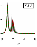
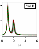
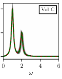
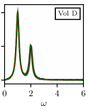
Figure 4: The uncertainties of reconstructions of spectral functions on the same original propagator are illustrated in the same manner as described in Figure 1 for different volumes of the parameter space, again using a noise width of $10^{-3}$. The plots demonstrate how the quality of the reconstruction improves if the parameter space which the network has to learn is decreased. The volumes of the corresponding parameter spaces are listed in Table 1. The results are computed from the Conv PaNet. The systematic deviation of the distribution of reconstructions for large volumes shows that the network has not captured the manifold of inverse transformations completely for the entire parameter space. This is in concordance with the results discussed in Figure 12 and Figure 14.

Figure 5: The plots in this figure quantify the impact of the parameter space volume used for the training on the performance of the parameter network. The performance measures are computed based on the test set of the smallest volume, Vol D. The parameter ranges in the training set are gradually reduced to analyse different levels of complexity of the problem. Separate networks are trained for each volume, which are listed in Table 1. The results demonstrate the potential advantage of an iterative restriction of the parameter ranges of possible solutions. The contour plots in Figure 14 depict changes of the performance measures within the parameter space. More strongly peaked prior distributions lead to better reconstructions. The comparison with results of the GrHMC approach illustrates the improvement of the performance of neural networks for larger errors and smaller volumes. These observations confirm the discussions of Figure 4 and Figure 8. Adding a post-processing step leads in particular for the propagator loss and for smaller noise widths to an improvement of the reconstruction, as has also been discussed in Figure 3.

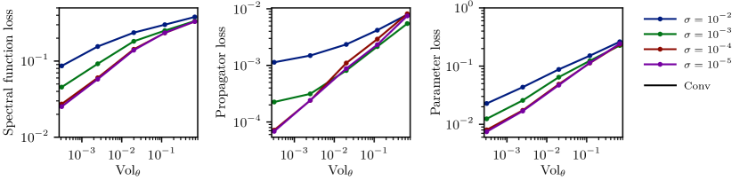
Figure 6: Comparison of reconstruction errors of the Conv PaNet trained only on the smallest Vol D for different noise levels, evaluated with test volumes which are also larger than D. The test datasets are equivalent to the ones used for the other tasks described in this paper. In contrast to Figure 5, which shows the prediction quality as a function of the training volume with a fixed test volume Vol D, here the performance is evaluated as a function of the test volume using a fixed training volume.

Figure 7: Comparison of reconstruction errors of the PaNet and the PoNet for the FC architecture. The performance measures are computed based on the test set of the largest parameter space volume Vol O for one, two and three Breit-Wigners. All networks are trained based on the parameter ranges of Vol O. Loss functions are the parameter loss $L_{\theta}$ for the PaNet and the spectral function loss $L_{\rho}$ for both PoNets. The overall smaller losses for the point nets are due to the large number of degrees of freedom for the point-like representation of the spectral function. The partly competitive performance of the PoNetVar compared to the results of the PoNet encourage the further investigation of networks that are trained using a more exhaustive set of basis functions to describe physical structures in the spectral functions.

The impact of the net architecture and the loss function on the overall performance within the parameter space is illustrated in Figure 3. Associated contour plots can be found in the appendix, Figures 12 and 13. These plots demonstrate that the minima in the loss landscape highly depend on the employed loss function. In turn, this leads to different performance measures. This observation confirms our previous discussion and the necessity of an appropriate definition of the loss function. It also reinforces our arguments regarding potential advantages of neural networks in comparison to other approaches for spectral reconstruction. The comparison of different feed-forward network architectures shows that the specific details of the network structure are rather irrelevant, provided that the expressivity is sufficient.

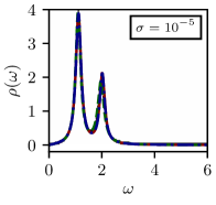
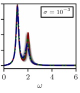
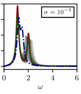
Figure 8: The quality of the reconstruction of two Breit-Wigner peaks is compared for different strength of additive noise on the same propagator. The labels indicate the noise width on the original propagator. It can be seen that the reconstructed spectral function of the neural network exhibits in particular for larger errors a lower deviation to the original spectral function than the GrHMC method. This mirrors the in general observable better performance of the neural network for larger errors, as can be seen in Figure 5 and in Figure 9. The green and the red curve correspond to reconstructions of the Conv PaNet and the GrHMC method for the same given noisy propagator. The prior is in both cases given by the parameter range of volume Vol B. The uncertainty of the reconstructions for the neural network is depicted by the grey shaded areas as described in Figure 1. For small errors, this area is covered by the corresponding reconstructed spectral functions.

Figure 9: The performance of the reconstruction of spectral functions is benchmarked for the parameter network, which is trained with $L_{\theta}$, by a comparison to results of the GrHMC method. The parameter network is in particular for large noise widths competitive. The worse performance for smaller noise widths is a result of an inappropriate training procedure and a too low expressive power of the neural network. The problems are caused by a varying severity of the inverse problem and by a too large parameter space that needs to be covered by the neural network, as discussed in Section IV.1. The error bars of the results for the FC network are representative for typical errors within all methods and plots of this kind.

Differences in the performance of the networks that are trained with the same loss function become less visible for larger noise. This is illustrated by a comparison of contour plots with different noise widths, see e.g. Figure 12. The severity of the inverse problem grows with the noise and the information content about the actual matrix transformation decreases. These properties lead to the observation of a generally worse performance for larger noise widths, as can be inferred from Figure 4, as well as Figures 8 and 9, which are discussed later. They also imply that for specific noise widths, the neural network possesses enough hyperparameters to learn a sufficient parametrisation of the inverse transformation manifold. Furthermore, the local optima into which the network converges are mainly determined by differences in the local severity of the inverse problem. Hence, the issue remains that generic loss functions are inappropriate to address the varying local severity of the inverse problem. This issue implies the existence of systematic errors for particular regions within the parameter space, as can be seen e.g. in the left plot of Figure 4.

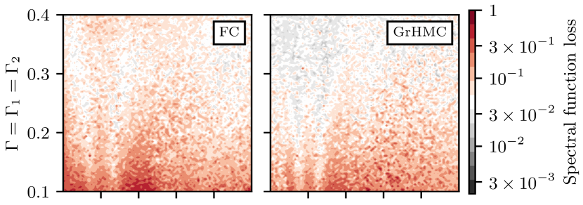
Figure 10: Comparison of performance measures for the reconstruction of two Breit-Wigners of the FC parameter network with the GrHMC method for input propagators with noise width $10^{-3}$ within the parameter space volume Vol O. The similar loss landscape emphasises the high impact of variations of the severity of the inverse problem within the parameter space on the quality of reconstructions. Contrary to expectations, the parameter network mimics, despite an optimisation based on the parameter loss $L_{\theta}$, the reconstruction of the GrHMC method which relies on an optimisation of the propagator loss $L_{G}$ with respect to the parameters. A reconstruction resulting in an averaged peak with the other parameter set effectively removed, as outlined in [27], results in the spiking parameter losses for the GrHMC reconstructions with large errors.

Vol	A	M	$\Gamma$	$\Delta M$
O	$[0.1,1.0]$	$[0.5,3.0]$	$[0.1,0.4]$	$[0.0,2.5]$
A	$[0.3,0.7]$	$[0.5,3.0]$	$[0.1,0.3]$	$[0.25,1.75]$
B	$[0.4,0.6]$	$[0.5,3.0]$	$[0.1,0.2]$	$[0.5,1.5]$
C	$[0.45,0.55]$	$[0.5,3.0]$	$[0.1,0.15]$	$[0.75,1.25]$
D	$[0.475,0.525]$	$[0.5,3.0]$	$[0.1125,0.1375]$	$[0.875,1.125]$

Table 1: Parameter ranges of the different volumes in parameter space used for training. Parameters are sampled uniformly based on the given bounds for the training and test sets. For the case of two and three Breit-Wigner functions, the difference in mass $\Delta M=M_{2}-M_{1}$ is limited to restrict the minimum possible distance between two peaks. The volumes $V_{\theta}$ are computed based on these parameter ranges.

The results shown in Figures 4 and 5 as well as Figure 14 in the appendix confirm our discussion regarding the expressive power of the network w.r.t. the complexity of the solution space and the decreasing information content for larger errors. The parameter space is gradually reduced, effectively increasing the expressivity of the network relative to the severity of the problem and improving the behavior of the loss function for a given fixed parameter space. The respective volumes are listed in Table 1. Shrinking the parameter space leads to a more homogeneous loss landscape due to the increased locality, thereby mitigating the issue of inappropriate loss functions. The necessary number of hyperparameters decreases for larger noise widths and smaller parameter ranges in the training and test dataset. The arguments above imply a better performance of the network for smaller parameter spaces. A reduction of the parameter space effectively corresponds to a sharpening of the prior information, which also has positive effects on the spread of the posterior distribution. More detailed discussions on the impact of different elements of the training procedure can be found in the captions of the respective figures.

Since increasing the expressivity of the network is limited by the computational demand required for the training, one can also apply post-processing methods to improve the suggested outcome w.r.t. the initially given, noisy propagator. These methods are motivated by the in some cases large observed root-mean-square deviation of the reconstructed suggested propagator to the input, see for example again Figure 3. The application of standard optimisation methods on the suggested results of the network represents one possible approach to address this problem. Here, the network’s prediction is interpreted as a guess of the MAP estimate, which is presumed to be close to the true solution. For the PaNet, we minimise the propagator loss a posteriori with respect to the following loss function:

$$\min_{\theta_{\text{\tiny{sug}}}}\;L_{\textnormal{PP}}[\theta_{\text{\tiny{sug}}}]=\min_{\theta_{\text{\tiny{sug}}}}\;\lVert G_{\textnormal{noisy}}-G\left[\rho\left(\theta_{\text{\tiny{sug}}}\right)\right]\rVert\,.$$ (11)

This ensures that suggestions for the reconstructed spectral functions are in concordance with the given input propagator. Results obtained with an additional post-processing are marked by the attachment PP in this work. The numerical results in Figures 4 and 9 show that the finite size of the neural network can be partially compensated for small errors. The resulting low propagator losses are noteworthy, and are close to state-of-the-art spectral reconstruction approaches. One reason for this similarity is the shared underlying objective function. However, the situation is different for larger noise widths. For our choice of hyperparameters, the algorithm quickly converges into a local minimum. For large noise widths, the optimisation procedure may even lead to worse results than the initially suggested reconstruction. This is due to the already mentioned systematic deviations which are caused by the inappropriate choice of the loss function for large parameter spaces. This kind of post-processing should therefore be applied with caution, since it may cancel out the potential advantages of neural networks w.r.t. the freedom in the definition of the loss function.

The following alternative post-processing approach preserves the potential advantages of neural networks while nevertheless minimising the propagator loss. The idea is to include the network into the optimisation process through the following objective:

$$\min_{G_{\textnormal{input}}}\;L_{\textnormal{input}}[G_{\textnormal{input}}]=\min_{G_{\textnormal{input}}}\;\lVert G_{\textnormal{noisy}}-G\left[\rho\left(\theta_{\text{\tiny{sug}}}\right)\right]\rVert\,,$$ (12)

where $G_{\textnormal{input}}$ corresponds to the input propagator of the neural network and $\theta_{\text{\tiny{sug}}}$ to the associated outcome. This facilitates a compensation of badly distributed noise samples and allows a more accurate error estimation. The approach is only sensible if no systematic errors exist for reconstructions within the parameter space, and if the network’s suggestions are already somewhat reliable. We postpone a numerical analysis of this optimisation method together with the exploration of more appropriate loss functions and improved training strategies to future work, due to a currently lacking setup to train such a network.

Figure 11: Reconstructions of one, two and three Breit-Wigners are compared for our proposed neural network approach, the GrHMC method and the BR method. The reconstructions of the first two methods are based on a single sample with noise width $10^{-3}$, while the results of the BR method are obtained from multiple samples with larger errors, but an average noise width of $10^{-3}$ as well. In contrast to the previous plots, the neural network and the GrHMC method now use different priors for each case in order to allow for a reasonable comparison with the BR method, see Table 2. We observe that all approaches qualitatively capture the features in the spectral function. Due to the comparably large error on the input data, all methods are expected to face difficulties in finding an accurate solution. The reconstructions of the neural network approach and the GrHMC method are comparable, whereas the BR method struggles in particular with thin peaks and the three Breit-Wigner case. The results demonstrate that, generally, using suitable basis functions and incorporating prior information lead to a superior reconstruction performance.

Figures 6 and 15 serve to quantify the generalization capability of our neural network approach with regard to data that lie outside of the training volume. Figure 6 shows a comparison of error metrics obtained with the Conv PaNet trained only on the smallest Vol D when applied to larger parameter volumes, at a few different noise levels. As we expect, the performance decreases with larger test volumes, but loss values notably remain in the same orders of magnitude that are observed for larger training volumes, indicating that the generalization capability of the network has at first only a rather weak dependence on the ratio between test and training volume, which only grows more severe if the test volume becomes much larger. This is further illustrated by Figure 15, showing a rather flat loss landscape in the immediate vicinity of the training volume boundaries without sharp transitions, and gradual worsening of the prediction quality as one moves further away. We conclude that our approach is moderately robust against deviations of the true solution from the considered training volume and only fails at larger distances.

In Figures 7 and 16, results of the PoNet and the PaNet are compared. We observe that spectral reconstructions based on the PoNet structure suffer from similar problems as the PaNet. The point-like representation of the spectral function introduces a large number of degrees of freedom for the solution space. The training procedure implicitly regularises this problem, however, a visual analysis of individual reconstructions shows that in some cases the network struggles with common issues known from existing methods, such as partly non-Breit-Wigner like structures and wiggles. An application of the proposed post-processing methods serves as a possible approach to circumvent such problems. An inclusion of further regulator terms into the loss function, concerning e.g. the smoothness of the reconstruction, is also possible.

IV.2 Benchmarking and discussion

In this section, we want to emphasise differences of our proposed neural network approach to existing methods. Our arguments are supported by an in-depth numerical comparison.

Within all approaches the aim is to map out, or at least to find the maximum of, the posterior distribution $P(\rho|G)$ for a given noisy propagator $G$. The BR and GrHMC methods represent iterative approaches to accomplish this goal. The algorithms are designed to find the maximum for each propagator on a case-by-case basis. The GrHMC method additionally provides the possibility to implement constraints on the functional basis of the spectral function in a straightforward manner. In contrast, a neural network aims to learn the full manifold of inverse Källen-Lehman transformations for any noisy propagator (at least within the chosen parameter space). In this sense, it needs to propose for each given propagator an estimate of the maximum of $P(\rho|D)$. A complex parametrisation, as given by the network, an exhaustive training dataset and the optimisation procedure itself are essential features of this approach for tackling this tough challenge. The computational effort to find a solution in an iterative approach is therefore shifted to the training process as well as the memory demand of the network. Accordingly, the neural network based reconstruction can be performed much faster after training has been completed, which is in particular advantageous when large sets of input propagators are considered. In our experiments, the time required for running the GrHMC algorithm and training the networks was roughly similar, generally being of the order of a few hours. A quantitative comparison is difficult due to the use of completely distinct software packages and different utilisation of hardware accelerators. However, we emphasise again that one run of the GrHMC can only provide a prediction for one specific propagator, whereas the trained network can be evaluated quickly on large datasets and additionally allows fast retraining when different data are expected, without having to start from scratch.

The numerical results in Figures 5, 8, 9, 10 and 11 demonstrate that the formal arguments of Section II.3 apply, particularly for comparably large noise widths as well as smaller parameter ranges. For both cases, the network successfully approximates the required inverse transformation manifold. Smaller noise widths and a larger set of possible spectral functions can be addressed by increasing the number of hyperparameters and through the exploration of more appropriate loss functions, as was already discussed previously.

V Conclusion

In this study we have explored artificial neural networks as a tool to deal with the ill-conditioned inverse problem of reconstructing spectral functions from noisy Euclidean propagator data. We systematically investigated the performance of this approach on physically motivated mock data and compared our results with existing methods. Our findings demonstrate the importance of understanding the implications of the inverse problem itself on the optimisation procedure as well as on the resulting predictions.

The crucial advantage of the presented ansatz is the superior flexibility in the choice of the objective function. As a result, it can outperform state-of-the-art methods if the network is trained appropriately and exhibits sufficient expressivity to approximate the inverse transformation manifold. The numerical results demonstrate that defining an appropriate loss function grows increasingly important for an increased variability of considered spectral functions and of the severity of the inverse problem.

In future work, we aim to further exploit the advantage of neural networks that local variations in the severity of the inverse problem can be systematically compensated. The goal is to eliminate systematic errors in the predictions in order to facilitate a reliable reconstruction with an accurate error estimation. This can be realised by finding more appropriate loss functions with the help of implicit and explicit approaches [32, 33]. A utilisation of these loss functions in existing methods is also possible if they are directly accessible. Varying the prior distribution will also be investigated, by sampling non-uniformly over the parameter space during the creation of the training data. Furthermore, we aim at a better understanding of the posterior distribution through the application of invertible neural networks [24]. This novel architecture provides a reliable estimation of errors by mapping out the entire posterior distribution by construction.

In conclusion, we believe that the suggested improvements will boost the performance of the proposed method to an as of yet unprecedented level and that neural networks will eventually replace existing state-of-the-art methods for spectral reconstruction.

Appendix A BR method

Different Bayesian methods propose different prior probabilities, i.e. they encode different types of prior information. The well-known Maximum Entropy Method e.g. features the Shannon-Jaynes entropy

$$S_{\rm SJ}=\int d\omega\big{(}\rho(\omega)-m(\omega)-\rho(\omega){\rm log}\big{[}\frac{\rho(\omega)}{m(\omega)}\big{]}\big{)},$$ (13)

while the more recent BR method uses a variant of the gamma distribution

$$S_{\rm BR}=\int d\omega\big{(}1-\frac{\rho(\omega)}{m(\omega)}+{\rm log}\big{[}\frac{\rho(\omega)}{m(\omega)}\big{]}\big{)}.$$ (14)

Both methods e.g. encode the fact that physical spectral functions are necessarily positive definite but are otherwise based on different assumptions.

As Bayesian methods they have in common that the prior information has to be encoded in the functional form of the regulator and the supplied default model $m(\omega)$. Note that discretising $\rho$ by choosing a particular functional basis also introduces a selection of possible outcomes. The dependence of the most probable spectral function, given input data and prior information, on the choice of $S$, $m(\omega)$ and the discretised basis comprises the systematic uncertainty of the method.

One major limitation to Bayesian approaches is the need to formulate our prior knowledge in the form of an optimisation functional. The reason is that while many of the correlation functions relevant in theoretical physics have very well defined analytic properties it has not been possible to formulate these as a closed regulator functional $S$. Take as an example the retarded propagator (for a more comprehensive discussion see [27]). Its analytic structure in the imaginary frequency plane splits into two parts, an analytic half-plane, where the Euclidean input data is located, and a meromorphic half-plane which contains all structures contributing to the real-time dynamics. Encoding this information in an appropriate regulator functional has not yet been achieved.

Instead the MEM and the BR method rather use concepts unspecific to the analytic structure, such as smoothness, to derive their regulators. Among others this e.g. manifests itself in the presence of artificial ringing, which is related to unphysical poles contributing to the real-time propagator, which however should be suppressed by a regulator functional aware of the physical analytic properties.

Appendix B GrHMC method

The main idea of the setup is already stated in the main text in Section II and was first introduced in [27]. Nevertheless, for completeness we outline the entire reconstruction process here. The approach is based on formulating the basis expansion in terms of the retarded propagator. The resulting set of basis coefficients are then determined via Bayesian inference. This leaves us with two objects to specify in the reconstruction process, the choice of a basis/ansatz for the retarded propagator and suitable priors for the inference.

Once a basis has been chosen it is straightforward to write down the corresponding regression model. As in the reconstruction with neural nets we use a fixed number of Breit-Wigner structures, c.f. 7, corresponding to simple poles in the analytically continued retarded propagator. The logarithm of all parameters is used in the model in order to enforce positivity of all parameters. The uniqueness of the parameters is ensured by using an ordered representation of the logarithmic mass parameters.

The other crucial point is the choice of priors, which are of great importance to tame the ill-conditioning practically and should therefore be chosen as restrictive as possible. For comparability to the neural net reconstruction, the priors are matched to the training volume in parameter space. However, it is more convenient to work with a continuous distribution. Hence the priors of the logarithmic parameters are chosen as normal distributions where we have fixed the parameters by the condition that the mean of the distribution is the mean of the training volume and the probability at the boundaries of the trainings volume is equal. Details on the training volume in parameter space can be found in Table 1 and Appendix C.

All calculations for the GrHMC method are carried out using the python interface [34] of Stan [35].

Appendix C Mock data, training set and training procedure

We consider three different levels of difficulty for the reconstruction of spectral functions to analyse and compare the performance of the approaches in this work. These levels differ by the number of Breit-Wigners that need to be extracted based on the given information of the propagator. We distinguish between training and test sets with one, two and three Breit-Wigners. A variable number of Breit-Wigners within a test set entails the task to determine the correct number of present structures. This can be done a priori or a posteriori based either on the propagator or on the quality of the reconstruction. While it is straightforward to implement this for the PoNet, it is not completely clear how one should proceed for the PaNet. We postpone this problem to future work.

The training set is constructed by sampling parameters uniformly within a given range for each parameter. The ranges for the parameters of a Breit-Wigner function of 7 are as follows: $M\in[0.5,3.0]$, $\Gamma\in[0.1,0.4]$ and $A\in[0.1,1.0]$. In addition, we investigate the impact of the size of the parameter space on the performance of the network for the case of two Breit-Wigner functions. This is done by decreasing the ranges of the parameters $\Gamma$ and $A$ gradually. We proceed differently for the two masses to guarantee a certain finite distance between the two Breit-Wigner peaks. Instead of decreasing the mass range, the minimum and maximum distance of the peaks is restricted. Details on the different parameter spaces were stated in Table 1. The propagator function is parametrised by $N_{p}=100$ data points that are evaluated on a uniform grid within the interval $\omega\in[0,10]$. For a training of the point net, the spectral function is discretised by $N_{\omega}=500$ data points on the same interval. Details about the training procedure can be found at the end of the section. The parameter ranges deviate for the comparison of the neural network approach with existing methods. The corresponding ranges are listed in Table 2. To avoid any confusion, Table 4 provides a comprehensive list of all figures with the associated model details and parameter ranges.

BR Comparison	A	M	$\Gamma$
1BW	$[0.1,1.0]$	$[0.5,3.0]$	$[0.1,0.4]$
2BWa	$[0.2,1.8]$	$[0.8,3.8]$	$[0.2,1.0]$
2BWb	$[0.3,1.2]$	$[0.8,3.8]$	$[0.002,0.02]$
3BW	$[0.2,1.8]$	$[1.0,6.0]$	$[0.2,1.0]$

Table 2: Parameter ranges for the training of the neural networks for the comparison in Figure 11.

The different approaches are compared by a test set for each number of Breit-Wigners consisting of $1000$ random samples within the parameter space. Another test set is constructed for two Breit-Wigners with a fixed scaling $A_{1}=A_{2}=0.5$, a fixed mass $M_{1}=1$ and equally chosen widths $\Gamma:=\Gamma_{1}=\Gamma_{2}$. The mass $M_{2}$ and the width $\Gamma$ are varied according to a regular grid in parameter space. This test set allows the analysis of contour plots of different loss measures. It provides more insights into the minima of the loss functions of the trained networks and into the severity of the inverse problem. The contour plots are averaged over $10$ samples for the noise width of $10^{-3}$ (except for Figure 10).

We investigate three different performance measures and different setups of the neural network for a comparison to existing methods. The root-mean-square-deviation of the predicted parameters in parameter space, of the reconstructed spectral function and of the reconstructed propagator are considered. For the latter case, the error is computed based on the original propagator without noise. The spectral function loss and the propagator loss are computed based on the discretised representations on the uniform grid. Representative error bars for all methods are depicted in Figure 9.

The training procedure for the neural networks in this work is as follows. A separate neural network is trained for each training set, i.e., for each error and for each range of parameters. The learning rates are between $10^{-5}$ and $10^{-7}$. The batch size is between $128$ and $500$ and the number of generated training samples per epoch is around $6\times 10^{5}$. Depending on the kind of network, the nets are trained for $80$ to $160$ epochs. The used loss functions are described at the end of Section III.2. The implemented net architectures are provided in Table 3. Details about the training of the different networks and about the respective utilized test set for the evaluation can be found in Table 4 for each figure.

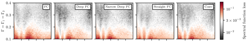
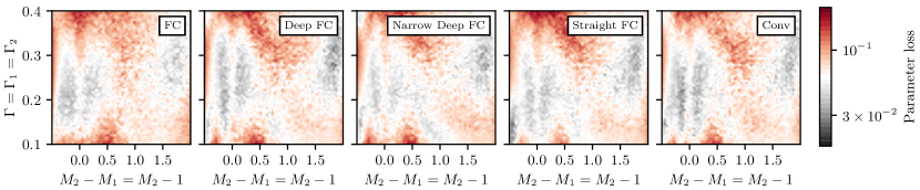
Figure 12: Comparison of network architectures - Contour plots of loss measures are shown for different net architectures. The upper three rows correspond to reconstructions of propagators with a noise width of $10^{-5}$, the lower ones with $10^{-3}$. The plots illustrate the loss measures in a hyperplane within the parameter space whose properties are described in Appendix C. The networks are trained with the parameter loss on the training set of volume Vol O. The contour plots show that the local minima are slightly different for small noise widths, whereas the global structures remain similar for all network architectures. These differences are caused by a slightly differing utilization of the limited number of hyperparameters. The differences between the network architectures become less visible for larger errors due to the growing severity of the inverse problem and a decreasing knowledge about the correct inverse transformations. Interestingly, the loss landscape of the convolutional neural network, which intrinsically operates on local structures, and of the fully connected networks are almost equal. The non-locality of the inverse integral transformation represents a possible reason for why the specific choice of the network structure is largely irrelevant. We conclude that the actual architecture is rather negligible in comparison to other attributes of the learning process, such as the selection of training data and the choice of the loss function.

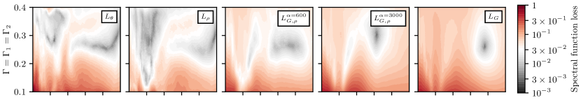
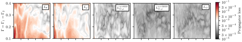
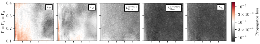
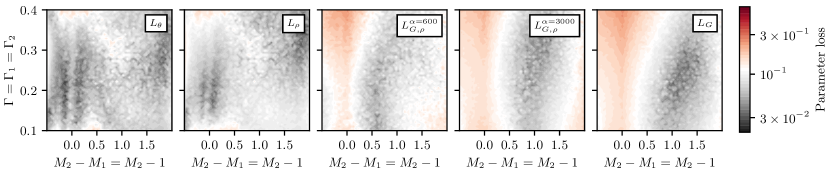
Figure 13: Comparison of loss functions - Contour plots of loss measures are illustrated in the same manner as in Figure 12, but with a comparison o different loss functions. The considered loss functions are introduced in Section III.2. The results are based on the Conv PaNet that is trained on volume Vol O. The optima in the loss function differ and, consequently, lead to different mean squared errors for the different measures. It is interesting that the network with the pure propagator loss function leads to a rather homogeneous propagator loss distribution. In contrast, the networks with the pure parameter and the pure spectral function loss do not result in homogeneous distributions for their corresponding loss function. The large set of nearly equal propagators for different parameters explains this observation. It confirms also once more the necessity of approaches that can be trained using loss functions with access to more information than just the reconstructed propagator.

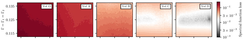
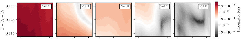
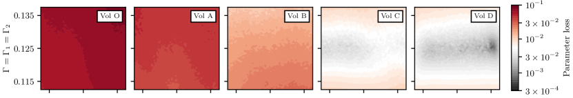
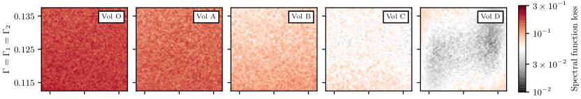
Figure 14: Analysis of prior information (parameter space of the training data) and of local differences in the severity of the inverse problem - The evolution of the landscape of different loss measures is shown for Conv PaNets that are trained on different parameter spaces. All contour plots are based on the same section of the parameter space, namely the range that is spanned by volume D. The upper three and lower rows correspond again to reconstructions of propagators with noise widths $10^{-5}$ and $10^{-3}$. The gradual reduction of the parameter space allows the analysis of different levels of complexity of the problem. A general improvement of performance can be observed besides a shift of the global optima. The more homogeneous loss landscape demonstrates that the problem of a different severity of the inverse problem is still present, but damped.

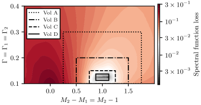
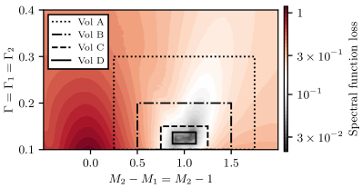
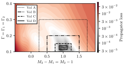
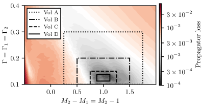
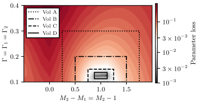
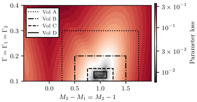
Figure 15: Performance outside of the training region - Performance of the Conv PaNet trained on the smallest volume Vol D for data that lies outside of the training region with a noise width of $10^{-5}$ (left column) and a noise width of $10^{-3}$ (right column). As expected, the prediction quality decreases with distance from the boundaries of Vol D. However, we emphasise that there is no immediate sharp transition at the boundary. Instead, we observe at first only a gradual decrease of the prediction quality, indicating that the network can generalise slightly beyond the trained region to varying degrees, depending on which parameters and error metrics are considered.

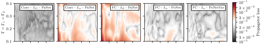
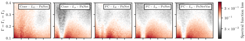
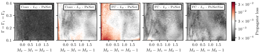
Figure 16: Comparison of the parameter net and the point net - Root-mean-squared-deviations are compared between the parameter net and the point net, trained on two Breit-Wigner like structures (PoNet) and trained on a variable number of Breit-Wigners (PoNetVar), with respect to different loss functions. The two upper rows correspond to results from input propagators with a noise width of $10^{-5}$ and the two lower ones with a noise width of $10^{-3}$. Problems concerning a varying severity of the inverse problem and concerning an information loss caused by the additive noise remain independent of the chosen basis for the representation of the spectral function.

Name		CenterModule		Number of parameters
FC		FC(6700) $\Rightarrow$ ReLU $\Rightarrow$ FC(12168) $\Rightarrow$ ReLU $\Rightarrow$ FC(1024)		$95\times 10^{6}$
Deep FC		FC(512) $\Rightarrow$ ReLU $\Rightarrow$ FC(1024) $\Rightarrow$ ReLU $\Rightarrow$ (FC(4056) $\Rightarrow$ ReLU$)^{3}$ $\Rightarrow$ (FC(2056) $\Rightarrow$ ReLU$)^{2}$		$50\times 10^{6}$
Narrow Deep FC		FC(512) $\Rightarrow$ ReLU $\Rightarrow$ (FC(1024) $\Rightarrow$ ReLU$)^{3}$ $\Rightarrow$ (FC(2056) $\Rightarrow$ ReLU$)^{5}$ $\Rightarrow$ (FC(1024) $\Rightarrow$ ReLU$)^{3}$ $\Rightarrow$ FC(512) $\Rightarrow$ ReLU $\Rightarrow$ FC(256)		$96\times 10^{6}$
Straight FC		(FC(4112) $\Rightarrow$ BatchNorm1D $\Rightarrow$ ReLU $\Rightarrow$ Dropout(0.2)$)^{7}$		$102\times 10^{6}$
Conv		Conv(64, 10) $\Rightarrow$ ReLU $\Rightarrow$ Conv(256, 10) $\Rightarrow$ ReLU $\Rightarrow$ (FC(4096) $\Rightarrow$ ReLU$)^{2}$ $\Rightarrow$ FC(1024)		$41\times 10^{6}$

Table 3: Details on the implemented network architectures. The argument of FC denotes the number of output neurons. The numbers in the argument of Conv correspond to the number of output channels and to the kernel size. The general setup is: Input(100) $\Rightarrow$ ReLU $\Rightarrow$ CenterModule $\Rightarrow$ ReLU $\Rightarrow$ FC(3/6/9/500) $\Rightarrow$ Output, where the CenterModule is given along with the associated name in the Table. The size of the output layer is determined by the use of a parameter net or a point net and the considered number of Breit-Wigners.

Figure	Network type	Architecture	Loss function	Training set	Test set	Noise width	Number of BWs
Figure 1	PaNet	FC	$L_{\theta}$	Vol O	Noise samples on same propagator	$10^{-3}$	1-3
Figure 3	PaNet	Various (a) / Conv (b)	$L_{\theta}$ (a) / Various (b)	Vol O	Vol O	$10^{-3}$ / $10^{-5}$	2
Figure 4	PaNet	Conv	$L_{\theta}$	Various	Noise samples on same propagator	$10^{-3}$	2
Figure 5	PaNet	Conv / Conv PP	$L_{\theta}$	Various	Vol D	Various	2
Figure 6	PaNet	Conv	$L_{\theta}$	Vol D	Various	Various	2
Figure 7	Various	FC	Various	Vol O	Vol O	Various	1-3
Figure 8	PaNet	Conv	$L_{\theta}$	Vol B	Noise samples on same propagator	Various	2
Figure 9	PaNet	FC / FC PP	$L_{\theta}$	Vol O	Vol O	Various	1-3
Figure 10	PaNet	FC	$L_{\theta}$	Vol O	Contour - Vol O	$10^{-3}$	2
Figure 11	PaNet	Conv	$L_{\theta}$	See Table 2	Specific sets	$10^{-3}$	1-3
Figure 12	PaNet	Various	$L_{\theta}$	Vol O	Contour - Vol O	$10^{-3}$ / $10^{-5}$	2
Figure 13	PaNet	Conv	Various	Vol O	Contour - Vol O	$10^{-3}$ / $10^{-5}$	2
Figure 14	PaNet	Conv	$L_{\theta}$	Various	Contour - Vol D	$10^{-3}$ / $10^{-5}$	2
Figure 15	PaNet	Conv	$L_{\theta}$	Vol D	Contour - Vol O	$10^{-3}$ / $10^{-5}$	2
Figure 16	Various	Conv / FC	Various	Vol O	Contour - Vol O	$10^{-3}$ / $10^{-5}$	2

Table 4: List of figures that contains details about the training of the different networks and about the dataset used for evaluation/validation.

References

- Guest et al. [2018] D. Guest, K. Cranmer, and D. Whiteson, Ann. Rev. Nucl. Part. Sci. 68, 161 (2018), arXiv:1806.11484 [hep-ex] .
- Radovic et al. [2018] A. Radovic, M. Williams, D. Rousseau, M. Kagan, D. Bonacorsi, A. Himmel, A. Aurisano, K. Terao, and T. Wongjirad, Nature 560, 41 (2018).
- LeCun et al. [2015] Y. LeCun, Y. Bengio, and G. Hinton, Nature 521, 436 (2015).
- Schmidhuber [2014] J. Schmidhuber, (2014), 10.1016/j.neunet.2014.09.003, arXiv:1404.7828 .
- Carrasquilla and Melko [2017] J. Carrasquilla and R. G. Melko, Nature Physics 13, 431 (2017).
- Shanahan et al. [2018] P. E. Shanahan, D. Trewartha, and W. Detmold, Phys. Rev. D 97, 094506 (2018).
- Carleo and Troyer [2017] G. Carleo and M. Troyer, Science 355, 602 (2017).
- Wetzel [2017] S. J. Wetzel, Phys. Rev. E 96, 022140 (2017).
- Wetzel and Scherzer [2017] S. J. Wetzel and M. Scherzer, Phys. Rev. B 96, 184410 (2017).
- Wang [2016] L. Wang, Phys. Rev. B 94, 195105 (2016).
- Hu et al. [2017] W. Hu, R. R. P. Singh, and R. T. Scalettar, Phys. Rev. E 95, 062122 (2017).
- Huang and Wang [2017] L. Huang and L. Wang, Phys. Rev. B 95, 035105 (2017).
- Liu et al. [2017] J. Liu, Y. Qi, Z. Y. Meng, and L. Fu, Phys. Rev. B 95, 041101 (2017).
- Karpie et al. [2019] J. Karpie, K. Orginos, A. Rothkopf, and S. Zafeiropoulos, JHEP 04, 057 (2019), arXiv:1901.05408 [hep-lat] .
- [15] J. M. Urban and J. M. Pawlowski, arXiv:1811.03533 .
- Bluecher et al. [2020] S. Bluecher, L. Kades, J. M. Pawlowski, N. Strodthoff, and J. M. Urban, (2020), arXiv:2003.01504 [hep-lat] .
- Jarrell and Gubernatis [1996] M. Jarrell and J. E. Gubernatis, Phys. Rept. 269, 133 (1996).
- Asakawa et al. [2001] M. Asakawa, T. Hatsuda, and Y. Nakahara, Prog. Part. Nucl. Phys. 46, 459 (2001), arXiv:hep-lat/0011040 [hep-lat] .
- Burnier and Rothkopf [2013] Y. Burnier and A. Rothkopf, Phys. Rev. Lett. 111, 182003 (2013), arXiv:1307.6106 [hep-lat] .
- Rothkopf [2019] A. Rothkopf, in 13th Conference on Quark Confinement and the Hadron Spectrum (Confinement XIII) Maynooth, Ireland, July 31-August 6, 2018 (2019) arXiv:1903.02293 [hep-ph] .
- [21] V. Shah and C. Hegde, arXiv:1802.08406 .
- [22] H. Li, J. Schwab, S. Antholzer, and M. Haltmeier, arXiv:1803.00092 .
- [23] R. Anirudh, J. J. Thiagarajan, B. Kailkhura, and T. Bremer, arXiv:1805.07281 .
- [24] L. Ardizzone, J. Kruse, S. Wirkert, D. Rahner, E. W. Pellegrini, R. S. Klessen, L. Maier-Hein, C. Rother, and U. Köthe, arXiv:1808.04730 [cs.LG] .
- [25] R. Fournier, L. Wang, O. V. Yazyev, and Q. Wu, arXiv:1810.00913 [physics.comp-ph] .
- Yoon et al. [2018] H. Yoon, J.-H. Sim, and M. J. Han, Physical Review B 98, 245101 (2018), arXiv:1806.03841 [cond-mat.str-el] .
- Cyrol et al. [2018] A. K. Cyrol, J. M. Pawlowski, A. Rothkopf, and N. Wink, SciPost Phys. 5, 065 (2018), arXiv:1804.00945 [hep-ph] .
- Oehme and Zimmermann [1980] R. Oehme and W. Zimmermann, Phys. Rev. D21, 1661 (1980).
- Oehme [1990] R. Oehme, Phys. Lett. B252, 641 (1990).
- Cuniberti et al. [2001] G. Cuniberti, E. De Micheli, and G. A. Viano, Commun. Math. Phys. 216, 59 (2001), arXiv:cond-mat/0109175 [cond-mat.str-el] .
- Burnier et al. [2011] Y. Burnier, M. Laine, and L. Mether, Eur. Phys. J. C71, 1619 (2011), arXiv:1101.5534 [hep-lat] .
- [32] C. Nogueira dos Santos, K. Wadhawan, and B. Zhou, 1707.02198 [cs.LG] .
- [33] L. Wu, F. Tian, Y. Xia, Y. Fan, T. Qin, J. Lai, and T.-Y. Liu, arXiv:1810.12081 [cs.LG] .
- Stan Development Team [2018] Stan Development Team, “Pystan: the python interface to stan, version 2.17.1.0,” http://mc-stan.org (2018).
- Carpenter et al. [2017] B. Carpenter, A. Gelman, M. D. Hoffman, D. Lee, B. Goodrich, M. Betancourt, M. Brubaker, J. Guo, P. Li, and A. Riddell, Journal of statistical software 76 (2017).