Using Convolutional Neural Networks to identify Gravitational Lenses in Astronomical images

Abstract

The Euclid telescope, due for launch in 2021, will perform an imaging and slitless spectroscopy survey over half the sky, to map baryon wiggles and weak lensing. During the survey Euclid is expected to resolve 100,000 strong gravitational lens systems. This is ideal to find rare lens configurations, provided they can be identified reliably and on a reasonable timescale. For this reason we have developed a Convolutional Neural Network (CNN) that can be used to identify images containing lensing systems. CNNs have already been used for image and digit classification as well as being used in astronomy for star-galaxy classification. Here our CNN is trained and tested on Euclid-like and KiDS-like simulations from the Euclid Strong Lensing Group, successfully classifying 77% of lenses, with an area under the ROC curve of up to 0.96. Our CNN also attempts to classify the lenses in COSMOS HST F814W-band images. After convolution to the Euclid resolution, we find we can recover most systems that are identifiable by eye. The Python code is available on Github.

1 Introduction

Gravitational lensing is caused by the mass of a foreground object, such as a galaxy or galaxy cluster, deflecting light from another distant source object, such as a galaxy or quasar. Strong gravitational lensing is rare with only a few systems expected from surveying thousands of objects (Blain, 1996). The first strong gravitational lens system, QSO 0957+561, was recognised as such in 1979 when the spectra of two objects were compared and confirmed to be from the same object (Walsh et al., 1979).

The Jodrell Bank-Very Large Array (VLA) Astrometric Survey (JVAS) (Patnaik et al., 1992; Browne et al., 1997) and the Cosmic Lens All-Sky Survey (CLASS) (Browne et al., 2003; Myers et al., 2003) have detected 22 radio loud lensed active galactic nuclei (Chae, 2003). Currently the Sloan Lens ACS Survey (SLACS) has provided the most strong lensed systems from a single survey with nearly 100 observed (Bolton et al., 2008). Other sources of strong lenses include the Kilo-Degree Survey (KiDS) (de Jong, Jelte T. A. et al., 2015) which uses the VLT Survey Telescope at the Paranal Observatory in Chile, the Dark Energy Survey (The Dark Energy Survey Collaboration, 2005), and the Subaru Hyper Suprime-Cam Survey (Miyazaki et al., 2012), expected to observed thousands of lenses (Collett, 2015). The BOSS Emission-Line Lens Survey (BELLS) have discovered at least 25 strong galaxy$-$galaxy gravitational lens systems with lens redshifts $0.4<z<0.7$, discovered spectroscopically by the presence of higher redshift emission lines within the Baryon Oscillation Spectroscopic Survey (BOSS) of luminous galaxies, and confirmed with high$-$resolution Hubble Space Telescope (HST) images (Brownstein et al., 2012).

Lensing systems are extremely useful cosmological tools. Lensed systems can be used to constrain the value of the Hubble constant, $H_{0}$, by measuring time delay (Refsdal, 1964; Kochanek & Schechter, 2004), which occurs because the light from multiple images has taken different paths to reach the observer, introducing a time delay. Cosmological distances are proportional to $c/H_{0}$, meaning $\Delta t=(1/H_{0})k$ where $k$ is related to the lens mass model. If a lens model can be found then we can predict $\Delta tH_{0}$ and infer $H_{0}$. Gravitational lensing is independent of the lensing object’s luminosity and depends only on the mass of the lens object and the geometry of the source and the lens relative to the observer. This makes lensing a unique tool for analysing mass distribution in the foreground lens (Treu & Koopmans, 2002). Using this dependence on mass alone, and combining mass models from mass$-$luminosity analysis, the baryonic and dark matter mass of the galaxy can be mapped to find dark matter substructure (Vegetti et al., 2012; Metcalf & Madau, 2001). Gravitational lensing conserves surface brightness (a consequence of Liouville’s Theorem) but not the angular size of the source object (Marchetti et al., 2017), causing a magnification of the source object’s flux, if the image of the source is enlarged. This enables the observation of fainter galaxies which would otherwise be missed, including galaxies at high redshifts (Claeskens et al., 2006; Jackson, 2011; Wyithe et al., 2011; Marchetti et al., 2017).

Future telescopes are expected to observe many more strongly lensed systems. The Euclid telescope (Laureijs et al., 2011) and the Large Synoptic Survey Telescope (LSST Science Collaboration et al., 2009), will bring the total number of systems above $10^{5}$ (Oguri & Marshall, 2010; Collett, 2015). Euclid will map three-quarters of the extragalactic sky with 0.2 arcsecond resolution to 24 AB magnitude (Amendola et al., 2018). Another project, the Square Kilometer Array (SKA) (Rawlings & Schilizzi, 2011), will take observations at a resolution of 2 milliarcseconds at 10 GHz, and 20 milliarcseconds at 1 GHz (Perley et al., 2009). The lensing surveys using SKA are expected to observe $\approx 10^{5}$ new radio$-$loud gravitational lenses (McKean et al., 2015; Serjeant, 2014).

There is currently a shift in the methodology for detecting strongly lensed systems in astronomical images as numbers of lens candidates becomes much larger. Traditionally most images were found by eye. 112 lens candidates, and at least 2 certain lenses, were found in a HST legacy programme, looking at the COSMOS field (Faure et al., 2008; Jackson, 2008). But not all searching by eye has been carried out by people working in strong gravitational lensing. The public have been tasked with finding new lens candidates through the Space Warps citizen science project (Marshall et al., 2016). Space Warps made use of volunteers analysing 430,000 images by eye to look for lensing features, via an online webpage using the Zooniverse platform. Tens of new lens candidates have been identified with the help of these volunteers, using large ground$-$based surveys, e.g. the Canada$-$France$-$Hawaii Telescope Legacy Survey (More et al., 2016). But with the growth of survey size there will be too many candidates to be examined by eye.

There have been several successful methods of computational searches for lenses. Arcfinder (Seidel, G. & Bartelmann, M., 2007), uses pixel-grouping methods to attempt to find cluster$-$scale lens systems. Ringfinder (Gavazzi et al., 2014), searches for blue residuals surrounding early$-$type galaxies using multi$-$band data, also there are several programs to find arc$-$like shapes (Lenzen, F. et al., 2004; More et al., 2012).

In recent years there has been a rise in machine$-$learning methods to detects lenses. 56 lens candidates were found in the KiDS dataset using a convolutional neural network (Petrillo et al., 2017). Machine learning methods rely on large datasets in order to train and learn, something which has become available in recent years. Once a machine has been trained, thousands of images can be classified in seconds. Speed is an important factor due to the expected $10^{9}$ images from Euclid (Collett, 2015). The use of citizen science could be used to create a dataset of images for machine learning techniques to train on, once trained, citizen science can then be applied again to examine the output images from the machine learning technique.

In section 2 we discuss neural networks and why we use them for this problem. In section 3 we discuss the simulated data we have used. In section 4 we discuss our convolutional neural network and how we trained it, and the results are discussed in section 5. The Python code is available at Github .

2 Why use Neural Networks

Computers are very effective at tasks with a limited set of rules, such as chess. However, humans are still often better at real world tasks which cannot easily be described by a set of rules, e.g. recognising objects. Artificial Neural Networks (NNs) are loosely inspired by how the brain works. They are made from simple computing elements with multiple inputs and one output analogous to a brain made up from neurons with dendrites and cell body receiving the inputs and axon outputting a signal. Like the brain, a NN can modify strengths of connections learnt from examples. Humans have evolved to be very fast and accurate at recognising objects, order of 100 ms (Thorpe et al., 1996). NNs, particularly Convolutional Neural Networks (CNNs) are the best available techniques in some tasks, e.g. translation, visual object recognition (LeCun et al., 2015). With current technology, a trained CNN can also perform these tasks faster than humans.

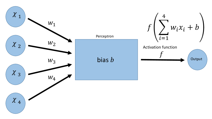
Figure 1: A perceptron with inputs $x_{1},x_{2},x_{3},x_{4}$, weights $w_{1},w_{2},w_{3},w_{4}$, bias $b$, and output calculated from the activation function $f$, together with the product of the weights and input and bias added.

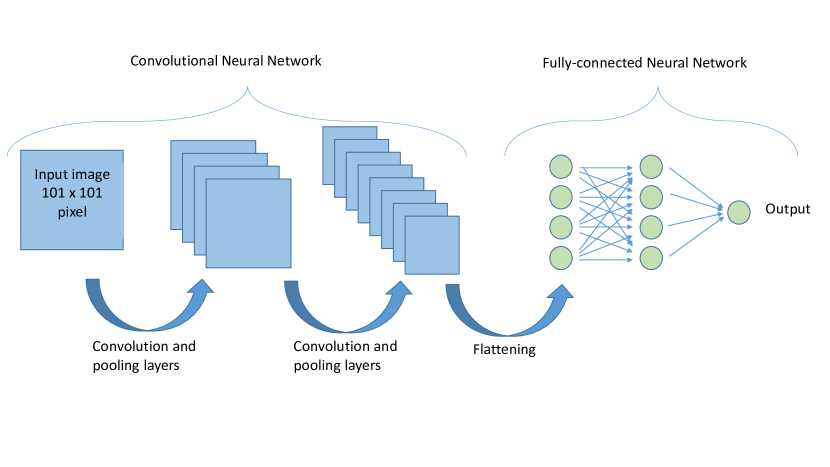
Figure 2: Diagram showing the architecture of the network and where the convolution layers are in respect to the fully-connected neural network. Not all layers shown.

Neural Networks are built from individual artificial neurons called perceptrons. A perceptron is designed to simulate the role of a biological neuron, but with the advantage that a mathematical function can be used for activation of the neuron (Aggarwal, 2014). A perceptron takes a number of inputs, applies a weight to each, sums these products, applies a bias, and then is used as input to an activation function, which then gives the perceptron’s output. Perceptrons can accept multiple inputs and apply different weights to each individual input. A perceptron with example inputs and outputs can be seen in Fig. 1. Individual scalar inputs are grouped together as a 1-d vector. If we let x be the 1-d vector of inputs, w be the 1-d vector of weights associated with this perceptron, $b$ be the bias, and $f$ be the activation function, then the output $z$ is calculated using:

$$z=f(\sum_{i=1}^{n}w_{i}x_{i}+b)$$ (1)

where $n$ is the number of inputs to the perceptron. In a NN, many perceptrons are grouped together to form a layer containing a few perceptrons to thousands. Layers use the outputs from previous layers as their inputs.

Neural Networks have to be trained before they can be used. For classification problems this involves passing many images of a known classification through the network in a process called supervised learning. The network classifies each image, and this output is combined with the true classification in a function called the loss function. A high value for the loss function means many images were incorrectly labelled by the network. The goal of training the network is to minimise the loss function over a number of passes of the training data. Each pass of the data is known as an epoch. After each epoch, the weights and biases are changed using Stochastic Gradient Descent (SGD), in order to minimise the loss function thereby increasing the rate of correct classifications from the network. The rate at which SGD changes the weights and biases is controlled by a variable called the learning rate. The is a linear parameter which controls by how much the weights and biases are changed. Using Adam (Kingma & Ba, 2014) instead of only SGD allows the learning rate to change as the network learns. Initially the learning rate starts off high, and decreases as the network becomes more accurate and the loss function value decreases. A small subset of images are used for data validation. After every epoch the validation images are classified and validation loss is recorded, calculated the same way as the training loss. The network is not trained on the validation data, so no changes are made to the weights and bias. Validation is done to prevent over-training the network. Training is stopped once the validation loss has reached a minimum. The validation loss will increase after this point as the network becomes over-trained, and this extra training is detrimental to classifying new datasets. After training has been completed, new images can be classified by passing the image through the network and obtaining a classification. Classifying an image makes no changes to the network parameters. Batch training means that the weights and biases are updated after seeing only a fraction of the training set. The batch number is typically small compared to the training number. Batch training is used to speed up training since the weights and biases are changed after each batch instead of at the end of each epoch.

CNNs are a subset of NNs which use convolutional layers in the network for feature recognition or classification. An example architecture of a CNN can be seen in Fig. 2. A convolutional layer involves a kernel being convolved with an input image in order to make a feature map. Often the convolution layer has several different kernels for the same image, meaning several different feature maps are given as output. The image kernel can either be pre-determined, or can be another parameter that the network trains and optimises. Different layers may have different image kernel sizes, as well as different sized image outputs. Between convolution layers, pooling layers are often inserted. A pooling layer is designed to greatly reduce the number of pixels in an input image to speed up training and reduce the number of parameters. Pooling is generally done one of two ways, max pooling or mean pooling. Both methods look at a small section of the image, say a $2\times 2$ section, and reduces this to one pixel value by either finding the maximum value in the $2\times 2$ square or by finding the mean. The output is then a reduced image with fewer pixels than the input. Pooling is done to reduce the number of variables whilst trying to keep as much spatial information as needed (Mallat, 2016). The convolution layers in a CNN are designed to process visual information hierarchically, with earlier layers finding more basic features, and later layers building on what layers before have found to create more complicated features within the image. This is how a network can go from seeing individual pixel values to finding complicated features, such as a face. After the convolutional layers, the network will have a layer to flatten the output from the final layer into a 1-d vector to be used as input for a layer composed of perceptrons. A layer in a network made from perceptrons that each use every output from the previous layer as input is known as a fully-connected or dense layer. All layers in NN apart from the input and output layer are known as hidden layers.

CNNs have been used to solve classification problems such as digit recognition with the MNIST database, a collection of 70,000 $32\times 32$ grey scale images of handwritten digits. The problem is to classify these as the digits 0 through 9. Using CNNs gives a solution with an error rate of 0.23% (Ciresan et al., 2013). CNNs have also been successful in object recognition in images. The CIFAR-10 database consists of 60,000 $32\times 32$ colour images in 10 classes, such as truck, bird and dog, with 6000 images per class. The error rate in this classification problem when using CNNs is lower than 4% . An astronomy classification problem where CNNs have been used is classifying images as a star or galaxy. Here the best network had an error rate of only 0.29% for galaxies (Kim2007; Dieleman2015).

3 Methods

The task of finding strong gravitational lenses in large datasets is a problem within Euclid. Feature recognition by eye will not be fast enough to cope with the amount of data received. The Strong Lensing group within the Euclid consortium set up the Euclid Strong Lensing challenge. This was a challenge aimed at developing machine learning techniques to classify images as to whether containing a lens or not. The simulated data was provided by the Bologna Lens Factory . The images are producing using GLAMER code (Metcalf & Petkova, 2014), which uses galaxies from the Millennium Simulation and real galaxies from KiDS (Kilo Degree Survey) as foreground lenses and background sources to produce the simulated images. More details of the lensing process can be found in (Metcalf et al., 2018). The simulated images are provided as $101\times 101$ pixel sized images, centred on the foreground galaxy, either containing a lensed source or not. In total 200,000 images were provided, 100,000 were Euclid VIS-like images, with $\approx$ 40,000 lenses and 100,000 were KiDS-like images, with $\approx$ 50,000 lenses. The Euclid-like space images are single band images, very broad band (r+i+z), whereas the KiDS-like images have four bands; $u,g,r,i$. The images have an image resolution of 0.2 arcsecond, meaning each is a $10\times 10$ arcsecond square image. Examples of the Euclid VIS-like images can be seen in Fig. 3, and an example of the 4 KiDS-like bands can be seen in Fig. 4. However our close scrutiny of the simulated images uncovered some unphysical examples. The COSMOS lenses , were used as a comparison to test the simulations against. Examples of the COSMOS lenses can be seen in the Appendix. The band used for the COSMOS images is the HST F814W wide band. F814W covers the longer wavelength half of the VIS throughput. Visual inspection of the VIS and smoothed COSMOS images shows qualitatively similar features. Therefore, we argue that the COSMOS data set is an appropriate and interesting test of our VIS-trained network.

By comparing histograms of the Einstein radius and lens magnitudes of both the simulated Euclid VIS-like images and the real COSMOS lens images, it was found that many of the simulations had unrealistically large Einstein rings, and that the Euclid VIS-like and KiDS-like simulations were fainter than the COSMOS lenses. Because of this, images with Einstein radii greater than 4 arcseconds, and lenses towards the faint end of the Euclid VIS-like and KiDS-like datasets have been removed in order to create a more representative subset. Histograms showing removal of some of the Euclid VIS-like images to make the dataset more COSMOS-like can be seen in Fig. 5. A similar histogram also shows that by removing the larger Einstein radii, the Euclid VIS-like images have an Einstein radius distribution similar to that of COSMOS. The same has been done for the KiDS-like dataset. In total we now have 4 datasets for training and 5 for testing which can be seen in Table. 1

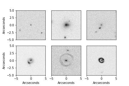
Figure 3: Samples from the 100,000 Euclid VIS instrument simulated images. The top row of images do not contain lenses, while the bottom row contains lenses.

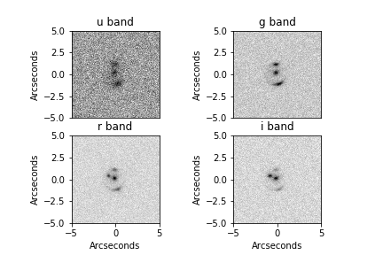
Figure 4: A sample from the 100,000 KiDS-like simulated images. The images are labelled above by their corresponding wavelength band. This example does contain lensing.

Figure 5: Histograms showing the AB magnitude across 3 datasets. Top: Original 100,000 Euclid VIS-like images, Middle: Subset of Euclid VIS-like images designed to have the same distribution as the COSMOS lenses, Bottom: The COSMOS lenses.

Table 1: Table describing the contents of each dataset.

Type	Description	Number of lenses
Euclid-VIS like simulations	100,000 single-band $1\times 101\times 101$ simulated images	39975
KiDS-like simulations	100,000 multi-band $4\times 101\times 101$ simulated images	49862
Euclid-VIS like simulations with COSMOS distribution	68,923 single-band $1\times 101\times 101$ simulated images	24029
KiDS-like simulations with COSMOS distribution	60,144 multi-band $4\times 101\times 101$ simulated images	29960
COSMOS lenses	65 single-band real lenses cropped to $101\times 101$ images	65

4 Training to find lenses

Four networks have been built, two designed to work with KiDS-like images with 4 filter bands as input, and two to work with Euclid VIS-like data with a single filter input. They have the same architecture, but have been trained on different data using datasets 1 through to 4 from Table. 1. The networks have been built and trained in Python 2.7 using the neural network library Keras . Keras runs on top of either Theano , TensorFlow or CNTK backends. We used Theano. The CNN architecture used here has been inspired by the work of (Petrillo et al., 2017). The network architectures can be seen in Table 2. Robust initialisation (HeNormal) is used to initialise the weights as this speeds up network convergence (He et al., 2015). The networks have 4 convolutional layers initially, with $2\times 2$ max-pooling incorporated twice after the first two convolutional layers. After the convolutional layers, the 2D feature maps that have been made in the final convolutional layer are flattened into a 1D vector to be used as input into the dense layer of fully connected neurons. The final layer is a classification layer, where the network gives each image a classification between 0 and 1. This number can been seen as a probability that the image is a lens. The CNN is trained on a set of 75% of the labelled images from the dataset, using a process of batch training with a batch size of 500. 5% of the dataset is used for data validation, to avoid over-training. Throughout our networks we used ReLU (Rectified Linear Units (Nair2010)) for the activation functions and binary cross-entropy was used as the loss function.

Table 2: Table shows the architecture of the 4 networks, Euclid VIS-like and KiDS-like. What each layers contains, as well as each layers initial weights and biases. The final sigmoid layer gives an output between 0 and 1. For the convolutional and max-pooling layers a stride length of 2 was used, meaning each pixel was only used once in pooling, padded with the same edge pixels where required.

Type of layer	Layer contains	Initial weights	Initial bias
Convolutional	8 ($15\times 15$) image kernels	HeNormal	Zeroes
Max-pooling	Pooled over each ($2\times 2$) square	-	-
Convolutional	8 ($15\times 15$) image kernels	HeNormal	Zeroes
Max-pooling	Pooled over each ($2\times 2$) square	-	-
Convolutional	16 ($5\times 5$) image kernels	HeNormal	Zeroes
Convolutional	16 ($5\times 5$) image kernels	HeNormal	Zeroes
Flatten	Convert image maps into 1-d vector	-	-
Dense	512 fully-connected neurons	HeNormal	Zeroes
Dense	1 sigmoid output neuron	HeNormal	Zeroes

5 Results and Discussion

An image is judged to contain a lens if the classification from the network is above or equal to $0.5$, conversely if the classification is below $0.5$ the image is judged to not contain a lens. This value can be increased to give a more accurate classification, causing the number of false positives to decrease. However it also means that more lenses are misclassified. 20% of each dataset is passed through the appropriate network to be classified; this is the test set. The scores for each network can be seen in Table. 3. By looking at the percentage of images classified correctly, and the percentage of lenses and non-lenses classified correctly, the KiDS-like networks are more successful than the Euclid VIS-like networks. This is not surprising since the KiDS-like images have 4 image bands compared to the single band of the Euclid VIS-like images. This would imply that colour information from the multiple bands of the KiDS-like images has been helpful in classifying the lenses correctly, as one would expect as it helps greatly when classifying by eye. A test of this (which we will conduct in future work) would be to compare single-band KIDS-like images with multi-band KIDS-like images. In both the COSMOS-like datasets, the percentage of lenses correctly identified is less than the original datasets. This is probably because the images with the largest rings (> 4 arcseconds Einstein radius) have been removed to make the dataset. These images are easy to identify as lenses and so removing them decreases the success rate for lenses. However non-lens classification success has increased with the same number of non-lens images involved. Although both the datasets have a similar overall success rate, the network trained on the Euclid VIS-like dataset performed significantly worse at recognising the images containing lenses. The difference in overall performance is most clear by looking at the Receiver Operating Characteristic (ROC) curves for the datasets together in Fig. 6. A true positive is when a true image, one with a lens, is classified as such, while a false positive is when a false image, one without a lens, is classified as having a lens. The area under the ROC curve determines the results, 1 being the score for all classifications correct, 0 the score for all classifications incorrect, and 0.5 being the result of random selection. True negatives and false negatives are defined similarly. Fig. 6 confirms that the KiDS-like dataset performed best, although the network only improved slightly using a subset of the images, unlike the Euclid dataset which improved significantly by removing images from the dataset.

As well as using simulated data, we tested on 65 real images from COSMOS. These are single-band images made from larger image cutouts and modified to have the same PSF as the Euclid images by convolving with a suitable kernel. The full width at half maximum (FWHM) of Euclid squared is equal to the FWHM of COSMOS squared plus the FWHM of the kernel squared;

$$FWHM(Euclid)^{2}=FWHM(COSMOS)^{2}+FWHM(kernel)^{2}$$

After convolution to match the Euclid PSF, the COSMOS images also had their pixels resampled to match the Euclid pixel scale. Images of the COSMOS lenses before and after applying the convolution can be seen in the Appendix. The resulting images were also $101\times 101$ pixels. Having only 65 available images meant that training on these images was not a possibility, but testing them with the trained Euclid-like networks was. The results can be seen in Table. 4. The scores for both networks were very low, and can be expected after training on a different type of image. Every COSMOS lens that has been classified incorrectly is a false negative. All of the images from the COSMOS survey can be seen in the Appendix. Nevertheless, our network recovers 16/31 of the lenses identifiable by eye at the Euclid resolution (see Appendix), and 8/34 of the lenses that cannot be identified by eye. Although our network at Euclid resolution only recovers $20\%$ of the lenses known to exist at HST resolution, this is in itself quite interesting: it implies that the detectability of lensing is a very strong function of angular resolution. Roughly doubling the angular resolution (from Euclid to HST resolution) results in roughly a five-fold increase in the numbers of detectable lensing systems.

Even though the KiDS-like subset showed a great deal of success, there are still things to be wary of: all the images used in this work in training and testing are simulated images, but real images may not be classified as accurately, which can be seen by looking at the results from the COSMOS images. The percentage of images containing a lens is much higher in these simulated cases than for real data.

Once implemented with real data, the number of lenses observed will increase. This in turn will increase the number of rare lens systems found, such as double-source plane lens systems (Collett & Auger, 2014). These rare systems can be used to constrain the dark-energy equation of state parameter $w$ (Gavazzi et al., 2008). Lens models can be made from the systems observed, and when coupled with visible images can infer dark matter substructure within the lensing galaxy.

Future work will include training and testing the networks on updated simulations incorporating cluster lenses and Eulcid’s grism data. The problems from these first simulations have been noted so that the next training set will not include large Einstein rings (> 4 arcsecond) and will add more complex images to classify, such as face on spiral galaxies. A further complication to be modelled is the diversity of non-lensed interloper populations, such as polar ring galaxies, or galaxies with tidal tails. The most effective approach here may be to degrade HST images to an appropriate Euclid-like resolution. However, the network presented here will be an excellent starting point for training quickly on such a more comprehensive training set, because CNNs can be efficiently adapted to new but similar application domains (Domínguez Sánchez et al., 2018). The networks will also be trained and tested on different simulations from Collett (2015).

Table 3: This table shows the percentage of images classified correctly, for lenses, non-lenses and total correct.

Images	Lenses Correct (%)	Non-Lenses Correct (%)	Total Correct (%)
Euclid VIS-like simulations	60.32	93.26	80.13
KiDS-like simulations	88.17	86.82	87.49
Euclid VIS-like simulations with COSMOS distribution	56.14	98.86	93.33
KiDS-like simulations with COSMOS distribution	76.83	97.46	93.62

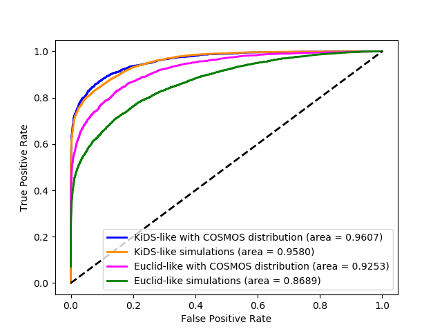
Figure 6: Receiver operating characteristic curves for Euclid network (top) and KiDS network (bottom) with the area under the curve shown. The black dashed line indicates the curve for random choice.

Table 4: Table containing the classification results of the COSMOS lenses on two differently trained networks. Note all 65 images were lenses.

Trained Dataset	Lenses Correct
Euclid VIS-like simulations	18 (27.69%)
Euclid VIS-like simulations with COSMOS distribution	15 (20.00%)

6 Conclusions

A well designed CNN can be used with future observations from Euclid and other similar surveys as they are demonstrably successful on simulated data. Making more realistic simulations, more accurate distributions of Einstein radii and faint lens galaxies, will give a more accurate account of how CNNs will perform with real data. Machine learning techniques will provide a subset of ostensibly reliable lens systems where verification by visual inspection can be achieved in a realistic time$-$scale which can then be used to refine the CNN.

Appendix A COSMOS Lenses

The following figures show the 65 lenses from COSMOS that our CNNs were tested with. Each lens has the ID number below. Images with an asterisk after the ID number were the ones that were correctly identified as a lens. Each image has the usual North up, East left configuration, and are 10$\times$10 arcseconds. Images in the left column are from the COSMOS survey, in the right are the same images after being convolved with a kernel to give the image the same PSF as Euclid. The images have been grayscale altered to best show the lens.

0009+2455                            0012+2015

0013+2249                            0018+3845*

0028+1919                            0029+4018

0038+4133*                            0047+2931

0047+5023                            0049+5128*

0050+0357*                            0050+4901

0055+3821*                            0056+1226*

0056+2106                            0104+2046

0104+2501*                            0105+4531*

0107+0533                            0108+5606

0120+4551                            0124+5121*

0148+2325                            0208+1422*

0211+1139*                            0216+2955

0220+2335*                            0221+3440

0227+0451*                            0236+4807

0248+1422                            5748+5524

5750+5619                            5752+2057

5754+5952                            5758+1525*

5805+0413*                            5806+5809

5821+4437                            5829+3734

5831+4332*                            5841+4646

5851+1813                            5856+4755

5857+5949                            5906+4524

5914+1219*                            5919+3853

5921+0638*                            5924+0852

5925+3039                            5929+1352

5929+4553*                            5931+0229

5932+1018*                            5936+3621

5939+3044                            5940+3253

5940+5012                            5941+3628*

5942+2829*                            5943+2816

5947+4752*                            5951+1236

5959+0348

References

- Aggarwal (2014) Aggarwal C. C., 2014, Data classification: algorithms and applications.. Chapman & Hall, CRC Press
- Amendola et al. (2018) Amendola L., et al., 2018, Living Reviews in Relativity, 21, 2
- Blain (1996) Blain A., 1996, mnras, 283, 1340
- Bolton et al. (2008) Bolton A. S., Burles S., Koopmans L. V. E., Treu T., Gavazzi R., Moustakas L. A., Wayth R., Schlegel D. J., 2008, ApJ, 682, 964
- Browne et al. (1997) Browne I., Jackson N., Augusto P., Henstock D., Marlow D., Nair S., Wilkinson P., 1997
- Browne et al. (2003) Browne I. W. A., et al., 2003, Monthly Notices of the Royal Astronomical Society, 341, 13
- Brownstein et al. (2012) Brownstein J. R., et al., 2012, ApJ, 744, 41
- Chae (2003) Chae K.-H., 2003, Monthly Notices of the Royal Astronomical Society, 346, 746
- Ciresan et al. (2013) Ciresan D. C., Giusti A., Gambardella L. M., Schmidhuber J., 2013, in MICCAI. pp 411–418
- Claeskens et al. (2006) Claeskens J.-F., Sluse D., Riaud P., Surdej J., 2006, A&A, 451, 865
- Collett (2015) Collett T. E., 2015, The Astrophysical Journal, 811, 20
- Collett & Auger (2014) Collett T. E., Auger M. W., 2014, Monthly Notices of the Royal Astronomical Society, 443, 969
- Domínguez Sánchez et al. (2018) Domínguez Sánchez H., et al., 2018, preprint, (arXiv:1807.00807)
- Faure et al. (2008) Faure C., et al., 2008, The Astrophysical Journal Supplement Series, 178, 382
- Gavazzi et al. (2008) Gavazzi R., Treu T., Koopmans L. V. E., Bolton A. S., Moustakas L. A., Burles S., Marshall P. J., 2008, ApJ, 677, 1046
- Gavazzi et al. (2014) Gavazzi R., Marshall P. J., Treu T., Sonnenfeld A., 2014, The Astrophysical Journal, 785, 144
- He et al. (2015) He K., Zhang X., Ren S., Sun J., 2015, in The IEEE International Conference on Computer Vision (ICCV).
- Jackson (2008) Jackson N., 2008, MNRAS, 389, 1311
- Jackson (2011) Jackson N., 2011, ApJ, 739, L28
- Kim (2007) Kim J., 2007, Monthly Notices of the Royal Astronomical Society, 375, 625
- Kingma & Ba (2014) Kingma D. P., Ba J., 2014, CoRR, abs/1412.6980
- Kochanek & Schechter (2004) Kochanek C. S., Schechter P. L., 2004, Measuring and Modeling the Universe, p. 117
- LSST Science Collaboration et al. (2009) LSST Science Collaboration et al., 2009, preprint, (arXiv:0912.0201)
- Laureijs et al. (2011) Laureijs R., et al., 2011, preprint, (arXiv:1110.3193)
- LeCun et al. (2015) LeCun Y., Bengio Y., Hinton G., 2015, Nature, 521, 436
- Lenzen, F. et al. (2004) Lenzen, F. Schindler, S. Scherzer, O. 2004, A&A, 416, 391
- Mallat (2016) Mallat S., 2016, Philosophical Transactions of the Royal Society of London Series A, 374, 20150203
- Marchetti et al. (2017) Marchetti L., Serjeant S., Vaccari M., 2017, MNRAS, 470, 5007
- Marshall et al. (2016) Marshall P. J., et al., 2016, MNRAS, 455, 1171
- McKean et al. (2015) McKean J., et al., 2015, Advancing Astrophysics with the Square Kilometre Array (AASKA14), p. 84
- Metcalf & Madau (2001) Metcalf R. B., Madau P., 2001, ApJ, 563, 9
- Metcalf & Petkova (2014) Metcalf R. B., Petkova M., 2014, Monthly Notices of the Royal Astronomical Society, 445, 1942
- Metcalf et al. (2018) Metcalf R. B., et al., 2018, preprint, (arXiv:1802.03609)
- Miyazaki et al. (2012) Miyazaki S., et al., 2012, Hyper Suprime-Cam, doi:10.1117/12.926844, https://doi.org/10.1117/12.926844
- More et al. (2012) More A., Cabanac R., More S., Alard C., Limousin M., Kneib J.-P., Gavazzi R., Motta V., 2012, The Astrophysical Journal, 749, 38
- More et al. (2016) More A., et al., 2016, Monthly Notices of the Royal Astronomical Society, 455, 1191
- Myers et al. (2003) Myers S. T., et al., 2003, MNRAS, 341, 1
- Oguri & Marshall (2010) Oguri M., Marshall P. J., 2010, MNRAS, 405, 2579
- Patnaik et al. (1992) Patnaik A. R., Browne I. W. A., Walsh D., Chaffee F. H., Foltz C. B., 1992, MNRAS, 259, 1P
- Perley et al. (2009) Perley R., et al., 2009, IEEE Proceedings, 97, 1448
- Petrillo et al. (2017) Petrillo C. E., et al., 2017, MNRAS, 472, 1129
- Rawlings & Schilizzi (2011) Rawlings S., Schilizzi R., 2011, preprint, (arXiv:1105.5953)
- Refsdal (1964) Refsdal S., 1964, MNRAS, 128, 295
- Seidel, G. & Bartelmann, M. (2007) Seidel, G. Bartelmann, M. 2007, A&A, 472, 341
- Serjeant (2014) Serjeant S., 2014, ApJ, 793, L10
- The Dark Energy Survey Collaboration (2005) The Dark Energy Survey Collaboration 2005, ArXiv Astrophysics e-prints,
- Thorpe et al. (1996) Thorpe S., Fize D., Marlot C., 1996, Nature, 381, 520
- Treu & Koopmans (2002) Treu T., Koopmans L. V. E., 2002, Monthly Notices of the Royal Astronomical Society, 337, L6
- Vegetti et al. (2012) Vegetti S., Lagattuta D. J., McKean J. P., Auger M. W., Fassnacht C. D., Koopmans L. V. E., 2012, Nature, 481, 341
- Walsh et al. (1979) Walsh D., Carswell R. F., Weymann R. J., 1979, Nature, 279, 381
- Wyithe et al. (2011) Wyithe J. S. B., Yan H., Windhorst R. A., Mao S., 2011, Nature, 469, 181
- de Jong, Jelte T. A. et al. (2015) de Jong, Jelte T. A. et al., 2015, A&A, 582, A62