How to Find a Planet from Transit Variations

Abstract

Here we describe a story behind the discovery of Kepler-46, which was the first exoplanetary system detected and characterized from a method known as the transit timing variations (TTVs). The TTV method relies on the gravitational interaction between planets orbiting the same star. If transits of at least one of the planets are detected, precise measurements of its transit times can be used, at least in principle, to detect and characterize other non-transiting planets in the system. Kepler-46 was the first case for which this method was shown to work in practice. Other detections and characterizations followed (e.g., Kepler-88). The TTV method plays an important role in addressing the incompleteness of planetary systems detected from transits.

My background is in dynamical astronomy. This is a branch of astronomy that is concerned with the motion of planets, stars and galaxies. Somehow, something clicked while I was attending lectures about dynamical astronomy as an undergraduate at the Charles University in Prague. I remember really enjoying the mathematical methods that we were asked to master. In other astronomy courses, we learned key equations with many variables. Their derivation was standard, they expressed interesting relations, but they left me unsatisfied. I think I really wanted to use advanced mathematics that we have just learned in other courses, and operating ratios of astrophysical variables was not exactly that.

Now, the field of dynamical astronomy has a very long history, going back to Kepler, Newton, Laplace, Le Verrier, Poincaré and Brouwer, to mention just a few names. The mathematical methods these guys developed are fantastic. They include Hamiltonians, perturbation theories, resonances, chaos. Finally, I had the satisfactory feeling of actually using mathematics to understand fragments of the physical world. My colleagues got discouraged for exactly the same reason, and moved to other research, as far from the Hamiltonians as they could. The subject of my Master thesis was an obscure topic of orbital dynamics of asteroids near resonances with Jupiter, the scope of my doctorate was only inches broader. Still, these early days gave a good dose of useful scientific background.

The exoplanet discoveries in the past two decades were one of two revolutions that I witnessed at close range (the other one being the Velvet Revolution of 1989). New exoplanets are announced every month. The smallest, the one with the shortest orbital period, the most distant one, a system of three, four or even more planets. I remember watching these inspiring discoveries and wondering about how to make sense of the diversity that was emerging from observations. I still wonder about that now.

The lack of data bothered me quite a bit in the early days, when exoplanet science was essentially an observational endeavor. Sure, one could start developing theories of this and that, but where is the assurance, given the paucity of constraints, that they could be correct. To this day, I still think that the detection and characterization of exoplanets is the top priority. That could be a dead end for a theorist like me, but back in 2007, after reading a few papers published a couple of years earlier, I got intrigued by the method known as the transit timing variations or TTVs for short. The method is straightforward. If there is just one transiting planet and no complications, the planetary transits must be occurring on a linear ephemeris. That is exactly on a linear ephemeris, as defined by the planet’s orbital period. Once you add planets, however, they start pulling on each other, and their orbits are strictly Keplerian no more; compared to a linear ephemeris, some transits occur earlier and some later. That is what the TTVs stand for.

The promise of the TTV method was that if there is, say, transiting Neptune closer in and an Earth-size planet farther out, then the inner planet’s TTVs should reveal the existence of the outer planet. No other observations needed. Awesome, isn’t it!? That was the theme that the first paper, by Holman & Murray (2005), highlighted. The second paper, by Agol et al. (2005), was broader in scope. It discussed TTVs for all sorts of planetary configurations and gave an approximate scaling of the TTV amplitude for each.

So far so good, I recall thinking, but how about the heart of the matter, which is the inverse problem. The inverse problem arises when someone attempts to figure out the planetary parameters, such as the mass and orbit, from TTVs. Does the inverse problem have a unique solution? What if the companion planet is not transiting?

My goal in 2007/2008 was somewhat naive, I thought it could be possible to fully resolve the inverse TTV problem by employing computer algebra. For that I considered a case where there are two planets orbiting the same star, and the orbital period ratio of the two planets is not in a ratio of small integers (i.e., the non-resonant orbits in a scientific jargon). There is a well known mathematical method, known as the Lie-Hori perturbation theory, that can be applied to this case. Furthermore, in practice, the observational coverage of any given system is relatively short, years to tens of years max. So, one only needs to consider the short-period variations, and ignore everything else. This turns out to be relatively easy. The interaction potential is expanded in the Fourier series and the short-period variations of orbital elements emerge in the Lie-Hori theory as derivatives of the generating function, which is closely related to the original Fourier expansion. The variations are then plugged into an expression for TTVs, and voila, the TTVs are given as the Fourier series as well.

I reasoned that an observer can take the TTV data and perform the Fourier analysis, thus identifying frequencies, amplitudes, and phases of whatever terms the measurements contain. The short-period frequencies must be $k_{1}n_{1}+k_{2}n_{2}$, where $k_{1}$ and $k_{2}$ are small integers, and $n_{1}$ and $n_{2}$ the orbital frequencies of the two planets (here, 1 is the inner transiting planet and 2 is the outer one). The periods of these terms are comparable to the orbital periods and that’s why they are called the short-period TTVs. There is a slight complication as some identified frequencies can be aliases of $k_{1}n_{1}+k_{2}n_{2}$. Still, given a set of frequencies, it should be possible to figure out which ones are real and which ones are aliases, eventually giving us $n_{2}$ (frequency $n_{1}$ is known from transits).

It then remains to match the observed amplitudes and phases to their theoretical expressions and we have a set of equations to compute unknowns, including masses of the two planets and their six orbital elements. That is, in general, 14 unknowns. Not all unknowns, however, can be determined from TTVs. For example, the unknown orbit orientation with respect to the sky plane causes a degeneracy in the nodal longitudes. The TTVs can be used to determine the difference, $\Omega_{1}-\Omega_{2}$, but not the individual values. Also, the true longitude of the transiting planet is known from the transit observations. So there are really only 12 unknowns. So, if the goal is to determine every parameter, at least 6 frequency terms need to be measured in the TTV signal. This gives six equations for phases and six for amplitudes, i.e., 12 equations and 12 unknowns, as it should be.

Well, what seems simple in theory is not easy in practice, mainly because the equations are ugly and difficult to deal with. Rather than struggling with the analytic solution, I realized that it would more practical to do things numerically, and my goals shifted. Still, while my original plan somewhat predictably failed, I learned many things from this exercise. It occurred to me, for example, that the analytic method can be used to greatly speed up the whole process of inversion.

To appreciate that, let’s take a modern viewpoint on this issue and consider a purely numerical method. Say that an efficient N-body integrator is instructed how to compute the transit times for any given planetary system. The code is interfaced with some smart algorithm that knows how to maximize the likelihood of the fit. All that is OK, but the basic difficulty is that the algorithm must search in parameter space of 12 dimensions, which is a lot of dimensions. The program may take too long to execute or it may not converge at all if the likelihood landscape is too complex. It all depends on how much CPU time it takes to compute transits for one planetary configuration.

I developed a fully numerical code and tested it on mock planetary systems back in 2008. Things were annoyingly slow. So, I explored every avenue to speed things up. For example, do we gain anything if the N-body code is replaced by the Fourier routines that calculate TTVs analytically? If so, they can perhaps be used to determine an approximate solution, and the N-body integrator can take over after that.

It turns out that the 12 variables can be split in four groups. The first and the most difficult to deal with are the semimajor axes of the two planets. The coefficients of the Fourier series depend on them in non-trivial ways. Fortunately, they depend only on the ratio of the semimajor axis, $\alpha=a_{1}/a_{2}$, and not on $a_{1}$ and $a_{2}$ individually. So, it is possible to precompute all coefficients on a grid in $\alpha$ and devise a fast algorithm that interpolates from the grid to any value of $\alpha$. The likelihood of the fit is a very sensitive function of $\alpha$, so the grid must be sufficiently dense for things to work. [In fact, it is even better to work with the orbital periods (rather than the semimajor axes), because of uncertainties in stellar mass.]

The second group is the orbital eccentricities and inclinations. The coefficient dependence on them is simple: they appear in all powers permitted by symmetries. It turns out to be possible to develop recursive routines to compute the higher powers from the lower ones such that the number of arithmetical operations is minimized.

The third group are the orbital angles, three for each planet. A really efficient way to evaluate the Fourier series for any combination of angles is to make use of complex algebra and symmetries. The algorithm computes a few leading terms and combines them to get the remaining ones almost for free. Therefore, in essence, because the evaluation of the Fourier series for angles is so inexpensive, one can set aside the angle dimensions. This effectively reduces the dimension of the problem.

The last group is the masses of the two planets. The TTVs of the inner transiting planet are nearly independent of its own mass and depend linearly on the mass of the outer planet. So, there is no hope, in absence of other information, to determine the mass of the transiting planet from its short-period TTVs. On the other hand, since the dependence on the perturbing planet’s mass is linear, the algorithm can first compute TTVs for some indeterminate mass, and subsequently adjust $m_{2}$ to optimize the fit. Again, this is cheap.

These are some of the main features of the code I developed in 2008. In the final version, the algorithm based on the perturbation theory was many orders of magnitude faster than the N-body approach. It counts, you know, if the calculation can be done in minutes instead of many weeks.

The radial velocity observations of warm and cold Jupiters indicate that these planets often have large orbital eccentricities. Their orbits were presumably excited by dynamical instabilities and gravitational scattering. So, to make my analytic algorithm applicable to these cases, I pushed the perturbation theory to very high powers of eccentricity, first to 5, then to 15, and finally to 25. This means that all terms in eccentricities up to power 25 were included in the final code. In retrospect, this was unnecessary because the Kepler observations showed that the TTV planets regularly have almost circular orbits.

There were various hiccups while the code was being developed and tested. Some were more serious than others. In most cases, I was able to link these problematic cases to systems that were too compact, too close to resonances or something else, but sometimes a perfectly normal system was giving me a trouble. After weeks and weeks of struggle, with the problem seemingly going away and then coming back when I least expected it, I started to suspect that the Fourier expansion of the potential is at fault. I have adapted this part of the code from another program that was given to me by my former teacher and advisor, Miloš Šidlichovský, who developed and used it for other projects.

It took some courage to start suspecting that something funky is going on in that part of the code, because Miloš is a very careful man. I would rather expect to find a bug in my code. Tracking the issue down, however, I found that some coefficients of the expansion are exactly two times smaller than they should be, and applied an empirical patch in the code that compensated for that. With that, things fell in place. I later visited Miloš just before his retirement from the Czech Academy of Sciences. When I described the problem to him, he said, of course, you are using the program to do things that it was not meant to do, and then proceeded to figure out what the real problem was.

After 2008, I was ready to use my new algorithms to do things, but did not have any good data to try them on. Before Kepler, TTVs were measured for hot Jupiters and alike, which do not have planetary companions too often. Also, companions would need to be fairly close or near resonant period ratios for the TTV method to work. In addition, the ground-based transit observations produced TTVs with rather large measurement errors and sparse transit coverage. That was not good enough for solving the inverse problem. I knew that well because I was experimenting on mock systems, where I would inject realistic measurement errors in the TTV data and vary the number of observed transits. It turns out that even for an excellent signal-to-noise (Kepler-46 has $S/N\sim 50$, where $S/N$ is defined here as the ratio of the observed TTV amplitude to the timing measurement uncertainty), one still needs at least about 15 transits, continuous or not, for the inverse problem to have a unique solution.

The Kepler mission, of course, changed that, but not being part of the Kepler team did not help. Thus, I became somewhat disheartened while watching the discoveries of Kepler-9b,c, which was the first planetary system characterized from TTVs (Holman et al. 2010), Kepler-19b, which was the first case that showed clear TTV evidence for an unseen planet (Ballard et al. 2011), and others. It looked as if the train departed leaving me behind. In the meanwhile, I improved the validity of the codes for strongly inclined systems and eccentric transiting planets, performed a tentative analysis of COROT-1b, TrES-1b and HD 189733b, and waited for something.

That something happened in November 2011 when I was on a sabbatical leave at the Nice observatory, in southern France. I received an unexpected email from David Kipping, then Carl Sagan Fellow at the Harvard-Smithsonian Center for Astrophysics. David invited me to be a member of a small team of researchers known as the Hunt for Exomoons with Kepler (HEK; Kipping et al. 2012). Other then David and me, the HEK staff included Gáspár Bakos from Princeton University and Allan Schmitt from PlanetHunters.org. Small teams suit me well and knowing David from before I gladly accepted. My role in the team was to use Kepler TTVs, which David extracted with formidable speed and accuracy from the MAST catalog, to characterize planets.

The following part of the story, which eventually led to the detection and characterization of Kepler-46 and the publication of this work in the Science magazine, is best told by an email exchange among the HEK members. Below I reproduce excerpts from some of these emails along with short commentaries. In the following text, the dates of the emails are given in the US convention (MM/DD/YYYY).

From David K’s email to the HEK team (11/27/2011):

HCV-439 is the most interesting system. The system exhibits TTVs of $\sim$1 hour amplitude whereas none of the other systems have ‘clean’ TTVs like this.

I attach here the TTVs of the top four candidates. HCV-439 is the only one with a really convincing signal.

The highest priority is HCV-439. Could you please run your code on these TTVs and see what planetary solutions are valid (if any)? Let me know if you need any other system parameters. Note that the system is known to only have one transiting planet thus far.

Note that HCV-439, mentioned in the above email, was our HEK nickname for KOI-872, which later became known as Kepler-46. We used a nickname to avoid potential information leaks.

From David N’s email on 12/1/2011:

I made some initial attempts to fit the TTV signal for 439. So far I only tried co-planar systems. There are many solutions that provide a good match to the data.

The plot illustrates the importance of getting additional transits. With only one additional transit, it will be clearly possible to distinguish between the three solutions shown here. I expect that the unique solution will be found when we will have $\sim$10 transits.

This saw-tooth pattern looks to me like a short-period planetary signal which is ideal for my method (resonant oscillations would have longer period).

One solution gives normalized chi2$<$0.1 and stands out as exceptionally good. This could be the right one. It corresponds to a planet half the Jupiter mass at $a=0.29$ AU and $e=0.1$. It may or may not be the right one.

It turns out that the best solution mentioned above is essentially the right one. This is amazing, because we only had 6 (!) transits of KOI-872b in late 2011, when this email was written (Figure 1).

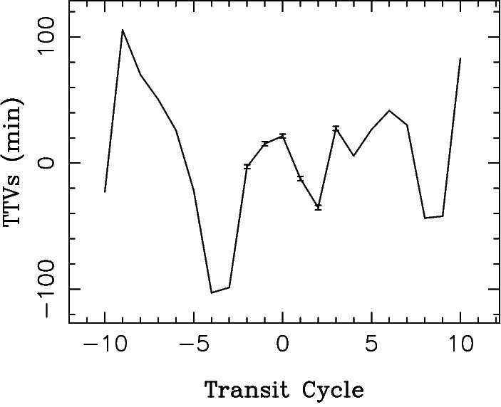
Figure 1: From our early attempts to fit TTVs of KOI-872b.

From David K’s email on 12/1/2011:

Excellent stuff. It is frustrating that we only have 6 transits. In January we should acquire additional $\sim$10 transits so we will then have more than enough.

The TDVs are significant so I suspect there is important information in there and I look forward to seeing what happens when you fit the TTV and TDV simultaneously.

David K was rightly pointing out the importance of transit duration variations (TDVs). The lack of TDVs of KOI-872 was later used to reject the second best solution and obtain a unique fit.

From David N’s email on 12/9/2011:

With 6 transits it is impossible to do anything reasonable with non-coplanar systems, so I focused on coplanar planetary fits.

For the moment I looked at the semimajor axis range of the putative planet between 0.17 to 1 AU. There are 30 solutions where analytic fits to observed TTVs showed normalized chi2$<$1. This cut is arbitrary.

I would like to briefly highlight the first solution in the list below, corresponding to a planet about half the Jupiter mass with 80 day period and 0.1 eccentricity. Attached plot shows the TTVs and TDVs for this system. TTVs look pretty good.

The ‘first’ solution mentioned in my Dec. 9 email was published as the second-best solution (s2) in our Science article. This solution can be rejected with more TTV data and TDVs.

From David K’s email on 12/9/2011.

This is all really cool. So either we have a moon or a 2nd planet then. I wonder if there is any way to constrain the mass of the transiting planet, even a broad limit such as Mp$<$10 Mj (i.e. a real planet rather than a false positive)? So what I’m really asking is can we confirm this candidate?

Again, this is spot on. We could not obtain any limits on the mass of the transiting candidate from the TTV data available to us in 2011/2012. Instead, the candidate was confirmed by first detecting its companion from TTVs and then running a stability analysis for the whole system. This gives 6 Jupiter masses ($M_{\rm J}$) as an upper limit for KOI-872b, which is clearly planetary.

In 2017, using the whole Kepler dataset and 35 transits of KOI-872b, the mass of the transiting candidate can already be constrained from TTVs to give $M_{b}=0.88_{-0.34}^{+0.37}$ $M_{\rm J}$ (Saad-Olivera et al. 2017). This is possible because the TTV signal starts picking up the non-linear terms in the mutual interaction of the two planets.

From David K’s email on 1/10/2012:

I want to just update on the progress of the real project here. I have adapted multinest to work on ‘‘real’’ data now, it took a hellish day of coding but I think it is now working. I am about to start a final test on HCV-439 to see if I recover the same TTVs as before. If it passes this test, then I will begin detrending the new Kepler data for this system.

Once I have detrended the data, I will begin fits on all 14 transits. This could take some time, week or more. However, the nice thing with multinest is that one rarely has to re-execute the fits.

Multinest is a multimodal nested sampling algorithm that was developed by Farhan Ferroz (Ferroz et al. 2009). David K initially used it to obtain parameters of individual transits from the Kepler photometry. We adapted the Multinest code to execute the dynamical fits as well (e.g., Nesvorný et al. 2013).

From David K’s email on 1/15/2012:

Cool, with such a complex and high SNR signal, I wonder if this could be the first example of a perturber being uniquely determined from TTV alone? Exciting stuff!

I am running refined TTV fits, they will take 1-2 days minimum.

The next day David K sent me KOI-872’s TTVs from the Kepler quarters 1-6, and I performed a more complete dynamical analysis immediately. Each dynamical fit was executed by the analytic codes in minutes (Figure 2). All the effort I have put into the code over the past three years finally paid off. Doing this with N-body is possible but takes days on a supercomputer.

From David N’s email on 1/16/2012:

It is looking good!

The analytic search routine in 5D (planet’s mass,a,e,varpi,capm) found promising solutions that fit TTVs very nicely (TDVs were ignored at this step). Most of the solutions could not have been fine tuned with my numerical (and more) precise code in 7D (mass,a,e,inc,capom,varpi,capm), so I discarded them. Two remained.

Solution 1: mass$=$0.000934 Msun, sema$=$0.2998 AU, ecc$=$0.0560

This solution is related to the 2nd best solution that we obtained from the original 6 transits. It is a Jupiter-mass planet just inside the 5:2 resonance (P2/P1$=$2.437) which explains large TTVs. The parameters are very well constrained, including the inclination. With inclination this large, TDVs can be substantial, but I did not have time to look into this in a more detail. Will do it asap.

Solution 2: mass$=$0.0002107 Msun, sema$=$0.2346 AU, ecc$=$0.01224

This is a planet 1/5 Jupiter mass near the 5:3 resonance (P2/P1=1.696). The ultimate test of this could be TDVs as this solution has smaller inclination than solution 1, and should produce smaller TDV amplitude. All this has to be checked with the new TDV data.

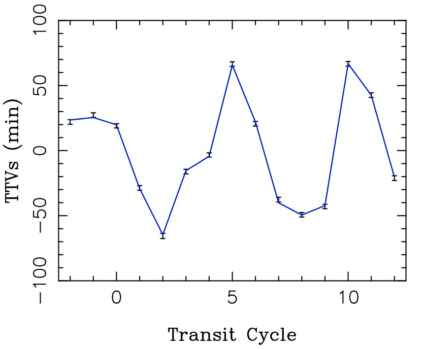
Figure 2: A more definitive fit to TTVs of KOI-872b. We had 15 transits in total in January 2012.

Yes, this was a critical assessment: TDVs of the 2nd solution should be smaller. Given that no TDVs were detected for KOI-872, the first solution can be ruled out because it generates TDVs in excess of the measurement errors.

By the way, my statement that “the 5:2 resonance … explains large TTVs” is incorrect. In fact, the large variations come from the 2:1 short-period term and are a consequence of the relatively large companion mass.

From David K’s email on 1/16/2012:

Awesome! I have more good news. There are three epochs missing in the data I sent you. My code had a bug where it cut them off, but I have fixed it now. So you have 3 new transits to add in.

From David N’s email on 1/17/2012:

Interesting news: The priority of the two solutions that I mentioned in the previous email switched with the new data. Now, the solution with a smaller planet near 5:3 gives chi2$=$5.8 (!) for 8 degrees of freedom. This one improved enormously. The solution with the Jupiter-mass planet near 5:2 now gives chi2=28.9, and can be rejected.

I am starting to be confident that we have finally obtained the correct and unique solution.

To summarize: In all likelihood we have here a system of two planets, the outer non-transiting planet should have mass about 25% lower than Saturn. It should be near the 5:3 resonance (period ratio 1.6967), low eccentricities and low inclinations.

We had 15 transits of KOI-872b and things were converging toward the solution near the 5:3 resonance, which is the correct one. And our excitement was building up…

From David K’s email on 1/17/2012:

Woah - that’s a hell of a fit!

Transit wise - interesting point. I can begin looking for transits on the 5:3 resonance. My immediate instinct is that it cannot be transiting given the planet is likely at least Neptune radius and should be sticking out like a sore thumb. I should be able to produce constraints on inclination vs radius for a fixed period which will give you a strong constraint to add in.

According to the best TTV/TDV fit mentioned above, the relative inclination of the two planets in the KOI-872 system must be small. We therefore considered the possibility that the outer planet might be transiting but was somehow overlooked. That turned out not to be the case: no transits of the outer planet were detected.

From David N’s email from 1/18/2012:

The short-period TTVs are sensitive to the Mc/M* ratio only, so I fit for Mc/M* and it comes out as $\sim$0.0002. For M*$=$0.8, this would roughly be a Saturn-mass planet.

It would be nice if transits of the 2nd planet can be ruled out. We could use it to give some lower limit on the perturbing planet’s inclination.

Good news: No interesting secondary maxima of chi2 popped out so far, so the two solutions that I mentioned in the previous email stand out as the only candidates. The 2nd solution can still be ruled out at >99% confidence, leading to a unique parameter set. :-)

With things going well, David K contacted the HEK team and told them the good news in the following email.

From David K’s email to the HEK team on 1/20/2012:

David N. and I have been working hard on HCV-439 these last few days are some answers are beginning to emerge. First of all, the new data strongly indicates the presence of star spots. Exomoon-like features seem to correlate with times of maximum activity which is a bad sign for exomoons. I have not run a moon fit through the new data yet, but my instincts are that this is not a moon.

However, the TTVs persist and exhibit a complex and highly significant signal. David N. has managed to obtain what appears to be a unique TTV inverse fit to the data. Let me just stress that this is the 1st time this has ever been done by anyone for a non-transiting perturber and represents a major accomplishment if the solution holds with our subsequent tests. It seems as though an outer planet of about 0.25 jupiter masses is near the 5:3 resonance and almost coaligned to the transiting planet.

The near-coalignment suggests the outer planet has a good chance of transiting, but not guaranteed. Indeed, the fact it is a Neptune sized planet suggests it should have already been detected if it was there. I have run a search through the data and Allan has manually checked for transits but there is nothing convincing in the data.

So we are thinking of running a paper on this system and I am working hard on finishing up all of the fits for this system. Perhaps we should arrange a telecon next week sometime to discuss everything. Including journal, naming of the system, confirming the system, etc.

It remained to confirm the planetary nature of KOI-872b. On the suggestion of David K, I performed a stability analysis with different masses of KOI-872b. The results are described in the following email.

From David N’s email to the HEK team on 1/30/2012:

I have done the stability test last week. The upper bound on Mb is 5 MJupiter for M*$=$0.8 Msun, which is clearly planetary. I can increase M* and see what happens. The result can be predicted from the Wisdom’s overlap criterion. Will update on this asap.

Please see attached a very preliminary draft of the paper that I sent to David K. already.

Given this result is so *cool* I think we should submit it to Science. I am now 99.9% sure that this is a real planetary system and that we identified the right solution. TTVs give us Mc/M*, Pc (or ac for assumed M*), ec$<$0.03, eb$<$0.02, ic$<$5 deg. We also have a very tight constraint on the pericenter and true longitudes.

Note that this is the first time that eccentricities were constrained from TTVs. The
inclination constraint is also unique. David K. just sent me new error estimates and things look even better that what is described in the attached draft.

The stellar mass of KOI-872 was later revised to $0.90\pm 0.04$ solar masses, indicating that the mass of KOI-872b cannot be larger than about 6 Jupiter masses.

We have done 17 iterations of the first draft and David K has written over 30 pages of the Supplementary Material. Gáspár Bakos, Lars Buchhave (Niels Bohr Institute) and Joel Hartman (Princeton University) improved the stellar parameters of KOI-872, and the whole HEK team was indispensable to the effort. Here it paid off how David K assembled the team with each member having a unique expertise. David was a driving force behind all efforts. He also found transits of a third planet in the KOI-872 system, a super-Earth with 1.7 Earth radius and 6.8-day period. This planet should produce TTVs of KOI-872b of the order of seconds and has nothing to do with the measured TTVs.

I performed innumerous additional test to demonstrate that no other solution, including polar/retrograde orbits and other absurd configurations, and systems of multiple planets, can compete with the solution already found. Dozens of different fits were attempted overall.

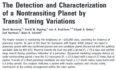
Figure 3: Header of our Science article that announced the discovery on July 1, 2012.

The paper was submitted to Science on 2/26/2012. We received three referee reports on 3/23/2012. This is from my email on 3/23/2012:

We received three *very* positive reviews!!! They are attached below.

Reviewer 1 praises the paper and has no criticism whatsoever. Referee 2 is similarly
enthusiastic and suggests only a few minor changes. Reviewer 3 liked the science as well (even congratulates us!) and offers numerous comments on how to improve the main text.

I have not seen such an uniformly positive reaction to any of the published Science/Nature papers that I contributed in the past. This is absolutely incredible and we should be proud of such an achievement.

The paper was finally published on June 1, 2012 (Figure 3), and David K and I prepared a press release to accompany the publication (Figure 4). To reflect the confirmed nature of these planets, the Kepler team later renamed this system to Kepler-46.

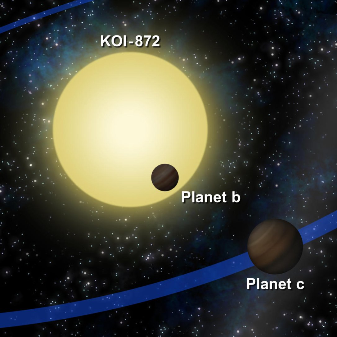
Figure 4: An illustration from the SwRI press release.

What is, in retrospect, the importance of this work in planetary? To answer this question, recall that TTVs were originally proposed as a non-transiting planet detection method, but prior to 2012 they have found more use in validating the transiting planet candidates from Kepler. A non-transiting planet has been previously inferred via TTVs, but the measurement was unable to support a unique solution (Ballard et al. 2011). Our Science article demonstrated the full potential of TTVs as a method to detect non-transiting planets and precisely characterize their properties. So, in some sense, the work on Kepler-46 closed the loop and recasted the TTVs as a planet-detection method.

This is useful because planetary transits can only be detected if the orbit is seen edge on. The transit method is therefore blind to planetary companions with even a small orbital tilt away from the line of sight. The TTV method, on the other hand, can be used to detect non-transiting companions (assuming that at least one planet in the system is transiting). TTVs can therefore play an important role in addressing the incompleteness of planetary systems detected from transits, with interesting implications for the distribution of mutual inclinations of orbits. Ultimately, all this links to the holy grail of the exoplanet research, which is to establish how planets form and evolve.

How confident are we about the Kepler-46 system characterization published in 2012? The full Kepler mission provided 35 transits of Kepler-46b (compared to 15 transits available to us back in 2012). My student, Ximena Saad-Olivera, recently performed a new TTV analysis with improved methods and all 35 transits (Saad-Olivera et al. 2017). This work confirmed that the Kepler-46c planet characterization, including its mass and orbital period, was correct. The orbital eccentricities of Kepler-46b and c favored by the new fits are slightly higher than the original estimates, $e_{b,c}\simeq 0.03$ versus $e_{b,c}\simeq 0.01$-0.015, but this is within the error bars reported in the original publication. Future TTV observations including those of the Transiting Exoplanet Survey Satellite (TESS), can be used to further improve the Kepler-46 parameters.

Unfortunately, the host star of Kepler-46 is not bright enough (apparent magnitude 15.3) for precise Doppler observations. For this reason, it may take some time before Kepler-46c is confirmed by independent means, be it the radial velocity technique or something else. At this point, however, I think this is a mere formality, which brings us to a related story of KOI-142 (Kepler-88).

We selected KOI-142 as an interesting TTV case from Mazeh et al. (2013), where they published a large collection of TTVs for dozens of Kepler candidates. The TTVs of KOI-142b are different from those of Kepler-46b in that they show a huge, nearly-sinusoidal signal ($\sim$12 hour amplitude, which is about 5% of the orbital period!). Also, we already had 105 transit epochs of KOI-142b in 2013.

I was initially not enthusiastic about this case, because KOI-142’s TTVs did not seem to have the type of complexity required for the unique inversion. I was wrong. When David K provided a detailed analysis of transits and I attempted the dynamical fits in early 2013, the code very rapidly converged to a single solution –an outer planet just outside the 2:1 resonance with KOI-142b– and nothing would move it from there.

This case is therefore unlike that of Kepler-46, where we only had a few transits to start with and were struggling with the solution ambiguity. Still, I did not understand why the solution should be unique in the case of KOI-142b until I realized that the measurements are so precise that they are picking up the chopping effect in the TTVs signal due to planet conjunctions (see Nesvorný & Vokrouhlický 2014 for discussion of the conjunction effect). The chopping effect has a very low amplitude, of the order of minutes, and was buried in the huge TTVs produced by the near 2:1 commensurability between orbits. The chopping effect has a high information content and this is what was driving the code to converge to a unique solution.

Another happy moment with KOI-142 happened when we predicted TDVs from the best-fit TTV solution and then went back to the transit photometry to dig out the TDVs of KOI-142b. The measured TDVs turned out to be exactly where the dynamical solution of TTVs was predicting them. Such things do not happen by chance.

Our paper on KOI-142 was published in ApJ (Nesvorný et al. 2013) and the system was later renamed to Kepler-88. Soon after, in 2014, new radial velocity measurements from the SOPHIE instrument were used to confirm the non-transiting planet Kepler-88c with the mass and orbital period that we previously inferred from TTVs (Barros et al. 2014; the published SOPHIE velocimetry was not precise enough to improve the original parameter determination). This firmly demonstrated that the TTV method can be used to detect and characterize non-transiting planets, and resolved many doubts that I had back in 2007 when I started working on this project. More detections and characterizations of non-transiting planets followed later (e.g., KOI-227, KOI-319 and KOI-882; Nesvorný et al. 2014).

Kepler-88 is interesting because of its dynamical configuration near the 2:1 resonance. The orbital period ratio of the two planets is 2.03. This is therefore one of many pairs of the Kepler planets with orbits just outside of a first-order resonance, but in this specific case we have a very good determination of masses and orbital eccentricities. It is possible that Kepler-88b and 88c migrated into the resonance by gravitational torques from their parent gas disk and later separated by tidal migration. For that, however, the tidal dissipation would have to be unusually strong. Also, the orbital eccentricity of the outer planet, Kepler-88c, is substantial ($0.056\pm 0.002$) and cannot be explained by gravitational perturbations from the inner planet. Perhaps there were, or still are, additional massive companions at larger orbital distances. In any case, the transits of Kepler-88b are predicted to disappear in 15-25 years from know (due to the precession of its orbital plane caused by Kepler-88c), so either these hypothetical outer companions reveal themselves in Kepler-88b’s TTVs within the next two decades or we will have to use other methods (e.g., precise radial velocity measurements) to figure things out.

References

- Agol et al. (2005) Agol, E., Steffen, J., Sari, R., Clarkson, W. 2005. On detecting terrestrial planets with timing of giant planet transits. Monthly Notices of the Royal Astronomical Society 359, 567-579.
- Ballard et al. (2011) Ballard, S., and 30 colleagues 2011. The Kepler-19 System: A Transiting 2.2 R⊕ Planet and a Second Planet Detected via Transit Timing Variations. The Astrophysical Journal 743, 200.
- Barros et al. (2014) Barros, S. C. C., and 11 colleagues 2014. SOPHIE velocimetry of Kepler transit candidates. X. KOI-142 c: first radial velocity confirmation of a non-transiting exoplanet discovered by transit timing. Astronomy & Astrophysics, Volume 561, 561.
- Feroz et al. (2009) Feroz, F., Hobson, M. P., Bridges, M. 2009. MULTINEST: an efficient and robust Bayesian inference tool for cosmology and particle physics. Monthly Notices of the Royal Astronomical Society 398, 1601-1614.
- Holman and Murray (2005) Holman, M. J., Murray, N. W. 2005. The Use of Transit Timing to Detect Terrestrial-Mass Extrasolar Planets. Science 307, 1288-1291.
- Holman et al. (2010) Holman, M. J., and 40 colleagues 2010. Kepler-9: A System of Multiple Planets Transiting a Sun-Like Star, Confirmed by Timing Variations. Science 330, 51.
- Kipping et al. (2012) Kipping, D. M., Bakos, G. Á., Buchhave, L., Nesvorný, D., Schmitt, A. 2012. The Hunt for Exomoons with Kepler (HEK). I. Description of a New Observational project. The Astrophysical Journal 750, 115.
- Mazeh et al. (2013) Mazeh, T., and 15 colleagues 2013. Transit Timing Observations from Kepler. VIII. Catalog of Transit Timing Measurements of the First Twelve Quarters. The Astrophysical Journal Supplement Series 208, 16.
- Nesvorný and Vokrouhlický (2014) Nesvorný, D., Vokrouhlický, D. 2014. The Effect of Conjunctions on the Transit Timing Variations of Exoplanets. The Astrophysical Journal 790, 58.
- Nesvorný et al. (2012) Nesvorný, D., Kipping, D. M., Buchhave, L. A., Bakos, G. Á., Hartman, J., Schmitt, A. R. 2012. The Detection and Characterization of a Nontransiting Planet by Transit Timing Variations. Science 336, 1133.
- Nesvorný et al. (2013) Nesvorný, D., Kipping, D., Terrell, D., Hartman, J., Bakos, G. Á., Buchhave, L. A. 2013. KOI-142, The King of Transit Variations, is a Pair of Planets near the 2:1 Resonance. The Astrophysical Journal 777, 3.
- Nesvorný et al. (2014) Nesvorný, D., Kipping, D., Terrell, D., Feroz, F. 2014. Photo-dynamical Analysis of Three Kepler Objects of Interest with Significant Transit Timing Variations. The Astrophysical Journal 790, 31.
- Saad-Olivera et al. (2017) Saad-Olivera, X., Nesvorný, D., Kipping, D. M., Roig, F. 2017. Masses of Kepler-46b,c from Transit Timing Variations. The Astronomical Journal 153, 198.