Average Weights and Power
in Weighted Voting Games

Abstract

We investigate a class of weighted voting games for which weights are randomly distributed over the standard probability simplex. We provide close-formed formulae for the expectation and density of the distribution of weight of the $k$-th largest player under the uniform distribution. We analyze the average voting power of the $k$-th largest player and its dependence on the quota, obtaining analytical and numerical results for small values of $n$ and a general theorem about the functional form of the relation between the average Penrose–Banzhaf power index and the quota for the uniform measure on the simplex. We also analyze the power of a collectivity to act (Coleman efficiency index) of random weighted voting games, obtaining analytical upper bounds therefor.

1 Introduction

An $n$–player weighted voting game $G$ is described by a weight vector $\mathbf{w}:=\left(w_{1},\dots,w_{n}\right)\in\Delta_{n}$, where $\Delta_{n}$ is the standard $\left(n-1\right)$–dimensional probability simplex, and a qualified majority quota $q\in\mathbb{(}\frac{1}{2},1\mathbb{]}$. In such a game, the set of winning coalitions $\mathcal{W\subset P}(V)$, where $V$ is the set of players, is defined as follows:

$$\mathcal{W}:=\bigg{\{}Q\subset V:\sum_{v\in Q}w_{v}\geq q\bigg{\}}.$$ (1)

We denote the set of all $n$-player weighted voting games by $\mathcal{G}_{n}$.

By random weighted voting game we mean a weighted voting game in which the number of players $n$ and the quota $q$ are fixed, and the weight vector $\mathbf{w}$ is drawn from the standard probability simplex $\Delta_{n}$ with some probability measure. Such games seem to be interesting for a number of reasons. First, the analysis of random weighted voting games enhances our understanding of weighted voting games in general. One of the major challenges in the field lies in the fact that generic results are usually rather difficult to obtain, while the behavior of weighted voting games in specific cases depends heavily on the characteristics of the specific weight vector and is often subject to number-theoretic peculiarities. For instance, some of the fundamental questions touch the relationship between the quota $q$ and the influence of individual players or efficiency of the system as a whole. Yet, for fixed weight vectors those dependencies are not only discontinuous, but highly erratic. Randomizing the weights, and thus averaging them over the simplex, smooths out the peculiarities of specific weight vectors, revealing hitherto unobserved regularities.

Second, randomizing the weights is likely to be of interest from the standpoint of voting rule design. Rule design tends to take place before players’ weights are fixed, and thus any predictions regarding the effects of the rules must, to the extent such effects depend on voting weights, necessarily be probabilistic. Also, just like players’ preferences are treated as random to abstract away from particular issues and focus the attention on the voting rules themselves (Roth, 1988), treating voting weights as random further abstracts away the particular configuration of players and brings other parameters (such as the number of players or the quota) into the forefront.

Obviously, the characteristics of a random weighted voting game depend on the choice of the probability measure. In the present article, we focus on the uniform (Lebesgue) measure (which is equivalent to the familiar Impartial Anonymous Culture Model used in computational social choice, see Kuga and Nagatani, 1974; Gehrlein and Fishburn, 1976). For that measure we obtain exact closed-form formulae for the expectation and density of the distribution of voting weight of the $k$–th largest player, an analytical formula for the expected values of product–moments of voting weights, a general theorem about the functional form of the relation between the expected values of the absolute and normalized Penrose–Banzhaf indices of the $k$–th largest player and the quota, the characteristic function of the distribution of coalition weights, and an approximation of the Coleman efficiency index (the power of a collectivity to act). All of those results constitute an original contribution of the paper. We further outline several applications of those results in the field of mathematical voting theory and in some other areas.

1.1 Related work

The notion of voting power, i.e., a player’s influence on the outcome of the game, which, as demonstrated by Penrose (1946), is not necessarily proportional to the player’s weight, is of fundamental importance to the study of voting systems. The two of the most popular voting power indices have been introduced by Shapley and Shubik (1954) and by Banzhaf (1964). Both define the voting power of a player $v$ in terms of the probability that their vote is decisive, but differ in their definition of the probability measure on the set of voting outcomes: the Shapley–Shubik index treats each permutation of players as equiprobable, while the Penrose–Banzhaf index assigns equal probabilities to all combinations of players. In addition, there are two versions of the Penrose–Banzhaf index in common use: one is defined as the probability of a player $v$ casting a decisive vote and is known as the non-normalized or absolute Penrose–Banzhaf index, $\psi_{v}$ (Dubey and Shapley, 1979), while the other one, $\beta_{v}$, is further normalized in order to ensure that the vector $\boldsymbol{\beta}:=\left(\beta_{1},\dots,\beta_{n}\right)$ lies in the probability simplex $\Delta_{n}$. Note that the vector of Shapley–Shubik indices always lies in $\Delta_{n}$, hence there is no need for further normalization.

It is well known that each player’s voting power depends not only on the weight vector, but also on the quota (Felsenthal and Machover, 1998; Leech and Machover, 2003). The relationship between the quota and the Penrose–Banzhaf power index for a fixed weight vector has been investigated by Leech (2002a) and more generally by Zuckerman et al. (2012), with the latter reporting several results on, inter alia, the upper and lower bounds of the ratio and difference between a player’s weight and their normalized Penrose–Banzhaf index. Analytical results about the values of the Penrose–Banzhaf index depending on the quota are available primarily for extreme quotas: the Penrose limit theorem (Penrose, 1946, 1952), proven under certain technical assumptions by Lindner and Machover (2004), provides that for $q=1/2$ and all $i,j\in V$, the ratio $\psi_{i}/\psi_{j}$ converges to $w_{i}/w_{j}$ as $n\rightarrow\infty$. On the other hand, it is easy to notice that as $q\rightarrow 1$, the values of $\psi_{i}$ and $\beta_{i}$ converge to $2^{1-n}$ and $1/n$, respectively, regardless of $\mathbf{w}$. Słomczyński and Życzkowski (2006, 2007) have established that $q^{\ast}:=\frac{1}{2}\left(1+(\sum_{i=1}^{n}w_{i}^{2})^{-1}\right)$ is a good approximation of the quota minimizing the distance $\left\|\mathbf{w}-\boldsymbol{\beta}\right\|_{2}$. For the discussion of the political significance of this quota, see Grimmett (2019). Therefore, if $\mathbf{w}$ is uniformly distributed on $\Delta_{n}$, then $\mathbb{E}(q^{\ast})\approx\frac{1}{2}+\frac{1}{\sqrt{\pi n}}$ (Życzkowski and Słomczyński, 2013). Upper bounds for the deviation between weights and Penrose–Banzhaf indices have been provided by Kurz (2018a). The relationship between the number of dummy players, i.e., such players $v$ that $\beta_{v}=0$, and the quota has been studied by Barthélémy et al. (2013).

The case of random weights has been investigated only for the Shapley–Shubik index $S_{v}$. The issue of selecting quotas maximizing and minimizing the Shapley–Shubik power of a given player is analyzed by Zick et al. (2011), who note that testing whether a given quota does so is an NP-hard problem. They also note that for a large range of quotas starting with $1/2$, the Shapley–Shubik power of a small player tends to be stable and close to their weight. Jelnov and Tauman (2014) established that if $\mathbf{w}$ is uniformly distributed on $\Delta_{n}$, the expected ratio of Shapley–Shubik index to weight approaches $1$ as $n\rightarrow\infty$. Bachrach et al. (2017) identify certain number-theoretic artifacts in the relationship between $S_{v}$ and $q$ for weights drawn from a multinomial distribution and normalized, and provides a lower bound for the expected index $S_{v}$ of the smallest player $v$. A problem similar to ours is posed by Filmus et al. (2016), who provide a closed-form characterization of the Shapley values of the largest and smallest players for $\mathbf{w}$ drawn from a uniform distribution on $\Delta_{n}$ or obtained by normalizing $n$ independent random variables drawn from a uniform distribution. Finally, Bachrach et al. (2016) give a closed-form formula for the Shapley–Shubik power index in games with super-increasing weights.

Numerous works analyze weighted voting games in a variety of empirical settings, including the Council of the European Union (Laruelle and Widgrén, 1998; Leech, 2002a; Felsenthal and Machover, 2004; Życzkowski and Cichocki, 2010; Życzkowski and Słomczyński, 2013), the U.S. Electoral College (Owen, 1975; Miller, 2013), the International Monetary Fund (Leech, 2002c; Leech and Leech, 2013), the U.N. Security Council (Strand and Rapkin, 2011) and joint stock companies (Leech, 2002b). The list of references is by no means complete, but demonstrates that the relevance of the subject goes far beyond purely academic.

2 Voting Weight of the $k$–th Largest Player

2.1 Introduction

Let $\Delta_{n}$ be the standard $\left(n-1\right)$–dimensional probability simplex, which represents the set of normalized weight vectors. We consider a random weighted voting game, where the weight vector $\mathbf{W}\in\Delta_{n}$ is a random variable with the uniform probability distribution, which will be thereafter denoted as $\mathop{\mathrm{U}nif}\left(\Delta_{n}\right)$. Since the uniform measure is symmetric, the players are indistinguishable a priori. But note that the coordinates of $\mathbf{W}$, i.e., the voting weights of the players, can almost surely be strictly ordered. This ordering provides a natural basis for distinguishing the players a posteriori.

Notation 1

For $k=1,\dots,n$ we denote the $k$–th largest coordinate of a vector $\mathbf{x}\in\mathbb{R}^{n}$ as $x_{k}^{\downarrow}$.

We start with the simplest question: what is the expected value and density of the distribution of voting weight of the $k$–th largest player in a random weighted voting game? While the coordinates of $\mathbf{W}$ can be thought of as a sample of random variables, and $W_{k}^{\downarrow}$ as the $k$–th largest order statistic of that sample, virtually all results in the field assume that order statistics are computed for a sample of independent variables, which is manifestly not the case for the barycentric coordinates of a vector drawn from a simplex. For that reason, the problem can be considered non-trivial.

2.2 Expected value: barycenter of the asymmetric simplex

Each ordering of the coordinates of a generic weight vector $\mathbf{w}$, $w_{1}^{\downarrow}>w_{2}^{\downarrow}>\dots>w_{n}^{\downarrow}$, corresponds to dividing the entire simplex $\Delta_{n}$ into $n!$ asymmetric parts and selecting one of them, which we will denote as $\tilde{\Delta}_{n}$. If $\mathbf{W}$ is drawn from the uniform distribution on $\Delta_{n}$, the ordered weight vector $\mathbf{W}^{\downarrow}=(W_{1}^{\downarrow},W_{2}^{\downarrow},\dots,W_{n}^{\downarrow})$ is uniformly distributed on the asymmetric simplex $\tilde{\Delta}_{n}$ with vertices $(1,0,\dots,0)$, $\frac{1}{2}(1,1,0,\dots,0)$, …, $\frac{1}{n}(1,1,\dots,1)$, see Fig. 1.

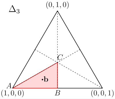
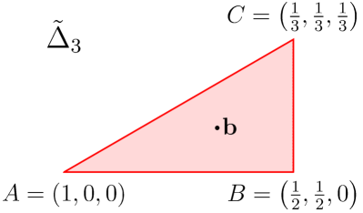
Figure 1: The case of $n=3$: probability simplex $\Delta_{3}$ as well as the asymmetric simplex ${\tilde{\Delta}_{3}}$ with vertices $A,B,C$ and the barycenter $\mathbf{b}=(A+B+C)/3=(11,5,2)/18$.

The expected value of $\mathbf{W}^{\downarrow}$ coincides with the barycenter $\mathbf{b}$ of $\tilde{\Delta}_{n}$. The $k$–th coordinate of that barycenter, $b_{k}$, for $k=1,\dots,n$, can be expressed by the sum of harmonic numbers $H_{l}:=\sum_{j=1}^{l}1/j$, as follows:

$$b_{k}=(H_{n}-H_{k-1})/n=\frac{1}{n}\sum_{j=k}^{n}\frac{1}{j}.$$ (2)

Thus we obtain an explicit formula, valid for an arbitrary number of players $n$, for the expected voting weight of the $k$–th largest player:

Proposition 2

If $\mathbf{W\sim}\mathop{\mathrm{U}nif}\left(\Delta_{n}\right)$, then for each$k=1,\dots,n$:

$$\mathbb{E}(W_{k}^{\downarrow})=b_{k}=\frac{1}{n}\sum_{j=k}^{n}\frac{1}{j}.$$ (3)

E.g., for $n=3$ the expected ordered random probability vector is $\mathbb{E}(\mathbf{W}^{\downarrow})=(11,5,2)/18$, while for $n=6$ one obtains $\mathbb{E}(\mathbf{W}^{\downarrow})=(147,87,57,37,22,10)/360$. Note that for a large $n$ the harmonic numbers scale as $\ln n+\gamma$, where $\gamma$ is the Euler–Mascheroni constant, so the first coordinate scales as $\ln n/n$, the median coordinate as $\ln 2/n$, and the smallest coordinate as $1/n^{2}$.

2.3 Densities

More generally, we obtain the following theorem, with proof given in the Appendix:

Theorem 3

If $\mathbf{W\sim}\mathop{\mathrm{U}nif}\left(\Delta_{n}\right)$, then $W_{k}^{\downarrow}$, $k=1,\dots,n$, is distributed according to an absolutely continuous distribution supported on $[1/n,1]$ for $k=1$ and on $[0,1/k]$ for $k>1$, with piecewise polynomial density $f_{n,k}:[0,1]\rightarrow\mathbb{R}$ given by:

$$f_{n,k}\left(x\right):=n(n-1)\dbinom{n-1}{k-1}\times\\ \sum\limits_{j=k}^{\min\left(n,\left\lfloor 1/x\right\rfloor\right)}(-1)^{j-k}\dbinom{n-k}{j-k}\left(1-jx\right)^{n-2}.$$ (4)

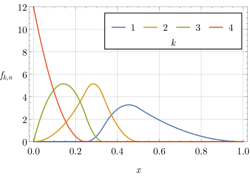
Figure 2: Densities of the distributions of the voting weight of the $k$-th largest of $4$ players for $k=1,\dots,4$.

Remark 4

The above result can also be obtained from results on the order statistics of uniform spacings (Darling, 1953; Rao and Sobel, 1980; Devroye, 1981). Nevertheless, we believe that the approach described in the Appendix is more promising in the context of a possible generalization to the family of Dirichlet distributions.

Remark 5

Elementary techniques of real analysis are sufficient to demonstrate that $f_{n,k}$ is smooth of class $\mathcal{C}^{n-3}$ for $n>2$.

Remark 6

Theorem 3 extends an earlier result by Qeadan et al. (2012), where, inter alia, closed-form formulae are obtained for the joint density of a sum and maximum of exponentially distributed i.i.d. random variables. It suffices to note that the normalized vector of $n$ independent exponential random variables with mean $1$ is uniformly distributed on $\Delta_{n}$ (Jambunathan, 1954).

Proposition 7

If $\mathbf{W\sim}\mathop{\mathrm{U}nif}\left(\Delta_{n}\right)$, then for $k=1,\dots,n$,

$$\left(W_{1}^{\downarrow},\dots,W_{n}^{\downarrow}\right)\overset{d}{=}\bigg{(}\sum_{j=1}^{n}\frac{W_{j}}{j},\dots,\sum_{j=n}^{n}\frac{W_{j}}{j}\bigg{)}.$$ (5)

Proof. By Jambunathan (1954) we can assume that for $j=1,\dots,n$,

$$W_{j}=\frac{X_{j}}{\sum_{i=1}^{n}X_{i}},$$ (6)

where $X_{1},\dots,X_{n}\sim\mathop{\mathrm{E}xp}\left(1\right)$ are independent random variables. Then by Rényi representation formula (Rényi, 1953),

$$\left(X_{1}^{\downarrow},\dots,X_{n}^{\downarrow}\right)\overset{d}{=}\bigg{(}\sum_{j=1}^{n}\frac{X_{j}}{j},\dots,\sum_{j=n}^{n}\frac{X_{j}}{j}\bigg{)}.$$ (7)

Moreover,

$$\sum_{k=1}^{n}X_{k}^{\downarrow}=\sum_{k=1}^{n}X_{k}=\sum_{k=1}^{n}\sum_{j=k}^{n}\frac{X_{j}}{j}.$$ (8)

Thus, from (7) and (8),

$$\bigg{(}\frac{X_{1}^{\downarrow}}{\sum_{i=1}^{n}X_{i}},\dots,\frac{X_{n}^{\downarrow}}{\sum_{i=1}^{n}X_{i}}\bigg{)}\overset{d}{=}\bigg{(}\frac{\sum_{j=1}^{n}\frac{X_{j}}{j}}{\sum_{i=1}^{n}X_{i}},\dots,\frac{\sum_{j=n}^{n}\frac{X_{j}}{j}}{\sum_{i=1}^{n}X_{i}}\bigg{)},$$ (9)

and by (6)

$$\bigg{(}\frac{\sum_{j=1}^{n}\frac{X_{j}}{j}}{\sum_{i=1}^{n}X_{i}},\dots,\frac{\sum_{j=n}^{n}\frac{X_{j}}{j}}{\sum_{i=1}^{n}X_{i}}\bigg{)}=\bigg{(}\sum_{j=1}^{n}\frac{W_{j}}{j},\dots,\sum_{j=n}^{n}\frac{W_{j}}{j}\bigg{)},$$ (10)

as desired.   

2.4 Product–moments of weights

Product–moments of voting weights are interesting for a number of reasons. Firstly, they appear in the definition of Rényi entropy (Rényi, 1961) of integer order $m$, where $m>1$, given by $-\ln\sum\nolimits_{i=1}^{n}w_{i}^{m}$. Secondly, we use them in Sec. 4 to obtain the characteristic function of the distribution of the total weight of a random coalition of players. Finally, the sum of squared weights appears in the definitions of the Herfindahl–Hirschman–Simpson index of diversity (Hirschman, 1945; Simpson, 1949; Herfindahl, 1950), $\sum\nolimits_{i=1}^{n}w_{i}^{2}$, the Laakso–Taagepera index of the effective number of players (Laakso and Taagepera, 1979; Taagepera and Grofman, 1981), $\left(\sum\nolimits_{i=1}^{n}w_{i}^{2}\right)^{-1}$, and the optimal quota minimizing the Euclidean distance between weight and power vectors (Słomczyński and Życzkowski, 2006, 2007), $\frac{1}{2}\left(1+(\sum_{i=1}^{n}w_{i}^{2})^{-1}\right)$.

We obtain a general theorem about the expected value of the product–moment of voting weights:

Theorem 8

If $\mathbf{W}\sim\mathop{\mathrm{U}nif}\left(\Delta_{n}\right)$, then for every $\mathbf{m}:=\linebreak\left(m_{1},\dots,m_{n}\right)\in\mathbb{N}^{n}$,

$$\mathbb{E}\bigg{(}\prod_{j=1}^{n}W_{j}^{m_{j}}\bigg{)}=\frac{\prod_{j=1}^{n}m_{j}!}{\left(n\right)_{\left|m\right|}},$$ (11)

where $\left|\mathbf{m}\right|:=\sum_{j=1}^{n}m_{j}$ and $\left(k\right)_{l}:=\prod_{j=0}^{l-1}(k+j)$.

Proof. Substituting $d=n-1$, $D=n$, and $l_{j}=x_{j}$ ($j=1,\dots,n$) for $\left(t_{1},\dots,t_{n}\right)\in\left(0,1\right)^{n}$ in Baldoni et al. (2011, Corollary 14) we obtain

$$\sum_{\mathbf{m}\in\mathbb{N}^{n}}\prod_{j=1}^{n}t_{j}^{m_{j}}\frac{\left(n\right)_{\left|\mathbf{m}\right|}}{\prod_{j=1}^{n}\left(m_{j}\right)!}\int_{\Delta_{n}}\prod_{j=1}^{n}x_{j}^{m_{j}}\,d\mathbf{x}=\frac{1}{\prod_{j=1}^{n}\left(1-t_{j}\right)}.$$ (12)

Expanding $\left(1-t_{j}\right)^{-1}$ into Taylor series, we get

$$\sum_{\mathbf{m}\in\mathbb{N}^{n}}\prod_{j=1}^{n}t_{j}^{m_{j}}\frac{\left(n\right)_{\left|\mathbf{m}\right|}}{\prod_{j=1}^{n}\left(m_{j}\right)!}\,\mathbb{E}\bigg{(}\prod_{j=1}^{n}W_{j}^{m_{j}}\bigg{)}=\sum_{\mathbf{m}\in\mathbb{N}^{n}}\prod_{j=1}^{n}t_{j}^{m_{j}}.$$ (13)

Then the assertion follows from the uniqueness of Taylor expansion.  

From this result, we obtain the following corollaries:

Corollary 9

If a random vector $\mathbf{W}\sim\mathop{\mathrm{U}nif}\left(\Delta_{n}\right)$, then for every $m\in\mathbb{N}_{+}$,

$$\mathbb{E}\bigg{(}\sum_{j=1}^{n}W_{j}^{m}\bigg{)}=\frac{m!}{\left(n+1\right)_{m-1}}.$$ (14)

Corollary 10

If a random vector $\mathbf{W}\sim\mathop{\mathrm{U}nif}\left(\Delta_{n}\right)$, then:

$$\mathbb{E}\bigg{(}\sum_{j=1}^{n}W_{j}^{2}\bigg{)}=\frac{2}{n+1},$$ (15)

and

$$\mathop{\mathrm{V}ar}\bigg{(}\sum_{j=1}^{n}W_{j}^{2}\bigg{)}=\frac{4\left(n-1\right)}{\left(n+1\right)^{2}\left(n+2\right)\left(n+3\right)}.$$ (16)

3 Voting Power of the $k$–th Largest Player

3.1 Definitions

The notion of a power index serves to characterize the a priori voting power of a player in a weighted voting game by measuring the probability that their vote will be decisive in a hypothetical ballot, i.e., the winning coalition would fail to satisfy the qualified majority condition if this player were to change their vote. In the classical approach by Penrose (1946, 1952) and Banzhaf (1964), it is assumed that all potential coalitions of players are equiprobable.

Let $\omega:=\left|\mathcal{W}\right|$ be the total number of winning coalitions, and for $i=1,\dots,n$, let $\omega_{i}:=\left|\left\{Q\in\mathcal{W}:i\in Q\right\}\right|$ be the number of winning coalitions that include the $i$–th player.

Definition 11

The absolute (non-normalized) Penrose–Banzhaf index $\psi_{i}$ of the $i$–th player, where $i=1,\ldots,n$, is the probability that the $i$–th player is decisive, i.e.,

$$\psi_{i}:=\frac{\omega_{i}-(\omega-\omega_{i})}{2^{n-1}}=\frac{2\omega_{i}-\omega}{2^{n-1}}.$$ (17)

To compare these indices for games with different numbers of players, it is convenient to define the normalized Penrose–Banzhaf index.

Definition 12

The normalized Penrose–Banzhaf index $\beta_{i}$ of the $i$–th player, where $i=1,\ldots,n$, is

$$\beta_{i}:=\frac{\psi_{i}}{\sum\nolimits_{j=1}^{n}\psi_{j}}.$$ (18)

The absolute Penrose–Banzhaf index, unlike the normalized one, has a clear probabilistic interpretation; however, for the latter the vector of indices always lies on $\Delta_{n}$.

3.2 Analytical results for very small values of $n$

For any $G,J\in\mathcal{G}_{n}$, let $I:V\left(G\right)\rightarrow V\left(J\right)$ be an isomorphism mapping the $k$–th largest player in $G$ to the $k$–th largest player in $J$ (assuming linear orderings of players in both games), and let $\sim$ be an equivalence relation on $\mathcal{G}_{n}$ such that $G\sim J$ if and only if $\mathcal{W}\left(G\right)=\mathcal{W}\left(J\right)$ up to isomorphism $I$. For small values of $n$, the elements of the quotient set $\mathcal{G}_{n}/\sim$ can be easily enumerated – see Muroga et al. (1962); Winder (1965); Muroga et al. (1970) and more generally Kirsch and Langner (2010); Barthélémy et al. (2011); Kurz (2012, 2018c). Their number increases rapidly with $n$: there are $2$ elements of $\mathcal{G}_{n}/\sim$ for $n=2$ players, $5$ for $3$ players, $14$ for $4$ players, $62$ for $5$ players, $566$ for $6$ players, and $11971$ for $7$ players.

For a fixed $q\in(\frac{1}{2},1]$ and for each $\chi\in\mathcal{G}_{n}/\sim$ there exists a set $L_{\chi}^{q}\subset\Delta_{n}$ such that for any point within $L_{\chi}^{q}$ the ordered power index vector $(\beta_{1}^{\downarrow},...,\beta_{n}^{\downarrow})$ equals $(\beta_{1}^{\chi},...,\beta_{n}^{\chi})$. Note that the volume of $L_{\chi}^{q}$ depends on the quota $q$. The expected voting power of the $k$–th largest player equals:

$$\mathbb{E}\left(\beta_{k}^{\downarrow}\right)=\sum_{\chi\in\mathcal{G}_{n}/\sim}\beta_{k}^{\chi}\,\lambda\left(L_{\chi}^{q}\right),$$ (19)

where by $\lambda$ we denote the Lebesgue measure on $\Delta_{n}$.

The case of $n=2$ is straightforward, as there are only two classes of games – the unanimity and the dictatorship of the largest player. Ordered power index vectors $(\beta_{1}^{\downarrow},\beta_{2}^{\downarrow})$ for those classes are equal to $(\frac{1}{2},\frac{1}{2})$ and $(1,0)$, respectively. Thus, we obtain:

$$\mathbb{E}\left(\beta_{1}^{\downarrow}\right)=2\left(\frac{1}{2}\lambda\Big{(}\big{(}\frac{1}{2},q\big{)}\Big{)}+\lambda\Big{(}\big{(}q,1\big{)}\Big{)}\right)=\frac{3}{2}-q,$$ (20a)

$$\mathbb{E}\left(\beta_{2}^{\downarrow}\right)=\lambda\Big{(}\big{(}\frac{1}{2},q\big{)}\Big{)}=q-\frac{1}{2}.$$ (20b)

Now let us consider the simplest non-trivial case – that of $n=3$. There are five elements of $\mathcal{G}_{n}/\sim$ to consider:

$\beta^{\chi}$ condition ($\chi$) probability ($\lambda\left(L_{\chi}^{q}\right)$) $(\frac{1}{3},\frac{1}{3},\frac{1}{3})$ $q>w_{1}^{\downarrow}+w_{2}^{\downarrow}$ $1-F_{3}(1-q)$ $(\frac{1}{2},\frac{1}{2},0)$ $w_{1}^{\downarrow}+w_{2}^{\downarrow}>q>w_{1}^{\downarrow}+w_{3}^{\downarrow}$ $F_{3}(1-q)-F_{2}(1-q)$ $(\frac{3}{5},\frac{1}{5},\frac{1}{5})$ $\begin{array}[]{c}(w_{1}^{\downarrow}+w_{3}^{\downarrow}>q>w_{2}^{\downarrow}+w_{3}^{\downarrow})\\ \wedge\,(w_{1}^{\downarrow}+w_{3}^{\downarrow}>q>w_{1}^{\downarrow})\end{array}$ $\!\!\!\begin{array}[]{c}(1-F_{1}(1-q))F_{1}(q)\\ -F_{1}(1-q)(1-F_{1}(q))\\ -1+F_{2}(1-q)\end{array}\!\!\!$ $(\frac{1}{3},\frac{1}{3},\frac{1}{3})$ $\begin{array}[]{c}(w_{2}^{\downarrow}+w_{3}^{\downarrow}>q)\\ \wedge\,(w_{1}^{\downarrow}<1/2)\end{array}$ $F_{1}(1-q)$ $(1,0,0)$ $(w_{1}^{\downarrow}>q)\wedge(w_{1}^{\downarrow}>1/2)$ $1-F_{1}(q)$

where by $F_{k}$ we denote the cumulative distribution of the $k$–th largest player’s weight, $k=1,2,3$.

From the above and (4), we obtain, see Fig. 3:

$\qquad\lambda\left(L_{\chi}^{q}\right)$ $\beta^{\chi}$ $\quad\qquad q\leq 2/3\qquad\quad$ $\quad\qquad q\geq 2/3\qquad\quad$ $(\frac{1}{3},\frac{1}{3},\frac{1}{3})$ $0$ $9q^{2}-12q+4$ $(\frac{1}{2},\frac{1}{2},0)$ $12q^{2}-12q+3$ $-15q^{2}+24q-9$ $(\frac{3}{5},\frac{1}{5},\frac{1}{5})$ $-24q^{2}+30q-9$ $3q^{2}-6q+3$ $(\frac{1}{3},\frac{1}{3},\frac{1}{3})$ $9q^{2}-12q+4$ $0$ $(1,0,0)$ $3q^{2}-6q+3$ $3q^{2}-6q+3$

At this point, from (19) we get:

$$\mathbb{E}\left(\beta_{1}^{\downarrow}\right) =\begin{cases}\frac{12}{5}(q-q^{2})+\frac{1}{30},&q\leq 2/3,\\ \frac{1}{10}(16-16q+3q^{2})+\frac{1}{30},&q\geq 2/3,\end{cases}$$ (21a)

$$\mathbb{E}\left(\beta_{2}^{\downarrow}\right) =\begin{cases}\frac{21}{5}q^{2}-4q+1+\frac{1}{30},&q\leq 2/3,\\ \frac{1}{10}(68q-39q^{2}+26),&q\geq 2/3,\end{cases}$$ (21b)

$$\mathbb{E}\left(\beta_{3}^{\downarrow}\right) =\begin{cases}-\frac{9}{5}q^{2}+2q-\frac{1}{2}+\frac{1}{30},&q\leq 2/3,\\ \frac{2}{5}(9q^{2}-13q)+2+\frac{1}{30},&q\geq 2/3.\end{cases}$$ (21c)

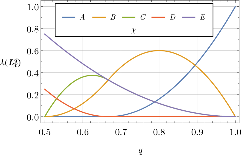
Figure 3: Probabilities of the five classes of games $\chi\in\mathcal{G}_{3}/\sim$ as a function of the quota $q$. Classes $A$, $B$, $C$, $D$, and $E$ correspond, respectively, to weight vectors $\beta^{A}:=(\frac{1}{3},\frac{1}{3},\frac{1}{3})$, $\beta^{B}:=(\frac{1}{2},\frac{1}{2},0)$, $\beta^{C}:=(\frac{3}{5},\frac{1}{5},\frac{1}{5})$, $\beta^{D}:=(\frac{1}{3},\frac{1}{3},\frac{1}{3})$, and $\beta^{E}:=(1,0,0)$.

3.3 Numerical results for small values of $n$

As mentioned in Sec. 1, if a player’s voting weight is fixed, the dependence of the voting power on the quota $q\in(\frac{1}{2},1]$ seems to be highly erratic. This is illustrated by Figure 4.

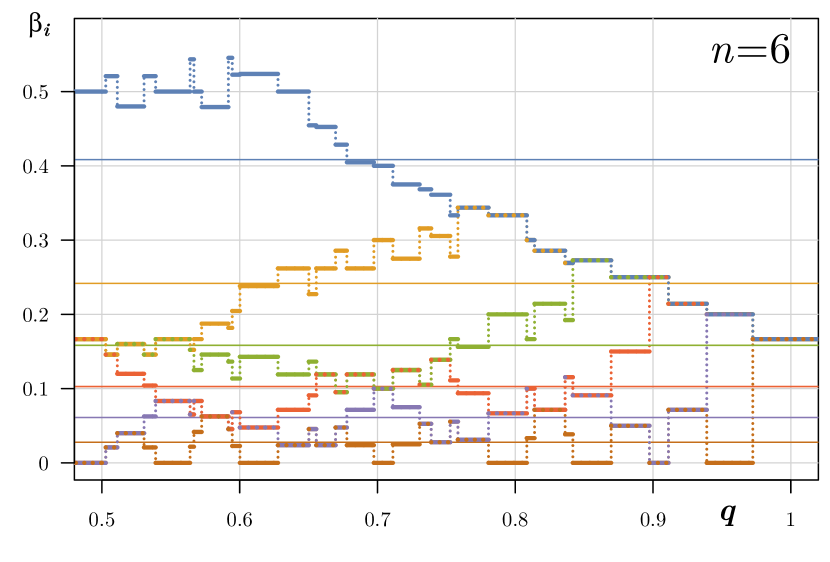
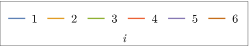
Figure 4: Normalized Penrose–Banzhaf power indices $\beta_{1},\dots,\beta_{6}$ in a six-player weighted voting game with weights fixed at the barycenter of the asymmetric simplex, ${\mathbf{b}}=(147,87,57,37,22,10)/360$, as functions of the quota $q$. Horizontal lines represent the voting weights of each player. An earlier version of this figure appeared in Rzażewski et al. (2014, p. 282), cf. Fig. 5.

On Fig. 5 we plot numerical estimates of $\mathbb{E(}\beta_{k}^{\downarrow})$ and $\mathbb{E(}\psi_{k}^{\downarrow})$ as functions of $q$, obtained by Monte Carlo samplings of $2^{16}$ random vectors of length $n=3,6,9$. Their examination reveals certain general regularities.

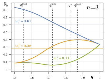
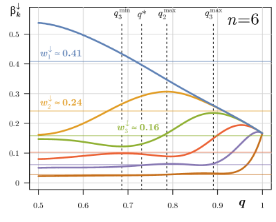
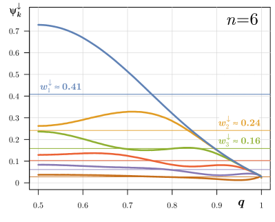
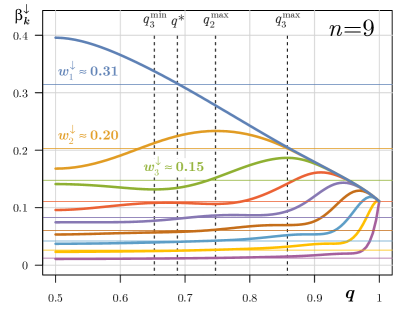
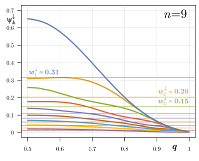
Figure 5: Absolute and normalized Penrose–Banzhaf power indices of $n$ players averaged over the probability simplex $\Delta_{n}$ with respect to the uniform measure as functions of the quota $q$. Horizontal lines represent the average voting weight of each player. The vertical line $q=q^{*}$ represents the approximation of the quota minimizing the distance $\left\|\mathbf{w}-\boldsymbol{\beta}\right\|_{2}$, see Życzkowski and Słomczyński (2013). An earlier version of one of the figures appeared in Rzażewski et al. (2014, p. 287).

For $q\rightarrow 1/2$ the average voting power of the largest player, $\mathbb{E(}\beta_{1}^{\downarrow})$, is considerably greater than their average weight, $\mathbb{E(}w_{1}^{\downarrow})$, at the expense of all the other players, and then decreases monotonically with the quota $q$. The second player initially loses the most, but their average voting power, $\mathbb{E(}\beta_{2}^{\downarrow})$, increases up to its single maximum, $q_{2}^{\max}$, while the average voting power of the third player, $\mathbb{E(}\beta_{3}^{\downarrow})$, has two extrema, $q_{3}^{\min}$ and $q_{3}^{\max}$. The average voting power of small players initially fluctuate mildly with $q$ around their average weights, with the amplitudes of these fluctuations diminishing as $k$ increases, and for $q\rightarrow 1$ the voting powers of all players converge to $1/n$.

Careful examination of the numerical results suggests a following conjecture:

Conjecture 13

For the uniform distribution on the probability simplex $\Delta_{n}$ and for every $k=1,...,n$, the average normalized Penrose–Banzhaf power index of the $k$–th largest player, $\mathbb{E}(\beta_{k}^{\downarrow})$, has exactly $k-1$ local extrema over $(1/2,1)$ as a function of $q$.

Remark 14

Note that for $n=3$, Conjecture 13 follows immediately from the analytic form of $\mathbb{E}(\beta_{k}^{\downarrow})$ given by (21). The voting power of the second largest player, $\mathbb{E(}\beta_{2}^{\downarrow})$, admits a maximal value at $q_{2}^{\max}=34/39$ $(\approx 87.18\%)$, while $\mathbb{E(}\beta_{3}^{\downarrow})$ exhibits a minimum at $q_{3}^{\min}=5/9$ $(\approx 55.56\%)$ and a maximum at $q_{3}^{\max}=13/18$ $(\approx 72.22\%)$.

4 The power of a collectivity to act

The power of a collectivity to act, i.e., the ease of reaching a decision, is usually measured with the Coleman efficiency index (Coleman, 1971), defined as the probability that a random coalition $Q\in\mathcal{P}(V)$ is a winning one:

$$C:=\frac{\omega}{2^{n}},$$ (22)

where $\omega:=\left|\mathcal{W}\right|$.

Remark 15

Note that $C$ is a decreasing function of the quota $q\in(\frac{1}{2},1]$. Since it is impossible for any coalition $Q\in\mathcal{P}(V)$ that both $Q$ and $V\setminus Q$ be winning, $C\leq\frac{1}{2}$. On the other hand, $C\geq C\left(1\right)=2^{-\left|\left\{j\,=\,1,\dots,n~{}:~{}w_{j}>0\right\}\right|}.$

Let $\mu_{n}$ be the Bernoulli measure on $\left\{0,1\right\}^{n}$, and let $Z:\Delta_{n}\times\left\{0,1\right\}^{n}\rightarrow\mathbb{R}$ be given by the formula $Z\left(\mathbf{w},\mathbf{\xi}\right):=\sum_{i=1}^{n}w_{i}\xi_{i}-\frac{1}{2}$, where $\mathbf{w}\in\Delta_{n}$ and $\mathbf{\xi}\in\left\{0,1\right\}^{n}$. Note that

$$\mathbb{E}_{\lambda\times\mu_{n}}\left(C\right)=1-F_{Z}\left(q-\frac{1}{2}\right),$$ (23)

where $\lambda$ is the Lebesgue measure on $\Delta_{n}$, and $F_{Z}$ is the distribution function of $Z$ with respect to the probability measure $\lambda\times\mu_{n}$ on $\Delta_{n}\times\left\{0,1\right\}^{n}$. This distribution function can be calculated by the following proposition:

Theorem 16

The characteristic function of $Z$ is given by

$$\varphi_{Z}\left(t\right)={}_{1}\digamma_{2}\left(\begin{array}[]{c}n\\ \frac{1}{2}+\frac{n}{2},\frac{n}{2}\end{array};-\left(\frac{t}{4}\right)^{2}\right),$$ (24)

for $t\in\mathbb{R}$, where ${}_{1}\digamma_{2}$ is a generalized hypergeometric function.

Proof. For a fixed $\mathbf{w}\in\Delta_{n}$ and $k=1,\dots,n$, let $X_{k}:=w_{k}(\xi_{k}-\frac{1}{2})$ and $X:=\sum_{k=1}^{n}X_{k}$. Then for $t\in\mathbb{R}$,

$$\varphi_{X_{k}}\left(t\right)=\frac{1}{2}\left(e^{\frac{1}{2}itw_{k}}+e^{-\frac{1}{2}itw_{k}}\right)=\cos\left(\frac{tw_{k}}{2}\right),$$ (25)

and

$$\varphi_{X}\left(t\right) =\prod_{k=1}^{n}\cos\left(\frac{tw_{k}}{2}\right)=\sum_{j=0}^{\infty}\frac{t^{j}}{j!}\left.\frac{d^{j}}{dt^{j}}\prod_{k=1}^{n}\cos\left(\frac{tw_{k}}{2}\right)\right|_{t=0}$$

$$=\sum_{j=0}^{\infty}\frac{t^{2j}}{\left(2j\right)!}\sum_{j_{1}+\ldots+j_{n}=j}\left(-1\right)^{j}\,2^{-2j}\left(2j\right)!\prod_{k=1}^{n}\frac{w_{k}^{2j_{k}}}{\left(2j_{k}\right)!}$$

$$=\sum_{j=0}^{\infty}\left(-1\right)^{j}\left(\frac{t}{2}\right)^{2j}\sum_{j_{1}+\ldots+j_{n}=j}\prod_{k=1}^{n}\frac{w_{k}^{2j_{k}}}{\left(2j_{k}\right)!}.$$ (26)

It can be shown that the resulting series is absolutely convergent. Hence, and by Theorem 8,

$$\varphi_{Z}\left(t\right) =\int_{\Delta_{n}}\varphi_{X}\left(t\right)\,d\lambda$$

$$=\sum_{j=0}^{\infty}\left(-1\right)^{j}\left(\frac{t}{2}\right)^{2j}\sum_{j_{1}+\ldots+j_{n}=j}\frac{\mathbb{E}\left(\prod_{k=1}^{n}W_{k}^{2j_{k}}\right)}{\prod_{k=1}^{n}\left(2j_{k}\right)!}$$

$$=\sum_{j=0}^{\infty}\left(-1\right)^{j}\left(\frac{t}{2}\right)^{2j}\frac{1}{\left(n\right)_{2j}}\binom{j+n-1}{n-1}$$

$$={}_{1}\digamma_{2}\left(\begin{array}[]{c}n\\ \frac{1}{2}+\frac{n}{2},\frac{n}{2}\end{array};-\left(\frac{t}{4}\right)^{2}\right),$$ (29)

as desired.

 

Thus by numerical inversion of the characteristic function $\varphi_{Z}$, we can easily estimate the expected Coleman efficiency index $\mathbb{E}_{\lambda\times\mu_{n}}(C)$ for any quota $q\in(\frac{1}{2},1]$. The results for a number of arbitrarily chosen values of $n$ are plotted on Fig. 6.

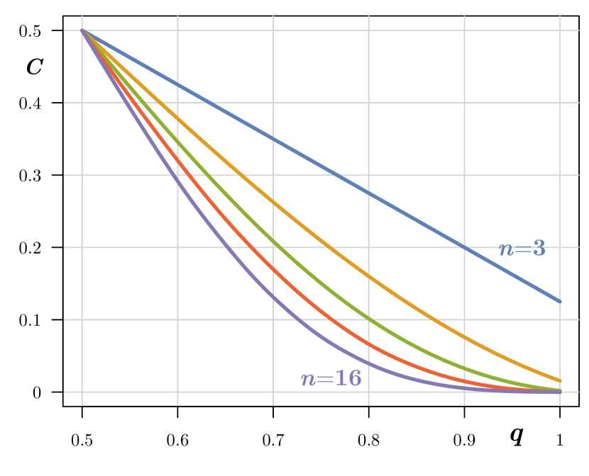
Figure 6: Coleman efficiency indices $C$ of weighted voting games with $n=3,6,9,12,16$, averaged in each case over $\Delta_{n}$ with respect to the uniform measure, as functions of the quota $q$.

The following results provide analytical formulae for, respectively, the upper bound and the asymptotic approximation of the Coleman efficiency index.

Remark 17

Let $\mathbf{W}\sim\mathop{\mathrm{U}nif}\left(\Delta_{n}\right)$. By the central limit theorem and (23), the expected Coleman efficiency index, $\mathbb{E}_{\lambda\times\mu_{n}}\left(C\right)$, can be approximated for fixed $n$ and $q$ by

$$C_{1}:=1-\Phi\left(\sqrt{2\left(n+1\right)}\left(q-\frac{1}{2}\right)\right),$$ (30)

where $\Phi$ is the standard normal cumulative distribution function. The upper bound for the approximation error can be obtained from the Berry–Esseen theorem (Berry, 1941; Esseen, 1942). However, numerical simulations suggest that it exceeds the actual approximation error by several orders of magnitude.

The above approximation is particularly useful when one is interested in finding such value of $q$ as to obtain a specific expected Coleman efficiency index, see Fig. 7.

\begin{overpic}[width=433.62pt]{colemanErr.pdf} \put(45.0,62.0){\includegraphics[width=128.0374pt]{legend3.pdf}} \end{overpic}

Figure 7: Error ratio $r$ of the approximation (30) of the expected Coleman efficiency index in random weighted voting games with $n=4,6,9,12$, where $r(y):=C_{1}^{-1}(y)/(\mathbb{E}(C))^{-1}(y)=C^{-1}_{1}(\mathbb{E}(C)(q))/q$ for $y=\mathbb{E}(C)(q)\in[2^{-2n},2^{-1}]$.

For any fixed weight vector $\mathbf{w}$, we have the following upper bound for the Coleman efficiency index $C$:

Proposition 18

In a weighted voting game with $q\geq 1/2$ the Coleman efficiency index $C$ is bounded from the above in the following manner:

$$C\leq\exp\left(-\frac{2\left(q-1/2\right)^{2}}{\sum_{i=1}^{n}w_{i}^{2}}\right).$$ (31)

Proof. A proof follows from the Hoeffding’s inequality (Hoeffding, 1963). If $Y_{1},\dots,Y_{n}$ are independent random variables such that $Y_{i}$ is almost surely bounded by $\left[\tau_{i}^{-},\tau_{i}^{+}\right]$ for every $i=1,\dots,n$, then for any $h\geq 0$:

$$\Pr\left(\sum_{i=1}^{n}\left(Y_{i}-\mathbb{E}\left(Y_{i}\right)\right)\geq h\right)\leq\exp\left(\frac{-2h^{2}}{\sum_{i=1}^{n}\left(\tau_{i}^{+}-\tau_{i}^{-}\right)^{2}}\right).$$ (32)

Putting $\Pr=\mu_{n}$, $Y_{i}=w_{i}\xi_{i}$, $h=q-1/2$, $\tau_{i}^{+}=w_{i}$ and $\tau_{i}^{-}=0$, we obtain Proposition 18.   

5 Splines

Any quantity that is a function of the weighted voting game (e.g., the Coleman efficiency index, the Penrose–Banzhaf and Shapley–Shubik power indices, etc.), averaged over the probability simplex $\Delta_{n}$, and considered as a function of the quota, has the following property:

Theorem 19

Let $U:\Delta_{n}\times(\frac{1}{2},1]\rightarrow\mathcal{G}_{n}$ be a function mapping a weight vector and a quota to the related weighted voting game. If $\mathbf{W}\sim\mathop{\mathrm{U}nif}\left(\Delta_{n}\right)$, then for any $p:\mathcal{G}_{n}\rightarrow\mathbb{R}$,

$$(1/2,1]\ni q\rightarrow\mathbb{E}\left(p\left(U\left(\mathbf{W},q\right)\right)\right)\in\mathbb{R}$$ (33)

is a spline of degree at most $n-1$.

Proof. Note that $\left(\Delta_{n}\times(1/2,1]\right)/\ker U$ is a partition of the polytope $\Delta_{n}\times(1/2,1]$ into blocks

$$P_{G}:=\left\{(\mathbf{w,}q\mathbf{)}\in\Delta_{n}\times(1/2,1]:U\left(\mathbf{w},q\right)=G\right\}$$ (34)

for $G\in\mathcal{G}_{n}$. Each $P_{G}$ is a convex polytope (Grünbaum et al., 2003, ch. 2), since it can be described by a system of $2^{n}$ linear inequalities with one inequality for each coalition $Q\in\mathcal{P}(V)$, corresponding to the condition that $Q$ be winning or losing, i.e., that $\left\langle\boldsymbol{1}_{Q},\mathbf{w}\right\rangle\geq q$ if $Q\in G$ and $\left\langle\boldsymbol{1}_{Q},\mathbf{w}\right\rangle\leq q$ if $Q\notin G$ (Mason and Parsley, 2016). For every $G\in\mathcal{G}_{n}$, and $q\in(\frac{1}{2},1]$, the intersection of $P_{G}$ and an affine hyperplane $\Theta_{q}:=\{\mathbf{x}\in\mathbb{R}^{n}:\left\langle\mathbf{1},\mathbf{x}\right\rangle=1\}\times\{q\}$ parallel to $\Delta_{n}$, is called the weight polytope $P_{G}^{q}$ (Kurz, 2018b).

For any $p:\mathcal{G}_{n}\rightarrow\mathbb{R}$, let $q\in(1/2,1]$ be fixed. Clearly, $p\left(U\left(\mathbf{W},q\right)\right)$ is constant over $P_{G}^{q}$ for each $G\in\mathcal{G}_{n}$. Thus, $\mathbb{E}\left(p\left(U\left(\mathbf{W},q\right)\right)\right)$ is an affine combination of the volumes of weight polytopes:

$$\mathbb{E}\left(p\left(U\left(\mathbf{W},q\right)\right)\right)=\sum_{G\in\mathcal{G}_{n}}p\left(G\right)\,\lambda\left(P_{G}^{q}\right),$$ (35)

where $\lambda$ is the Lebesgue measure on $\Delta_{n}\times\left\{q\right\}$. It is well–known that the volume of an intersection of an $n$–polytope $P$ and a moving hyperplane $\Theta_{t}$ sweeping $P$ over some interval $\left(t_{0},t_{1}\right)\subset\mathbb{R}$ is a piecewise polynomial function (spline) of $t$ of degree at most $n-1$ (De Boor and Höllig, 1982; Bieri and Nef, 1983; Lawrence, 1991; Gritzmann and Klee, 1994, Theorem 3.2.1). Thus, $\mathbb{E}\left(p\left(U\left(\mathbf{W},\cdot\right)\right)\right)$ is a sum of splines of degree at most $n-1$, and accordingly also a spline of the same or lower degree.   

6 Concluding remarks

In the present article we obtain a number of new analytical results, including explicit formulae for the expected value and density of the voting weight of the $k$–th largest player in a random weighted voting game, and for the expected values of product–moments of voting weights, a characteristic function of the distribution of the total weight of a random coalition of players, and a general theorem about the functional form of the relation between any quantity that is a function of the weighted voting game and the quota. In addition, we note several regularities appearing in numerical simulations that seem to provide promising subjects for further study.

The results presented above enhance our understanding of the relationship between voting game parameters, such as the Coleman efficiency index or voting power, and the qualified majority quota $q$ in random voting games where weights are drawn from the uniform distribution on the probability simplex $\Delta_{n}$. These can have potential applications in the area of voting rule design, especially if the rules are drafted behind a veil of ignorance with regard to the actual distribution of players’ weights (as is the case for business corporations). Moreover, the results presented in Sec. 2, regarding the distribution of voting weights of the $k$–th largest player and the expected values of product–moments of voting weights, may find applications in other areas of social choice theory. For instance, Theorem 3 can be applied to obtain the probability of a candidate with a specified vote share winning the election held under the plurality rule.

Future work will focus on proving Conjecture 13; developing a workable large–$n$ approximation on the basis of the normal approximation of the Penrose–Banzhaf index; and generalizing the results presented here for other Dirichlet measures.

Appendix. Proof of Theorem 3

Let $X_{1},\dots,X_{n}\sim\mathop{\mathrm{E}xp}\left(1\right)$ be independent random variables with densities $f_{X_{j}}\left(x\right):=e^{-x}$ for every $j=1,\dots,n$ and $x>0$. As in the proof of Proposition 7, we can assume that

$$W_{k}^{\downarrow}=\frac{X_{k}^{\downarrow}}{\sum_{i=1}^{n}X_{i}}.$$ (36)

By David and Nagaraja (2003, (2.1.3)), the order statistic $X_{k}^{\downarrow}$ ($k=1,\dots,n$) has an absolutely continuous distribution with the density given, for $x\in\mathbb{R}_{+}$, by

$$f_{X_{k}^{\downarrow}}(x)=k\dbinom{n}{k}e^{-kx}\left(1-e^{-x}\right)^{n-k}.$$ (37)

Let $\Psi:=\sum\nolimits_{j=1}^{n}X_{j}$. By the Markov property of order statistics (David and Nagaraja, 2003, Thm. 2.5), the conditional distribution of $X_{1}^{\downarrow},\dots,X_{k-1}^{\downarrow}$ given $X_{k}^{\downarrow}=y>0$, is the same as the distribution of order statistics $Y_{1}^{\downarrow},\dots,Y_{k-1}^{\downarrow}$ from i.i.d. random variables $Y_{1},\dots,Y_{k-1}$ with $Y_{j}\sim\mathop{\mathrm{E}xp}\left(1\right)$ truncated to $(y,\infty)$ for $j=1,\dots,k-1$. Likewise, the conditional distribution of $X_{k+1}^{\downarrow},\dots,X_{n}^{\downarrow}$ given $X_{k}^{\downarrow}=y>0$, is identical to the distribution of order statistics $Z_{1}^{\downarrow},\dots,Z_{n-k}^{\downarrow}$ from i.i.d. random variables $Z_{1},\dots,Z_{n-k}$ such that $Z_{j}\sim\mathop{\mathrm{E}xp}\left(1\right)$ truncated to $(0,y)$ for $j=1,\dots,n-k$. Moreover, we can choose $Y_{1},\dots,Y_{k-1}$ and $Z_{1},\dots,Z_{n-k}$ to be independent. Thus, for their sums we obtain respectively:

$$\left(\left(\sum_{j=1}^{k-1}X_{j}^{\downarrow}\right)\Bigg{|}X_{k}^{\downarrow}=y\right)\overset{d}{=}\sum_{j=1}^{k-1}Y_{j}^{\downarrow}\overset{d}{=}\sum_{j=1}^{k-1}Y_{j},$$ (38)

i.e., the sum of $k-1$ independent exponential random variables variables truncated to $(y,\infty)$, and

$$\left(\left(\sum_{j=k+1}^{n}X_{j}^{\downarrow}\right)\Bigg{|}X_{k}^{\downarrow}=y\right)\overset{d}{=}\sum_{j=1}^{n-k}Z_{j}^{\downarrow}\overset{d}{=}\sum_{j=1}^{n-k}Z_{j},$$ (39)

i.e., the sum of $n-k$ independent exponential random variables truncated to $(0,y)$. But it is easy to see that a sum of $k-1$ left–truncated independent exponential random variables is a gamma–distributed random variable with parameters $\left(k-1,1\right)$ shifted by a constant, $y\left(k-1\right)$. Thus,

$$\left(\Psi\bigg{|}X_{k}^{\downarrow}=y\right)=\left((\Psi-X_{k}^{\downarrow})\bigg{|}X_{k}^{\downarrow}=y\right)+y\overset{d}{=}\Xi,$$ (40)

where $\Xi:=\sum_{j=1}^{k-1}Y_{j}+yk+\sum_{j=1}^{n-k}Z_{j}$, and $\sum_{j=1}^{k-1}Y_{j}\sim\mathop{\mathrm{G}amma}\left(k-1,1\right)$ is independent of $Z_{1},\dots,Z_{n-k}$. Hence, the characteristic function of their sum is given by the product of the characteristic functions:

$$\varphi_{\sum_{j=1}^{k-1}Y_{j}}\left(t\right):=\left(1-it\right)^{-(k-1)},$$ (41)

for $t\in\mathbb{R}$, and

$$\varphi_{Z_{j}}\left(t\right) :=\frac{e^{y}}{1-e^{-y}}\int_{0}^{y}e^{itx-x}dx$$

$$=\left(1-it\right)^{k-n}\,\left(\frac{e^{y}-e^{ity}}{e^{y}-1}\right)^{n-k},$$ (42)

for $t\in\mathbb{R}$ and $j=1,\dots,n-k$. Accordingly,

$$\varphi_{\Xi}\left(t\right)=\left(1-it\right)^{1-n}\left(\frac{e^{y}-e^{ity}}{e^{y}-1}\right)^{n-k}\,e^{ityk},$$ (43)

Applying the binomial theorem, we obtain

$$\varphi_{\Xi}(t)=(e^{y}-1)^{k-n}\times\\ \sum\limits_{l=k}^{n}\dbinom{n-k}{l-k}\left(1-it\right)^{1-n}e^{y(n-l)}e^{i\pi(l-k)}e^{ityl}.$$ (44)

As $\varphi_{\Xi}$ is integrable, for every $x\in\mathbb{R}_{+}$ we obtain by Lévy’s inversion formula (Billingsley, 1995, p. 347, (26.20)):

$$f_{\Xi}(x)=\frac{1}{2\pi}\int_{-\infty}^{+\infty}e^{-itx}\varphi_{\Xi}(t)\,dt=\frac{1}{2\pi}(e^{y}-1)^{k-n}\times\\ \sum\limits_{l=k}^{n}\left(-1\right)^{l-k}\dbinom{n-k}{l-k}e^{y(n-l)}\mathcal{\tciFourier}\left\{\left(1-it\right)^{1-n}\right\}(x-yl).$$ (45)

By Bateman (1954, § 3.2 (3), p. 118), we have

$$\mathcal{\tciFourier}\left\{\left(1-it\right)^{1-n}\right\}(s)=\left\{\begin{array}[]{cc}\frac{2\pi s^{n-2}e^{-s}}{\Gamma\left(n-1\right)},&\qquad s>0,\\ 0,&\qquad s\leq 0.\end{array}\right.$$ (46)

From (40), (45), and (46),

$$f_{\Psi|X_{k}^{\downarrow}\,=\,y}(x)=f_{\Xi}\left(x\right)=(e^{y}-1)^{k-n}\times\\ \sum\limits_{l=k}^{\min\left(n,\left\lfloor x/y\right\rfloor\right)}\frac{\left(-1\right)^{l-k}}{\left(n-2\right)!}\dbinom{n-k}{l-k}\left(x-yl\right)^{n-2}e^{ny-x}.$$ (47)

Thus, by Curtiss (1941), the density of the ratio is given by

$$f_{W_{k}^{\downarrow}}\left(x\right)=\int_{0}^{\infty}\left|z\right|\,f_{X_{k}^{\downarrow},\Psi}(xz,z)\,dz$$

$$=\int_{0}^{\infty}\left|z\right|\,f_{\Psi|X_{k}^{\downarrow}\,=\,xz}(z)\,f_{X_{k}^{\downarrow}}(xz)\,dz$$

$$=\int_{0}^{\infty}\left|z\right|\sum\limits_{l=k}^{T(n,x)}\frac{k\left(-1\right)^{l-k}}{\left(n-2\right)!}\dbinom{n-k}{l-k}\dbinom{n}{k}\frac{\left(z-xzl\right)^{n-2}}{e^{z}}\,dz$$

$$=\frac{k}{\left(n-2\right)!}\sum\limits_{l=k}^{T(n,x)}\Gamma\left(n\right)\dbinom{n-k}{l-k}\dbinom{n}{k}\frac{\left(-1\right)^{l-k}}{\left(1-lx\right)^{2-n}}$$

$$=n\left(n-1\right)\dbinom{n-1}{k-1}\sum\limits_{l=k}^{T(n,x)}\dbinom{n-k}{l-k}\dbinom{n}{k}\frac{\left(-1\right)^{l-k}}{\left(1-lx\right)^{2-n}},$$ (48)

where $T(n,x):=\min\left(n,\left\lfloor 1/x\right\rfloor\right)$, as desired.

References

- Bachrach et al. (2016) Bachrach, Y., Filmus, Y., Oren, J., Zick, Y., 2016. Analyzing Power in Weighted Voting Games with Super-Increasing Weights, in: Gairing, M., Savani, R. (Eds.), Algorithmic Game Theory, Springer, Berlin–Heidelberg. pp. 169–181. doi:10.1007/978-3-662-53354-3_14.
- Bachrach et al. (2017) Bachrach, Y., Filmus, Y., Oren, J., Zick, Y., 2017. A Characterization of Voting Power For Discrete Weight Distributions, in: IJCAI-16 (Proceedings of the Twenty-Fifth International Joint Conference on Artificial Intelligence), AAAI, New York, NY. pp. 74–80.
- Baldoni et al. (2011) Baldoni, V., Berline, N., De Loera, J.A., Köppe, M., Vergne, M., 2011. How to Integrate a Polynomial over a Simplex. Mathematics of Computation 80, 297–325. doi:10.1090/S0025-5718-2010-02378-6.
- Banzhaf (1964) Banzhaf, J.F., 1964. Weighted Voting Doesn’t Work: A Mathematical Analysis. Rutgers Law Review 19, 317–343.
- Barthélémy et al. (2013) Barthélémy, F., Lepelley, D., Martin, M., 2013. On the Likelihood of Dummy Players in Weighted Majority Games. Social Choice and Welfare 41, 263–279. doi:10.1007/s00355-012-0683-1.
- Barthélémy et al. (2011) Barthélémy, F., Martin, M., Tchantcho, B., 2011. Some Conjectures on the Two Main Power Indices. Technical Report 2011-14. THEMA (THéorie Economique, Modélisation et Applications), Université de Cergy-Pontoise.
- Bateman (1954) Bateman, H., 1954. Tables of Integral Transforms. McGraw-Hill, New York, NY.
- Berry (1941) Berry, A.C., 1941. The Accuracy of the Gaussian Approximation to the Sum of Independent Variates. Transactions of the American Mathematical Society 49, 122–136. doi:10.1090/S0002-9947-1941-0003498-3.
- Bieri and Nef (1983) Bieri, H., Nef, W., 1983. A Sweep-Plane Algorithm for Computing the Volume of Polyhedra Represented in Boolean Form. Linear Algebra and its Applications 52-53, 69–97. doi:10.1016/0024-3795(83)80008-1.
- Billingsley (1995) Billingsley, P., 1995. Probability and Measure. Wiley Series in Probability and Statistics. third ed. ed., Wiley, Hoboken, N.J.
- Coleman (1971) Coleman, J.S., 1971. Control of Collectivities and the Power of a Collectivity to Act, in: Lieberman, B. (Ed.), Social Choice. Gordon & Breach, New York, NY, pp. 269–299.
- Curtiss (1941) Curtiss, J.H., 1941. On the Distribution of the Quotient of Two Chance Variables. Annals of Mathematical Statistics 12, 409–421. doi:10.1214/aoms/1177731679.
- Darling (1953) Darling, D.A., 1953. On a Class of Problems Related to the Random Division of an Interval. The Annals of Mathematical Statistics 24, 239–253. doi:10.1214/aoms/1177729030.
- David and Nagaraja (2003) David, H.A., Nagaraja, H.N., 2003. Order Statistics. 3rd ed ed., John Wiley, Hoboken, N.J.
- De Boor and Höllig (1982) De Boor, C., Höllig, K., 1982. Recurrence Relations for Multivariate B-Splines. Proceedings of the American Mathematical Society 85, 397–400. doi:10.2307/2043855.
- Devroye (1981) Devroye, L., 1981. Laws of the Iterated Logarithm for Order Statistics of Uniform Spacings. The Annals of Probability 9, 860–867.
- Dubey and Shapley (1979) Dubey, P., Shapley, L.S., 1979. Mathematical Properties of the Banzhaf Power Index. Mathematics of Operations Research 4, 99–131. doi:10.1287/moor.4.2.99.
- Esseen (1942) Esseen, C.G., 1942. On the Liapunoff Limit of Error in the Theory of Probability. Arkiv för Matematik, Astronomi och Fysik 28A, 1–19.
- Felsenthal and Machover (1998) Felsenthal, D.S., Machover, M., 1998. The Measurement of Voting Power: Theory and Practice, Problems and Paradoxes. Edward Elgar, Cheltenham.
- Felsenthal and Machover (2004) Felsenthal, D.S., Machover, M., 2004. Analysis of QM Rules in the Draft Constitution for Europe Proposed by the European Convention, 2003. Social Choice and Welfare 23, 1–20. doi:10.1007/s00355-004-0317-3.
- Filmus et al. (2016) Filmus, Y., Oren, J., Soundararajan, K., 2016. Shapley Values in Weighted Voting Games with Random Weights. Technical Report arXiv: 1601.06223 [cs.GT]. arXiv:1601.06223.
- Gehrlein and Fishburn (1976) Gehrlein, W.V., Fishburn, P.C., 1976. Condorcet’s Paradox and Anonymous Preference Profiles. Public Choice 26, 1–18. doi:10.1007/BF01725789.
- Grimmett (2019) Grimmett, G.R., 2019. On Influence and Compromise in Two-Tier Voting Systems. Mathematical Social Sciences 100, 35–45. arXiv:1804.01571.
- Gritzmann and Klee (1994) Gritzmann, P., Klee, V., 1994. On the Complexity of Some Basic Problems in Computational Convexity, in: Bisztriczky, T., McMullen, P., Schneider, R., Weiss, A.I. (Eds.), Polytopes: Abstract, Convex and Computational. Springer Netherlands, Dordrecht. NATO ASI Series, pp. 373–466. doi:10.1007/978-94-011-0924-6_17.
- Grünbaum et al. (2003) Grünbaum, B., Kaibel, V., Klee, V., Ziegler, G.M., 2003. Convex Polytopes. Number 221 in Graduate Texts in Mathematics. 2nd ed. / prepared by vokel kaibel, victor klee, and günter m. zeigler ed., Springer, New York.
- Herfindahl (1950) Herfindahl, O.C., 1950. Concentration in the U.S. Steel Industry. Ph.D.. Columbia University. New York, NY.
- Hirschman (1945) Hirschman, A.O., 1945. National Power and the Structure of Foreign Trade. University of California Press, Berkeley, CA.
- Hoeffding (1963) Hoeffding, W., 1963. Probability Inequalities for Sums of Bounded Random Variables. Journal of the American Statistical Association 58, 13–30. doi:10.1080/01621459.1963.10500830.
- Jambunathan (1954) Jambunathan, M.V., 1954. Some Properties of Beta and Gamma Distributions. The Annals of Mathematical Statistics 25, 401–405. doi:10.1214/aoms/1177728800.
- Jelnov and Tauman (2014) Jelnov, A., Tauman, Y., 2014. Voting Power and Proportional Representation of Voters. International Journal of Game Theory 43, 747–766. doi:10.1007/s00182-013-0400-z.
- Kirsch and Langner (2010) Kirsch, W., Langner, J., 2010. Power Indices and Minimal Winning Coalitions. Social Choice and Welfare 34, 33–46. doi:10.1007/s00355-009-0387-3.
- Kuga and Nagatani (1974) Kuga, K., Nagatani, H., 1974. Voter Antagonism and the Paradox of Voting. Econometrica 42, 1045–1067. doi:10.2307/1914217.
- Kurz (2012) Kurz, S., 2012. On Minimum Sum Representations For Weighted Voting Games. Annals of Operations Research 196, 361–369. doi:10.1007/s10479-012-1108-3, arXiv:1103.1445.
- Kurz (2018a) Kurz, S., 2018a. Approximating Power by Weights. Technical Report arXiv: 1802.00497 [cs.GT]. arXiv:1802.00497.
- Kurz (2018b) Kurz, S., 2018b. Bounds for the Diameter of the Weight Polytope. Technical Report arXiv: 1808.03165 [cs.GT]. arXiv:1808.03165.
- Kurz (2018c) Kurz, S., 2018c. Correction to: On Minimum Sum Representations for Weighted Voting Games. Annals of Operations Research 271, 1087–1089. doi:10.1007/s10479-018-2893-0.
- Laakso and Taagepera (1979) Laakso, M., Taagepera, R., 1979. “Effective” Number of Parties: A Measure with Application to West Europe. Comparative Political Studies 12, 3–27. doi:10.1177/001041407901200101.
- Laruelle and Widgrén (1998) Laruelle, A., Widgrén, M., 1998. Is the Allocation of Voting Power Among EU States Fair? Public Choice 94, 317–339. doi:10.1023/A:1004965310450.
- Lawrence (1991) Lawrence, J., 1991. Polytope Volume Computation. Mathematics of Computation 57, 259–259. doi:10.1090/S0025-5718-1991-1079024-2.
- Leech (2002a) Leech, D., 2002a. Designing the Voting System for the Council of the European Union. Public Choice 113, 437–464. doi:10.1023/A:1020877015060.
- Leech (2002b) Leech, D., 2002b. An Empirical Comparison of the Performance of Classical Power Indices. Political Studies 50, 1–22. doi:10.1111/1467-9248.00356.
- Leech (2002c) Leech, D., 2002c. Voting Power in the Governance of the International Monetary Fund. Annals of Operations Research 109, 375–397. doi:10.1023/A:1016324824094.
- Leech and Leech (2013) Leech, D., Leech, R., 2013. A New Analysis of a Priori Voting Power in the IMF: Recent Quota Reforms Give Little Cause for Celebration, in: Power, Voting, and Voting Power: 30 Years After. Springer, Berlin–Heidelberg, pp. 389–410. doi:10.1007/978-3-642-35929-3_21.
- Leech and Machover (2003) Leech, D., Machover, M., 2003. Qualified Majority Voting: The Effect of the Quota, in: Holler, M., Kliemt, H., Schmidtchen, D., Streit, M. (Eds.), European Governance. Jahrbuch Für Neue Politische Ökonomie. Mohr Siebeck, Tübingen, pp. 127–143.
- Lindner and Machover (2004) Lindner, I., Machover, M., 2004. L.S. Penrose’s Limit Theorem: Proof of Some Special Cases. Mathematical Social Sciences 47, 37–49. doi:10.1016/S0165-4896(03)00069-6.
- Mason and Parsley (2016) Mason, S., Parsley, J., 2016. A Geometric and Combinatorial View of Weighted Voting. Technical Report arXiv:1109.1082 [math.CO]. arXiv:1109.1082.
- Miller (2013) Miller, N.R., 2013. A Priori Voting Power and the US Electoral College, in: Power, Voting, and Voting Power: 30 Years After. Springer, Berlin–Heidelberg, pp. 411–442. doi:10.1007/978-3-642-35929-3_22.
- Muroga et al. (1962) Muroga, S., Toda, I., Kondo, M., 1962. Majority Decision Functions of up to Six Variables. Mathematics of Computation 16, 459–459. doi:10.1090/S0025-5718-62-99195-0.
- Muroga et al. (1970) Muroga, S., Tsuboi, T., Baugh, C.R., 1970. Enumeration of Threshold Functions of Eight Variables. IEEE Transactions on Computers C-19, 818–825. doi:10.1109/T-C.1970.223046.
- Owen (1975) Owen, G., 1975. Evaluation of a Presidential Election Game. American Political Science Review 69, 947–953. doi:10.2307/1958409.
- Penrose (1946) Penrose, L.S., 1946. The Elementary Statistics of Majority Voting. Journal of the Royal Statistical Society 109, 53–57. doi:10.2307/2981392.
- Penrose (1952) Penrose, L.S., 1952. On the Objective Study of Crowd Behaviour. H.K. Lewis, London, UK.
- Qeadan et al. (2012) Qeadan, F., Kozubowski, T.J., Panorska, A.K., 2012. The Joint Distribution of the Sum and the Maximum of IID Exponential Random Variables. Communications in Statistics – Theory and Methods 41, 544–569. doi:10.1080/03610926.2010.529524.
- Rao and Sobel (1980) Rao, J.S., Sobel, M., 1980. Incomplete Dirichlet Integrals with Applications to Ordered Uniform Spacings. Journal of Multivariate Analysis 10, 603–610. doi:10.1016/0047-259X(80)90073-1.
- Rényi (1953) Rényi, A., 1953. On the Theory of Order Statistics. Acta Mathematica Academiae Scientiarum Hungaricae 4, 191–231. doi:10.1007/BF02127580.
- Rényi (1961) Rényi, A., 1961. On Measures of Information and Entropy, in: Proceedings of the 4th Berkeley Symposium on Mathematics, Statistics and Probability 1960, University of California Press, Berkeley, CA. pp. 547–561.
- Roth (1988) Roth, A.E., 1988. Introduction to the Shapley Value, in: Roth, A.E. (Ed.), The Shapley Value: Essays in Honor of Lloyd S. Shapley. Cambridge University Press, Cambridge; New York, pp. 1–29.
- Rz\każewski et al. (2014) Rz\każewski, K., Słomczyński, W., Życzkowski, K., 2014. Każdy głos si\ke liczy. W\kedrówka przez krain\ke wyborów. Wydawnictwo Sejmowe, Warszawa.
- Shapley and Shubik (1954) Shapley, L.S., Shubik, M., 1954. A Method for Evaluating the Distribution of Power in a Committee System. American Political Science Review 48, 787–792. doi:10.2307/1951053.
- Simpson (1949) Simpson, E.H., 1949. Measurement of Diversity. Nature 163, 688–688. doi:10.1038/163688a0.
- Słomczyński and Życzkowski (2006) Słomczyński, W., Życzkowski, K., 2006. Penrose Voting System and Optimal Quota. Acta Physica Polonica B37, 3133–3143. arXiv:physics/0610271.
- Słomczyński and Życzkowski (2007) Słomczyński, W., Życzkowski, K., 2007. From a Toy Model to the Double Square Root Voting System. Homo Oeconomicus 24, 381–399. arXiv:physics/0701338.
- Strand and Rapkin (2011) Strand, J.R., Rapkin, D.P., 2011. Weighted Voting in the United Nations Security Council: A Simulation. Simulation & Gaming 42, 772–802. doi:10.1177/1046878110365514.
- Taagepera and Grofman (1981) Taagepera, R., Grofman, B., 1981. Effective Size and Number of Components. Sociological Methods & Research 10, 63–81. doi:10.1177/004912418101000104.
- Winder (1965) Winder, R.O., 1965. Enumeration of Seven-Argument Threshold Functions. IEEE Transactions on Electronic Computers EC-14, 315–325. doi:10.1109/PGEC.1965.264136.
- Zick et al. (2011) Zick, Y., Skopalik, A., Elkind, E., 2011. The Shapley Value As a Function of the Quota in Weighted Voting Games, in: Proceedings of the Twenty-Second International Joint Conference on Artificial Intelligence, AAAI Press. pp. 490–495. doi:10.5591/978-1-57735-516-8/IJCAI11-089.
- Zuckerman et al. (2012) Zuckerman, M., Faliszewski, P., Bachrach, Y., Elkind, E., 2012. Manipulating the Quota in Weighted Voting Games. Artificial Intelligence 180-181, 1–19. doi:10.1016/J.ARTINT.2011.12.003.
- Życzkowski and Cichocki (2010) Życzkowski, K., Cichocki, M.A. (Eds.), 2010. Institutional Design and Voting Power in the European Union. Ashgate, Farnham.
- Życzkowski and Słomczyński (2013) Życzkowski, K., Słomczyński, W., 2013. Square Root Voting System, Optimal Threshold and , in: Power, Voting, and Voting Power: 30 Years After. Springer, Berlin–Heidelberg, pp. 573–592. doi:10.1007/978-3-642-35929-3\_30.