Comparaison between Coulomb and Hulthèn potentials within Bohr Hamiltonian for $\gamma$-rigid nuclei in the presence of minimal length

Preparation of Papers for Heron Press Science Series Books M. Chabab, A. El Batoul, M. Hamzavi, A. Lahbas, I.Moumene, M. Oulne

M. Chabab1, A. El Batoul1, M. Hamzavi2, A. Lahbas1,1, M. Oulne1

1

2

In this work we solve the Schrödinger equation for Bohr Hamiltonian with Coulomb and Hulthén potentials within the formalism of minimal length in order to obtain analytical expressions for the energy eigenvalues and eigenfunctions by means of asymptotic iteration method. The obtained formulas of the energy spectrum and wave functions , are used to calculate excitation energies and transition rates of $\gamma$ -rigid nuclei and compared with the experimental data at the shape phase critical point X(3) in nuclei.

1 Introduction

Several analytical solutions of the Bohr Hamiltonian with different model potentials have been proposed. On the other hand, this problem is related to the evolution of Critical Point Symmetries concept. For example, the symmetry E (5) [1] describes the second-order phase transition between spherical and $\gamma$ -unstable nuclei, while the transition from vibratory to axially symmetric nuclei is described by symmetry X (5) [2] and X(3) [3] which is a special case of this latter in which $\gamma$ is fixed to $\gamma$=0. This model has been developed with the introduction of the concept of minimal length [4]. In this context, different model potentials have been used such as infinite Square Well (ISW) [5], the harmonic oscillator [6], the sextic potential [7] and the Davidson one within X(3) symmetry.

In the present work we focused on the study of the Bohr Hamiltonian in the presence of a minimal length in X(3) model with two known potentials, namely: Hulthén and coulomb, where we have obtained the expressions of eigenvalues and wave functions by means of the asymptotic iteration method (AIM)[8, 9]. Such a useful method is efficient to solve many similar problems [10, 11].

2 Formulation of the Model

The Bohr Hamiltonian in the presence of a minimal length is given by [4]

$$H=-\frac{\hbar^{2}}{2B_{m}}\Delta+\frac{\alpha\hbar^{4}}{2B_{m}}\Delta^{2}+V(\beta)$$ (1)

with

$$\Delta=\frac{1}{\beta^{2}}\frac{\partial}{\partial\beta}\beta^{2}\frac{\partial}{\partial\beta}+\frac{1}{3\beta^{2}}\Delta_{\Omega}$$ (2)

where $\Delta_{\Omega}$ is the angular part of the Laplace operator

$$\Delta_{\Omega}=\frac{1}{sin\theta}\frac{\partial}{\partial\theta}sin\theta\frac{\partial}{\partial\theta}+\frac{1}{sin\theta^{2}}\frac{\partial^{2}}{\partial\phi^{2}}$$ (3)

The corresponding deformed Schrödinger equation to the first order in $\alpha$ reads as

$$\left[-\frac{\hbar^{2}}{2B_{m}}\Delta+\frac{\alpha\hbar^{4}}{2B_{m}}\Delta^{2}+V(\beta)-E\right]\psi(\beta,\theta,\phi)=0$$ (4)

By introducing an auxiliary wave function

$$\psi(\beta,\theta,\phi)=\left[1-2\alpha\hbar^{2}\Delta\right]\phi(\beta,\theta,\phi)$$ (5)

we obtain the following differential equation satisfied by $\phi$

$$\left[(1+4B_{m}\alpha(E-V(\beta)))\Delta+\frac{2B_{m}}{\hbar^{2}}(E-V(\beta))\right]\phi(\beta,\theta,\phi)=0$$ (6)

By considering the wave function as

$$\phi(\beta,\theta,\phi)=\xi(\beta)Y_{LM}(\theta,\phi)$$

and

$$\Delta_{\Omega}Y_{LM}(\theta,\phi)=-L(L+1)Y_{LM}(\theta,\phi)$$

Eq(6) transforms into [4]:

$$\frac{1}{\beta^{2}}\frac{\partial}{\partial\beta}\beta^{2}\frac{\partial}{\partial\beta}\xi(\beta)+\left(\dfrac{-\Lambda}{\beta^{2}}+\dfrac{2B_{m}}{\hbar^{2}}((E-V(\beta))-4B\alpha(E-V(\beta))^{2})\right)\xi(\beta),$$ (7)

where $V(\beta)$ is :

• The Coulomb potential:

$$V(\beta)=\frac{c}{\beta};$$ (8)

• The Hulthén potential :

$$V(\beta)=\frac{e^{-\delta\beta}}{e^{-\delta\beta}-1}.$$ (9)

3 Energy Spectrum

3.1 Hulthén potential

Using the new variable $y={e^{-\delta\beta}}$, Eq (7) becomes

$$\begin{split}\frac{d^{2}}{dy^{2}}\xi(y)+\frac{1}{y}\frac{d}{dy}\xi(y)&+\frac{1}{\delta^{2}y^{2}}(-\Lambda\delta^{2}\frac{y}{{}^{(y-1)^{2}}}\\ +&\frac{2B_{m}}{\hbar^{2}}((E-\frac{y}{{}^{(y-1)}}-4B\alpha(E-\frac{y}{{}^{(y-1)}})^{2})\xi(y).\end{split}$$ (10)

In order to apply AIM, we consider the following ansatz:

$$\xi(y)=y^{\nu}(1-y)^{\mu}\chi(y)$$ (11)

with

$$\nu=\dfrac{\sqrt{-2E}}{\delta}\quad and\quad\mu=\dfrac{1}{2}\left(1+\sqrt{4\Lambda+1+\dfrac{32\alpha}{\delta^{2}}}\right).$$

Using the AIM, we obtain the energy spectrum in the following form:

$$E=-\frac{1}{8}\left[\dfrac{-\delta^{2}(\mu+n_{\beta})^{2}+8\alpha+1}{\delta(\mu+n_{\beta})}\right]^{2}.$$ (12)

3.2 Coulomb potential

By substituting the folowing ansatz  $\xi(\beta)=\beta^{\mu}e^{\nu\beta}\xi(\beta)$ in Eq (7), we get

$$\small\dfrac{d^{2}}{d\beta^{2}}\xi(\beta)+\left[\dfrac{2\mu+2\nu\beta+2}{\beta}\right]\dfrac{d}{d\beta}\xi(\beta)+\left[\dfrac{16\alpha cE_{0}+2\mu\nu-2c+2\nu}{\beta}\right]\xi(\beta)$$ (13)

with

$$\mu=-\dfrac{1}{2}+\dfrac{1}{2}\sqrt{32\alpha c^{2}+4\Lambda+1}\qquad\text{and}\qquad\nu=-\sqrt{8\alpha E_{0}^{2}-2E}.$$

Applying the AIM, we obtain the energy spectrum as

$$E=\frac{-2c^{2}}{G}((8\alpha E_{0}-1)^{2}+4\alpha E_{0}^{2})$$ (14)

with

$$G=4n_{\beta}^{2}+4n_{\beta}+2+\frac{4}{3}L(L+1)+32\alpha c^{2}+4(2n_{\beta}+1)\sqrt{\frac{1}{4}+\frac{L(L+1)}{3}+8\alpha c^{2}}$$

and

$$E_{0}=\frac{-2c^{2}}{\left[(2n_{\beta}+1)+2\sqrt{\frac{1}{4}+\frac{L(L+1)}{3}}\right]^{2}}$$

4 Wave functions

4.1 Hulthén

The wave function is written in terms of Hypergeometric functions

$$\xi=Ne^{-\delta\beta\nu}(1-e^{-\delta\beta\mu})_{2}F_{1}[-n,2\mu+2+2\nu+n,2\nu+1,e^{-\delta\beta}],$$ (15)

where N is a normalization constant [12]

$$N=\left[\dfrac{\mu+n}{2\delta\nu(\nu+\mu+n)}\right]^{-0.5}\left[\dfrac{(\Gamma(2\nu+1)\Gamma(n+1))^{2}\Gamma(2\mu+n)}{n!\Gamma(2\nu+n+1)\Gamma(2\nu+2\mu+n)}\right]^{-0.5}.$$ (16)

4.2 Coulomb

The wave function in this case is written in terms of Laguerre polynomials

$$\xi(\beta)=Ne^{-\nu\beta}\beta^{\mu}KummerM[-n,2\mu+2,2\nu\beta]$$ (17)

with

$$N=\left[\left(\dfrac{1}{2\nu}\right)^{2\mu+3}\dfrac{\Gamma(n+2\mu+2)(2n+2\mu+2)}{n!(LaguerreL[n,2\mu+1,0])^{2}}\right]^{-0.5}.$$ (18)

5 Transition rates B(E2)

The general expression for the quadrupole transition operator is [13]

$$T^{E2}_{M}=t\beta\left[D^{2*}_{M,0}(\theta_{i})cos(\gamma)+\dfrac{1}{\sqrt{2}}\left[D^{2*}_{M,2}(\theta_{i})+D^{2*}_{M,-2}(\theta_{i})sin(\gamma)\right]\right],$$ (19)

where t denotes a scalar factor and $D^{2*}_{M,2}(\theta_{i})$ is the Winger functions of Euler angles.

The B(E2) transition rates are given by [3]

$$B(E2,nLn_{\gamma}K\rightarrow n^{\prime}L^{\prime}n^{\prime}_{\gamma}K)=t^{2}\langle L2L^{\prime}|K,K^{\prime}-K,K^{\prime}\rangle^{2}I_{n,L,n^{\prime},L^{\prime}}^{2},$$ (20)

where $\langle L2L^{\prime}|K,K^{\prime}-K,K^{\prime}\rangle$ are Clebsch-Gordan coefficients and

$$I_{n,L,n^{\prime},L^{\prime}}=\int_{0}^{\infty}\beta\xi_{n,L}(\beta)\xi_{n^{\prime},L^{\prime}}(\beta)\beta^{2}d\beta.$$ (21)

6 Numerical results

6.1 Spectra of $\gamma$-rigid nuclei

The formulas of the energy spectrum, obtained by the equations 12 and 14, are used to calculate the excitation energies of $\gamma$-rigid nuclei. The energy spectrum of Coulomb potential depends on two parameters ($\alpha$ , $c$ ), while in the Hulthén potential, it depends on ( $\alpha$ , $\delta$). All these parameters have been set by fitting the excitation energies normalized to the energy of the first excited state $E(2^{+}_{1})$. We evaluate the root mean square (rms) deviation between theoretical values and the

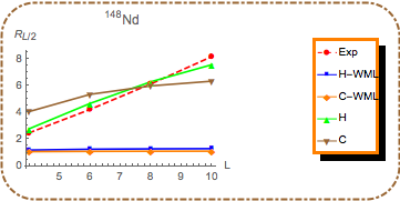
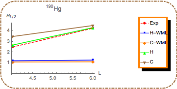
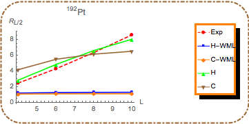
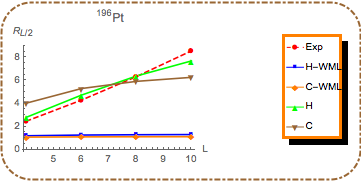
Figure 1: The energy ratios in the absence of ML and in its presence

experimental data by

$$\sigma=\sqrt{\frac{{\sum^{m}_{i=1}(E_{i}(exp))-E_{i}(th))^{2}}}{(m-1)E(2^{+}_{1})^{2}}}$$ (22)

where $m$ is the number of states, while $E_{i}(exp)$ and $E_{i}(th)$ represent the theoretical and experimental energies of the $i^{th}$ level, respectively. $E(2^{+}_{1})$ is the energy of the first excited level of the ground state band.

From the Eq (9) and (8), one can see that both potentials have mathematically similar behaviors. If we give the same value to the parameter $c$ in Coulomb potential (Eq.(8)) and $\delta$ in the Hulthén one (Eq.(9)), we get overcome curves. The Figure (1) shows that in the absence of minimal length case, the obtained results for energy ratios with both potentials are identical for all even-even nuclei, while in its presence, the calculated energy ratios $R_{L/2}$ with Hulthén potential are

Table 1: The comparison of the obtained results by the two equations: (12) and (14), for the ground state band $(n=0)$ and the $\beta$ band $(n=1)$ with the experimental data [14]. The values of free parameters is also shown

Nucleus	${R_{0,4}}$	${R_{0,6}}$	${R_{0,8}}$	${R_{0,10}}$	${R_{1,0}}$	${R_{1,2}}$	${R_{1,4}}$	${R_{1,6}}$	$\alpha$	$\delta$	$c$	$\sigma$
104Ru Exp	2.48	4.35	6.48	8.69	2.76	4.23	5.81
H	2.82	4.78	6.49	7.85	3.91	4.51	5.62		0.00003	0.003		0.63
C	4.121	5.42	6.06	6.42	4.11	4.63	5.51		0.58		-1.31	1.36
120Xe Exp	2.44	4.23	6.34	8.77	2.82	3.95	5.31
H	2.81	4.75	6.43	7.76	3.89	4.48	5.58		0.00003	0.003		0.70
C	4.07	5.35	5.98	6.33	4.06	4.58	5.44		0.58		-1.31	1.43
122Xe Exp	2.50	4.43	6.69	9.18	3.47	4.51
H	2.86	4.94	6.81	8.34	4.18	4.79			0.00004	0.003		0.58
C	4.29	5.67	6.35	6.72	4.29	4.84			0.58		-1.31	1.53
124Xe Exp	2.48	4.37	6.58	8.96	3.58	4.60	5.69
H	2.85	4.89	6.71	8.19	4.10	4.70	5.86		0.00003	0.003		0.47
C	4.25	5.61	6.28	6.65	4.25	4.79	5.71		0.58		-1.31	1.32
148Nd Exp	2.49	4.24	6.15	8.19	3.04	3.88	5.32	7.12
H	2.79	4.68	6.30	7.58	3.77	4.36	5.44	6.63	0.00003	0.003		0.49
C	4.07	5.36	5.99	6.34	4.07	4.58	5.45	6.00	0.58		-1.31	1.31
150Sm Exp	2.32	3.83	5.50	7.29	2.22	3.13	4.34	6.31
H	2.66	4.27	5.54	6.47	3.23	3.78	4.73	5.70	0.00003	0.004		0.64
C	3.58	4.66	5.19	5.48	3.55	4.00	4.73	5.19	0.58		-1.30	1.17
152Gd Exp	2.19	3.57	5.07	6.68	1.79	2.70	3.72	4.85
H	2.53	3.88	4.86	5.54	2.80	3.31	4.15	4.93	0.00003	0.005		0.67
C	3.17	4.08	4.52	4.77	3.12	3.52	4.14	4.53	0.41		-1.52	1.06
172Os Exp	2.66	4.63	6.70	8.89	3.33	3.56	5.00	6.81
H	2.81	4.76	6.45	7.79	3.88	4.47	5.58	6.82	0.00003	0.003		0.63
C	4.19	5.52	6.17	6.54	4.18	4.72	5.61	6.18	0.58		-1.31	1.29
190Hg Exp	2.50	4.26			3.07	3.77	4.74	6.03
H	2.68	4.31			3.44	3.88	4.58	5.02	0.00004	0.004		0.16
C	3.48	4.51			3.48	4.51	5.01	5.30	0.95		-1.02	0.66
192Pt Exp	2.48	4.31	6.38	8.62	3.78	4.55
H	2.84	4.85	6.629	8.06	4.02	4.63			0.00003	0.003		0.41
C	4.18	5.50	6.16	6.52	4.17	4.71			0.58		-1.31	1.33
196Pt Exp	2.47	4.29	6.33	8.56	3.19	3.83
H	2.80	4.72	6.37	7.68	3.82	4.41			0.00002	0.003		0.60
C	4.03	5.29	5.91	6.26	4.02	4.53			0.58		-1.31	1.41

Table 2: The comparison of the present model with experimental data, for theoretical predictions calculated with the two potentials: Hulthén and Coulomb, for $B(E2)$ transition rates [15]

Nucleus	$\frac{4_{1}\rightarrow 2_{1}}{2_{1}\rightarrow 0_{1}}$	$\frac{6_{1}\rightarrow 4_{1}}{2_{1}\rightarrow 0_{1}}$	$\frac{8_{1}\rightarrow 6_{1}}{2_{1}\rightarrow 0_{1}}$	$\frac{10_{1}\rightarrow 8_{1}}{2_{1}\rightarrow 0_{1}}$	$\frac{0_{\beta}\rightarrow 2_{1}}{2_{1}\rightarrow 0_{1}}$	$\frac{2_{\beta}\rightarrow 2_{1}}{2_{1}\rightarrow 0_{1}}$	$\frac{2_{\beta}\rightarrow 4_{1}}{2_{1}\rightarrow 0_{1}}$	$\frac{2_{\beta}\rightarrow 0_{\beta}}{2_{1}\rightarrow 0_{1}}$		$\sigma$
100Mo  Exp	1.86(11)	2.54(38)	3.32(49)		2.49(12)	0	0.97(49)	0.38(11)
H	1.88	3.33	6.16	11.26	1.52	0.14	2.29	2.98		0.84
C	2.25	1.41	0.76	0.43	1.41	4.88	0.73	0.07		1.06
108Ru Exp	1.65(20)
H	1.59	2.13	2.88	3.98	0.56	0.08	0.58	2.04		0.05
C	2.61	1.71	0.93	0.53	1.98	5.82	0.77	0.04		0.96
128Xe  Exp	1.47(15)	1.94(20)	2.39(30)
H	1.73	2.65	4.22	6.83	0.97	0.11	1.25	2.52		0.48
C	2.44	1.57	0.85	0.48	1.71	5.39	0.75	0.05		0.83
146Nd  Exp	1.47(39)
H	1.80	2.97	5.11	8.84	1.23	0.13	1.73	2.76		0.33
C	2.35	1.50	0.81	0.45	1.57	5.15	0.74	0.06		0.88
148Nd  Exp	1.62	1.76	1.69		0.54	0.25	0.28
H	1.71	2.57	3.99	6.33	0.90	0.11	1.14	2.45		0.59
C	2.49	1.61	0.87	0.49	1.78	5.50	0.76	0.05		0.91
150Sm Exp	1.93(30)	2.63(88)	2.98(158)		0.93(9)			1.93
H	1.78	2.86	4.81	8.15	1.14	0.12	1.56	2.68		0.57
C	2.40	1.53	0.83	0.47	1.64	5.26	0.74	0.05		0.76
172Os  Exp	1.56(6)	1.82(10)	1.99(11)	2.29(26)	0.33(5)	0.04	0.12(1)	0.62(6)
H	1.70	2.52	3.87	6.06	0.87	0.11	1.07	2.42		1.01
C	2.50	1.62	0.88	0.50	1.81	5.54	0.76	0.05		1.16
190Hg  Exp
H	1.77	2.83	4.73	7.97	1.12	0.12	1.52	2.66
C	2.37	1.51	0.82	0.46	1.60	5.20	0.74	0.062
192Pt Exp	1.56	1.22
H	1.68	2.46	3.72	5.75	0.82	0.10	1.00	2.37		0.48
C	2.50	1.62	0.88	0.49	1.80	5.54	0.76	0.050		0.09
196Pt Exp	1.48(2)	1.80(10)	1.92(25)				=0	0.12
H	1.70	2.54	3.93	6.19	0.89	0.11	1.10	2.43		0.60
C	2.48	1.60	0.87	0.49	1.77	5.48	0.759	0.05		0.63

fairly better than those obtained with Coulomb one. The best candidate nuclei for the model with Hulthén potential are: ¹⁷²Os, ¹⁹²Pt, ¹⁹⁶Pt and ¹⁹⁰Hg.

7 Conclusion

In this work, we have solved the Bohr-Mottelson Hamiltonian in the $\gamma$-rigid regime within the minimal length formalism with two well-known potentials: Coulomb and Hulthén.

From the comparison between the energy spectra and transition probabilities in the two cases: presence and absence of the minimal length, one can conclude that the obtained results with Hulthén potential within the ML are better. This latter reproduces well the $X(3)$ candidates which already have been obtained including the predicted new one: ¹⁹⁰Hg.

References

- [1] F. Iachello, Phys. Rev. Lett. 85 (17) (2000) 3580.
- [2] F. Iachello, Phys. Rev. Lett. 87 (5) (2001) 052502.
- [3] D. Bonatsos, D. Lenis, D. Petrellis, P. A. Terziev, I. Yigitoglu, Phys. Lett. B632 (2006) 238–242.
- [4] M. Chabab, A. El Batoul, A. Lahbas, M. Oulne, Phys. Lett.B B758 (2016) 212–218.
- [5] D. Bonatsos, D. Lenis, D. Petrellis, P. A. Terziev, I. Yigitoglu, Phys. Lett. B621 (2005) 102–108.
- [6] M. J. Ermamatov, P. R. Fraser, Phys. Rev. C84 (2011) 044321.
- [7] R. Budaca, P. Buganu, M. Chabab, A. Lahbas, M. Oulne, Annals Phys. 375 (2016) 65–90.
- [8] H. Ciftci, R. L. Hall, N. Saad, J. Phys. A: Math. Gen. 36 (47) (2003) 11807.
- [9] I. Boztosun, M. Karakoc, Chin. Phys. Lett. 24 (11) (2007) 3028.
- [10] M. Chabab, A. El Batoul, A. Lahbas, M. Oulne, Annals Phys. 392 (2018) 142–156.
- [11] M. Chabab, A. El Batoul, M. Oulne, Z. Naturforsch. A 71 (1) (2016) 59–68.
- [12] I. S. Gradshteyn, I. M. Ryzhik, Table of Integral, Series, and Products, Academic, New York, 1980.
- [13] L. Wilets, M. Jean, Phys. Rev. 102 (3) (1956) 788.
- [14] Brookhaven national laboratory, national nuclear data center, http://www.nndc.bnl.gov/nndc/ensdf/.
- [15] D. Bonatsos, P. E. Georgoudis, N. Minkov, D. Petrellis, C. Quesne, Phys. Rev. C88 (3) (2013) 034316.