Towards the renormalization group flow of Hořava gravity
in $(3+1)$ dimensions

Abstract

We compute the renormalization group running of the Newton constant and the parameter $\lambda$ in $(3+1)$-dimensional projectable Hořava gravity. We use the background field method expanding around configurations with flat spatial metric, but non-vanishing shift. This allows us to reduce the number of interaction vertices and thereby drastically simplify the calculations. The gauge invariant $\beta$-function of $\lambda$ has two families of zeros, attractive in the infrared and ultraviolet respectively. They are candidates for the fixed points of the full renormalization group flow of the theory, once the $\beta$-functions for the rest of the couplings are added.

I Introduction

Since the formulation of general relativity (GR) a century ago and of quantum mechanics a few years later the quest for a theory unifying the two — quantum gravity (QG) — has been one of the biggest endeavors in theoretical physics. While other known fundamental interactions are successfully described within the formalism of local perturbative quantum field theory (QFT), most approaches to QG involve departures from this framework. Despite a number of impressive achievement of these research programs, the quest for QG remains largely unaccomplished. Thus, it is reasonable to wonder if there is still a way to formulate QG within the realm of QFT.

However, a straightforward approach to this goal fails due to the dimensionful character of Newton’s constant $G$ in dimensions greater than two, in particular in $(3+1)$ dimensions. This renders the theory non-renormalizable, with the number of divergences increasing at every loop order and requiring an infinite set of counterterms suppressed by higher powers of the Planck mass $M_{P}\sim\sqrt{G^{-1}}\sim 10^{19}{\rm GeV}$. Thus, perturbative GR can be thought at most as an effective low-energy theory of gravitational interactions, see e.g. Donoghue (1994); Burgess (2004); Donoghue et al. (2017), unable to describe physics above the ultraviolet (UV) cutoff given by $M_{P}$.

A simple way out of this problem in four space-time dimensions is to extend the gravitational Lagrangian with terms quadratic in curvature Stelle (1977); Fradkin and Tseytlin (1981); Avramidi and Barvinsky (1985) so that UV divergences are softened by higher powers of four-momenta in the propagators. Although this theory is thereby renormalizable and even asymptotically free for some regions of the parameter space, unitarity is jeopardized by the presence of four time derivatives in the action, which gives rise to a propagating Ostrogradsky ghost with negative norm in the Hilbert space Stelle (1978); Woodard (2015).

It was pointed out by P. Hořava Hořava (2009) that unitarity can be preserved in this kind of models if we sacrifice Lorentz invariance (LI) at very high energies. This allows one to introduce into the Lagrangian extra higher spatial derivatives which will soften UV divergences while at the same time keeping only two time derivatives, so that the ghosts are avoided. For this proposal to work, one must supplement the spacetime manifold with a preferred foliation into spatial slices and a privileged time direction. Then it is possible to formulate a theory containing only marginal operators and relevant deformations with respect to an anisotropic (Lifshitz) scaling in $(d+1)$ dimensions,

$$t\rightarrow b^{-d}t,\qquad x^{i}\rightarrow b^{-1}x^{i}\;,$$ (1)

instead of the usual isotropic scaling. As a consequence, a theory of gravity formulated under this setting cannot be LI nor completely diffeomorphism invariant. Instead, it will enjoy a restricted symmetry in terms of foliation preserving diffeomorphisms (FDiff),

$$t\rightarrow t^{\prime}(t),\qquad x^{i}\rightarrow x^{\prime i}(t,x)\;,$$ (2)

where $t^{\prime}(t)$ must be a monotonic function. That is, we are left with invariance under time reparameterizations and spatial time-dependent diffeomorphisms.

Hořava’s proposal gave rise to numerous follow-up publications studying different aspects of Hořava gravity (HG) (see Mukohyama (2010); Sotiriou (2011); Blas (2018); Wang (2017) for reviews). These include an exhaustive study of the low energy regime of the theory, which led to the identification of a version of HG – the healthy non-projectable model Blas et al. (2010) – which can reproduce the known phenomenology of GR at the scales in which the latter has been tested Blas and Lim (2015). While its parameter space has been strongly constrained by the observation of a gravitational wave signal from a binary neutron star merger Abbott et al. (2017), it still remains phenomenologically viable Emir Gümrükçüoğlu et al. (2018). In this theory, a certain amount of LI violation persists at all scales Blas et al. (2011). This can lead to interesting cosmological applications Blas and Sibiryakov (2011a); Audren et al. (2013). However, it also demands the presence of a mechanism suppressing the percolation of LI violation to the visible matter sector, where LI has been tested to a very high precision Liberati (2013).

Regarding renormalizability, the situation is less clear. Although the Lagrangian of the non-projectable model is power-counting renormalizable, the lapse element of the metric induces an instantaneous interaction Blas et al. (2011); Blas and Sibiryakov (2011b) which can potentially lead to non-local loop divergences Barvinsky et al. (2016). Whether this indeed happens or not is an open question.

There has been a significant progress in understanding the quantum dynamics of a reduced version of HG known as the projectable model, where the lapse $N$ is restricted to be only time-dependent. Then it can be algebraically fixed to take a given value, say $N=1$. In this way one gets rid of time reparameterization invariance as a symmetry of the theory, being left only with spatial diffeomorphisms. This version of the theory does not have a stable homogeneous vacuum with flat Minkowski metric and thus is unlikely to reproduce realistic phenomenology, at least in the controllable regime of weak coupling Blas et al. (2009); Koyama and Arroja (2010); Blas et al. (2011) (see, however, Mukohyama (2010); Izumi and Mukohyama (2011); Gumrukcuoglu et al. (2012)). Nevertheless, it captures several salient features of QG, such as propagating spin-2 gravitons (in spacetime dimensions greater than 3) and a large gauge group of coordinate transformations precluding existence of local gauge-invariant observables. The projectable model has been proven to be renormalizable in the strict sense, i.e. all divergences are proportional to gauge invariant operators already present in the bare action, in any space-time dimension Barvinsky et al. (2016, 2018).

Furthermore, the computation of the full renormalization group (RG) flow of the theory in $(2+1)$ spacetime dimensions reveals the presence of an asymptotically free UV fixed point Barvinsky et al. (2017a). Unlike $(2+1)$-dimensional GR, this theory possesses a propagating scalar degree of freedom and thus provides an example of a perturbatively UV complete gravitational field theory with non-trivial local dynamics. Other results along these lines include the study of a conformal reduction of the $(2+1)$-dimensional theory Benedetti and Guarnieri (2014), the computation of the anomalous dimension of the cosmological constant Griffin et al. (2017), also in $(2+1)$ dimensions, and the contribution of scalar matter into the renormalization of the gravitational couplings D’Odorico et al. (2014).

In this paper we make a step towards uncovering the RG flow of HG in $(3+1)$ dimensions. This case differs from the $(2+1)$-dimensional model in two respects. First, the physical spectrum of the theory now includes a spin-2 mode — graviton. Second, on the technical side, the structure of the propagators and vertices is significantly more complicated than in $(2+1)$-dimensional HG, which makes a direct application of the approach used in Barvinsky et al. (2017a) infeasible. We find a way to modify this approach that allows us to compute the 1-loop $\beta$-functions of the two couplings entering the kinetic part of the action. Renormalization of the potential part requires different techniques and will be reported elsewhere.

The paper is organized as follows. In Sec. II we review the structure of projectable HG and its relevant properties. In Sec. III we describe our calculation. In Sec. IV we report the results for the $\beta$-functions and discuss their implications. Section V is devoted to conclusions. Appendices provide additional details.

II Projectable Hořava Gravity

Hořava gravity Hořava (2009) is formulated by considering the spacetime metric together with a preferred foliation along the time direction. This induces an Arnowitt–Deser–Misner (ADM) decomposition of the metric,

$$ds^{2}=N^{2}\mathrm{d}t^{2}-\gamma_{ij}(\mathrm{d}x^{i}+N^{i}\mathrm{d}t)(\mathrm{d}x^{j}+N^{j}\mathrm{d}t)\;.$$ (3)

The lapse $N$, the shift $N^{i}$ and the spatial metric $\gamma_{ij}$ on the foliation slices transform in the standard way under FDiff transformations,

$$N\mapsto N\frac{\mathrm{d}t}{\mathrm{d}t^{\prime}},\qquad N^{i}\mapsto\left(N^{j}\frac{\partial x^{\prime i}}{\partial x^{j}}-\frac{\partial x^{\prime i}}{\partial t}\right)\frac{\mathrm{d}t}{\mathrm{d}t^{\prime}},\qquad\gamma_{ij}\mapsto\gamma_{kl}\frac{\partial x^{k}}{\partial x^{\prime i}}\frac{\partial x^{l}}{\partial x^{\prime j}}\;.$$ (4)

Their dimensions under the anisotropic scaling (1) are,

$$[N]=[\gamma_{ij}]=0,\qquad[N^{i}]=d-1\;.$$ (5)

The FDiff symmetry, together with time-reversal invariance, parity and the requirement of power-counting renormalizability fix the action of HG to be

$$S=\frac{1}{2G}\int\mathrm{d}t\mathrm{d}^{d}x\sqrt{\gamma}\,N\left(K_{ij}K^{ij}-\lambda K^{2}-{\cal V}\right)\;.$$ (6)

Here $G$ and $\lambda$ are dimensionless coupling constants and the extrinsic curvature of the foliation is given by

$$K_{ij}=\frac{1}{2N}\left(\dot{\gamma}_{ij}-\nabla_{i}N_{j}-\nabla_{j}N_{i}\right)\;,$$ (7)

where dot denotes time derivative and $\nabla_{i}$ is the covariant derivative associated to the spatial metric; $K\equiv K_{ij}\gamma^{ij}$ denotes the trace of $K_{ij}$. FDiff transformations (4) are compatible with an assumption of the lapse function being constant on the foliation slices, $N=N(t)$. This specifies the projectable version of the model Hořava (2009), to which we restrict in what follows. In this case, we can set $N=1$ as an algebraic gauge fixing for time reparameterization invariance, eliminating it from the set of dynamical fields and leaving us only with spatial diffeomorphisms as a gauge symmetry.

The potential ${\cal V}$ contains all possible marginal and relevant operators invariant under FDiff and without time derivatives. In $d=3$ and after using Bianchi identities and integration by parts, these reduce to Sotiriou et al. (2009),

$${\cal V} =2\Lambda-\eta R+\mu_{1}R^{2}+\mu_{2}R_{ij}R^{ij}$$

$$+\nu_{1}R^{3}+\nu_{2}RR_{ij}R^{ij}+\nu_{3}R^{i}_{j}R^{j}_{k}R^{k}_{i}+\nu_{4}\nabla_{i}R\nabla^{i}R+\nu_{5}\nabla_{i}R_{jk}\nabla^{i}R^{jk}\;,$$ (8)

where $R_{ij}$ is the Ricci tensor corresponding to the spatial metric and we have used the fact that in three dimensions the Riemann tensor is expressed in terms of $R_{ij}$.

The spectrum of perturbations propagated by this action contains a transverse-traceless (tt) graviton and an additional scalar mode Blas et al. (2009); Barvinsky et al. (2016). Both modes have positive-definite kinetic terms as long as $G>0$ and $\lambda\in\left(-\infty,\frac{1}{3}\right)\cup(1,\infty)$ and the theory admits unitary quantization. Their dispersion relations around a flat background are

$$\omega^{2}_{tt}=\eta k^{2}+\mu_{2}k^{4}+\nu_{5}k^{6}\;,$$ (9a)

$$\omega^{2}_{s}=\frac{1-\lambda}{1-3\lambda}\big{(}-\eta k^{2}+(8\mu_{1}+3\mu_{2})k^{4}\big{)}+\nu_{s}k^{6}\;,$$ (9b)

where $k$ is the spatial momentum and we have defined

$$\nu_{s}=\frac{(1-\lambda)(8\nu_{4}+3\nu_{5})}{1-3\lambda}\;.$$ (10)

A problem arises in the low-energy limit, where the dispersions relations are dominated by the terms proportional to $k^{2}$. Due to the negative sign in front of this term, the scalar mode behaves as a tachyon at low energies, implying that flat space is not a stable vacuum of the theory. Attempts to suppress the instability by choosing $\lambda$ close to 1 lead to the loss of perturbative control Blas et al. (2009); Koyama and Arroja (2010); Blas et al. (2011) (see, however, Mukohyama (2010); Izumi and Mukohyama (2011); Gumrukcuoglu et al. (2012) for suggestions to restore the control by rearranging the perturbation theory at the classical level). Alternatively, the instability can be eliminated by tuning $\eta=0$ or by expanding around a curved vacuum. In both cases the theory does not appear to reproduce GR in the low-energy limit, as there is no regime where the dispersion relation of the tt-graviton would have the relativistic form $\omega^{2}_{tt}\propto k^{2}$. On the other hand, both dispersion relations (9) are perfectly regular at high momenta for $\nu_{5},\nu_{s}>0$. This is the relevant region for the structure of UV divergences which are the focus of the present paper.

For the rest of this work we restrict to the sector of marginal operators that dominate the UV behavior of the theory by setting $\eta=\mu_{1}=\mu_{2}=0$. We also perform a Wick rotation to “Euclidean” time $\tau$, which amounts to flipping the sign of the potential term. Thus we consider the action,

$$S=\frac{1}{2G}\int\mathrm{d}\tau\mathrm{d}^{3}x\sqrt{\gamma}\, \left(K_{ij}K^{ij}-\lambda K^{2}+\nu_{1}R^{3}+\nu_{2}RR_{ij}R^{ij}\right.$$

$$\left.+\nu_{3}R^{i}_{j}R^{j}_{k}R^{k}_{i}+\nu_{4}\nabla_{i}R\nabla^{i}R+\nu_{5}\nabla_{i}R_{jk}\nabla^{i}R^{jk}\right)\;.$$ (11)

We are interested in the 1-loop correction to this action and the corresponding RG flow of the couplings $\{G,\lambda,\nu_{1},\ldots,\nu_{5}\}$.

III The background-field approach

In our calculation we use the background field method Abbott (1982). We expand the fields about arbitrary background values,

$$\gamma_{ij}=\bar{\gamma}_{ij}+h_{ij},\qquad N_{i}=\bar{N}_{i}+n_{i}\;,$$ (12)

and expand the action (II) up to second order in the fluctuations $h_{ij},n_{i}$. One-loop divergences will be captured as contributions to operators carrying background fields after integrating out the fluctuations. This procedure should work in general and, similarly to the case in $(2+1)$ dimensions, we should be able to obtain the contributions to the whole set of coupling constants $\{G,\lambda,\nu_{a}\}$ by an appropriate choice of background. However, the complexity of computations quickly grows with the number of space-time dimensions. This stems mainly from the increased number of terms in the potential part of the action and their more complicated structure. Indeed, in $(2+1)$ dimensions there is a single term $R^{2}$ which generates about twenty different contributions when expanded about an arbitrary background (12). In $(3+1)$ dimensions we have five operators shown in (II) which generate hundreds of structures. This makes a complete calculation of the RG flow in any dimension higher than $(2+1)$ highly challenging. In particular, it does not appear feasible to apply the diagrammatic approach of Barvinsky et al. (2017a) to renormalization of the operators in the potential. Rather, one will have to use the covariant techniques developed in Barvinsky and Vilkovisky (1985); D’Odorico et al. (2015); Barvinsky et al. (2017b) or other advanced tools.

Fortunately, the situation is different for the operators in the kinetic part of the action, i.e. the two operators involving the extrinsic curvature. We observe that the latter contains the shift vector $N^{i}$ in a specific combination. Then, exploiting the known gauge invariance of divergences Barvinsky et al. (2016, 2018), we can extract the renormalization of $G$ and $\lambda$ not only from the terms with time derivatives of the spatial metric as in Barvinsky et al. (2017a), but also from terms with spatial gradients of $N^{i}$. Since the shift only enters into the kinetic term, all interaction vertices contributing to the renormalization of these operators will also come exclusively from the expansion of the kinetic term. The potential, as we will see shortly, only contributes into the propagators. Furthermore, we can restrict to backgrounds with flat spatial metric $\bar{\gamma}_{ij}=\delta_{ij}$, as long as we allow the background shift $\bar{N}^{i}$ to take arbitrary space-dependent values. All this together means that we can derive the renormalization of $G$ and $\lambda$ avoiding the complexity mentioned above and allows us to carry out the computation in a reasonably simple way.

According to the above discussion, we consider a family of backgrounds characterized by flat spatial metric and an arbitrary space-dependent shift. Thus, we specify (12) to

$$\gamma_{ij}=\delta_{ij}+h_{ij}(\tau,x),\qquad N_{i}=\bar{N}_{i}(x)+n_{i}(\tau,x)\;.$$ (13)

The Lagrangian is then expanded to quadratic order in $h_{ij}$ and $n_{i}$. Note that we define the perturbation of the shift with lower indices: this choice turns out to be more convenient as it reduces the number of terms in the perturbed Lagrangian. The perturbation of the component with the upper indices is then given by

$$\delta N^{i}=n^{i}-h^{i}_{j}\bar{N}^{j}\;,$$ (14)

where on the r.h.s. the indices are raised using the flat background metric $\delta^{ij}$. From now on we will not distinguish upper and lower indices in the expressions expanded around the background (13); all repeated spatial indices will be simply summed over.

We are interested in those operators in the effective action for the background fields that contain the background shift. With our choice of flat background spatial metric, these are

$$S_{\bar{N}}=\frac{1}{2G}\int\mathrm{d}\tau\mathrm{d}^{3}x\,\left(\frac{1}{2}\partial_{i}\bar{N}_{j}\partial_{i}\bar{N}_{j}+\left(\frac{1}{2}-\lambda\right)\partial_{i}\bar{N}_{i}\partial_{j}\bar{N}_{j}\right)\;.$$ (15)

By computing the one-loop contribution to these operators we will be able to capture the renormalization of $G$ and $\lambda$.

III.1 Covariant gauge fixing

The action (II) is invariant under the residual part of FDiff that preserves the condition $N=1$, namely time-dependent spatial diffeomorphism of the form

$$x^{i}\rightarrow x^{\prime i}(\tau,x)\;.$$ (16)

In order to proceed with the quantization of the theory we must thus append the bare action with a gauge fixing term for this symmetry. Within the background-field approach, the latter is chosen to be invariant under the background gauge transformations that in our case read,

$$\bar{N}^{i}\mapsto\bar{N}^{j}\frac{\partial x^{\prime i}}{\partial x^{j}}-\frac{\partial x^{\prime i}}{\partial\tau},\qquad\bar{\gamma}_{ij}\mapsto\bar{\gamma}_{kl}\frac{\partial x^{k}}{\partial x^{\prime i}}\frac{\partial x^{l}}{\partial x^{\prime j}}\;.$$ (17)

This ensures that the one-loop background effective action consists of gauge invariant operators and allows one to extract the renormalized couplings as the coefficients in front of such operators Abbott (1982). By comparing (17) to (4) it is straightforward to see that the shift perturbation with upper index $\delta N^{i}\equiv N^{i}-\bar{N}^{i}$ and the metric perturbation $h_{ij}$ transform as a contravariant vector and a covariant tensor respectively. They serve as the building blocks to construct the gauge fixing term.

We choose the gauge fixing introduced in Barvinsky et al. (2016) which ensures that the propagators of all fluctuations decay uniformly in frequency and momentum in a way compatible with the anisotropic scaling. It reads,

$$S_{\rm gf}=\frac{\sigma}{2G}\int\mathrm{d}\tau\mathrm{d}^{3}x\,F^{i}{\cal O}_{ij}F^{j}\;,$$ (18)

where

$$F^{i}=D_{\tau}(\delta N^{i})+\varsigma\bar{K}^{i}_{j}\,\delta N^{j}+\frac{1}{2\sigma}\left({\cal O}^{-1}\right)^{ij}\left(\partial_{k}h^{k}_{j}-\lambda\partial_{j}h\right)\;,$$ (19a)

$$\left({\cal O}^{-1}\right)^{ij}=\delta^{ij}\Delta^{2}+\xi\partial^{i}\Delta\partial^{j}\;.$$ (19b)

Here $h\equiv h_{i}^{i}$ is the trace of the metric fluctuations, $\Delta\equiv\partial_{i}\partial^{i}$ is the flat-space Laplacian, $\sigma$ and $\xi$ are free parameters and

$$D_{\tau}(\delta N^{i})=\delta\dot{N}^{i}-\bar{N}^{k}\,\partial_{k}\delta N^{i}+\partial_{k}\bar{N}^{i}\,\delta N^{k}\;$$ (20)

is the covariant time-derivative of $\delta N^{i}$. Note that we have added to the gauge-fixing function a contribution proportional to the background extrinsic curvature $\bar{K}^{i}_{j}$ with an arbitrary coefficient $\varsigma$. This additional freedom, which was not present in the original gauge fixing of Barvinsky et al. (2016), can be used to simplify the Lagrangian for perturbations and as an extra check of gauge invariance of our results.

The presence of the non-local operator ${\cal O}_{ij}$ leads to appearance of non-local terms in the gauge-fixing action that are quadratic in $\delta N^{i}$. Following Barvinsky et al. (2016, 2017a) we eliminate this non-locality by integrating in an extra field $\pi_{i}$, so that we rewrite,

$$\begin{split}&\frac{\sigma}{2G}\big{(}D_{\tau}(\delta N^{i})+\varsigma\bar{K}^{i}_{j}\,\delta N^{j}\big{)}\,{\cal O}_{ik}\,\big{(}D_{\tau}(\delta N^{k})+\varsigma\bar{K}^{k}_{l}\delta N^{l}\big{)}\\ &\mapsto\frac{1}{2G}\left[\frac{1}{\sigma}\pi_{i}\left({\cal O}^{-1}\right)^{ij}\pi_{j}-2i\pi_{i}\big{(}D_{\tau}(\delta N^{i})+\varsigma\bar{K}^{i}_{j}\delta N^{j}\big{)}\right]\;.\end{split}$$ (21)

Then the whole gauge-fixing action takes the local form,

$$\begin{split}S_{\rm gf}=&\frac{1}{2G}\int\mathrm{d}\tau\mathrm{d}^{3}x\,\left[\frac{1}{\sigma}\pi_{i}\left({\cal O}^{-1}\right)^{ij}\pi_{j}-2i\pi_{i}\big{(}D_{\tau}(\delta N^{i})+\varsigma\bar{K}^{i}_{j}\,\delta N^{j}\big{)}\right.\\ &\left.+\big{(}D_{\tau}(\delta N^{i})+\varsigma\bar{K}^{i}_{j}\,\delta N^{j}\big{)}\big{(}\partial_{k}h^{k}_{i}-\lambda\partial_{i}h\big{)}+\frac{1}{4\sigma}\big{(}\partial_{k}h^{k}_{i}-\lambda\partial_{i}h\big{)}\left({\cal O}^{-1}\right)^{ij}\big{(}\partial_{l}h^{l}_{j}-\lambda\partial_{j}h\big{)}\right].\end{split}$$ (22)

Finally, we have to add the anticommuting Faddeev-Popov ghost $c^{i}$ and antighost $\bar{c}_{i}$. The action for them is constructed out of the gauge fixing function as

$$S_{\rm gh}=-\frac{1}{G}\int\mathrm{d}\tau\mathrm{d}^{3}x\,\bar{c}_{i}\mathbf{s}F^{i}\;,$$ (23)

where the BRST operator $\mathbf{s}$ can be understood as implementing a gauge transformation with the gauge parameter replaced by the ghost,

$$\mathbf{s}h_{ij}=\partial_{i}c_{j}+\partial_{j}c_{i}+\partial_{i}c^{k}h_{jk}+\partial_{j}c^{k}h_{ik}+c^{k}\partial_{k}h_{ij}\;,$$ (24a)

$$\mathbf{s}(\delta N^{i})=D_{\tau}c^{i}-\delta N^{j}\partial_{j}c^{i}+c^{j}\partial_{j}\delta N^{i}\;.$$ (24b)

To sum up, the total action that we are going to work with reads,

$$S_{\rm tot}=S^{(2)}+S_{\rm gf}+S_{\rm gh}\;,$$ (25)

where $S^{(2)}$ is the result of expanding (II) to quadratic order in $h_{ij},n_{i}$ and $S_{\rm gf}$, $S_{\rm gh}$ are given by (22), (23) respectively.

III.2 Propagators

To set up the computation along the lines of Barvinsky et al. (2017a), we need to derive the propagators for the dynamical field $\{h_{ij},n_{i},\pi_{j},c_{i},\bar{c}_{j}\}$. They are obtained by setting the background shift $\bar{N}_{i}$ to zero in the total quadratic action for the fluctuations (25). The resulting Lagrangian splits into several pieces,

$${\cal L}_{h}=\frac{1}{2G}\bigg{[} \frac{1}{4}\dot{h}_{ij}^{2}-\frac{\lambda}{4}\dot{h}^{2}-\frac{\nu_{5}}{4}h_{ij}\Delta^{3}h_{ij}+\bigg{(}-\frac{\nu_{5}}{2}+\frac{1}{4\sigma}\bigg{)}\partial_{k}h_{ki}\,\Delta^{2}\partial_{l}h_{li}$$

$$+\bigg{(}-\nu_{4}-\frac{\nu_{5}}{2}-\frac{\xi}{4\sigma}\bigg{)}\partial_{i}\partial_{k}h_{ik}\,\Delta\partial_{j}\partial_{l}h_{jl}+\bigg{(}2\nu_{4}+\frac{\nu_{5}}{2}+\frac{\lambda(1+\xi)}{2\sigma}\bigg{)}\Delta^{2}h\,\partial_{i}\partial_{k}h_{ik}$$

$$+\bigg{(}-\nu_{4}-\frac{\nu_{5}}{4}-\frac{\lambda^{2}(1+\xi)}{4\sigma}\bigg{)}h\Delta^{3}h\bigg{]},$$ (26a)

$${\cal L}_{n}=\frac{1}{2G}\bigg{[} \frac{1}{\sigma}\pi_{i}\Delta^{2}\pi_{i}-\frac{\xi}{\sigma}\partial_{i}\pi_{i}\,\Delta\partial_{j}\pi_{j}-2i\pi_{i}\dot{n}_{i}-\frac{1}{2}n_{i}\Delta n_{i}+\bigg{(}\frac{1}{2}-\lambda\bigg{)}(\partial_{i}n_{i})^{2}\bigg{]},$$ (26b)

$${\cal L}_{\bar{c}}=-\frac{1}{G}\bigg{[} \bar{c}_{i}\ddot{c}_{i}+\frac{1}{2\sigma}\bar{c}_{i}\Delta^{3}c_{i}-\frac{1+2\xi-2\lambda(1+\xi)}{2\sigma}\partial_{i}\bar{c}_{i}\,\Delta^{2}\partial_{k}c_{k}\bigg{]}.$$ (26c)

In deriving these expressions we used integration by parts. Note that our choice of the gauge fixing ensures cancellation of the terms mixing $h_{ij}$ and $n_{i}$ in the expansion of the bare Lagrangian Barvinsky et al. (2016). Inversion of the differential operators appearing in (26) yields the propagators,

$$\langle h_{ij}h_{kl}\rangle=G\bigg{[}2(\delta_{ik}\delta_{jl}+\delta_{il}\delta_{jk}){\cal P}_{tt}-2\delta_{ij}\delta_{kl}\bigg{(}{\cal P}_{tt}-\frac{1-\lambda}{1-3\lambda}{\cal P}_{s}\bigg{)}$$

$$\qquad\qquad-2(\delta_{ik}\hat{k}_{j}\hat{k}_{l}+\delta_{il}\hat{k}_{j}\hat{k}_{k}+\delta_{jk}\hat{k}_{i}\hat{k}_{l}+\delta_{jl}\hat{k}_{i}\hat{k}_{k})({\cal P}_{tt}-{\cal P}_{1})+2(\delta_{ij}\hat{k}_{k}\hat{k}_{l}+\hat{k}_{i}\hat{k}_{j}\delta_{kl})({\cal P}_{tt}-{\cal P}_{s})$$

$$\qquad\qquad+2\hat{k}_{i}\hat{k}_{j}\hat{k}_{k}\hat{k}_{l}\bigg{(}{\cal P}_{tt}+\frac{1-3\lambda}{1-\lambda}{\cal P}_{s}-4{\cal P}_{1}+\frac{2}{1-\lambda}{\cal P}_{2}\bigg{)}\bigg{]}\;,$$ (27a)

$$\langle n_{i}n_{j}\rangle=G\bigg{[}\frac{k^{2}}{\sigma}(k^{2}\delta_{ij}-k_{i}k_{j}){\cal P}_{1}+\frac{1+\xi}{\sigma}k^{2}k_{i}k_{j}{\cal P}_{2}\bigg{]}\;,$$ (27b)

$$\langle\pi_{i}n_{j}\rangle=G\big{[}\omega\delta_{ij}{\cal P}_{1}+\omega\hat{k}_{i}\hat{k}_{j}({\cal P}_{2}-{\cal P}_{1})\big{]}\;,$$ (27c)

$$\langle\pi_{i}\pi_{j}\rangle=G\bigg{[}\frac{1}{2}(k^{2}\delta_{ij}-k_{i}k_{j}){\cal P}_{1}+(1-\lambda)k_{i}k_{j}{\cal P}_{2}\bigg{]}\;,$$ (27d)

$$\langle\bar{c}_{i}c_{j}\rangle=G\big{[}\delta_{ij}{\cal P}_{1}+\hat{k}_{i}\hat{k}_{j}({\cal P}_{2}-{\cal P}_{1})\big{]}\;,$$ (27e)

where $\hat{k}_{i}\equiv k_{i}/k$ is the unit vector along the momentum $k_{i}$, and the pole structures are given by,

$${\cal P}_{tt}=\big{[}\omega^{2}+\nu_{5}k^{6}\big{]}^{-1}\;,$$ (28a)

$${\cal P}_{s}=\bigg{[}\omega^{2}+\nu_{s}k^{6}\bigg{]}^{-1}\;,$$ (28b)

$${\cal P}_{1}=\bigg{[}\omega^{2}+\frac{k^{6}}{2\sigma}\bigg{]}^{-1}\;,$$ (28c)

$${\cal P}_{2}=\bigg{[}\omega^{2}+\frac{(1-\lambda)(1+\xi)}{\sigma}k^{6}\bigg{]}^{-1}\;.$$ (28d)

These expressions coincide with those derived in Barvinsky et al. (2016). Note that the first two poles correspond to the dispersion relation of the transverse-traceless and scalar gravitons of the physical spectrum of the theory, while the rest are gauge dependent and their positions can be tuned by changing the gauge parameters $\sigma$ and $\xi$.

III.3 Vertices

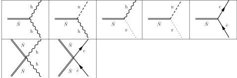
Figure 1: The vertices contributing to the renormalization of shift-dependent operators at one-loop.

The second ingredient needed for the computation are vertices describing the interaction of external $\bar{N}^{i}$-legs with the dynamical fields. The relevant vertices are depicted in Fig. 1 and are obtained by expanding the Lagrangian up to the given order in the number of fields. The corresponding formulas are rather lengthy and are relegated to the Appendix A.

The most important advantage of focusing on the renormalization of shift-dependent operators is that all vertices come exclusively from the kinetic terms and are completely independent of the structure of the potential, as well as of the gauge parameters $\sigma$ and $\xi$. Interestingly, this implies that the vertices are universal for HG in any spacetime dimensions. Another implication is that they are independent of the couplings $\nu_{1},\nu_{2},\nu_{3}$. As the propagators (27) also do not contain these couplings, we conclude that the one-loop renormalization of $G$ and $\lambda$ is insensitive to them altogether.

III.4 One-loop diagrams

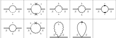
Figure 2: Logarithmically divergent Feynman diagrams contributing to the renormalization of $G$ and $\lambda$ at one-loop level.

We are interested in capturing the renormalization of the operators $\partial_{i}\bar{N}_{j}\partial_{i}\bar{N}_{j}$ and $(\partial_{i}\bar{N}_{i})^{2}$, which in momentum space read $p_{i}p_{i}\bar{N}_{j}\bar{N}_{j}$, $p_{i}p_{j}\bar{N}_{i}\bar{N}_{j}$, where $p_{i}$ denotes the momentum flowing through the $\bar{N}_{i}$-legs. The diagrams contributing to these operators are shown in Fig. 2. The prototypical form of the integrals appearing in the fish diagrams (upper row and first two diagrams in the lower row in the figure) is

$$\int\frac{\mathrm{d}\omega\mathrm{d}^{3}k}{(2\pi)^{4}}\,\Pi_{1}(\omega,{\bf k})\,\Pi_{2}(-\omega,-{\bf k}+{\bf p})\,Q(\omega,{\bf k},{\bf p})\;.$$ (29)

Here $\omega$ and ${\bf k}$ are the loop frequency and momentum, ${\bf p}$ is the external momentum, $\Pi_{1,2}$ are the propagators of the fields in the loop, and $Q$ is a polynomial in momenta and frequency coming from the vertices. The propagators and vertices carry tensor indices that we have suppressed. We have also used that the external frequency vanishes as the background shift $\bar{N}_{i}$ was chosen to be time-independent. Similarly, the tadpole diagrams (the last two diagrams in Fig. 2) contain integrals of the form,

$$\int\frac{\mathrm{d}\omega\mathrm{d}^{3}k}{(2\pi)^{4}}\,\Pi(\omega,{\bf k})\,Q(\omega,{\bf k},{\bf p})\;.$$ (30)

The above integrals feature logarithmic divergences that we want to extract. To this end, we Taylor expand the integrands in (29), (30) and focus on the terms quadratic in the external momentum $p_{i}$. Next we average over directions of the loop momentum using the standard formulas specified to $d=3$ dimensions Collins (1986),

$$\overline{k_{i_{1}}k_{i_{2}}...k_{i_{n}}}=\begin{cases}0~{},&\text{if $n$ is odd}\\ \frac{k^{n}}{n+1}T_{i_{1}i_{2}...i_{n}}\;,&\text{if $n$ is even}\end{cases}$$ (31)

where

$$T_{i_{1}i_{2}...i_{n}}=\frac{1}{n!}\left[\delta_{i_{1}i_{2}}...\delta_{i_{n-1}i_{n}}+\text{all permutations of the i's}\right]\;.$$ (32)

In this way we are left with a sum of terms containing various tensor structures multiplied by the integrals

$$\int\frac{\mathrm{d}\omega\mathrm{d}^{3}k}{(2\pi)^{4}}\,\omega^{2a}k^{2b}\big{(}{\cal P}_{I}(\omega,k)\big{)}^{A}\big{(}{\cal P}_{J}(\omega,k)\big{)}^{B}\;,$$ (33)

with constant exponents $a,b,A,B$. Here ${\cal P}_{I,J}$, $I,J\in\{tt,s,1,2\}$ are the pole structures listed in (28). Note that at most two different pole structures can appear in an individual integral. The exponents in (33) satisfy the relation

$$6+6a+2b-6A-6B=0\;,$$ (34)

so that the integrals are logarithmically divergent.

To regularize the UV divergences we use the Schwinger representation for each pole function,

$$\big{(}{\cal P}_{I}(\omega,k)\big{)}^{A}=\int_{0}^{\infty}\frac{\mathrm{d}s_{I}s_{I}^{A-1}}{\Gamma(A)}\,e^{-s_{I}({\cal P}_{I}(\omega,q))^{-1}}\;,$$ (35)

where $\Gamma(z)$ is the gamma-function. The integration over $\omega$ and ${\bf k}$ is then performed using the formula,

$$\int\frac{\mathrm{d}\omega\mathrm{d}^{3}k}{(2\pi)^{4}}\,\omega^{2a}k^{2b}\;e^{-U\omega^{2}-Vk^{6}}=\frac{1}{24\pi^{3}}\Gamma\left(a+\frac{1}{2}\right)\Gamma\left(\frac{b}{3}+\frac{1}{2}\right)U^{-a-\frac{1}{2}}\;V^{-\frac{b}{3}-\frac{1}{2}}\;.$$ (36)

Finally, if the resulting integral involves two Schwinger parameters, we integrate over one of them. Namely, we write,

$$\int_{0}^{\infty}\!\!\mathrm{d}s_{1}\mathrm{d}s_{2}\;s_{1}^{A-1}s_{2}^{B-1}(s_{1}+s_{2})^{-a-\frac{1}{2}}(s_{1}+u\,s_{2})^{-\frac{b}{3}-\frac{1}{2}}\!=\!\!\int_{0}^{\infty}\frac{\mathrm{d}s_{1}}{s_{1}}\!\int_{0}^{\infty}\!\!\mathrm{d}z\,\frac{z^{B-1}}{(1+z)^{a+\frac{1}{2}}(1+u\,z)^{\frac{b}{3}+\frac{1}{2}}}\,,$$ (37)

where we made the change of variables $z=s_{2}/s_{1}$ and used the relation (34). The integral over $z$ is convergent and for all values of $a,b,B$ appearing in our calculation can be taken in terms of elementary functions. The integral over the last remaining Schwinger parameter is kept to the end of the calculation and encodes the logarithmic divergence.

We have implemented the computational procedure described in this section in a Mathematica code. Manipulation of tensor objects was performed using the package xAct . Some parts of the computation were repeated using an alternative code written in FORM Vermaseren (2000). For a check of the procedure and the code we also performed the calculations in the case of $(2+1)$ dimensions where we reproduced the results of Barvinsky et al. (2017a).

IV The $\beta$-functions of $G$ and $\lambda$

Evaluation of the one-loop diagrams depicted in Fig. 2 produces a divergent correction to the effective Lagrangian for $\bar{N}^{i}$,

$$\delta{\cal L}_{\bar{N}}^{\rm 1-loop,\,div}=\Big{(}C_{1}\,p_{i}\bar{N}_{j}p_{i}\bar{N}_{j}+C_{2}\,(p_{i}\bar{N}_{i})^{2}\Big{)}\int\frac{\mathrm{d}s}{s}\;.$$ (38)

Comparing this with (15) we extract the renormalized couplings,

$$G_{R}=G-4G^{2}C_{1}\int\frac{\mathrm{d}s}{s}~{},~{}~{}~{}~{}~{}\lambda_{R}=\lambda+2G\big{(}(1-2\lambda)C_{1}-C_{2})\int\frac{\mathrm{d}s}{s}\;.$$ (39)

We interpret the logarithmic divergence as the result of integrating out high-momentum modes in the Wilsonian approach to renormalization. Thus, we identify,

$$\int\frac{\mathrm{d}s}{s}\simeq\log\left(\frac{\Lambda^{6}_{\rm UV}}{k_{*}^{6}}\right)\;,$$ (40)

where $\Lambda_{\rm UV}$ is a UV cutoff for momentum and $k_{*}$ is the RG reference scale. $\beta$-functions are defined as sensitivities of the couplings to $k_{*}$, which yields,

$$\beta_{G}\equiv\frac{dG_{R}}{d\log k_{*}}=24G^{2}C_{1}\;,$$ (41a)

$$\beta_{\lambda}\equiv\frac{d\lambda_{R}}{d\log k_{*}}=12G\big{(}C_{2}-(1-2\lambda)C_{1}\big{)}\;.$$ (41b)

The computation of the coefficients $C_{1,2}$ for general gauge parameter $\{\sigma,\xi,\varsigma\}$ is rather cumbersome due to the presence of four different pole structures in the propagators that generate a large number of terms for every diagram. The situation is simplified if one chooses the gauge parameters in such a way that some of the pole structures coincide. In this section we fix

$$\xi=-\frac{1-2\lambda}{2(1-\lambda)}\;,$$ (42)

which collapses the two poles corresponding to the gauge modes, ${\cal P}_{1}={\cal P}_{2}$. In order to keep track of the gauge (in)dependence of the result we allow the two remaining gauge parameters $\sigma,\varsigma$ to take arbitrary values. Results for two other choices of gauge are presented in Appendix B.

In the gauge (42) we obtain,

$$\beta_{G}= \frac{G^{2}}{40\pi^{2}\left(1+\sqrt{\alpha}\right)\sqrt{\alpha}(1-\lambda)(1-3\lambda)\sqrt{\nu_{5}}}\Big{[}-\alpha(1-3\lambda)\big{(}5(5-4\lambda)\sqrt{2\sigma\nu_{5}}+18-14\lambda\big{)}$$

$$-\sqrt{\alpha}\left(5(1-3\lambda)(5-4\lambda)\sqrt{2\sigma\nu_{5}}+53-142\lambda+99\lambda^{2}\right)-27+(74-57\lambda)\lambda\Big{]}\;,$$ (43)

$$\beta_{\lambda}= \frac{27(1-\lambda)^{2}+3\sqrt{\alpha}(11-3\lambda)(1-\lambda)-2\alpha(1-3\lambda)^{2}}{120\pi^{2}(1+\sqrt{\alpha})\sqrt{\alpha}(1-\lambda)}\frac{G}{\sqrt{\nu_{5}}}\;,$$ (44)

where we have introduced

$$\alpha=\frac{\nu_{s}}{\nu_{5}}\;.$$ (45)

We observe that both expressions are independent of the gauge parameter $\varsigma$. On the other hand, $\beta_{G}$ depends on $\sigma$. This is not unexpected. Indeed, a change of gauge is known to affect the background effective action by adding to it a contribution which is a linear combination of equations of motion DeWitt (1967); Kallosh (1974). Such terms vanish for on-shell background configurations, but not in general. The background used in our calculations is not on-shell, so the effective action evaluated on it is gauge-dependent. In Appendix C we show that a change of gauge induces the following shift of the renormalized couplings,

$$G\mapsto G-2G^{2}\epsilon~{},~{}~{}~{}~{}~{}\lambda\mapsto\lambda~{},~{}~{}~{}~{}~{}\nu_{a}\mapsto\nu_{a}-4G\nu_{a}\epsilon\;,$$ (46)

where $\epsilon$ is an infinitesimal parameter. We see that $G$, as well as $\nu_{a}$, transform non-trivially and therefore their renormalization and $\beta$-functions are not gauge-invariant. On the other hand, $\lambda$ remains untouched by (46). It represents an essential coupling of the theory and its $\beta$-function must be gauge-independent. This is indeed born out by our computation, see (44). Other essential couplings can be chosen, for example, as $G/\sqrt{\nu_{5}}$, $\alpha$ and $\nu_{a}/\nu_{5}$, $a=1,2,3$.

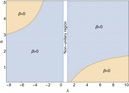
Figure 3: The sign of the $\beta$-function for the coupling $\lambda$ in different regions of parameter $(\lambda,\alpha)$. The $\beta$-function vanishes on the lines separating positive and negative regions. The line at $\lambda>1$ ($1/3<\lambda$) is UV attractive (repulsive) along the $\lambda$-direction. These lines correspond to potential location of fixed points of the full RG flow. The region $\lambda\in[1/3,1]$ is excluded by the requirement of unitarity.

Let us discuss the properties of the gauge-invariant function $\beta_{\lambda}$, eq. (44). Of particular interest is the manifold in the parameter space of the theory where this function vanishes. It constitutes a potential location of the fixed points of the full RG flow. The contribution of $G/\sqrt{\nu_{5}}$ factors out, so that the sign of $\beta_{\lambda}$ and the location of its zeros are determined only by two parameters $\lambda$ and $\alpha$. We have the following regions in the plane of these parameters, see Fig. 3:

• $\lambda<1/3~{},~{}~{}\alpha\leq 9/4$

  In this region $\beta_{\lambda}$ is always positive. So it does not contain any fixed points.

• $\lambda<1/3~{},~{}~{}\alpha>9/4$

  $\beta_{\lambda}$ is positive at $\lambda>\lambda_{\alpha}$ and negative at $\lambda<\lambda_{\alpha}$, where

  $$\lambda_{\alpha}=\frac{9+7\sqrt{\alpha}-2\alpha+2\sqrt{10(\alpha+\alpha^{3/2})}}{3(3+\sqrt{\alpha}-2\alpha)}\;.$$ (47)

  The $\beta$-function vanishes on the line $(\lambda_{\alpha},\alpha)$ which is IR attractive along the $\lambda$-direction.

• $\lambda>1~{},~{}~{}\alpha<9/4$

  $\beta_{\lambda}$ is positive at $\lambda<\lambda_{\alpha}$ and negative at $\lambda>\lambda_{\alpha}$, where $\lambda_{\alpha}$ is again given by (47). Now the line $(\lambda_{\alpha},\alpha)$ is attractive along the $\lambda$-direction in UV. When embedded into the full 6-dimensional space of the essential couplings of the theory, this line is promoted to a codimension-one surface. UV fixed points of the full RG flow, if any, should lie on this surface.

• $\lambda>1~{},~{}~{}\alpha\geq 9/4$

  Here $\beta_{\lambda}$ is always positive, and no fixed points exist in this region.

Presence of UV attractive zeros of $\beta_{\lambda}$ at finite values of $\lambda>1$ is analogous to the situation in $(2+1)$ dimensions, where such zero is known to correspond to an asymptotically free UV fixed point Barvinsky et al. (2017a).

To carry the comparison with the $(2+1)$-dimensional case further, it is instructive to work out the behavior of $\beta_{\lambda}$ when $\lambda$ approaches the boundaries of the allowed regions, $\lambda\to 1/3^{-}$ or $\lambda\to 1^{+}$, with all other couplings in the Lagrangian held fixed. As implied by (9b), these limits correspond to degenerate dispersion relation of the scalar graviton. One writes (see eqs. (10), (45)),

$$\alpha=\frac{1-\lambda}{1-3\lambda}\bigg{(}\frac{8\nu_{4}}{\nu_{5}}+3\bigg{)}\;.$$ (48)

Substituting this into the expression (44) one obtains,

$$\beta_{\lambda}\propto\sqrt{\frac{1}{3}-\lambda} \text{at}~{}\lambda\to\frac{1}{3}^{-}\;,$$ (49a)

$$\beta_{\lambda}\propto\frac{1}{\sqrt{\lambda-1}} \text{at}~{}\lambda\to 1^{+}\;.$$ (49b)

In other words, the $\beta$-function of $\lambda$ vanishes (diverges) as the square-root when the frequency of the scalar graviton diverges (vanishes). This is the same qualitative behavior as in $(2+1)$ dimensions, see eq. (22a) of Barvinsky et al. (2017a).

V Conclusions

In this paper we have computed the renormalization group flow of $G$ and $\lambda$ in $(3+1)$-dimensional Hořava Gravity. We used the background-field method and exploited the gauge invariance of the kinetic term which allowed us to focus on the renormalization of operators constructed from the shift field. Setting the spatial background metric to be flat we avoided major complications arising due to the involved structure of the potential term. We have considered a variety of gauge choices and found that the $\beta$-function of $G$ depends on the gauge, as expected given that this coupling is not essential, i.e. it cannot be defined using only on-shell quantities.

On the other hand, the coupling $\lambda$ is essential and its $\beta$-function given by eq. (44) is gauge-independent. $\beta_{\lambda}$ vanishes on two disjoint codimension-one surfaces in the 6-dimensional parameter space of essential couplings. One of these surfaces is UV attractive along the $\lambda$-direction, whereas the other is UV repulsive. The former surface represents a potential location for UV fixed points of the full RG flow. Of course, to make a definitive conclusion about the existence of such fixed points one has to calculate $\beta$-functions of the remaining couplings of the theory that enter in the potential part of the action. This calculation will require other methods than the ones used in this paper and we plan to report it elsewhere.

As a final remark, we note that the approach described in this paper can be straightforwardly generalized to compute the running of $G$ and $\lambda$ in any number of spacetime dimensions $(d+1)$. Indeed, all interaction vertices used in our calculation come from the kinetic term in the action and the part of the gauge-fixing term that contains the shift field. These are universal. The dimension-dependent potential entered in the calculation only via its quadratic expansion that determined the propagators of the dynamical fields. This quadratic part can be reconstructed for arbitrary $d$ from the requirements of invariance under the Lifshitz scaling and the linearized spatial diffeomorphisms and will be fully characterized by the combination of couplings appearing in the dispersion relations of the physical modes.

Appendix A Interaction Lagrangian

Here we present explicitly the parts of the interaction Lagrangian that are relevant for the one-loop renormalization of the operators in the background action (15). These are obtained from the total action (25) and are of two types. First, there are cubic interactions including one $\bar{N}^{i}$, with or without spatial derivatives, and two dynamical fields:

$${\cal L}_{\bar{N}hh}=\frac{1}{2G}\bigg{[} -\frac{1}{4}\bar{N}_{ij}h\dot{h}_{ij}-\frac{\lambda}{2}\bar{N}_{ij}h_{ij}\dot{h}+\bar{N}_{k}\partial_{i}h_{jk}\dot{h}_{ij}-\frac{1}{2}\bar{N}_{k}\partial_{k}h_{ij}\dot{h}_{ij}-\lambda\bar{N}_{k}\partial_{i}h_{ik}\dot{h}$$

$$+\frac{\lambda}{2}\bar{N}_{k}\partial_{k}h\dot{h}-\bar{N}_{k}\partial_{l}h_{li}\dot{h}_{ik}+\lambda\bar{N}_{k}\partial_{i}h\dot{h}_{ik}\bigg{]},$$ (50a)

$${\cal L}_{\bar{N}hn}=\frac{1}{2G}\bigg{[} -\bar{N}_{ij}\partial_{i}h_{jk}n_{k}+\frac{1}{2}\bar{N}_{ij}\partial_{k}h_{ij}n_{k}+\frac{1}{2}\bar{N}_{ij}h\partial_{i}n_{j}-\bar{N}_{ij}h_{ki}\partial_{k}n_{j}-\bar{N}_{ij}h_{ik}\partial_{j}n_{k}$$

$$+2\lambda\partial_{i}\bar{N}_{i}\partial_{j}h_{jk}n_{k}-\lambda\partial_{i}\bar{N}_{i}\partial_{k}hn_{k}+2\lambda\partial_{i}\bar{N}_{i}h_{jk}\partial_{j}n_{k}-\lambda\partial_{i}\bar{N}_{i}h\partial_{k}n_{k}$$

$$+2\lambda\partial_{i}\bar{N}_{j}h_{ij}\partial_{k}n_{k}-\bar{N}_{k}\partial_{i}h_{jk}\partial_{i}n_{j}-\bar{N}_{k}\partial_{i}h_{jk}\partial_{j}n_{i}+\bar{N}_{k}\partial_{k}h_{ij}\partial_{i}n_{j}$$

$$+2\lambda\bar{N}_{k}\partial_{l}h_{lk}\partial_{i}n_{i}-\lambda\bar{N}_{k}\partial_{k}h\partial_{i}n_{i}+\partial_{j}\bar{N}_{i}\partial_{l}h_{li}n_{j}-\lambda\partial_{j}\bar{N}_{i}\partial_{i}hn_{j}$$

$$-\bar{N}_{k}\partial_{l}h_{li}\partial_{k}n_{i}+\lambda\bar{N}_{k}\partial_{i}h\partial_{k}n_{i}-\frac{\varsigma}{2}\bar{N}_{ij}\partial_{k}h_{ki}n_{j}+\frac{\varsigma\lambda}{2}\bar{N}_{ij}\partial_{i}hn_{j}\bigg{]},$$ (50b)

$${\cal L}_{\bar{N}\pi h}=\frac{i}{G}\bar{N}_{k} \pi_{i}\dot{h}_{ik}\;,$$ (50c)

$${\cal L}_{\bar{N}\pi n}=\frac{1}{2G}\big{[} -2i\partial_{j}\bar{N}_{i}\pi_{i}n_{j}+2i\bar{N}_{k}\pi_{i}\partial_{k}n_{i}+i\varsigma\bar{N}_{ij}\pi_{i}n_{j}\big{]}\;,$$ (50d)

$${\cal L}_{\bar{N}\bar{c}c}=-\frac{1}{G}\bigg{[} -2\bar{N}_{k}\bar{c}_{i}\partial_{k}\dot{c}_{i}+2\partial_{k}\bar{N}_{i}\bar{c}_{i}\dot{c}_{k}-\frac{\varsigma}{2}\bar{N}_{ij}\bar{c}_{i}\dot{c}_{j}\bigg{]}\;,$$ (50e)

where $\bar{N}_{ij}\equiv\partial_{i}\bar{N}_{j}+\partial_{j}\bar{N}_{i}$ and in deriving (50a) we eliminated some terms that combine into a total time derivative. Second, we need the quartic interactions involving two $\bar{N}_{i}$ and two dynamical fields. In this case divergent contributions come from tadpole diagrams where the two lines of the dynamical fields stemming from the same vertex connect with each other to form a loop. Thus, to find the divergent contributions of the form (15), we can restrict only to those terms in the quartic Lagrangian that contain exactly two spatial derivatives acting on the $\bar{N}_{i}$-legs. These have the form,

$${\cal L}_{\bar{N}\bar{N}hh}=\frac{1}{2G}\bigg{[} \bar{N}_{ij}^{2}\bigg{(}-\frac{1}{16}h_{kl}^{2}+\frac{h^{2}}{32}\bigg{)}+\frac{1}{2}\bar{N}_{ij}\bar{N}_{kj}h_{il}h_{kl}-\frac{1}{4}\bar{N}_{ij}\bar{N}_{kj}h_{ik}h+\frac{1}{4}\bar{N}_{ij}\bar{N}_{kl}h_{ik}h_{jl}$$

$$-\!\lambda(\partial_{i}\bar{N}_{i})^{2}\bigg{(}\!\!-\!\frac{1}{4}h_{kl}^{2}+\!\frac{h^{2}}{8}\bigg{)}\!-\!\frac{\lambda}{4}\bar{N}_{ij}\bar{N}_{kl}h_{ij}h_{kl}+\!\frac{\lambda}{2}\bar{N}_{ij}\partial_{k}\bar{N}_{k}h_{ij}h\!-\!\lambda\bar{N}_{ij}\partial_{k}\bar{N}_{k}h_{il}h_{jl}\bigg{]},$$ (51a)

$${\cal L}_{\bar{N}\bar{N}\bar{c}c}=-\frac{1}{G}\bigg{[} -\bar{N}_{k}\partial_{k}\partial_{l}\bar{N}_{i}\bar{c}_{i}c_{l}+\partial_{k}\bar{N}_{i}\partial_{l}\bar{N}_{k}\bar{c}_{i}c_{l}-\frac{\varsigma}{2}\bar{N}_{ij}\partial_{k}\bar{N}_{j}\bar{c}_{i}c_{k}\bigg{]}\;.$$ (51b)

Appendix B Alternative gauges

In this appendix we report the results of the computation in two gauges outside the family considered in Sec. IV. In both cases the gauge parameters $\sigma,\xi$ are chosen in the way to reduce the number of pole structures by making the gauge poles coincide with the poles of the physical modes. The third parameter $\varsigma$ is kept arbitrary.

• The first choice is

  $$\sigma=\frac{1}{2\nu_{5}}~{},~{}~{}~{}~{}~{}\xi=\frac{\nu_{s}}{2\nu_{5}(1-\lambda)}-1~{}~{}~{}~{}\Longrightarrow~{}~{}~{}~{}{\cal P}_{1}={\cal P}_{tt},~{}{\cal P}_{2}={\cal P}_{s}\;.$$ (52)

  It leads to the following $\beta$-function for the coupling $G$,

  $$\beta_{G}=-\frac{32-89\lambda+57\lambda^{2}+3\sqrt{\alpha}(26-79\lambda+53\lambda^{2})+2\alpha(19-74\lambda+51\lambda^{2})}{40\pi^{2}(1+\sqrt{\alpha})\sqrt{\alpha}(1-\lambda)(1-3\lambda)}\frac{G^{2}}{\sqrt{\nu_{5}}}\;,$$ (53)

  where $\alpha$ is defined in (45).

• The second choice,

  $$\sigma=\frac{1}{2\nu_{s}}~{},~{}~{}~{}~{}~{}\xi=\frac{\nu_{5}}{2\nu_{s}(1-\lambda)}-1\;,~{}~{}~{}~{}\Longrightarrow~{}~{}~{}~{}{\cal P}_{1}={\cal P}_{s},~{}{\cal P}_{2}={\cal P}_{tt}\;,$$ (54)

  yields

  $$\beta_{G}=-\frac{47-154\lambda+117\lambda^{2}+3\sqrt{\alpha}(26-79\lambda+53\lambda^{2})+a(23-83\lambda+42\lambda^{2})}{40\pi^{2}(1+\sqrt{\alpha})\sqrt{\alpha}(1-\lambda)(1-3\lambda)}\frac{G^{2}}{\sqrt{\nu_{5}}}\;.$$ (55)

We observe that while $\beta_{G}$ is independent of $\varsigma$, it is different in the two gauges, as expected from the gauge-dependence of the renormalized Lagrangian.

On the other hand, we have found that the $\beta$-function of $\lambda$ is the same in both gauges (52), (54) and coincides with the expression (44) from the main text. Thus gauge-independence provides a further check of our calculational procedure.

Appendix C Ambiguity of the one-loop effective action

It is well-known that in gauge theories the background effective action $\Gamma_{\rm eff}$ depends on the choice of gauge fixing for the fluctuating fields, unless the background satisfies the equations of motion. This dependence is expressed by the statement that a change in the gauge fixing leads to the shift of the effective action,

$$\Gamma_{\rm eff}\mapsto\Gamma_{\rm eff}+\epsilon{\cal A}\;,$$ (56)

where $\epsilon$ is an infinitesimal parameter and ${\cal A}$ is a functional of the background fields which is a linear combination of the equations of motion DeWitt (1967); Kallosh (1974). Our task is to see if such a functional exists in the projectable HG. To be in line with the main text, we work in Euclidean time and focus on the high-energy part of the action given by (II).

As we are interested only in the one-loop divergence of $\Gamma_{\rm eff}$ which is an integral of a local Lagragian density, the functional ${\cal A}$ must also have this form. Moreover, it should be invariant under FDiff and contain only marginal operators with respect to the Lifshitz scaling. Variation of (II) with respect to $N^{i}$ and $\gamma_{ij}$ produces the equations,

$$\nabla_{j}K^{j}_{i}-\lambda\nabla_{i}K=0\;,$$ (57a)

$$-\!\frac{\partial}{\partial\tau}\big{[}\sqrt{\gamma}\big{(}K^{ij}\!-\!\lambda\gamma^{ij}K\big{)}\big{]}\!-\!2\sqrt{\gamma}\big{(}K^{i}_{k}K^{kj}\!-\!\lambda K^{ij}K\big{)}\!+\!\frac{1}{2}\sqrt{\gamma}\,\gamma^{ij}\big{(}K_{kl}K^{kl}\!-\!\lambda K^{2}\big{)}\!+\!\frac{\delta(\sqrt{\gamma}\,{\cal V})}{\delta\gamma_{ij}}=0\,,$$ (57b)

where for simplicity we set $N^{i}$ to zero by a choice of gauge. Wo do not write explicitly the result of the variation of the potential term which is too lengthy. The l.h.s. of the first equation is a vector operator of dimension 4. Any other local covariant vector operator in the theory has at least dimension 3 (this is the case for $\nabla_{i}R$). Thus, we cannot use the l.h.s. of (57a) to construct a local Lagrangian density of dimension 6.

On the other hand, the l.h.s. of (57b) already has dimension 6. To get a scalar density under FDiff we contract it with $\gamma_{ij}$. This yields,

$$-(1-3\lambda)\frac{\partial(\sqrt{\gamma}K)}{\partial\tau}+\frac{3}{2}\sqrt{\gamma}\big{(}K_{ij}K^{ij}-\lambda K^{2}\big{)}+\gamma_{ij}\frac{\delta(\sqrt{\gamma}\,{\cal V})}{\delta\gamma_{ij}}=0\;.$$ (58)

The last term on the l.h.s. represents the result of the variation of the potential part with respect to spatial Weyl transformations, $\gamma_{ij}\mapsto\Omega\gamma_{ij}$. By inspection of the expression (II), we find that for Weyl rescalings with a space-independent factor $\Omega$ the potential part transforms as $\sqrt{\gamma}\,{\cal V}\mapsto\Omega^{-3/2}\sqrt{\gamma}\,{\cal V}$. This implies that for a general rescaling the variation of $\sqrt{\gamma}\,{\cal V}$ has the form,

$$\gamma_{ij}\frac{\delta(\sqrt{\gamma}\,{\cal V})}{\delta\gamma_{ij}}=-\frac{3}{2}\sqrt{g}\,{\cal V}+(\text{total spatial derivatives})\;.$$ (59)

Therefore, the l.h.s. of (58) can be written as

$$\frac{3}{2}\sqrt{\gamma}\big{(}K_{ij}K^{ij}-\lambda K^{2}-{\cal V}\big{)}+(\text{total derivatives})\;.$$ (60)

Integrating over the whole spacetime and neglecting total derivatives one obtains,

$${\cal A}=\int\mathrm{d}\tau\mathrm{d}^{3}x\sqrt{\gamma}\,\Big{(}K_{ij}K^{ij}-\lambda K^{2}-{\cal V}\Big{)}\;.$$ (61)

Adding it to the effective action as in (56) induces a shift of the couplings (46) discussed in the main text.

Let us mention another way to arrive to the expression (61). Namely, one can restore time reparameterizations by reintroducing in (II) the lapse function $N(t)$. Then variation with respect to $N$ produces a global Hamiltonian constraint,

$$\int\mathrm{d}^{3}x\sqrt{\gamma}\,\big{(}K_{ij}K^{ij}-\lambda K^{2}-{\cal V}\big{)}=0\;.$$ (62)

Clearly, setting $N$ back to 1 and integrating the l.h.s. of this equation over time we recover (61).

References

- Donoghue (1994) J. F. Donoghue, Phys. Rev. D50, 3874 (1994), arXiv:gr-qc/9405057 [gr-qc] .
- Burgess (2004) C. P. Burgess, Living Rev. Rel. 7, 5 (2004), arXiv:gr-qc/0311082 [gr-qc] .
- Donoghue et al. (2017) J. F. Donoghue, M. M. Ivanov, and A. Shkerin, “EPFL Lectures on General Relativity as a Quantum Field Theory,” (2017), arXiv:1702.00319 [hep-th] .
- Stelle (1977) K. S. Stelle, Phys. Rev. D16, 953 (1977).
- Fradkin and Tseytlin (1981) E. S. Fradkin and A. A. Tseytlin, Phys. Lett. 104B, 377 (1981).
- Avramidi and Barvinsky (1985) I. G. Avramidi and A. O. Barvinsky, Phys. Lett. 159B, 269 (1985).
- Stelle (1978) K. S. Stelle, Gen. Rel. Grav. 9, 353 (1978).
- Woodard (2015) R. P. Woodard, Scholarpedia 10, 32243 (2015), arXiv:1506.02210 [hep-th] .
- Hořava (2009) P. Hořava, Phys. Rev. D79, 084008 (2009), arXiv:0901.3775 [hep-th] .
- Mukohyama (2010) S. Mukohyama, Class. Quant. Grav. 27, 223101 (2010), arXiv:1007.5199 [hep-th] .
- Sotiriou (2011) T. P. Sotiriou, Proceedings, 14th Conference on Recent developments in gravity (NEB 14): Ioannina, Greece, June 8-11, 2010, J. Phys. Conf. Ser. 283, 012034 (2011), arXiv:1010.3218 [hep-th] .
- Blas (2018) D. Blas, Proceedings, Workshop CPT and Lorentz Symmetry in Field Theory: Faro, Portugal, July 6-7, 2017, J. Phys. Conf. Ser. 952, 012002 (2018).
- Wang (2017) A. Wang, Int. J. Mod. Phys. D26, 1730014 (2017), arXiv:1701.06087 [gr-qc] .
- Blas et al. (2010) D. Blas, O. Pujolas, and S. Sibiryakov, Phys. Rev. Lett. 104, 181302 (2010), arXiv:0909.3525 [hep-th] .
- Blas and Lim (2015) D. Blas and E. Lim, Int. J. Mod. Phys. D23, 1443009 (2015), arXiv:1412.4828 [gr-qc] .
- Abbott et al. (2017) B. P. Abbott et al. (LIGO Scientific, Virgo, Fermi-GBM, INTEGRAL), Astrophys. J. 848, L13 (2017), arXiv:1710.05834 [astro-ph.HE] .
- Emir Gümrükçüoğlu et al. (2018) A. Emir Gümrükçüoğlu, M. Saravani, and T. P. Sotiriou, Phys. Rev. D97, 024032 (2018), arXiv:1711.08845 [gr-qc] .
- Blas et al. (2011) D. Blas, O. Pujolas, and S. Sibiryakov, JHEP 04, 018 (2011), arXiv:1007.3503 [hep-th] .
- Blas and Sibiryakov (2011a) D. Blas and S. Sibiryakov, JCAP 1107, 026 (2011a), arXiv:1104.3579 [hep-th] .
- Audren et al. (2013) B. Audren, D. Blas, J. Lesgourgues, and S. Sibiryakov, JCAP 1308, 039 (2013), arXiv:1305.0009 [astro-ph.CO] .
- Chadha and Nielsen (1983) S. Chadha and H. B. Nielsen, Nucl. Phys. B217, 125 (1983).
- Anber and Donoghue (2011) M. M. Anber and J. F. Donoghue, Phys. Rev. D83, 105027 (2011), arXiv:1102.0789 [hep-th] .
- Sundrum (2012) R. Sundrum, Phys. Rev. D86, 085025 (2012), arXiv:1106.4501 [hep-th] .
- Kiritsis (2013) E. Kiritsis, JHEP 01, 030 (2013), arXiv:1207.2325 [hep-th] .
- Bednik et al. (2013) G. Bednik, O. Pujolas, and S. Sibiryakov, JHEP 11, 064 (2013), arXiv:1305.0011 [hep-th] .
- Kharuk and Sibiryakov (2016) I. Kharuk and S. M. Sibiryakov, Theor. Math. Phys. 189, 1755 (2016), [Teor. Mat. Fiz.189,no.3,405(2016)], arXiv:1505.04130 [hep-th] .
- Groot Nibbelink and Pospelov (2005) S. Groot Nibbelink and M. Pospelov, Phys. Rev. Lett. 94, 081601 (2005), arXiv:hep-ph/0404271 [hep-ph] .
- Bolokhov et al. (2005) P. A. Bolokhov, S. Groot Nibbelink, and M. Pospelov, Phys. Rev. D72, 015013 (2005), arXiv:hep-ph/0505029 [hep-ph] .
- Liberati (2013) S. Liberati, Class. Quant. Grav. 30, 133001 (2013), arXiv:1304.5795 [gr-qc] .
- Blas and Sibiryakov (2011b) D. Blas and S. Sibiryakov, Phys. Rev. D84, 124043 (2011b), arXiv:1110.2195 [hep-th] .
- Barvinsky et al. (2016) A. O. Barvinsky, D. Blas, M. Herrero-Valea, S. M. Sibiryakov, and C. F. Steinwachs, Phys. Rev. D93, 064022 (2016), arXiv:1512.02250 [hep-th] .
- Blas et al. (2009) D. Blas, O. Pujolas, and S. Sibiryakov, JHEP 10, 029 (2009), arXiv:0906.3046 [hep-th] .
- Koyama and Arroja (2010) K. Koyama and F. Arroja, JHEP 03, 061 (2010), arXiv:0910.1998 [hep-th] .
- Izumi and Mukohyama (2011) K. Izumi and S. Mukohyama, Phys. Rev. D84, 064025 (2011), arXiv:1105.0246 [hep-th] .
- Gumrukcuoglu et al. (2012) A. E. Gumrukcuoglu, S. Mukohyama, and A. Wang, Phys. Rev. D85, 064042 (2012), arXiv:1109.2609 [hep-th] .
- Barvinsky et al. (2018) A. O. Barvinsky, D. Blas, M. Herrero-Valea, S. M. Sibiryakov, and C. F. Steinwachs, JHEP 07, 035 (2018), arXiv:1705.03480 [hep-th] .
- Barvinsky et al. (2017a) A. O. Barvinsky, D. Blas, M. Herrero-Valea, S. M. Sibiryakov, and C. F. Steinwachs, Phys. Rev. Lett. 119, 211301 (2017a), arXiv:1706.06809 [hep-th] .
- Benedetti and Guarnieri (2014) D. Benedetti and F. Guarnieri, JHEP 03, 078 (2014), arXiv:1311.6253 [hep-th] .
- Griffin et al. (2017) T. Griffin, K. T. Grosvenor, C. M. Melby-Thompson, and Z. Yan, JHEP 06, 004 (2017), arXiv:1701.08173 [hep-th] .
- D’Odorico et al. (2014) G. D’Odorico, F. Saueressig, and M. Schutten, Phys. Rev. Lett. 113, 171101 (2014), arXiv:1406.4366 [gr-qc] .
- Sotiriou et al. (2009) T. P. Sotiriou, M. Visser, and S. Weinfurtner, Phys. Rev. Lett. 102, 251601 (2009), arXiv:0904.4464 [hep-th] .
- Abbott (1982) L. F. Abbott, Acta Phys. Polon. B13, 33 (1982).
- Barvinsky and Vilkovisky (1985) A. O. Barvinsky and G. A. Vilkovisky, Phys. Rept. 119, 1 (1985).
- D’Odorico et al. (2015) G. D’Odorico, J.-W. Goossens, and F. Saueressig, JHEP 10, 126 (2015), arXiv:1508.00590 [hep-th] .
- Barvinsky et al. (2017b) A. O. Barvinsky, D. Blas, M. Herrero-Valea, D. V. Nesterov, G. Pérez-Nadal, and C. F. Steinwachs, JHEP 06, 063 (2017b), arXiv:1703.04747 [hep-th] .
- Collins (1986) J. C. Collins, Renormalization, Cambridge Monographs on Mathematical Physics, Vol. 26 (Cambridge University Press, Cambridge, 1986).
- Vermaseren (2000) J. A. M. Vermaseren, “New features of FORM,” (2000), arXiv:math-ph/0010025 [math-ph] .
- DeWitt (1967) B. S. DeWitt, Phys. Rev. 162, 1195 (1967).
- Kallosh (1974) R. E. Kallosh, Nucl. Phys. B78, 293 (1974).