Improving Discrete Latent Representations
With Differentiable Approximation Bridges

Abstract

Modern neural network training relies on piece-wise (sub-)differentiable functions in order to use backpropagation to update model parameters. In this work, we introduce a novel method to allow simple non-differentiable functions at intermediary layers of deep neural networks. We do so by training with a differentiable approximation bridge (DAB) neural network which approximates the non-differentiable forward function and provides gradient updates during backpropagation. We present strong empirical results (performing over 600 experiments) in four different domains: unsupervised (image) representation learning, variational (image) density estimation, image classification, and sequence sorting to demonstrate that our proposed method improves state of the art performance. We demonstrate that training with DAB aided discrete non-differentiable functions improves image reconstruction quality and posterior linear separability by 10% against the Gumbel-Softmax relaxed estimator [37, 26] as well as providing a 9% improvement in the test variational lower bound in comparison to the state of the art RELAX [16] discrete estimator. We also observe an accuracy improvement of 77% in neural sequence sorting and a 25% improvement against the straight-through estimator [5] in an image classification setting. The DAB network is not used for inference and expands the class of functions that are usable in neural networks.

1 Introduction

Deep neural networks have advanced the state of the art in object recognition [21, 46], machine translation [9], and game playing [45], however they generally only function over the range of numerical values encountered during training [48]. In contrast, traditional (non-learned) algorithms, such as Merge-Sort [27], are provably stable and can deal with arbitrary inputs. In this work, we introduce a novel formulation that allows for the incorporation of simple non-differentiable functions, such as Merge-Sort, Signum and K-Means in neural network pipelines.

Most state of the art neural networks [21, 46, 15] rely on some variant of Robbins-Monroe [44] based stochastic optimization. The requirement for utilizing this algorithm includes the assumption that the gradients of the functional be Lipschitz continuous. In contrast, some of the most common functions used in neural networks, the ReLU activation [1] and the Max-Pooling layer [57] are not fully differentiable. In general, this problem is circumvented by ignoring the measure zero non-differentiable domain or through the use of the adjoint method. Functions such as sort and k-means are not amenable to a similar treatment.

In this work, we study approximate gradient pathways that allow for simple non-differentiable functions as sub-modules of neural networks. We validate DAB using the sort, top-k, k-means, signum, binary-threshold and non-reparameterized bernoulli non-differentiable functions and demonstrate competitive performance on a variety of tasks. DAB enables the use of these functions by introducing a smooth neural network approximation to the non-differentiable function; the gradients of the DAB network are then used at training time to update previous layers of the network. The DAB network is trained jointly with the central optimization objective and creates its approximation via the introduction of a regularizer (Section 3). At inference, the DAB network is removed, thus requiring no extra memory or compute after training.

2 Related Work

	Method / Objective	Supports Non-Differentiable Functions	Scales to Large Dimensions	Works with Operators that Change Dimension	Typical Unique Hyper Parameters
DNI [25] / DPG [24] / DGL [4]	Asynchronous network updates.	no	yes	yes	-
Gradient Free Methods [51, 28, 14, 2, 10, 11, 35]	Optimize arbitrary functions.	yes	no	yes	-
Score Function Estimator [13, 32]	Differentiate non-differentiable functions.	yes	no	yes	0
Straight-Through Estimator [5]	Ignore non-differentiable functions.	yes	yes	no	0
Relaxed Estimators [37, 26, 49, 16]	Relaxed approximations to non-differentiable functions.	yes	yes	yes	1 - 3
DAB (ours)	Differentiate non-differentiable functions.	yes	yes	yes	1

Traditional Solutions: Traditional solutions to handling non-differentiable functions in machine learning include using the score function estimator (SFE) [13, 32] (also known as REINFORCE [56]), the straight-through estimator (STE) [5], or the reparameterization path-wise estimator [30]. While the SFE is an unbiased estimate of the gradients, it generally suffers from high variance [16] and needs to be augmented with control variates [12] that require manual tuning and domain knowledge. The STE on the other hand is a solution that simply copies gradients back, skipping the non-differentiable portion (i.e. treating it as an identity operation). Furthermore, the STE does not allow for operators that change dimension, i.e. $f:\mathbb{R}^{A}\mapsto\mathbb{R}^{B},A\neq B$, since it is unclear how the gradients of the larger/smaller output would be copied back. In contrast to the SFE, the reparameterization trick used in variational autoencoders (VAE) [30], enables differentiating through distributions by reframing the expectation with respect to a variable that is not part of the computational graph. The difference between the SFE and the reparameterization trick can be understood by analyzing how they estimate gradients:

SFE: $\!\begin{aligned} \nabla_{\theta}\mathbb{E}_{q_{\theta}}[f(z)]=\mathbb{E}_{q_{\theta}}[f(z)\nabla_{\theta}\log q_{\theta}(z)]\end{aligned}$

Reparameterization: $\!\begin{aligned} \nabla_{\theta}\mathbb{E}_{q_{\theta}}[f(z)]=\mathbb{E}_{p(\epsilon)}[\nabla_{\theta}f(z)]\end{aligned}$

The reparameterization path-wise estimator takes into account how the derivative of the function, $f(z)$, is modulated by the choice of measure, $q_{\theta}$, while the SFE treats the function, $f(z)$, as a black box. See [39] for a thorough treatment on the topic.

Relaxed Differentiability: While the reparameterization estimator has lower variance than the SFE, it did not afford a discrete reparameterization until recently. The Gumbel-Softmax relaxed estimator (simultaneously proposed in [37, 26]) for the Bernouilli and Discrete distributions anneals a softmax with additive Gumbel noise until it eventually converges to the corresponding ‘hard’ distribution. This technique can be interpreted as a form of bias-variance trade-off [37]. More recently, REBAR [49] and RELAX [16] were proposed to combine both the SFE and the reparameterization trick in order to produce a new estimator with lower variance. RELAX [16] differs from REBAR [49] by using a learned Q function [55] neural network as a control variate. We empirically contrast our estimator against Gumbel-Softmax in Experiment 4.2 and RELAX and REBAR in Experiment 4.2.1, demonstrating improved performance using three different metrics.

Gradient Free Methods: Machine learning has a rich history of backpropagation alternatives, ranging from simulated annealing [51], particle swarm optimization [28], genetic algorithms [14], evolutionary strategies [2], and Bayesian approaches such as MCMC based sampling algorithms [10, 11]. These algorithms have been shown [43] to not scale to complex, large dimension optimization problems in large neural network models. More recent work in the analysis of backpropagation alternatives [35] has demonstrated the possibility of learning weight updates through the use of random matrices; however, no statement was made about training / convergence time.

Figure 1: Demonstration of a simple DAB approximation: scatter plots visualize test predictions and gradients of a multi-layer dense network fitting an $\epsilon$-margin signum function ($\epsilon=0.5$) over an input space of U(-1, 1). Left: Near beginning of training. Middle: Mid-way through training. Right: End of training.

Asynchronous Neural Network Updates: Recent work such as decoupled neural interfaces (DNI) [25] and decoupled parallel backpropagation (DPG) [24] introduced an auxiliary network to approximate gradients in RNN models. Similar approximation techniques have been introduced [4] (DGL) to allow for greedy layerwise CNN based training. The central objective with these models is to enable asynchronous updates to speed up training time. Our work differs from all of these solutions in that our objective is not to improve training speed / parallelism, but to learn a function approximator of a non-differentiable function such that it provides a meaningful training signal for the preceding layers in the network. This approach allows us to utilize non-differentiable functions such as kmeans, sort, signum, etc, as intermediary layers in neural network pipelines.

3 Model

Figure 2: Model of our proposed framework. $\color[rgb]{1,0,0}\definecolor[named]{pgfstrokecolor}{rgb}{1,0,0}l_{hard}$ represents the non-differentiable function and $\color[rgb]{1,0,0}\definecolor[named]{pgfstrokecolor}{rgb}{1,0,0}z_{hard}$ its outputs.

Given a set of training input images, $X_{tr}=\{x_{i}\}_{i=0}^{N},\ x_{i}\in\mathbb{R}^{M\times M}$, coupled with related ground-truth labels, $Y_{tr}=\{y_{i}\}_{i=0}^{N},\ y_{i}\in\mathbb{R}^{J}\text{(for classification) or }y_{i}\in\mathbb{R}^{M\times M}\text{(for autoencoding)}$, our objective is to learn the parameters, $\theta$, of a model, $f_{\theta}:x_{i}\mapsto y_{i}$, such that we generalize well on a hold-out test set, $\{X_{te},Y_{te}\}$, evaluated with a predefined metric, $\mathcal{M}(f_{\theta}(X_{te}),Y_{te})$. We focus on the case where the parameters $\theta$ are optimized using stochastic gradient descent [44], operating on a differentiable loss function $\mathcal{L}(f_{\theta}(X_{tr}),Y_{tr})$.

We begin by decomposing our model, $f_{\theta}$, into a layer-wise representation, $f_{\theta}=l_{\theta_{3}}\circ l_{\theta_{2}}\circ l_{\theta_{1}}$. We represent the output of each of the above layers as $\{z_{3},z_{2},z_{1}\}$ respectively. In this work we explore replacing the differentiable function $l_{\theta_{2}}$ with a non-differentiable version, ${\color[rgb]{1,0,0}\definecolor[named]{pgfstrokecolor}{rgb}{1,0,0}l_{hard}}$. Directly swapping ${\color[rgb]{1,0,0}\definecolor[named]{pgfstrokecolor}{rgb}{1,0,0}l_{hard}}$ for $l_{\theta_{2}}$ is not viable since it would prevent backpropagation gradient updates of $l_{\theta_{1}}$.

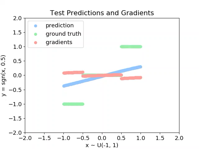
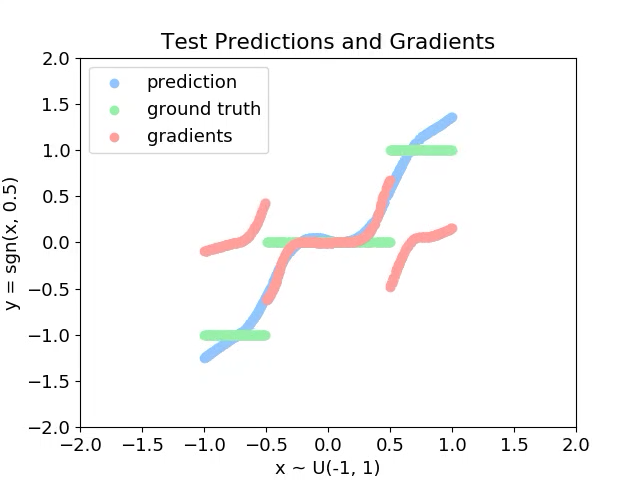
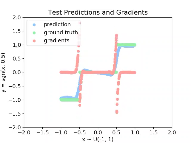
In order to circumvent this, we draw inspiration by visualizing what a typical multi-layer dense neural network does when it fits an output that is discontinuous. In Figure 1 we visualize three (test) snapshots of a network during training. The ground truth target, $y_{i}$, is an $\epsilon$-margin signum function, $y_{i}=sgn(x_{i},\epsilon)$, where $x_{i}\sim U(-1,1)$ and $\epsilon=0.5$.

$$sgn(x_{i},\epsilon) =\begin{cases}-1&x_{i}<-\epsilon\\ 0&x_{i}\in[-\epsilon,\epsilon]\\ 1&x_{i}>\epsilon\end{cases}$$ (1)

We train a small three layer ELU dense network using Adam [29] and use the final layer’s (un-activated) output in a least-square loss, $\mathcal{L}=||y_{i}-f_{\theta}(x_{i})||^{2}_{2}$. Neural networks have been extensively used to interpolate latent space in models such as variational autoencoders [30] and Word2Vec [38]. These interpolations are possible because neural networks learn a smooth K-Lipschitz mapping to transform the inputs to their target outputs, which implies smooth gradients. We rely on this property and introduce the DAB network, $l_{\phi}$.

The DAB network receives $z_{1}$ from the previous layer, $z_{1}=l_{\theta_{1}}(x)$, and produces an output, $z_{\phi}=l_{\phi}(z_{1})$. This output is constrained to be close to the output of the hard function, ${\color[rgb]{1,0,0}\definecolor[named]{pgfstrokecolor}{rgb}{1,0,0}z_{hard}}={\color[rgb]{1,0,0}\definecolor[named]{pgfstrokecolor}{rgb}{1,0,0}l_{hard}}(z_{1})$, through the introduction of an L2 regularizer , $\mathcal{L}_{DAB}=\gamma||{\color[rgb]{1,0,0}\definecolor[named]{pgfstrokecolor}{rgb}{1,0,0}z_{hard}}-z_{\phi}||_{2}^{2}$, where $\gamma$ represents represents a hyper-parameter that controls the strength of the regularization. We observed that the choice of $\gamma$ did not have a strong effect and thus did not conduct an extensive hyper-parameter search to optimize it. Our final optimization objective is our typical objective, $\mathcal{L}(f_{\theta}(x_{i}),y_{i})$ and the regularizer, $\mathcal{L}_{DAB}$, described above:

$$\min_{\theta,\phi}\underbrace{\mathcal{L}(l_{\theta_{3}}({\color[rgb]{1,0,0}\definecolor[named]{pgfstrokecolor}{rgb}{1,0,0}l_{hard}}(l_{\theta_{1}}(x_{i}))),y_{i})}_{\text{typical loss}}+\underbrace{\gamma||{\color[rgb]{1,0,0}\definecolor[named]{pgfstrokecolor}{rgb}{1,0,0}l_{hard}}(z_{1})-l_{\phi}(z_{1})||_{2}^{2}}_{\text{DAB loss}(\mathcal{L}_{DAB})}$$ (2)

The main difference between a typical model and the DAB aided model presented above is that we use ${\color[rgb]{1,0,0}\definecolor[named]{pgfstrokecolor}{rgb}{1,0,0}l_{hard}}$ during the forward functional evaluations at both training and test time. During training, the model returns the DAB model’s smooth K-Lipschitz gradients, $\frac{\delta l_{\phi}}{\delta l_{\theta_{1}}}$, to update the parameters $\theta_{1}$, thus allowing the entire model to be trained end-to-end. At inference, the DAB model is completely discarded, requiring no extra memory or compute.

Figure 3: Left: Dense sorting model with non-differentiable-function. Right: LSTM Model with a non-differentiable function.

Length (T)	ELU-Dense	Ptr-Net[53]	Read-Process Write[52]	Signum-RNN (ours)	Signum-Dense (ours)
T=5	86.46 $\pm$ 4.7% (x5)	90%	94%	99.3 $\pm$ 0.09% (x5)	99.3 $\pm$ 0.25% (x5)
T=10	0 $\pm$ 0% (x5)	28%	57%	92.4 $\pm$ 0.36% (x5)	94.2 $\pm$ 0.1% (x5)
T=15	0 $\pm$ 0% (x5)	4%	10%	87.2 $\pm$ 0.3% (x5)	79.8 $\pm$ 0.8% (x5)

Table 1: All-or-none sorting test-accuracy (presented as mean $\pm$ std (replication)) for varying length (T) sequences.

Figure 4: Effect of increasing ponder steps for 5-sort (left) and 10-sort (right) problems. The mean and standard deviation of the maximum test all-or-none accuracy are reported over 5 trials per ponder length.

4 Experiments

We quantify our proposed algorithm on four different benchmarks: sequence sorting, unsupervised (image) representation learning, variational (image) density estimation, and image classification. For a full list of hyper-parameters, model specifications, and example PyTorch [40] code see the Appendix.

4.1 Neural Sequence Sorting

We begin by exploring the problem of neural sequence sorting in order to demonstrate the effectiveness of our solution. While neural networks outperform humans in many object detection tasks [21, 46], they generally perform poorly on combinatorial problems such as sorting [52, 53] and visual relational learning [42]. This limitation is due to the exponential growth of potential solutions in relation to the dimensionality of the input space [47].

$N$ input sequences of length $T$ are generated by sampling a uniform distribution, $\{\bm{X}\}_{i=1}^{N}=\{x_{1},\ldots,x_{t},\ldots,x_{T}\}_{i=1}^{N},\ x_{t}\sim U(0,1)$. The objective of the model, $f_{\theta}$, is to predict a categorical output, $\{\bm{Y}\}_{i=1}^{N},\bm{Y}_{i}\in\mathbb{R}^{T\times T}$, corresponding to the index of the sorted input sequence, $\bm{Y}_{i}=\text{\emph{sort}}(\bm{X}_{i})$. We provide a single-sample example for $T=3$ below:

$$\underbrace{[0.6,0.234,0.9812]}_{\bm{X}_{i}}\mapsto\underbrace{[[0,1,0],[1,0,0],[0,0,1]]}_{\bm{Y}_{i}}$$

We follow [52] and evalute the all-or-none (called out-of-sequence in [52]) accuracy for all presented models. This metric penalizes an output, $f_{\theta}(\bm{X}_{i})$, for not predicting the entire sequence in correct order (no partial-credit), $\frac{1}{N}\sum_{i=1}^{N}(f_{\theta}(\bm{X}_{i})==\bm{Y}_{i})$. The reasoning being that a partial sort prediction is not useful in many cases. Note that larger all-or-none accuracy implies larger accuracy.

We develop two novel models to address the sorting problem: a simple feed-forward neural network (Figure 3-left) and a sequential RNN model (Figure 3-right). The central difference between a traditional model and the ones in Figure 3, is the incorporation of a non-differentiable (hard) function shown in red in both model diagrams. The dense model differs from the RNN model in that it receives the entire sample, $x_{t=1}^{T}$, simultaneously. In contrast, the RNN processes each value, $x_{t}$, one at the time, only making a prediction after the final value, $x_{t=T}$ is received.

During the forward functional evaluations of the model, we directly use the (hard) non-differentiable function’s output for the subsequent layers. The DAB network receives the same input as the non-differentiable function and caches its output. This cached output is used in the added regularizer presented in Section 3 in order to allow the DAB to approximate the non-differentiable function ($\mathcal{L}_{DAB}$ in Figure 3). During the backward pass (dashed lines), the gradients are routed through the DAB instead of the non-differentiable function. While it is possible to utilize any non-differentiable function, in this experiment we use the $\epsilon$-margin signum function from Equation 1.

We contrast our models with state of the art for neural sequence sorting [53, 52] and a baseline ELU-Dense multilayer neural network and demonstrate (Table 1) that our model outperforms all baselines (in some cases by over 75%). Since the only difference between ELU-Dense and Signum-Dense is the choice of activation, the gains can be attributed to the choice of non-differentiable function that we use in our model. We believe that the logic of sequence sorting can be simplified using a function that directly allows binning of intermediary model outputs into $\{-1,0,1\}$, which in turn simplifies implementing a swap operation in a similar manner as classical Sorting Networks [3].

After observing these significant improvements over the state of the art in neural sorting [53, 52], we attempted to use a soft version of the $\epsilon$-margin signum function in Equation 1 (Tanh). We observed that it performed better than [53, 52] on the 5 and 10 sort problems, but failed to generalize on the 15-sort problem. The Tanh model resulted in average all-or-none accuracies of 99.3%, 88.3% and 1.9% for the corresponding 5, 10 and 15 sort problems. The reason for this reduction in performance can be attributed to the simplification of the problem through the use of the hard function; eg: instead of learning that all continuous values in the range of [0.5, 1.0] indicate a swap is needed, the network only needs to learn that values that are exactly 1.0 indicate a swap. This reasoning has been extensively applied in vector quantization (VQ) models such as [17, 8, 50].

4.1.1 Effect of Pondering

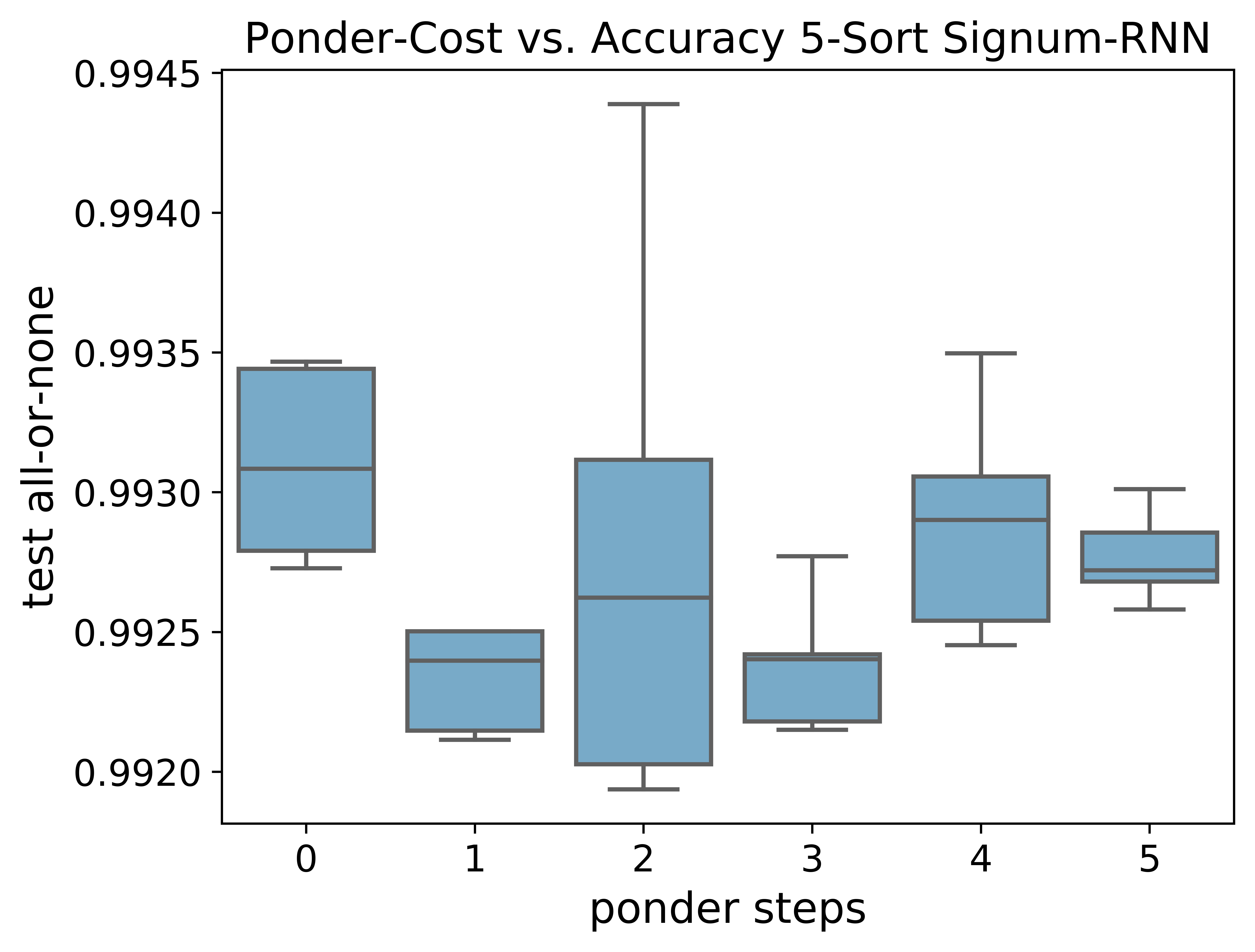
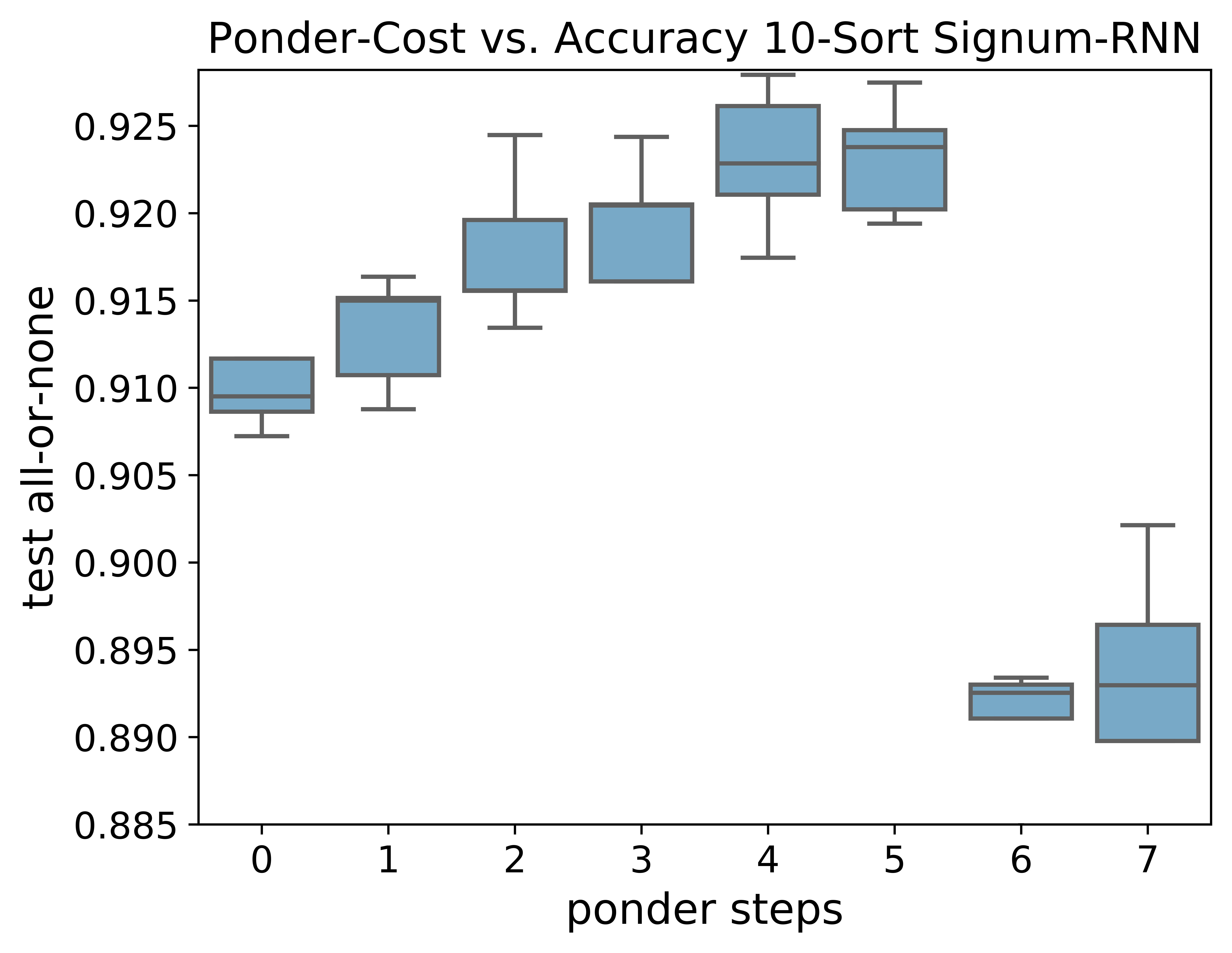
The model presented in [52] evaluates the effect of pondering in which they iterate an LSTM with no further inputs. This pondering allows the model to learn to sort its internal representation. Traditional sorting algorithms run $O(\log T)$ operations on the $T$ dimensional input sequence. Iterating the LSTM attempts to parallel this. We introduce a similar pondering loop into our model and show the performance benefit in Figure 4; we observe a similar performance gain, but notice that the benefits decrease after five pondering iterations.

Figure 5: We sweep a range of bits-per-pixel (BPP) values for FashionMNIST and CIFAR10, performing 5 experiments at each BPP level per model type (results reported as mean $\pm$ std). Left: Test Multi-Scale Structural Similarity (MS-SSIM) [54]. Middle: Purely unsupervised linear posterior test-classification accuracy. Right: Test input images and their reconstructions at BPP=0.1.

4.2 Unsupervised Discrete Representations

In this experiment, we study the usefulness of learnt unsupervised representations by latent variable models such as the Variational Autoencoder (VAE) [30]. Variational Autoencoders, coupled with Gumbel relaxed reparameterization methods [37, 26] enable learning of compact binary latent representations. Given an input random variable $x\sim p(x)$, VAEs posit an approximate posterior, $q_{\phi}(z_{2}|x)$, over a latent variable, $z_{2}$, and maximize the Evidence Lower BOund (ELBO). We contrast the VAE ELBO with our optimization objective below :

VAE: $\!\begin{aligned} \mathbb{E}_{q}[\log p_{\theta}(x|z_{2})]-D_{KL}[q_{\phi}(z_{2}|x)||p(z)]\end{aligned}$

DAB: $\!\begin{aligned} \mathbb{E}_{q}[\log p_{\theta}(x|z_{\text{hard}})]+\mathbb{E}_{q}[\gamma\log q(z_{\text{hard}}|l_{\phi}(z_{1}))]\end{aligned}$

In the case of the DAB model, $q(z_{\text{hard}}|l_{\phi}(z_{1}))\sim\mathcal{N}(l_{\phi}(z_{1}),I)$. This formulation is equivalent to the one from Section 3 since the log-likelihood of a Gaussian distribution (evaluated on a sample $z_{\text{hard}}$) is proportional to the L2-loss (Appendix Section 6.5.1). The specific functional value of $z_{\text{hard}}$ is based on the type of non-differential function used and is listed in Table 2.

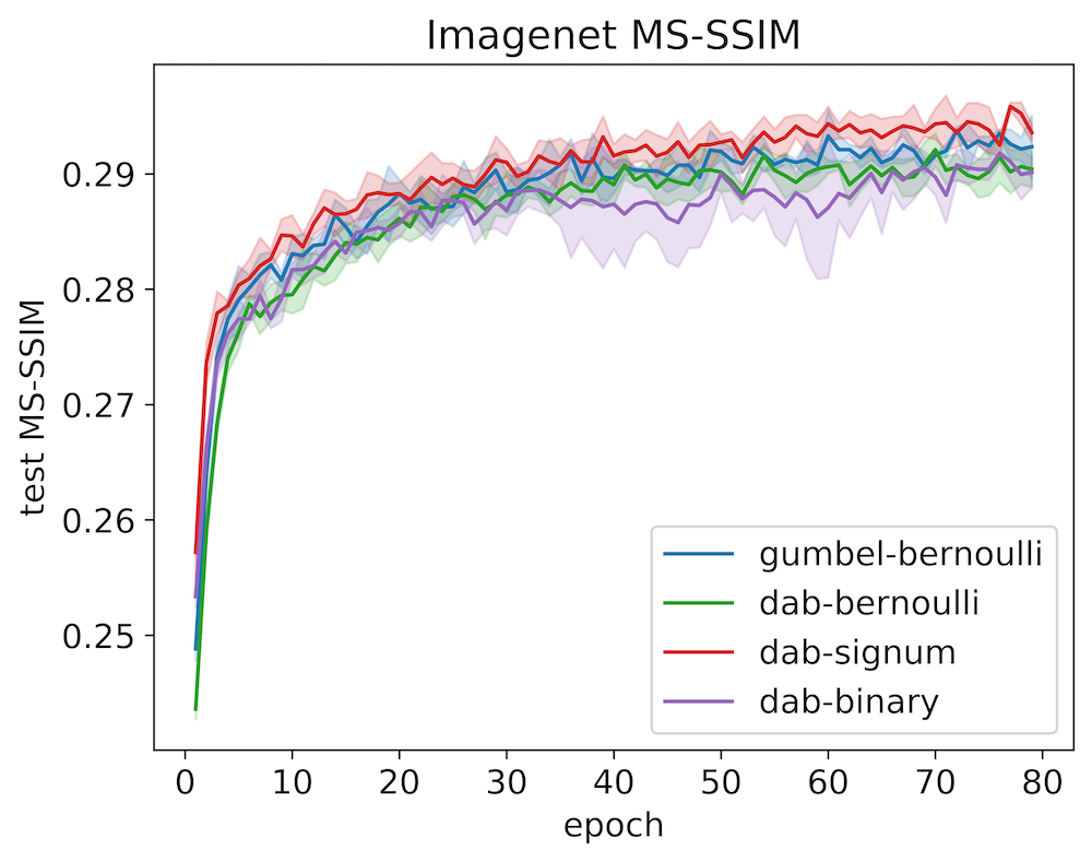
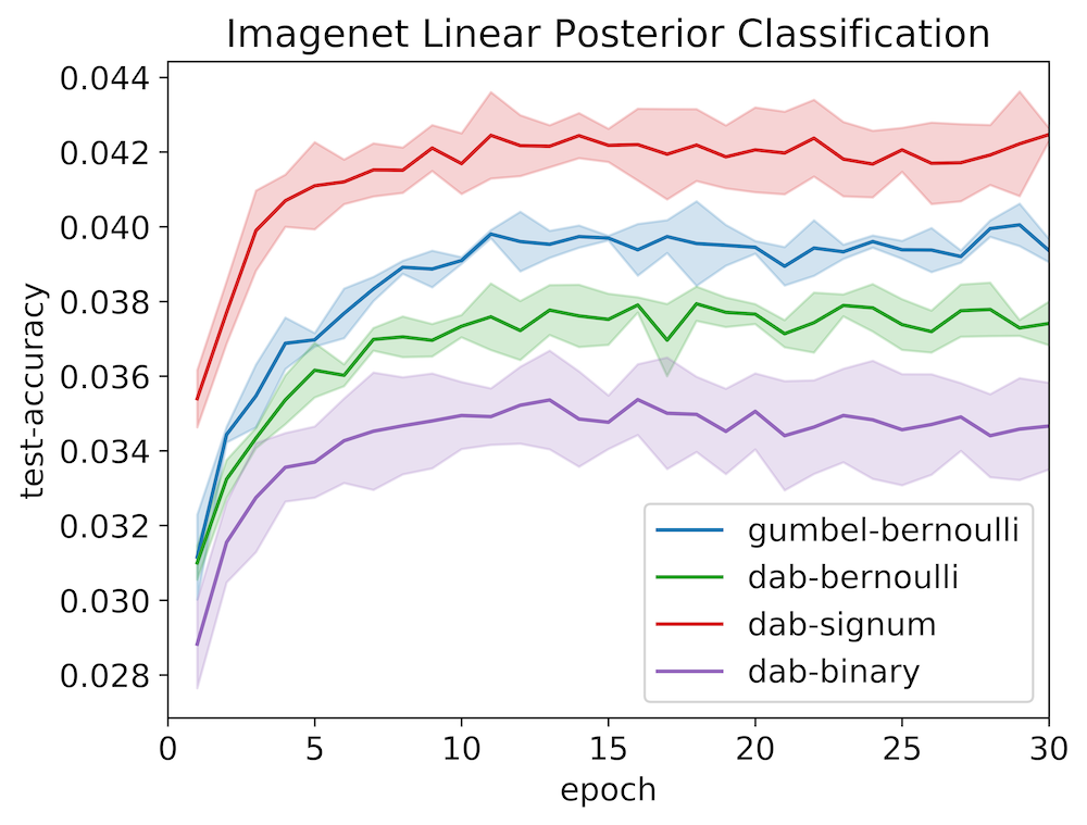
Good latent representions should not only be compact (in terms of bits-per-pixel), but also useful as a mechanism to produce a more separable representation space, $z_{2}$. In addition, given a latent representation the model should be able to reconstruct the original sample well. We demonstrate the usefulness of non-differentiable functions to both these objectives through the use of two metrics: the MS-SSIM [54] and linear classification of posterior samples. The MS-SSIM is a metric that provides a sense of how similar (in structure) the reconstructed image is to the original. Linear classification of posterior samples provides us with an evaluation of separable latent representations: a useful property for models that use the latent representation in downstream tasks. Importantly, we do not specifically train the model to induce better linearly separability as that would necessitate the use of supervision.

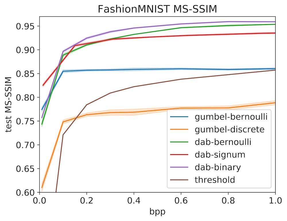
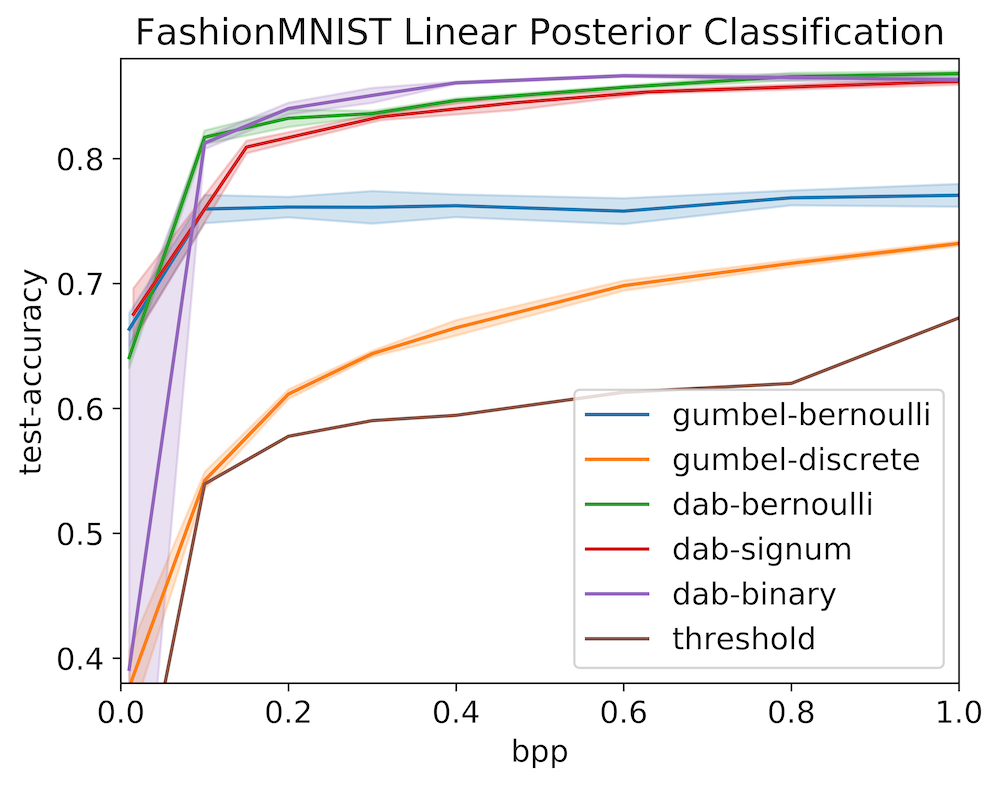
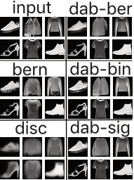
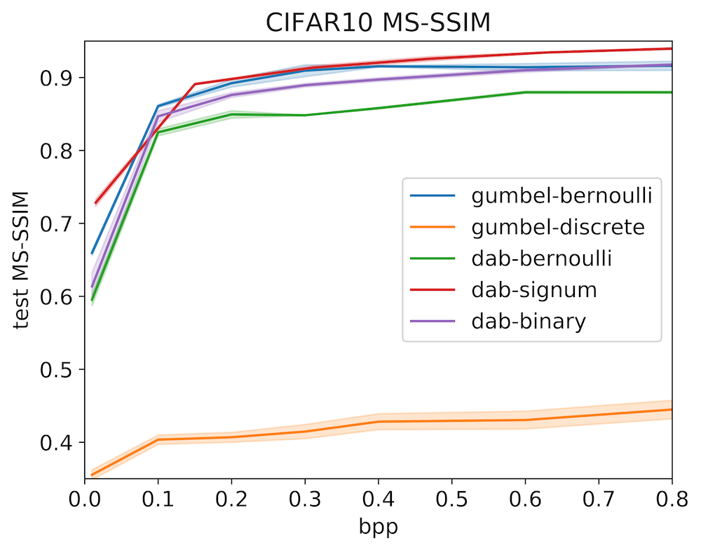
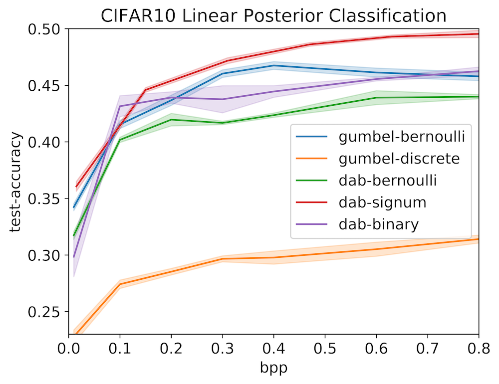
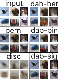
In Figure 5 and Table 3, we contrast our models (dab-*) against state of the art bernoulli and discrete relaxed gumbel-reparameterized models [37, 26] and a naive downsample, binary-threshold and classify using optimal threshold solution (threshold). The variants are summarized in Table 2 below:

	Functional Form
dab-bernoulli	Sample from non-reparameterized distribution: $z_{\text{hard}}\sim Bern(l_{\theta_{1}}(x))$.
dab-binary	$\!\begin{aligned} bin(z_{1})&=\begin{cases}1&z_{1}\geq\text{mean}(z_{1})\\ 0&z_{1}<\text{mean}(z_{1})\end{cases}\end{aligned}$
dab-signum	Equation 1. BPP is scaled by $\log_{2}(3)$ due to trinary representation.
threshold	bilinear(x, BPP), threshold(x, $\tau$) and linearly classify for the best $\tau$.

Table 2: Variants of activations used in experiment.

We begin by using the training set of Fashion MNIST, CIFAR10, and ImageNet to train the baseline bernoulli and discrete VAEs as well as the models with the non-differentiable functions (dab-*) presented above. We train five models per level of bpp for FashionMNIST and CIFAR10 and evaluate the MS-SSIM and linear classification accuracy at each point. We repeat the same, but only for bpp=0.00097 for Imagenet ($512\times 512\times 3$) due to computational restrictions. Each epoch of training at this resolution takes approximately 1.5 hours on 8 V-100 GPUs. Note that bpp=0.00097 requires a matrix that projects into a 786 dimensional space. Increasing this dimension substantially increases the parameters of the network. The linear classifier is trained on the same training dataset after the completion of training of the generative model. We present the mean and standard deviation results in Figure 5 and Table 3 for all three datasets.

Imagenet BPP = 0.00097 (768 dimensional latent) MS-SSIM Linear Separability Gumbel-Bernoulli 0.295 +/- 0.00058 0.0405 +/- 0.00035 DAB-Signum $\dagger$ 0.296 +/- 0.00063 0.0430 +/- 0.00068 DAB-Bernoulli 0.293 +/- 0.00051 0.0387 +/- 0.00022 DAB-Binary 0.292 +/- 0.00062 0.0356 +/- 0.00092

Table 3: Five trials (each) of ImageNet using only BPP=0.00097 (results reported as mean $\pm$ std). Images are compressed from $\mathbb{R}^{512\times 512\times 3}$ to 786 bits ($\dagger$ 496 for dab-signum since $786\approx 496\log_{2}3$) and yield a 43x improvement over random guessing (0.001). Full test curves in Appendix Section 6.3.

We observe that our models perform better in terms of test-reconstruction (MS-SSIM) and also provide a more separable latent representation (in terms of linear test accuracy). We observe either dab-signum or dab-binary performing better than all variants across all datasets. Since only the activation is being changed, the benefit can be directly attributed to the use of the non-differentiable functions used as activations. Since the DAB-decoder only operates over discrete inputs, it drastically simplifies the learning problem for this network. This contrasts the Gumbel-Softmax estimator which slowly anneals a continuous distribution to a discrete one over the training process. This validates the core tenant of DAB: use discrete (non-differentiable) outputs during the forward functional evaluations, but provide a smooth K-Lipschitz gradient during backpropagation.

4.2.1 Contrasting State of the Art Discrete Estimators

In order to relate this work to newer state of the art discrete estimators [49, 16], we parallel the simple VAE experiments used for RELAX [16] and REBAR [49]. The experiment proposed in [49, 16] is to estimate a (variational) density model for Binarized MNIST and Binarized Omniglot using a latent variable posterior distribution of 200 Bernouilli random variables. This task is challenging for neural networks that learn with gradient descent, as quantization (of the forward functional evaluations) removes the subtle directional information from the gradients. Thus, all of the proposed relaxed estimators [37, 26, 49, 16] use some form of annealed continuous distribution (such as the Gumbel distribution) during their forward functional evaluations. These distributions provide the model with continuous gradient information to update parameters during backpropagation. Over time, these continuous distributions are annealed towards the desired discrete representation, albeit sometimes with large variance [49]. In contrast, DABs always use discrete outputs during forward functional evaluations, while providing a smooth, K-Lipschitz gradient to enable learning. This approach allows the decoder in the VAE model to restrict itself to the range of discrete numerical values that the problem specifies.

As in [49, 16], we use a single hidden layer model with ReLU activations and 200 latent Bernouilli random variables. Adam is used as an optimizer with a learning rate of 3e-4 and $\gamma$ from Equation 2 is fixed to 10. In contrast to Experiment 4.2, we optimize the following objective:

$$\begin{split}\textbf{DAB-VAE}:\mathbb{E}_{q}[\log p_{\theta}(x|z_{\text{hard}})]-D_{KL}[q_{\phi}(l_{\phi}(z_{1})|x)||p(z)]\\ +\mathbb{E}_{q}[\gamma\log q(z_{\text{hard}}|l_{\phi}(z_{1}))]\end{split}$$ (3)

The objective in Equation 3 ensures that the the DAB-VAE compress the latent variable in a manner similar to REBAR and RELAX.

CIFAR10 Test-Accuracy	Mean	+/- Std	Functional Form
Baseline	92.87%	0.06%	Identity($z_{1}$)
Signum	91.95%	0.07%	Equation 1
Sort	92.93%	0.1%	sort-row($z_{1}$) $\oplus$ sort-col($z_{1}$)
Topk	92.21%	0.14%	(sort-row($z_{1}$) $\oplus$ sort-col($z_{1}$))[0:k]
K-Means	91.97%	0.16%	kmeans($z_{1}$, k=10)

Table 4: CIFAR10 test-accuracy over five trials for each row. $\oplus$ is a concatenation.

Binarized MNIST Binarized Omniglot Epochs Binarized MNIST Epochs Binarized Omniglot REBAR [49] -111.12 -127.51 331 368 RELAX [16] -119.19 -128.20 --- --- DAB (ours) -109.59 -125.19 9933 2366

Table 5: Binarized MNIST & Omniglot test variational lower bound (ELBO) in nats and training epochs to convergence. --- indicates non-reported values.

We report the best test variational lower bound (Equation 3 without $\mathbb{E}_{q}[\gamma\log q(z_{\text{hard}}|l_{\phi}(z_{1}))]$ to provide a meaningful comparison) for Binarized MNIST and Omniglot in Table 5 (larger ELBO values being better) . The same table also provides the number of training epochs needed for each model to converge to their reported best value. While DAB takes longer to converge, both REBAR and RELAX begin to overfit and continued training does not improve the bound. We observed that the generalization gap for DAB (1-2 nats) was smaller than RELAX and REBAR (5-10 nats). This improvement is because the decoder, $\log p_{\theta}(x|z_{\text{hard}})$, is required to reconstruct (at training and testing) the input sample, $x$, using a latent variable sampled from a stochastic, non-differentiable function, $z_{\text{hard}}\sim Bern(l_{\theta_{1}}(x))$. DAB outperforms both REBAR and RELAX on both the Binarized Omniglot and Binarized MNIST problems; the relative simplicity of training makes it a strong candidate for applications requiring non-differentiable functions. Adding a learning rate scheduler to the DAB based training is likely to improve convergence time, however this is left to future work.

4.3 Image Classification

Figure 6: Left: Signum non-differentiable function evaluated at different sections of a Resnet18 model. Middle: Earth mover distance between input to non-differentiable function and output of non-differentiable function. Right: CIFAR10 test accuracy for DAB vs. Straight-Through-Estimator using Sort-1D.

This experiment evaluates how well a DAB enhanced model performs in classifying images of CIFAR10 using a Resnet18 model tailored to operate on $\mathbb{R}^{32\times 32\times 3}$ images. We evaluate a variety of non-differentiable functions and present their test accuracy and standard deviation in Table 4. We observe that utilizing a sort as the final activation in the Resnet18 model improves upon the vanilla model (Baseline) by 0.1%. While these results show that DAB outperforms the baseline Resnet18 model, the difference is small. In contrast, when we used the same non-differentiable function in a simpler multi-layer dense model for the same problem, we observed a larger difference ($\approx$10%) between the test-accuracies. We attribute this to the quantization based regularization effect induced by the choice of non-differentiable activation.

Many of the tested non-differentiable activations in Table 4 perform equivalently to the state of the art (Baseline). DAB enables the exploration of novel networks with unconvential layers, including ones (such as MergeSort) which generalize to arbitrary numerical values. These unconvential activations can also be used for auxiliary tasks (eg: [50]).

4.3.1 Classification Ablation / Case Studies

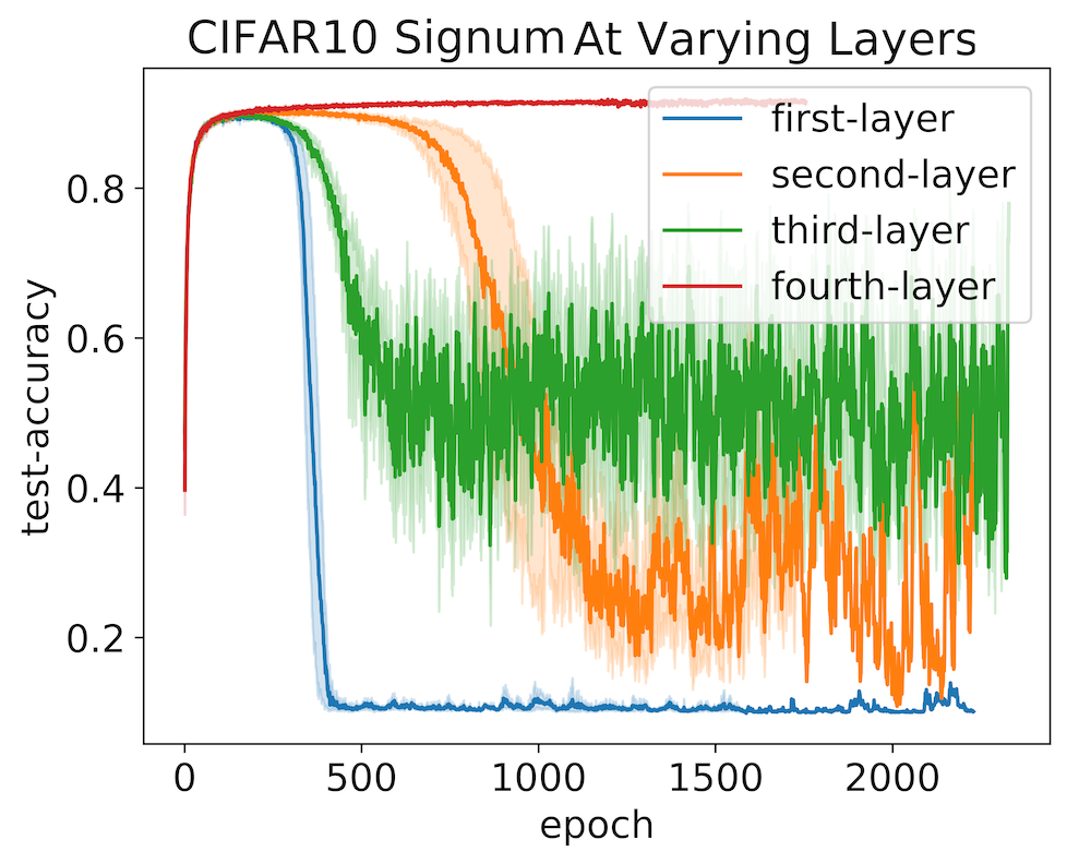
Layer Placement: In order to validate where to place the non-differentiable function within the Resnet18 architecture, we perform an ablation study. Since the Resnet18 model has four residual blocks, we place the non-differentiable function at the output of each block and train with each configuration 5 times (Figure 6-left). We observe that the network remains stable throughout training when the non-differentiable function is after he fourth layer and use this configuration for all experiments presented in Table 4.

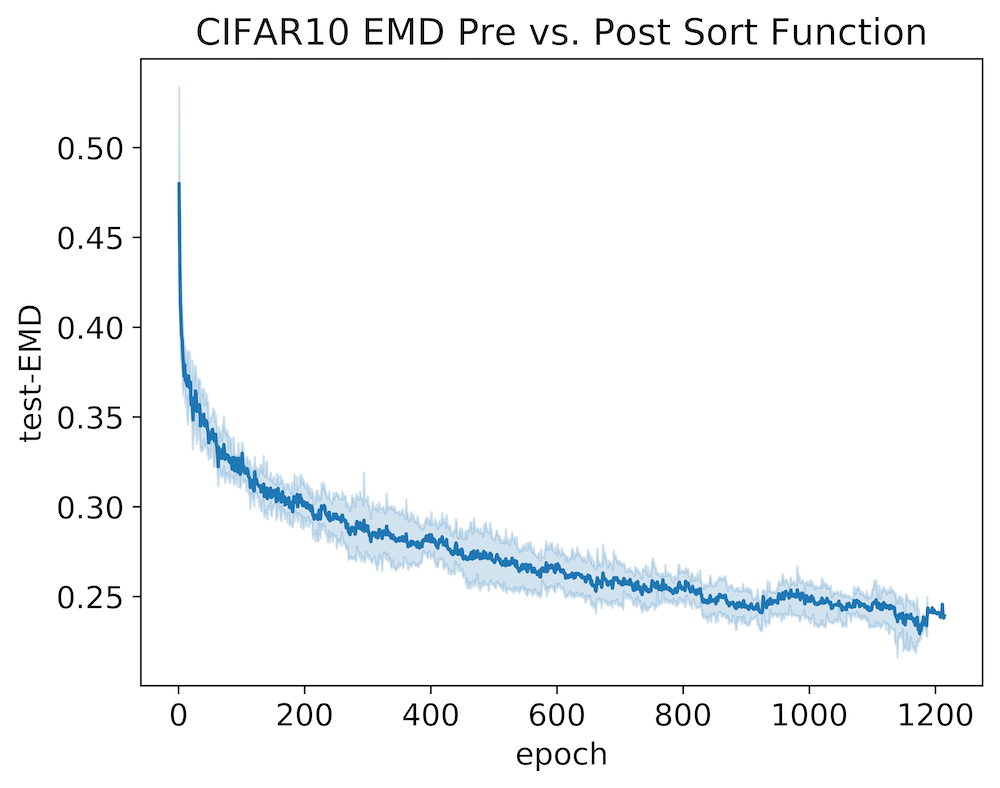
Conditioning of Preceding Layer: We utilize the Sort non-differentiable function shown in Table 4 to explore the effect of the regularizer introduced in Equation 2. We calculate the empirical earth mover distance between the input to the non-differentiable function ($z_{1}$ in Figure 2) and its output ($z_{\text{hard}}$ in Figure 2). We repeat the experiment five times and report the mean and standard deviation in Figure 6-middle. The regularizer conditions the input layer to produce partially sorted values, as demonstrated by the decrease in the test EMD over time.

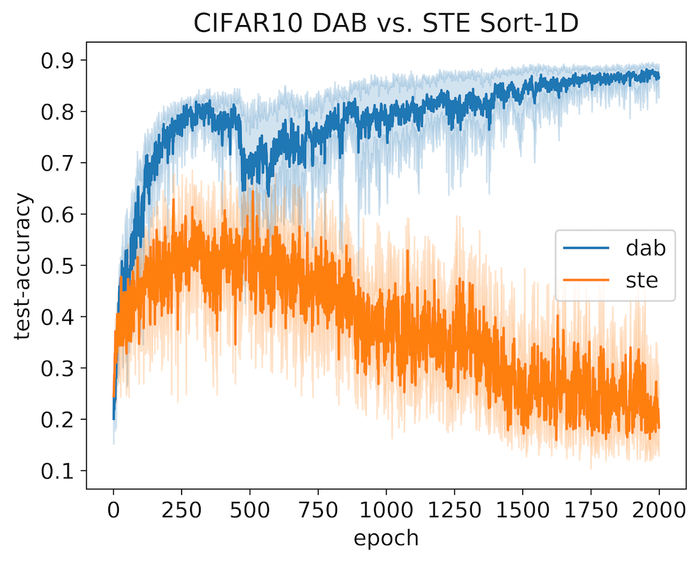
Contrasting the STE: The straight-through-estimator (STE) was originally used to bypass differentiating through a simple argmax operator [5], however, here we analyze how well it performs when handling a complex operand such as sorting. Since the STE cannot operate over transformations that vary in dimensionality, we use a simplified version of the sort operator from the previous experiment. Instead of sorting the rows and columns as in Table 4, we simply flatten the feature map and run a single sort operation. This allows us to use the STE in this scenario. We observe in Figure 6-right that DAB clearly outperforms the STE.

5 Discussion

Extensive research in machine learning has focused on discovering new (sub-)differentiable non-linearities to use within neural networks [20, 31, 41]. In this work, we demonstrate a novel method to allow for the incorporation of simple non-differentiable functions within neural networks and empirically demonstrate their benefit through a variety of experiments using a handful of non-differentiable operators, such as kmeans, sort, and signum. Rather than manually deriving sub-differentiable solutions (eg: [18]), using the Straight-Through-Estimator (eg: [50]) or relying on REINFORCE, we train using a neural network to learn a smooth approximation to the non-differentiable function. This work opens up the use of more complex non-differentiable operators within neural network pipelines.

6 Appendix

6.1 Simple Pytorch Implementation

We provide an example of the base class for any hard function along with an example of the $\epsilon$-margin signum operand (Equation 1) below. The BaseHardFn accepts the input tensor x along with the DAB approximation (soft_y). Coupling this with the DAB loss (Equation 6.5.1) provides a basic interface for using DABs with any model.

⬇

@staticmethod

def forward(ctx, x, soft_y, hard_fn, *args):

””” Runs the hard function for forward, cache the output and returns.

All hard functions should inherit from this, it implements the autograd override.

:param ctx: pytorch context, automatically passed in.

:param x: input tensor.

:param soft_y: forward pass output (logits) of DAB approximator network.

:param hard_fn: to be passed in from derived class.

:param args: list of args to pass to hard function.

:returns: hard_fn(tensor), backward pass using DAB.

:rtype: torch.Tensor

”””

hard = hard_fn(x, *args)

saveable_args = list([a for a in args if isinstance(a, torch.Tensor)])

ctx.save_for_backward(x, soft_y, *saveable_args)

return hard

@staticmethod

def _hard_fn(x, *args):

raise NotImplementedError(”implement _hard_fn in derived class”)

@staticmethod

def backward(ctx, grad_out):

””” Returns DAB derivative.

:param ctx: pytorch context, automatically passed in.

:param grad_out: grads coming into layer

:returns: dab_grad(tensor)

:rtype: torch.Tensor

”””

x, soft_y, *args = ctx.saved_tensors

with torch.enable_grad():

grad = torch.autograd.grad(outputs=soft_y, inputs=x,

grad_outputs=grad_out,

retain_graph=True)

return grad[0], None, None, None

class SignumWithMargin(BaseHardFn):

@staticmethod

def _hard_fn(x, *args):

””” x[x < -eps] = -1

x[x > +eps] = 1

else x = 0

:param x: input tensor

:param args: list of args with 0th element being eps

:returns: signum(tensor)

:rtype: torch.Tensor

”””

eps = args[0] if len(args) > 0 else 0.5

sig = torch.zeros_like(x)

sig[x < -eps] = -1

sig[x > eps] = 1

return sig

@staticmethod

def forward(ctx, x, soft_y, *args):

return BaseHardFn.forward(ctx, x, soft_y, SignumWithMargin._hard_fn, *args)

6.2 Contrasting RELAX and REBAR

Figure 7: Test Negative Variational Lower Bound (-ELBO) [lower being better]. Left: Binarized MNIST. Right: Omniglot.

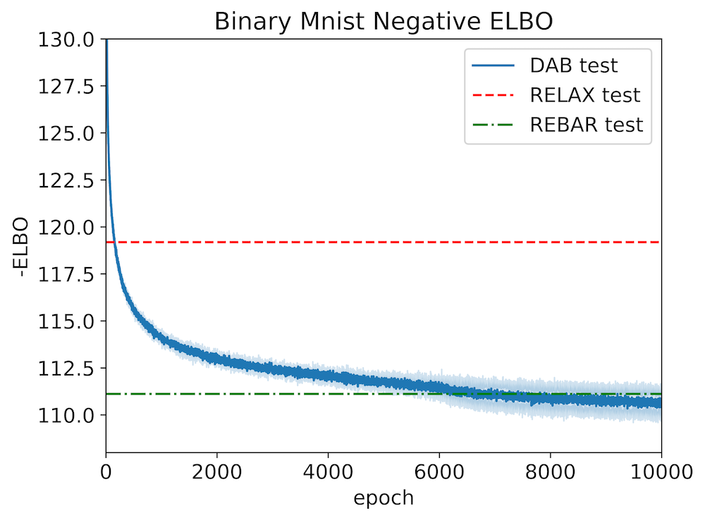
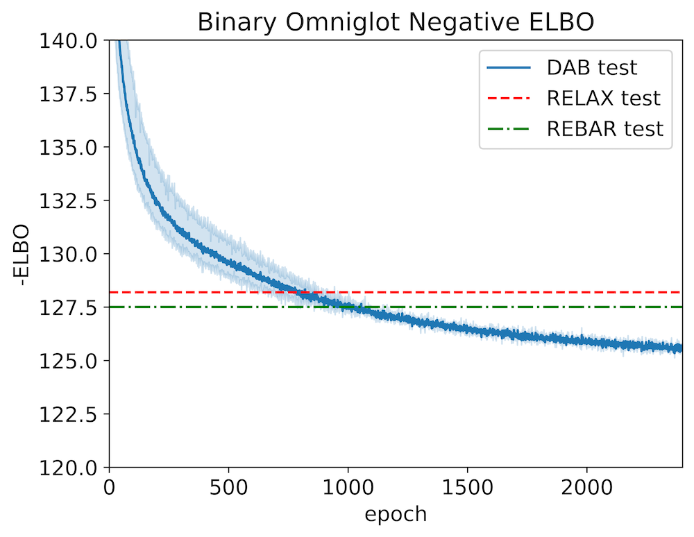
While REBAR and RELAX used learning rate schedulers, we used a fixed learning rate of 3e-4 with Adam for the entirety of training. We believe that using a scheduled learning rate will improve time to convergence for DAB, but leave this for future work.

6.3 Imagenet Test Curves for MS-SSIM and Linear Separability

The full test curves for Imagenet are shown below:

Figure 8: Five trials (each) of ImageNet using only BPP=0.00097 due to computational restrictions (results reported as mean $\pm$ std). Left: Test MS-SSIM [54]. Right: Purely unsupervised linear posterior test-classification accuracy; Images are compressed from $\mathbb{R}^{512\times 512}$ to 786 bits (496 for dab-signum since $786\approx 496\log_{2}(3)$) and yield a 40x improvement over random guessing (0.001).

6.4 Model Hyper-Parameters

	FashionMNIST	CIFAR10	ImageNet	Sorting	Classification
Optimizer	Adam	RMSProp	RMSProp	Adam	Adam
LR	1e-3	1e-4	1e-4	1e-4	1e-4
Batch-Size	128	128	192	1024	128
Activation	ELU	ReLU	ELU	Tanh	ELU
Normalization	Batchnorm	Batchnorm-Conv, None-Dense	Batchnorm-Conv, None-Dense	None	Batchnorm
Layer-Type	Similar to U-Net	Coord-Conv encoder, Dense decoder	Resnet18 encoder, Dense decoder	LSTM (gradclip 5) + Dense(256)	CifarResnet18
DAB-$\gamma$	10	70	2	10	10

6.5 Bayesian Interpretation of DAB

Figure 9: Graphical model of our proposed framework. $\color[rgb]{1,0,0}\definecolor[named]{pgfstrokecolor}{rgb}{1,0,0}l_{hard}$ represents the non-differentiable function and $\color[rgb]{1,0,0}\definecolor[named]{pgfstrokecolor}{rgb}{1,0,0}z_{hard}$ its (latent variable) outputs.

A graphical model depicting a generic version of our framework is shown in Figure 2. Given some true input data distribution, $x\sim p(x),y\sim p(y|x)$, and a set of $J$ ($J=3$ in Figure 9) functional approximators, $l_{\theta_{i}}:\mathbb{R}^{N}\mapsto\mathbb{R}^{N},\ i\in\{1..J\}$, our learning objective is defined as maximizing the log likelihood, $\log p_{\theta}(y|x)$, coupled with a new regularizer, $\log p_{\phi}(z_{\text{hard}}|z_{\phi})$ ($\mathcal{L}_{DAB}$ in Figure 9), introduced in this work:

$$\max_{\theta,\phi}\ \mathcal{J}(\theta,\phi)=\mathbb{E}_{x}[\ \log p_{\theta}(y|x)+\gamma\ \log p_{\phi}(z_{\text{hard}}|z_{\phi})\ ],$$ (4)

$$=\mathbb{E}_{x}[\ \log p_{\theta}(y|z_{\text{hard}})\ p_{\phi}(z_{\text{hard}}|z_{1})\ p_{\theta}(z_{1}|x)+\gamma\ \log p_{\phi}(z_{\text{hard}}|z_{\phi})\ ],$$ (5)

$$=\mathbb{E}_{x}[\ \log p_{\theta}(y|l_{\theta_{3}}({\color[rgb]{1,0,0}\definecolor[named]{pgfstrokecolor}{rgb}{1,0,0}l_{\text{hard}}}(l_{\theta_{1}}(x))))+\gamma\ \log p_{\phi}(z_{\text{hard}}|l_{\phi}(z_{1}))\ ].$$ (6)

We transition from Equation 4 to Equation 5 by using the conditional independence assumptions from our graphical model in Figure 9. Since the latent representations $z_{i}$ are simple functional transformations, we can represent the distributions $,p(z_{i}|z_{i-1}),\ i>0$ (Equation 5), by dirac distributions centered around their functional evaluations: $z_{i}|z_{i-1}\sim\delta(l_{\theta_{i}}(z_{i-1}))$. This allows us to rewrite our objective as shown in Equation 6, where $\gamma$ is a problem specific hyper-parameter. A key point is that during the forward functional evaluations of the model we use the non-differentiable function, ${\color[rgb]{1,0,0}\definecolor[named]{pgfstrokecolor}{rgb}{1,0,0}l_{\text{hard}}}$.

Note that we have kept our framework generic. In the following section we will describe the gaussianity assumptions on the regularizer $p_{\phi}(z_{\text{hard}}|z_{1})$ and why it converges.

6.5.1 Choice of metric under simplifying assumptions

In this section we analyze the regularizer introduced in Equation 6 / Equation 2 in the special case where the non-differentiable function output, $z_{\text{hard}}={\color[rgb]{1,0,0}\definecolor[named]{pgfstrokecolor}{rgb}{1,0,0}l_{\text{hard}}}(z_{1})=\phi z_{1}+\epsilon$, is a (differentiable) linear transformation of the previous layer coupled with additive Gaussian noise (aleatoric uncertainty):

$$z_{\text{hard}} =\phi z_{1}+\epsilon,\ \epsilon\sim\mathcal{N}(0,\sigma^{2}),$$ (7)

$$z_{\text{hard}}|\phi z_{1},\sigma^{2} \sim\prod_{i=1}^{N}\mathcal{N}(\phi z_{1},\sigma^{2}).$$ (8)

Under these simplifying assumptions our model induces a Gaussian log-likelihood as shown in Equation 8. At this point we can directly maximize the above likelihood using maximum likelihood estimation. Alternatively, if we have apriori knowledge we can introduce it as a prior, $p(\phi)$, over the weights $\phi$, and minimize the negative log-likelihood multiplied by the prior to evaluate the posterior (which will be induced as a gaussian), i.e. the MAP estimate. If we make a conjugate prior assumption, $p(\phi)\sim\mathcal{N}(0,\sigma^{2}_{\phi})$, then:

$$-\log(\text{posterior}) \propto-\log\prod_{i=1}^{N}\underbrace{\mathcal{N}(\phi z_{1},\sigma^{2})}_{\text{likelihood}}\underbrace{\mathcal{N}(0,\sigma^{2}_{\phi})}_{\text{prior}},$$ (9)

$$=\sum_{i=1}^{N}\frac{-1}{\sigma^{2}}(z_{\text{hard}}-\phi z_{1})^{2}-\frac{\phi^{2}}{\sigma_{\phi}^{2}}+\text{const},$$ (10)

$$\propto||z_{\text{hard}}-\phi z_{1}||_{2}^{2}.$$ (11)

This analysis leads us to the well known result that a linear transformation with aleatoric Gaussian noise results in a loss proportional to the L2 loss (Equation 11). However, what can we say about the case where $z_{\text{hard}}$ is a non-linear, non-differentiable output? In practice we observe that using the L2 loss, coupled with a non-linear neural network transformation, $l_{\phi}(z_{1})$ produces strong results. To understand why, we appeal to the central limit theorem which states that the scaled mean of the random variable converges to a Gaussian distribution as the sample size increases. Furthermore, if we can assume a zero mean, positive variance, and finite absolute third moment, it can be shown that the rate of convergence to a Gaussian distribution is proportional to $\frac{1}{\sqrt{N}}$, where $N$ is the number of samples [6].

Sketch of Convergence Proof:

Given: the true distribution converges to a Gaussian (in the limit) as per Section 6.5.1.

Given: neural networks are universal function approximators [22],

then in the limit, $l_{\phi}(z_{1})\approx l_{\text{hard}}(z_{1})$ which implies $\frac{\delta l_{\phi}}{\delta l_{\theta_{1}}}\approx\frac{\delta l_{\text{hard}}}{\delta l_{\theta_{1}}}$.

Then DAB converges via the least-squares estimator to the true distribution via the least-square estimator

convergence proofs of [33, 34, 19, 7].

We empirically explored alternatives such as the Huber loss [23], cosine loss, L1 loss and cross-entropy loss, but found the L2 loss to consistently produce strong results and we use it for all presented experiments.

References

- [1] A. F. Agarap. Deep learning using rectified linear units (relu). arXiv preprint arXiv:1803.08375, 2018.
- [2] T. Asselmeyer, W. Ebeling, and H. Rosé. Evolutionary strategies of optimization. Physical Review E, 56(1):1171, 1997.
- [3] K. E. Batcher. Sorting networks and their applications. In Proceedings of the April 30–May 2, 1968, spring joint computer conference, pages 307–314. ACM, 1968.
- [4] E. Belilovsky, M. Eickenberg, and E. Oyallon. Decoupled greedy learning of cnns. arXiv preprint arXiv:1901.08164, 2019.
- [5] Y. Bengio, N. Léonard, and A. Courville. Estimating or propagating gradients through stochastic neurons for conditional computation. arXiv preprint arXiv:1308.3432, 2013.
- [6] A. C. Berry. The accuracy of the gaussian approximation to the sum of independent variates. Transactions of the american mathematical society, 49(1):122–136, 1941.
- [7] S. Bittanti and M. CAMP. Recursive least-squares identification algorithms with incomplete excitation: Convergence analysis and application to adaptive control. IEEE Transactions on Automatic Control, 35(12), 1990.
- [8] D. Brodsky and B. Watson. Model simplification through refinement. In Graphics Interface, volume 2000, pages 221–228. Citeseer, 2000.
- [9] J. Devlin, M.-W. Chang, K. Lee, and K. Toutanova. Bert: Pre-training of deep bidirectional transformers for language understanding. In Proceedings of the 2019 Conference of the North American Chapter of the Association for Computational Linguistics: Human Language Technologies, Volume 1 (Long and Short Papers), pages 4171–4186, 2019.
- [10] A. E. Gelfand and A. F. Smith. Sampling-based approaches to calculating marginal densities. Journal of the American statistical association, 85(410):398–409, 1990.
- [11] W. R. Gilks, S. Richardson, and D. Spiegelhalter. Markov chain Monte Carlo in practice. Chapman and Hall/CRC, 1995.
- [12] P. Glasserman. Monte Carlo methods in financial engineering, volume 53. Springer Science & Business Media, 2013.
- [13] P. W. Glynn. Likelihood ratio gradient estimation for stochastic systems. Communications of the ACM, 33(10):75–84, 1990.
- [14] D. E. Goldberg and J. H. Holland. Genetic algorithms and machine learning. Machine learning, 3(2):95–99, 1988.
- [15] I. Goodfellow, J. Pouget-Abadie, M. Mirza, B. Xu, D. Warde-Farley, S. Ozair, A. Courville, and Y. Bengio. Generative adversarial nets. In Advances in neural information processing systems, pages 2672–2680, 2014.
- [16] W. Grathwohl, D. Choi, Y. Wu, G. Roeder, and D. Duvenaud. Backpropagation through the void: Optimizing control variates for black-box gradient estimation. ICLR, 2018.
- [17] R. Gray. Vector quantization. IEEE Assp Magazine, 1(2):4–29, 1984.
- [18] E. Grefenstette, K. M. Hermann, M. Suleyman, and P. Blunsom. Learning to transduce with unbounded memory. In Advances in neural information processing systems, pages 1828–1836, 2015.
- [19] L. Guo. Self-convergence of weighted least-squares with applications to stochastic adaptive control. IEEE transactions on automatic control, 41(1):79–89, 1996.
- [20] R. H. Hahnloser, R. Sarpeshkar, M. A. Mahowald, R. J. Douglas, and H. S. Seung. Digital selection and analogue amplification coexist in a cortex-inspired silicon circuit. Nature, 405(6789):947, 2000.
- [21] K. He, X. Zhang, S. Ren, and J. Sun. Deep residual learning for image recognition. In Proceedings of the IEEE Conference on Computer Vision and Pattern Recognition, pages 770–778, 2016.
- [22] K. Hornik, M. Stinchcombe, and H. White. Multilayer feedforward networks are universal approximators. Neural networks, 2(5):359–366, 1989.
- [23] P. J. Huber. Robust estimation of a location parameter. In Breakthroughs in statistics, pages 492–518. Springer, 1992.
- [24] Z. Huo, B. Gu, and H. Huang. Training neural networks using features replay. In Advances in Neural Information Processing Systems, pages 6660–6669, 2018.
- [25] M. Jaderberg, W. M. Czarnecki, S. Osindero, O. Vinyals, A. Graves, D. Silver, and K. Kavukcuoglu. Decoupled neural interfaces using synthetic gradients. In Proceedings of the 34th International Conference on Machine Learning-Volume 70, pages 1627–1635. JMLR. org, 2017.
- [26] E. Jang, S. Gu, and B. Poole. Categorical reparameterization with gumbel-softmax. ICLR, 2017.
- [27] J. Katajainen and J. L. Träff. A meticulous analysis of mergesort programs. In Italian Conference on Algorithms and Complexity, pages 217–228. Springer, 1997.
- [28] J. Kennedy. Particle swarm optimization. Encyclopedia of machine learning, pages 760–766, 2010.
- [29] D. P. Kingma and J. Ba. Adam: A method for stochastic optimization. In Proceedings of the 3rd International Conference on Learning Representations (ICLR), 2014.
- [30] D. P. Kingma and M. Welling. Auto-encoding variational bayes. ICLR, 2014.
- [31] G. Klambauer, T. Unterthiner, A. Mayr, and S. Hochreiter. Self-normalizing neural networks. In Advances in neural information processing systems, pages 971–980, 2017.
- [32] J. P. Kleijnen and R. Y. Rubinstein. Optimization and sensitivity analysis of computer simulation models by the score function method. European Journal of Operational Research, 88(3):413–427, 1996.
- [33] T. L. Lai, C. Z. Wei, et al. Least squares estimates in stochastic regression models with applications to identification and control of dynamic systems. The Annals of Statistics, 10(1):154–166, 1982.
- [34] T. L. Lai and Z. Ying. Recursive identification and adaptive prediction in linear stochastic systems. SIAM Journal on Control and Optimization, 29(5):1061–1090, 1991.
- [35] T. P. Lillicrap, D. Cownden, D. B. Tweed, and C. J. Akerman. Random synaptic feedback weights support error backpropagation for deep learning. Nature communications, 7:13276, 2016.
- [36] F. Locatello, S. Bauer, M. Lucic, S. Gelly, B. Schölkopf, and O. Bachem. Challenging common assumptions in the unsupervised learning of disentangled representations. ICLR, 2019.
- [37] C. J. Maddison, A. Mnih, and Y. W. Teh. The concrete distribution: A continuous relaxation of discrete random variables. ICLR, 2017.
- [38] T. Mikolov, K. Chen, G. Corrado, and J. Dean. Efficient estimation of word representations in vector space. arXiv preprint arXiv:1301.3781, 2013.
- [39] S. Mohamed, M. Rosca, M. Figurnov, and A. Mnih. Monte carlo gradient estimation in machine learning. CoRR, abs/1906.10652, 2019.
- [40] A. Paszke, S. Gross, S. Chintala, G. Chanan, E. Yang, Z. DeVito, Z. Lin, A. Desmaison, L. Antiga, and A. Lerer. Automatic differentiation in pytorch. In NIPS-W, 2017.
- [41] P. Ramachandran, B. Zoph, and Q. V. Le. Searching for activation functions. arXiv preprint arXiv:1710.05941, 2017.
- [42] J. Ramapuram and R. Webb. A new benchmark and progress toward improved weakly supervised learning. BMVC, 2018.
- [43] L. M. Rios and N. V. Sahinidis. Derivative-free optimization: a review of algorithms and comparison of software implementations. Journal of Global Optimization, 56(3):1247–1293, 2013.
- [44] H. Robbins and S. Monro. A stochastic approximation method. The annals of mathematical statistics, pages 400–407, 1951.
- [45] D. Silver, A. Huang, C. J. Maddison, A. Guez, L. Sifre, G. Van Den Driessche, J. Schrittwieser, I. Antonoglou, V. Panneershelvam, M. Lanctot, et al. Mastering the game of go with deep neural networks and tree search. nature, 529(7587):484, 2016.
- [46] C. Szegedy, S. Ioffe, V. Vanhoucke, and A. Alemi. Inception-v4, inception-resnet and the impact of residual connections on learning. arXiv preprint arXiv:1602.07261, 2016.
- [47] J. Tenenbaum. Building machines that learn and think like people. In Proceedings of the 17th International Conference on Autonomous Agents and MultiAgent Systems, pages 5–5. International Foundation for Autonomous Agents and Multiagent Systems, 2018.
- [48] A. Trask, F. Hill, S. E. Reed, J. Rae, C. Dyer, and P. Blunsom. Neural arithmetic logic units. In Advances in Neural Information Processing Systems, pages 8035–8044, 2018.
- [49] G. Tucker, A. Mnih, C. J. Maddison, J. Lawson, and J. Sohl-Dickstein. Rebar: Low-variance, unbiased gradient estimates for discrete latent variable models. In Advances in Neural Information Processing Systems, pages 2627–2636, 2017.
- [50] A. van den Oord, O. Vinyals, et al. Neural discrete representation learning. In Advances in Neural Information Processing Systems, pages 6306–6315, 2017.
- [51] P. J. Van Laarhoven and E. H. Aarts. Simulated annealing. In Simulated annealing: Theory and applications, pages 7–15. Springer, 1987.
- [52] O. Vinyals, S. Bengio, and M. Kudlur. Order matters: Sequence to sequence for sets. ICLR, 2016.
- [53] O. Vinyals, M. Fortunato, and N. Jaitly. Pointer networks. In Advances in Neural Information Processing Systems, pages 2692–2700, 2015.
- [54] Z. Wang, E. P. Simoncelli, and A. C. Bovik. Multiscale structural similarity for image quality assessment. In The Thrity-Seventh Asilomar Conference on Signals, Systems & Computers, 2003, volume 2, pages 1398–1402. Ieee, 2003.
- [55] C. J. Watkins and P. Dayan. Q-learning. Machine learning, 8(3-4):279–292, 1992.
- [56] R. J. Williams. Simple statistical gradient-following algorithms for connectionist reinforcement learning. Machine learning, 8(3-4):229–256, 1992.
- [57] H. Wu and X. Gu. Max-pooling dropout for regularization of convolutional neural networks. In International Conference on Neural Information Processing, pages 46–54. Springer, 2015.