Efficient and minimal length parametric conformal prediction regions

Daniel J. Eck1 and Forrest W. Crawford2,3,4,5
1. Department of Statistics, University of Illinois Urbana-Champaign
2. Department of Biostatistics, Yale School of Public Health
3. Department of Statistics & Data Science, Yale University
4. Department of Ecology & Evolutionary Biology, Yale University
5. Yale School of Management
Abstract

Conformal prediction methods construct prediction regions for iid data that are valid in finite samples. We provide two parametric conformal prediction regions that are applicable for a wide class of continuous statistical models. This class of statistical models includes generalized linear models (GLMs) with continuous outcomes. Our parametric conformal prediction regions possesses finite sample validity, even when the model is misspecified, and are asymptotically of minimal length when the model is correctly specified. The first parametric conformal prediction region is constructed through binning of the predictor space, guarantees finite-sample local validity and is asymptotically minimal at the log(n)/n𝑛𝑛\sqrt{\log(n)/n} rate when the dimension d𝑑d of the predictor space is one or two, and converges at the O{(log(n)/n)1/d}𝑂superscript𝑛𝑛1𝑑O\{(\log(n)/n)^{1/d}\} rate when d>2𝑑2d>2. The second parametric conformal prediction region is constructed by transforming the outcome variable to a common distribution via the probability integral transform, guarantees finite-sample marginal validity, and is asymptotically minimal at the log(n)/n𝑛𝑛\sqrt{\log(n)/n} rate. We develop a novel concentration inequality for maximum likelihood estimation that induces these convergence rates. We analyze prediction region coverage properties, large-sample efficiency, and robustness properties of four methods for constructing conformal prediction intervals for GLMs: fully nonparametric kernel-based conformal, residual based conformal, normalized residual based conformal, and parametric conformal which uses the assumed GLM density as a conformity measure. Extensive simulations compare these approaches to standard asymptotic prediction regions. The utility of the parametric conformal prediction region is demonstrated in an application to interval prediction of glycosylated hemoglobin levels, a blood measurement used to diagnose diabetes.
Keywords: conformity measure, maximum likelihood estimation, regression, generalized linear models, exponential families, finite sample validity, concentration inequalities

1 Introduction

Vovk et al. (2005) introduced conformal prediction to construct finite sample valid prediction regions for predictions from nearest-neighbor methods, support-vector machines, and sequential classification and both linear and ridge regression problems. The goal in conformal prediction is to construct a prediction region Cnsubscript𝐶𝑛C_{n} from an iid random sample Y1subscript𝑌1Y_{1}, \ldots, Ynsubscript𝑌𝑛Y_{n}, such that the probability of a future observation Yn+1subscript𝑌𝑛1Y_{n+1} belonging to the region Cnsubscript𝐶𝑛C_{n} exceeds a desired coverage level (Shafer and Vovk, 2008). That is, given Y1,,Ynsubscript𝑌1subscript𝑌𝑛Y_{1},\ldots,Y_{n}, we seek a set Cn=Cn(Y1,,Yn)subscript𝐶𝑛subscript𝐶𝑛subscript𝑌1subscript𝑌𝑛C_{n}=C_{n}(Y_{1},\ldots,Y_{n}) such that for 0<α<10𝛼10<\alpha<1,

(Yn+1Cn)1α.subscript𝑌𝑛1subscript𝐶𝑛1𝛼\mathbb{P}(Y_{n+1}\in C_{n})\geq 1-\alpha. (1)

Lei et al. (2013) extended the framework of Shafer and Vovk (2008) to provide a framework for which the prediction region Cnsubscript𝐶𝑛C_{n} is also asymptotically of minimal length. These prediction regions make use of a conformity measure σ𝜎\sigma which measures the agreement of a point y𝑦y with a probability measure P𝑃P. For example, when y𝑦y\in\mathbb{R}, the probability density function p𝑝p corresponding to P𝑃P is a conformity measure σ𝜎\sigma. Lei et al. (2013) proposed nonparametric kernel density estimation of p𝑝p to construct conformal prediction regions that are asymptotically minimal under smoothness conditions on p𝑝p. Beyond real-valued outcomes, conformal methods have been proposed for functional data (Lei et al., 2015), nonparametric regression (Lei and Wasserman, 2014), time series data (Chernozhukov et al., 2018b), high-dimensional regression problems (Lei et al., 2018), random effects (Dunn and Wasserman, 2018), causal inference (Chernozhukov et al., 2018a), machine learning (Vovk et al., 2005; Gammerman and Vovk, 2007; Papadopoulos et al., 2011; Vovk, 2012; Burnaev and Vovk, 2014; Balasubramanian et al., 2014; Johansson et al., 2018; Wang et al., 2018), and quantile regression (Romano et al., 2019a, b; Sesia and Candés, 2019). The finite sample validity property of conformal prediction regions has broad appeal in many scientific domains, including astrophysics (Ciollaro et al., 2018), medical applications (Lambrou et al., 2009; Devetyarov et al., 2012; Eklund et al., 2015; Bosc et al., 2019), genetics (Norinder et al., 2018b, a), and chemistry (Cortés-Ciriano and Bender, 2018; Ji et al., 2018; Svensson et al., 2018a, b; Toccaceli et al., 2017).

However, usefulness of the finite sample validity property of conformal prediction regions in regression may be offset by the size of the prediction region. Recently, Cortés-Ciriano and Bender (2019) stated that “a major issue in conformal prediction applied to regression is the low efficiency of most conformal prediction models…Such large intervals are not informative and thus hamper the practical usefulness of conformal prediction”, calling for the development of non-conformity functions to reduce the size of the predicted confidence regions (Cortés-Ciriano and Bender, 2019). The parametric conformal prediction regions that we develop in this paper answer the call made by Cortés-Ciriano and Bender (2019) in the context of regression. We show that when one uses the parametric density with maximum likelihood estimators (MLEs) of model parameters plugged in for modeling parameters as the conformity measure, then one can can construct conformal predictions that are asymptotically minimal length and our sharp under our proof technique. Our parametric conformal prediction regions possess the same finite-sample validity guarantees as existing conformal prediction procedures, even under model misspecification.

In a recent paper, Chernozhukov et al. (2019) proposed parametric conformal prediction regions based on regression models for conditional distributions, establishing the conditional validity of the resulting prediction intervals under consistent estimation of the conditional distributions. Their proposed prediction method is based on modeling the entire conditional distribution (rather than the conditional mean) and thereby generates conditionally valid prediction sets that fully utilize the information in the covariates (Chernozhukov et al., 2019). In another recent paper, Izbicki et al. (2019) proposed parametric conformal prediction regions that are asymptotically minimal length, without providing explicit convergence rates.

We build upon the frameworks outlined by Chernozhukov et al. (2019) and Izbicki et al. (2019) by providing two methods for constructing parametric conformal prediction regions which are asymptotically of minimal length with desirable rates of convergence. Both methods are constructed by using the maximum likelihood estimator as a plugin estimate of unknown modeling parameters in the underlying density and distribution functions. The first of these is conditionally valid in local regions of the predictor space (Lei and Wasserman, 2014, pg. 72), and is asymptotically conditionally valid for point predictions. The rate of convergence for this parametric conformal prediction region is O{log(n)/n}𝑂𝑛𝑛O\{\sqrt{\log(n)/n}\} when the dimension of predictor space is d2𝑑2d\leq 2 and is O{(log(n)/n)1/d}𝑂superscript𝑛𝑛1𝑑O\{(\log(n)/n)^{1/d}\} when d>2𝑑2d>2 where the predictor region of interest shrinks at a suitable rate. The construction of this conformal prediction region follows the binning technique in Lei and Wasserman (2014). The O{(log(n)/n)1/d}𝑂superscript𝑛𝑛1𝑑O\{(\log(n)/n)^{1/d}\} rate is a consequence of how quickly the predictor region of interest shrinks. The second parametric conformal prediction region is obtained by first transforming the outcome variable to a “common” distribution via the probability integral transform, and conducting conformal prediction with respect to this common distributions to obtain a finite sample marginally valid prediction region, and then backtransforming this region to the scale of the original outcome variables. We leverage the estimated density to obtain estimates of the quantiles corresponding to the minimal length (1α)×100%1𝛼percent100(1-\alpha)\times 100\% prediction region before we backtransform to the scale of the response. We show that this parametric conformal prediction region is asymptotically minimal at rate O{log(n)/n}𝑂𝑛𝑛O\{\sqrt{\log(n)/n}\}. The convergence rates for both parametric conformal regions are appreciably faster than that presented by Lei and Wasserman (2014) which gave rates of {log(n)/n}1/(d+3)superscript𝑛𝑛1𝑑3\left\{\log(n)/n\right\}^{1/(d+3)} for nonparametric conformal prediction regions in the same regression context.

Chernozhukov et al. (2019) developed a similar transformation conformal prediction region that is motivated by the probability integral transform. Their conformal prediction technique is based on the α/2𝛼2\alpha/2 and 1α/21𝛼21-\alpha/2 quantiles of the underlying data generating model. This technique will return asymptotically minimal length prediction regions when the data generating model is symmetric. However, this asymptotic property will not hold for non-symmetric distributions. Moreover, Chernozhukov et al. (2019) did not provide convergence rates for their transformation based conformal prediction region. Izbicki et al. (2019) developed a similar binned and transformation parametric conformal prediction regions which are asymptotically minimal length. However, Izbicki et al. (2019) did not provide convergence rates for either conformal prediction region. Furthermore, their transformation conformal prediction region may obtain larger regions than necessary when the underlying distribution is neither symmetric nor unimodal (Izbicki et al., 2019, Section 2). We show that maximum likelihood estimation within a class of models that possess subexponential tail behavior and additional mild regularity conditions is necessary for our convergence rates to hold. Furthermore, the asymptotic properties for both of our conformal prediction regions hold for nonsymmetric and multimodal distributions.

We motivate our parametric conformal prediction techniques through the application of GLMs with continuous outcomes. GLMs are widely used regression models for outcomes that follow an exponential family distribution (McCullagh and Nelder, 1989). GLMs are popular in empirical research in the biomedical and social sciences; procedures for fitting GLMs is incorporated into every major statistical software package. Often predictive inference from a fitted GLM serves the primary scientific goals of the analysis. Point predictions from these models are usually combined with variance estimates from the bootstrap or delta method to construct prediction intervals. For example, interval predictions on the outcome scale may be constructed using the predict.glm function in R (R Core Team, 2019) to construct Wald type intervals for either the mean response or its distribution. We show that our parametric conformal regions provide a useful alternative to such approaches.

In an extensive simulation study, we analyze marginal, local, and conditional prediction interval coverage, and large-sample efficiency of four methods for constructing conformal prediction intervals from fitted GLMs: fully nonparametric kernel-based prediction (Lei and Wasserman, 2014), prediction for residuals and locally weighted residuals (Lei et al., 2018), and prediction using the parametric density as conformity measure. We find that when sample sizes are moderate – large enough to estimate regression coefficients reasonably precisely, but before asymptotic arguments guarantee good conditional coverage – conformal prediction methods outperform traditional methods in terms of finite sample marginal, local, and conditional coverage. Importantly, we find that parametric conformal prediction regions perform extremely well under mild model misspecification, they are calibrated to give valid finite sample coverage and they are not too large for meaningful inference in this setting. We demonstrate the utility of conformal prediction methods for GLMs in an application to diabetes diagnosis via interval prediction of glycosylated hemoglobin levels of subjects participating in a community-based study (Willems et al., 1997).

2 Background

2.1 Conformal prediction for continuous outcomes

The basic intuition underlying the conformal prediction method is that, given an independent sample Y1,,Ynsubscript𝑌1subscript𝑌𝑛Y_{1},\ldots,Y_{n} from distribution P𝑃P defined on rsuperscript𝑟\mathbb{R}^{r}, the iid hypothesis that (Y1(Y_{1}, \ldots, Ynsubscript𝑌𝑛Y_{n}, Yn+1)PY_{n+1})\sim P using observation (Y1(Y_{1}, \ldots, Ynsubscript𝑌𝑛Y_{n}, y)y) is tested for each yr𝑦superscript𝑟y\in\mathbb{R}^{r}, and a prediction region C^(α)superscript^𝐶𝛼\widehat{C}^{(\alpha)} is created by inverting this test (Lei et al., 2013; Vovk et al., 2005; Shafer and Vovk, 2008). More formally, suppose that (Y1(Y_{1}, \ldots, Ynsubscript𝑌𝑛Y_{n}, Yn+1)PY_{n+1})\sim P. Let P^n+1subscript^𝑃𝑛1\widehat{P}_{n+1} be the corresponding empirical distribution and note that P^n+1subscript^𝑃𝑛1\widehat{P}_{n+1} is symmetric in its n+1𝑛1n+1 arguments. The conformity rank is πn+1,i=(n+1)1j=1n+1𝟙{σ(P^n+1,Yj)σ(P^n+1,Yi)}subscript𝜋𝑛1𝑖superscript𝑛11superscriptsubscript𝑗1𝑛11𝜎subscript^𝑃𝑛1subscript𝑌𝑗𝜎subscript^𝑃𝑛1subscript𝑌𝑖\pi_{n+1,i}=(n+1)^{-1}\sum_{j=1}^{n+1}\mathds{1}\left\{\sigma(\widehat{P}_{n+1},Y_{j})\leq\sigma(\widehat{P}_{n+1},Y_{i})\right\} where σ(\sigma(\cdot, )\cdot) is a conformity measure which measures the “agreement” of a point y𝑦y with respect to a distribution P𝑃P (Lei et al., 2013). Informally, a conformity measure should be large when there is agreement between y𝑦y and P𝑃P. One important example of a conformity measure is the density function p𝑝p of P𝑃P (when it exists); this idea is used in Section 3. Exchangeability of (πn+1,i:1in+1):subscript𝜋𝑛1𝑖1𝑖𝑛1(\pi_{n+1,i}:1\leq i\leq n+1) follows from exchangeability of the random variables {σ(P^n+1,Yi):1in+1}conditional-set𝜎subscript^𝑃𝑛1subscript𝑌𝑖1𝑖𝑛1\{\sigma(\widehat{P}_{n+1},Y_{i}):1\leq i\leq n+1\}. Define π(y)=πn+1,n+1|Yn+1=y𝜋𝑦evaluated-atsubscript𝜋𝑛1𝑛1subscript𝑌𝑛1𝑦\pi(y)=\pi_{n+1,n+1}|_{Y_{n+1}=y} as the random variable πn+1,n+1subscript𝜋𝑛1𝑛1\pi_{n+1,n+1} evaluated at Yn+1=ysubscript𝑌𝑛1𝑦Y_{n+1}=y. The conformal prediction region for Yn+1subscript𝑌𝑛1Y_{n+1} is C^(α)(Y1,,Yn)={y:π(y)α~},superscript^𝐶𝛼subscript𝑌1subscript𝑌𝑛conditional-set𝑦𝜋𝑦~𝛼\widehat{C}^{(\alpha)}(Y_{1},\ldots,Y_{n})=\left\{y:\pi(y)\geq\widetilde{\alpha}\right\}, where α~=(n+1)α/(n+1).~𝛼𝑛1𝛼𝑛1\widetilde{\alpha}=\lfloor(n+1)\alpha\rfloor/(n+1). Then by construction, (π(Yn+1)α~)1α,𝜋subscript𝑌𝑛1~𝛼1𝛼\mathbb{P}(\pi(Y_{n+1})\geq\widetilde{\alpha})\geq 1-\alpha, which implies that {Yn+1C^(α)(Y1,,Yn)}1α.subscript𝑌𝑛1superscript^𝐶𝛼subscript𝑌1subscript𝑌𝑛1𝛼\mathbb{P}\left\{Y_{n+1}\in\widehat{C}^{(\alpha)}(Y_{1},\ldots,Y_{n})\right\}\geq 1-\alpha. Any conformity measure σ𝜎\sigma can be used to construct prediction regions with finite sample validity.

Lemma 1.

(Lei et al., 2013). Suppose Y1subscript𝑌1Y_{1}, \ldots, Ynsubscript𝑌𝑛Y_{n}, Yn+1subscript𝑌𝑛1Y_{n+1} is an independent random sample from P𝑃P. Then {Yn+1C^(α)}1αsubscript𝑌𝑛1superscript^𝐶𝛼1𝛼\mathbb{P}\left\{Y_{n+1}\in\widehat{C}^{(\alpha)}\right\}\geq 1-\alpha, for all probability measures P𝑃P, and hence C^(α)superscript^𝐶𝛼\widehat{C}^{(\alpha)} is valid.

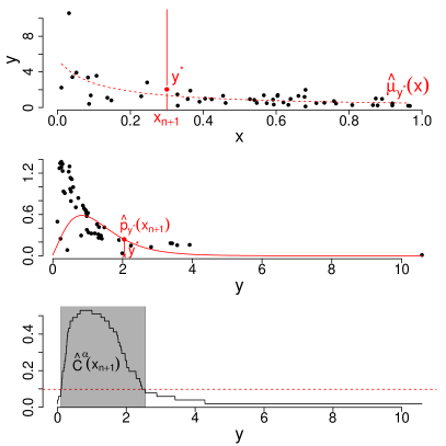
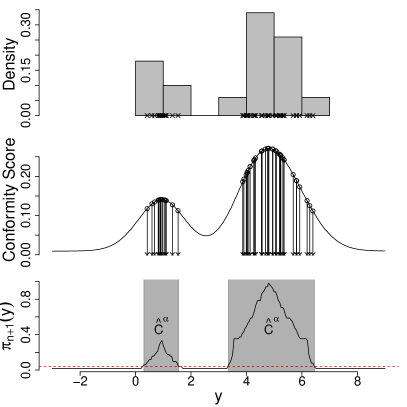
Figure 1 shows schematically how this conformal prediction region is constructed.
Refer to caption
Refer to caption
Figure 1: How conformal prediction regions are constructed. The left panel shows conformal prediction for a univariate outcome y𝑦y: the top row shows the data points and corresponding histogram; middle row shows conformity scores for a nonparametric kernel smoother; bottom panel shows πn+1,isubscript𝜋𝑛1𝑖\pi_{n+1,i} for each i𝑖i, and the conformal prediction set C^(α)superscript^𝐶𝛼\widehat{C}^{(\alpha)}. The right panel show conformal prediction for a univariate regression with predictor x𝑥x and outcome y𝑦y: the top row shows the (xi,yi)subscript𝑥𝑖subscript𝑦𝑖(x_{i},y_{i}) pairs, and a regression estimate μ^y(x)subscript^𝜇𝑦𝑥\hat{\mu}_{y}(x) computed using the additional point (xn+1,y)subscript𝑥𝑛1superscript𝑦(x_{n+1},y^{*}); middle panel shows the conformity scores obtained by using the estimated density as the conformity measure; bottom panel shows π(y)𝜋𝑦\pi(y) at xn+1subscript𝑥𝑛1x_{n+1}, the proportion of density scores lower than the density score at candidate y𝑦y, and the conformal prediction set C^(α)(xn+1)superscript^𝐶𝛼subscript𝑥𝑛1\widehat{C}^{(\alpha)}(x_{n+1}).

2.2 Notions of finite sample validity in regression

Several notions of finite sample validity exist in the context of regression. Suppose that we have an iid sample (Xi,Yi)subscript𝑋𝑖subscript𝑌𝑖(X_{i},Y_{i}), i=1𝑖1i=1, \ldots, n𝑛n where the predictor is Xm𝑋superscript𝑚X\in\mathbb{R}^{m} and Y𝑌Y\in\mathbb{R} is the outcome. We will suppose that d𝑑d of the X𝑋X’s are main effects, where dm𝑑𝑚d\leq m, and the other md𝑚𝑑m-d terms in X𝑋X are functions of the d𝑑d main effects. We will suppose that X𝑋X has support 𝒳=[0,1]d𝒳superscript01𝑑\mathcal{X}=[0,1]^{d}.

Definition 1 (marginal validity).

Let 0<α<10𝛼10<\alpha<1 be a desired error tolerance. Let (Xi,Yi)subscript𝑋𝑖subscript𝑌𝑖(X_{i},Y_{i}), i=1𝑖1i=1, \ldots, n𝑛n be an iid sample from a continuous distribution P𝑃P. The prediction region C^(α)superscript^𝐶𝛼\widehat{C}^{(\alpha)} has finite sample marginal validity if {Yn+1C^(α)(Xn+1)}1α,subscript𝑌𝑛1superscript^𝐶𝛼subscript𝑋𝑛11𝛼\mathbb{P}\left\{Y_{n+1}\in\widehat{C}^{(\alpha)}(X_{n+1})\right\}\geq 1-\alpha, where (Xn+1,Yn+1)Psimilar-tosubscript𝑋𝑛1subscript𝑌𝑛1𝑃(X_{n+1},Y_{n+1})\sim P.

Finite sample marginal validity is guaranteed for conformal prediction methods by construction. Finite sample marginal validity alone may not be desirable when variability of the outcome is not constant across the support of the predictor. A second notion of finite sample validity arises by considering coverage of the prediction region conditional on a particular value of the predictor.

Definition 2 (conditional validity).

Let 0<α<10𝛼10<\alpha<1 be a desired error tolerance. Let (Xi,Yi)subscript𝑋𝑖subscript𝑌𝑖(X_{i},Y_{i}), i=1𝑖1i=1, \ldots, n𝑛n be an iid sample from a continuous distribution P𝑃P. The prediction region C^(α)superscript^𝐶𝛼\widehat{C}^{(\alpha)} has finite sample conditional validity at x𝑥x when {Yn+1C^(α)(x)|Xn+1=x}1α,conditional-setsubscript𝑌𝑛1superscript^𝐶𝛼𝑥subscript𝑋𝑛1𝑥1𝛼\mathbb{P}\left\{Y_{n+1}\in\widehat{C}^{(\alpha)}(x)|X_{n+1}=x\right\}\geq 1-\alpha, where (Xn+1,Yn+1)Psimilar-tosubscript𝑋𝑛1subscript𝑌𝑛1𝑃(X_{n+1},Y_{n+1})\sim P.

However, conditional validity at every x𝑥x is unattainable if we insist that C^(α)superscript^𝐶𝛼\widehat{C}^{(\alpha)} is asymptotically of minimal length. Let p(y|x)𝑝conditional𝑦𝑥p(y|x) be the conditional density corresponding to regression of y𝑦y on x𝑥x. Define sx(α)subscriptsuperscript𝑠𝛼𝑥s^{(\alpha)}_{x} to be the value such that P(Yn+1{y:p(y|x)sx(α)}|X=x)=1α𝑃subscript𝑌𝑛1conditionalconditional-set𝑦𝑝conditional𝑦𝑥subscriptsuperscript𝑠𝛼𝑥𝑋𝑥1𝛼P(Y_{n+1}\in\{y:p(y|x)\geq s^{(\alpha)}_{x}\}|X=x)=1-\alpha and define C(x)={y:p(y|x)sx(α)}𝐶𝑥conditional-set𝑦𝑝conditional𝑦𝑥subscriptsuperscript𝑠𝛼𝑥C(x)=\left\{y:p(y|x)\geq s^{(\alpha)}_{x}\right\} to be the optimal conditional prediction region (i.e., the minimal length prediction region). Let ν𝜈\nu be Lebesgue measure and let \triangle denote the symmetric set difference operator. Then there does not exist a finite sample conditional valid prediction region C^(α)(x)superscript^𝐶𝛼𝑥\widehat{C}^{(\alpha)}(x) such that supx𝒳ν{C^(α)(x)C(x)}𝑃0subscriptsupremum𝑥𝒳𝜈superscript^𝐶𝛼𝑥𝐶𝑥𝑃0\sup_{x\in\mathcal{X}}\nu\left\{\widehat{C}^{(\alpha)}(x)\triangle C(x)\right\}\overset{P}{\to}0 holds, a result due to Lemma 1 of Lei and Wasserman (2014). A third notion of finite sample validity relaxes the stringent requirement of conditional validity at every possible x𝑥x.

Definition 3 (local validity).

Let 0<α<10𝛼10<\alpha<1 be a desired error tolerance. Let (Xi,Yi)subscript𝑋𝑖subscript𝑌𝑖(X_{i},Y_{i}), i=1𝑖1i=1, \ldots, n𝑛n be an iid sample from a continuous distribution P𝑃P. Let 𝒜={Ak:k1}𝒜conditional-setsubscript𝐴𝑘𝑘1\mathcal{A}=\{A_{k}:k\geq 1\} be a partition of 𝒳𝒳\mathcal{X}. We say that the prediction region C^(α)superscript^𝐶𝛼\widehat{C}^{(\alpha)} has finite sample local validity when {Yn+1C^(α)(Xn+1)|Xn+1Ak}1α,conditional-setsubscript𝑌𝑛1superscript^𝐶𝛼subscript𝑋𝑛1subscript𝑋𝑛1subscript𝐴𝑘1𝛼\mathbb{P}\left\{Y_{n+1}\in\widehat{C}^{(\alpha)}(X_{n+1})|X_{n+1}\in A_{k}\right\}\geq 1-\alpha, for all Ak𝒜subscript𝐴𝑘𝒜A_{k}\in\mathcal{A} where (Xn+1,Yn+1)Psimilar-tosubscript𝑋𝑛1subscript𝑌𝑛1𝑃(X_{n+1},Y_{n+1})\sim P.

Local validity offers a bridge between marginal validity – which is inappropriate in the presence of heterogeneity – and conditional validity – which is unattainable when we require that the prediction interval is asymptotically minimal (Lei and Wasserman, 2014). The nonparametric conformal prediction region in Section 4.1 satisfies finite sample local validity and is asymptotically conditional valid (Lei and Wasserman, 2014). In Section 3 we show that the parametric conformal prediction region also satisfies finite sample local validity and is asymptotically conditional valid at rate faster than its nonparametric counterpart.

3 Conformal prediction for parametric models

We now introduce parametric conformal prediction regions for a wide class of parametric families with continuous outcomes. We show that this class of parametric families includes continuous regular full exponential families, and hence GLMs by extension. Two parametric conformal prediction regions are provided. The first of these guarantees finite-sample local validity using a similar binning technique as Lei and Wasserman (2014). The second guarantees finite-sample marginal validity via transformation to a “common” distribution.

Suppose, for simplicity, that the support of the predictors is 𝒳=[0,1]d𝒳superscript01𝑑\mathcal{X}=[0,1]^{d}. Let (X,Y)Psimilar-to𝑋𝑌𝑃(X,Y)\sim P and let (Xi,Yi)Psimilar-tosubscript𝑋𝑖subscript𝑌𝑖𝑃(X_{i},Y_{i})\sim P, i=1𝑖1i=1, \ldots, n𝑛n be an iid sample where P𝑃P is a continuous distribution, Y𝑌Y\in\mathbb{R}, Xm𝑋superscript𝑚X\in\mathbb{R}^{m} with dm𝑑𝑚d\leq m main effects. We will denote the true conditional density of the regression model as pψ(|x)p_{\psi}(\cdot|x) and define ψr𝜓superscript𝑟\psi\in\mathbb{R}^{r}. For each x𝑥x, we define tx(α)subscriptsuperscript𝑡𝛼𝑥t^{(\alpha)}_{x} to be the point such that ({y:pψ(y|x)tx(α)}|X=x)=1αconditionalconditional-set𝑦subscript𝑝𝜓conditional𝑦𝑥subscriptsuperscript𝑡𝛼𝑥𝑋𝑥1𝛼\mathbb{P}\left(\{y:p_{\psi}(y|x)\geq t^{(\alpha)}_{x}\}|X=x\right)=1-\alpha for 0<α<10𝛼10<\alpha<1. The optimal or minimal length prediction region at x𝑥x is CP(α)(x)={y:pψ(y|x)tx(α)}subscriptsuperscript𝐶𝛼𝑃𝑥conditional-set𝑦subscript𝑝𝜓conditional𝑦𝑥subscriptsuperscript𝑡𝛼𝑥C^{(\alpha)}_{P}(x)=\{y:p_{\psi}(y|x)\geq t^{(\alpha)}_{x}\}. Define the moment generating function (MGF) MY,x,ψ(t)subscript𝑀𝑌𝑥𝜓𝑡M_{Y,x,\psi}(t) corresponding to the conditional density pψ(|x)p_{\psi}(\cdot|x). The parameter space for this parametric family is

𝒳={ψ:ψlogpψ(y|x)=O(y),MY,x,ψ(t)exists for alltin a neighborhood of 0,allx𝒳}.subscript𝒳conditional-set𝜓formulae-sequencesubscript𝜓subscript𝑝𝜓conditional𝑦𝑥𝑂𝑦subscript𝑀𝑌𝑥𝜓𝑡exists for all𝑡in a neighborhood of 0all𝑥𝒳\aleph_{\mathcal{X}}=\{\psi:\nabla_{\psi}\log p_{\psi}(y|x)=O(y),\;M_{Y,x,\psi}(t)\;\text{exists for all}\;t\;\text{in a neighborhood of}\;0,\;\text{all}\;x\in\mathcal{X}\;\}.

3.1 Local validity via binning

Let 𝒜={Ak:k1}𝒜conditional-setsubscript𝐴𝑘𝑘1\mathcal{A}=\{A_{k}:k\geq 1\} be a partition 𝒳𝒳\mathcal{X} and define the rates rn=O(log(n)/n)subscript𝑟𝑛𝑂𝑛𝑛r_{n}=O(\sqrt{\log(n)/n}) and zn=O{(log(n)/n)1/d}subscript𝑧𝑛𝑂superscript𝑛𝑛1𝑑z_{n}=O\{(\log(n)/n)^{1/d}\}. The number of elements in the partition 𝒜𝒜\mathcal{A} increases at rate 1/rn1subscript𝑟𝑛1/r_{n} when d2𝑑2d\leq 2 and 1/zn1subscript𝑧𝑛1/z_{n} when d>2𝑑2d>2. When we restrict the partition to be formed of equilateral cubes, we let the widths of these cubes decrease at rate rnsubscript𝑟𝑛r_{n} or znsubscript𝑧𝑛z_{n}. Let pψ(y|x)subscript𝑝𝜓conditional𝑦𝑥p_{\psi}(y|x) be the true conditional density function and let p^ψ(|)\hat{p}_{\psi}(\cdot|\cdot) be the estimated density fit using the original data and define p^ψ(x,y)(|)\hat{p}_{\psi}^{(x,y)}(\cdot|\cdot) as the estimated density fit to the augmented data {(X1,Y1),,(Xn,Yn),(x,y)}subscript𝑋1subscript𝑌1subscript𝑋𝑛subscript𝑌𝑛𝑥𝑦\{(X_{1},Y_{1}),\ldots,(X_{n},Y_{n}),(x,y)\}. We will use this estimated density as our conformity measure. The local conformal prediction region is then

C^n,k(α)(x)={y:1nk+1i=1n+1𝟙{XiAk}𝟙{p^ψ(x,y)(Yi|Xi)p^ψ(x,y)(y|x)}α~k},subscriptsuperscript^𝐶𝛼𝑛𝑘𝑥conditional-set𝑦1subscript𝑛𝑘1superscriptsubscript𝑖1𝑛11subscript𝑋𝑖subscript𝐴𝑘1superscriptsubscript^𝑝𝜓𝑥𝑦conditionalsubscript𝑌𝑖subscript𝑋𝑖superscriptsubscript^𝑝𝜓𝑥𝑦conditional𝑦𝑥subscript~𝛼𝑘\widehat{C}^{(\alpha)}_{n,k}(x)=\left\{y:\frac{1}{n_{k}+1}\sum_{i=1}^{n+1}\mathds{1}\left\{X_{i}\in A_{k}\right\}\mathds{1}\left\{\hat{p}_{\psi}^{(x,y)}(Y_{i}|X_{i})\leq\hat{p}_{\psi}^{(x,y)}(y|x)\right\}\geq\widetilde{\alpha}_{k}\right\}, (2)

where α~k=(nk+1)α/(nk+1)subscript~𝛼𝑘subscript𝑛𝑘1𝛼subscript𝑛𝑘1\widetilde{\alpha}_{k}=\lfloor(n_{k}+1)\alpha\rfloor/(n_{k}+1) for 0<α<10𝛼10<\alpha<1.

A schematic of how this conformal prediction region is constructed is displayed in the right-hand side of Figure 1. We now establish local validity for C^n,k(α)subscriptsuperscript^𝐶𝛼𝑛𝑘\widehat{C}^{(\alpha)}_{n,k}.

Lemma 2.

Let 𝒜𝒜\mathcal{A} be a partition of 𝒳𝒳\mathcal{X} and let C^n,k(α)(x)subscriptsuperscript^𝐶𝛼𝑛𝑘𝑥\widehat{C}^{(\alpha)}_{n,k}(x) be as defined in (2). Then C^n,k(α)(x)subscriptsuperscript^𝐶𝛼𝑛𝑘𝑥\widehat{C}^{(\alpha)}_{n,k}(x) is finite sample locally valid for xAk𝒜𝑥subscript𝐴𝑘𝒜x\in A_{k}\in\mathcal{A}.

Proof.

The proof follows from the proof of (Lei and Wasserman, 2014, Proposition 2). Fix k𝑘k and let {i1\{i_{1}, \ldots, ink}={i:1ini_{n_{k}}\}=\{i:1\leq i\leq n, XiAk}X_{i}\in A_{k}\}. Let (Xn+1(X_{n+1}, Yn+1)PY_{n+1})\sim P be another independent sample. Let ink+1=n+1subscript𝑖subscript𝑛𝑘1𝑛1i_{n_{k+1}}=n+1 and σij=p^ψ(x,y)(Yij|Xj)subscript𝜎subscript𝑖𝑗superscriptsubscript^𝑝𝜓𝑥𝑦conditionalsubscript𝑌subscript𝑖𝑗subscript𝑋𝑗\sigma_{i_{j}}=\hat{p}_{\psi}^{(x,y)}(Y_{i_{j}}|X_{j}) for all 1jnk+11𝑗subscript𝑛𝑘11\leq j\leq n_{k}+1. Then conditioning on Xn+1Aksubscript𝑋𝑛1subscript𝐴𝑘X_{n+1}\in A_{k} and (i1(i_{1}, \ldots, ink)i_{n_{k}}), the sequence (σi1(\sigma_{i_{1}}, \ldots, σinksubscript𝜎subscript𝑖subscript𝑛𝑘\sigma_{i_{n_{k}}}, σink+1)\sigma_{i_{n_{k}+1}}) is exchangeable. ∎

We now establish that the parametric conformal prediction region C^n,k(α)subscriptsuperscript^𝐶𝛼𝑛𝑘\widehat{C}^{(\alpha)}_{n,k} is asymptotically of minimum length over 𝒳𝒳\mathcal{X}.

Assumption 1 (Assumption 1 (a) of Lei and Wasserman (2014)). Let 𝒳𝒳\mathcal{X} be the support of X𝑋X and assume that 𝒳=[0,1]d𝒳superscript01𝑑\mathcal{X}=[0,1]^{d}. The marginal density of X𝑋X satisfies 0<b1pX(x)b2<0subscript𝑏1subscript𝑝𝑋𝑥subscript𝑏20<b_{1}\leq p_{X}(x)\leq b_{2}<\infty for all x𝒳𝑥𝒳x\in\mathcal{X}.

Assumption 2. The conditional density pψ(|x)p_{\psi}(\cdot|x) is Lipschitz in both x𝑥x and ψ𝜓\psi, there exists some L1,L2subscript𝐿1subscript𝐿2L_{1},L_{2}\in\mathbb{R} such that, pψ(|x1)pψ(|x2)L1x1x2,\|p_{\psi}(\cdot|x_{1})-p_{\psi}(\cdot|x_{2})\|_{\infty}\leq L_{1}\|x_{1}-x_{2}\|, and pψ1(|x)pψ2(|x)L2ψ1ψ2.\|p_{\psi_{1}}(\cdot|x)-p_{\psi_{2}}(\cdot|x)\|_{\infty}\leq L_{2}\|\psi_{1}-\psi_{2}\|.

Assumption 3 (smoothness condition of Lei and Wasserman (2014)). There exists positive constants ε,γ,c1𝜀𝛾subscript𝑐1\varepsilon,\gamma,c_{1}, and c2subscript𝑐2c_{2} such that, for all x𝒳𝑥𝒳x\in\mathcal{X}, and all ψ𝒳𝜓subscript𝒳\psi\in\aleph_{\mathcal{X}},

c1εγ[{y:|pψ(y|x)tx(α)|X=x}]c2εγ,c_{1}\varepsilon^{\gamma}\leq\mathbb{P}[\{y:|p_{\psi}(y|x)-t_{x}^{(\alpha)}|X=x\}]\leq c_{2}\varepsilon^{\gamma},

for all εε0𝜀subscript𝜀0\varepsilon\leq\varepsilon_{0}. Moreover, infxtx(α)t0>0subscriptinfimum𝑥superscriptsubscript𝑡𝑥𝛼subscript𝑡00\inf_{x}t_{x}^{(\alpha)}\geq t_{0}>0.

Theorem 1.

Let Y|X=xconditional𝑌𝑋𝑥Y|X=x be a random variable with conditional density pψ(|x)p_{\psi}(\cdot|x) and parameter space 𝒳subscript𝒳\aleph_{\mathcal{X}}. Assume that pψ(|x)p_{\psi}(\cdot|x) is twice differentiable in ψ𝜓\psi and satisfies Assumptions 2 and 3. Let (X1,Y1)subscript𝑋1subscript𝑌1(X_{1},Y_{1}), \ldots, (Xn,Yn)subscript𝑋𝑛subscript𝑌𝑛(X_{n},Y_{n}) be independent and identically distributed copies of (X,Y)𝑋𝑌(X,Y). Let ψr𝜓superscript𝑟\psi\in\mathbb{R}^{r}. Let ψ^^𝜓\hat{\psi} be the MLE of ψ𝜓\psi. Augment the sample data with a new point (x,y)𝑥𝑦(x,y), and let ψ^(x,y)superscript^𝜓𝑥𝑦\hat{\psi}^{(x,y)} be the MLE of ψ𝜓\psi with respect to the augmented data. Let p^ψ(x,y)(|x)\hat{p}^{(x,y)}_{\psi}(\cdot|x) be the conditional density with ψ^(x,y)superscript^𝜓𝑥𝑦\hat{\psi}^{(x,y)} plugged in for ψ𝜓\psi. Suppose that Assumption 1 holds. Let 0<α<10𝛼10<\alpha<1 and C^n,k(α)subscriptsuperscript^𝐶𝛼𝑛𝑘\widehat{C}^{(\alpha)}_{n,k} be the prediction band given by (2). Then, for a given λ>0𝜆0\lambda>0, there exists a numerical constant ζλsubscript𝜁𝜆\zeta_{\lambda} such that

[supx𝒳ν{C^n,k(α)(x)CP(α)(x)}ζλ(znrn)]=O(nλ),delimited-[]subscriptsupremum𝑥𝒳𝜈subscriptsuperscript^𝐶𝛼𝑛𝑘𝑥superscriptsubscript𝐶𝑃𝛼𝑥subscript𝜁𝜆subscript𝑧𝑛subscript𝑟𝑛𝑂superscript𝑛𝜆\mathbb{P}\left[\sup_{x\in\mathcal{X}}\nu\left\{\widehat{C}^{(\alpha)}_{n,k}(x)\triangle C_{P}^{(\alpha)}(x)\right\}\geq\zeta_{\lambda}(z_{n}\vee r_{n})\right]=O\left(n^{-\lambda}\right), (3)

where rn=O(log(n)/n)subscript𝑟𝑛𝑂𝑛𝑛r_{n}=O(\sqrt{\log(n)/n}).

Remarks:

  1. 1.

    The proof of Theorem 1 is given in the Appendix. The rates rnsubscript𝑟𝑛r_{n} and znsubscript𝑧𝑛z_{n} are appreciably faster than that of the nonparametric conformal prediction band which has a convergence rate of wn=O{log(n)/n}1/(d+3)subscript𝑤𝑛𝑂superscript𝑛𝑛1𝑑3w_{n}=O\{\log(n)/n\}^{1/(d+3)} when the underlying pψ(y|x)subscript𝑝𝜓conditional𝑦𝑥p_{\psi}(y|x) has parameter space 𝒳subscript𝒳\aleph_{\mathcal{X}}. The difference between the convergence speed of the parametric and nonparametric conformal prediction regions originates from the differences in the rates of MLEs and nonparametric techniques and the speed at which the bin widths shrink.

  2. 2.

    The following Lemma governs how fast the bins can shrink while still maintaining that nksubscript𝑛𝑘n_{k}\to\infty.

    Lemma 3 (Lemma 9 in Lei and Wasserman (2014)).

    Under Assumption 1, there exists constants C1subscript𝐶1C_{1} and C2subscript𝐶2C_{2} such that

    (k:b1nwnd/2nk3b2nwnd/2)1C1wndexp(C2nwnd),\mathbb{P}\left(\forall k:b_{1}nw_{n}^{d}/2\leq n_{k}\leq 3b_{2}nw_{n}^{d}/2\right)\geq 1-C_{1}w_{n}^{-d}\exp(-C_{2}nw_{n}^{d}),

    with b1subscript𝑏1b_{1} and b2subscript𝑏2b_{2} defined in Assumption 1.

  3. 3.

    The key term in Lemma 3 is the nwnd𝑛superscriptsubscript𝑤𝑛𝑑nw_{n}^{d} term appearing in the exponent. The proof of Theorem 1 reveals that the rate of convergence of the parametric conformal prediction region is limited by Lemma 3. This is not the case for the nonparametric conformal prediction region where the limiting factor is the rate of convergence of the kernel density estimator.

  4. 4.

    The proof of Theorem 1 requires a new concentration inequality for MLEs which is stated below as Theorem 4. The proof technique that we employ for Theorem 1 involves sandwiching C^n,k(α)(x)subscriptsuperscript^𝐶𝛼𝑛𝑘𝑥\widehat{C}^{(\alpha)}_{n,k}(x) by two estimated level sets, formalized as Lemma 10 in the Appendix. The convergence rate of these sandwiching level sets depends on rnsubscript𝑟𝑛r_{n}, znsubscript𝑧𝑛z_{n}, and the convergence rate of supx𝒳p^ψ(x,y)(|x)pψ(|x),\sup_{x\in\mathcal{X}}\|\hat{p}_{\psi}^{(x,y)}(\cdot|x)-p_{\psi}(\cdot|x)\|_{\infty}, see Lemma 9 in the Appendix. We verify that

    supx𝒳p^ψ(x,y)(|x)pψ(|x)=O(|ψ^ψ|),\sup_{x\in\mathcal{X}}\|\hat{p}_{\psi}^{(x,y)}(\cdot|x)-p_{\psi}(\cdot|x)\|_{\infty}=O\left(|\hat{\psi}-\psi|\right),

    where ψr𝜓superscript𝑟\psi\in\mathbb{R}^{r} are the parameters in density pψ(|x)p_{\psi}(\cdot|x) and ψ^^𝜓\hat{\psi} be the MLE of ψ𝜓\psi, hence the need for Theorem 4.

Let |||\cdot| denote the L1superscript𝐿1L^{1} norm of a vector or the absolute value of a scalar.

Theorem 2.

Let Y|X=xconditional𝑌𝑋𝑥Y|X=x be a random variable with conditional density pψ(|x)p_{\psi}(\cdot|x) and parameter space 𝒳subscript𝒳\aleph_{\mathcal{X}}. Assume that pψ(|x)p_{\psi}(\cdot|x) is twice differentiable in ψ𝜓\psi and satisfies Assumption 2. Let (X1,Y1)subscript𝑋1subscript𝑌1(X_{1},Y_{1}), \ldots, (Xn,Yn)subscript𝑋𝑛subscript𝑌𝑛(X_{n},Y_{n}) be independent and identically distributed copies of (X,Y)𝑋𝑌(X,Y). Let ψr𝜓superscript𝑟\psi\in\mathbb{R}^{r}. Let ψ^^𝜓\hat{\psi} be the MLE of ψ𝜓\psi. Then for any λ>0𝜆0\lambda>0, there exists a numerical constant Aλsubscript𝐴𝜆A_{\lambda}, such that

{n|ψ^ψ|Aλlog(n)}=O(nλ).𝑛^𝜓𝜓subscript𝐴𝜆𝑛𝑂superscript𝑛𝜆\mathbb{P}\left\{\sqrt{n}\left|\hat{\psi}-\psi\right|\geq A_{\lambda}\sqrt{\log(n)}\right\}=O\left(n^{-\lambda}\right). (4)

The concentration inequality given in Theorem 4 is a generalization of Theorem 3.3 in Miao (2010) to subexponential random variables with powers of log(n)/n𝑛𝑛\log(n)/n replacing r𝑟r, provided that the underlying density is parameterized with Xsubscript𝑋\aleph_{X}. Theorem 3.3 in Miao (2010) only holds for subgaussian random variables. Our extension is possible because of subexponential concentration theory and the score function is of the same order as the outcome variable. These results circumvent the necessity for the use of optimal transport theory (Bobkov and Götze, 1999; Ledoux, 1999, 2001; Djellout et al., 2004; Villani, 2008) to prove Theorem 3.3 in Miao (2010).

3.2 Transformation conformal

Transformation parametric conformal prediction was proposed by Chernozhukov et al. (2019) to construct a (1α)×100%1𝛼percent100(1-\alpha)\times 100\% prediction region using the lower and upper α/2𝛼2\alpha/2 quantiles of the assumed parametric distribution. We build on this framework to propose transformation based parametric conformal prediction regions that are asymptotically minimal length at rate rnsubscript𝑟𝑛r_{n}. Let m(x,ψ)𝑚𝑥𝜓m(x,\psi) be the number of modes of pψ(|x)p_{\psi}(\cdot|x) and suppose that supx𝒳,ψXm(x,ψ)=m<subscriptsupremumformulae-sequence𝑥𝒳𝜓subscript𝑋𝑚𝑥𝜓𝑚\sup_{x\in\mathcal{X},\,\psi\in\aleph_{X}}m(x,\psi)=m<\infty. With this specification we can construct CP(x)subscript𝐶𝑃𝑥C_{P}(x) as a finite union of intervals. Let F(|x)F(\cdot|x) be the conditional distribution function with density pψ(|x)p_{\psi}(\cdot|x) and let F^(|x)\widehat{F}(\cdot|x) be the estimate of F(|x)F(\cdot|x) with the MLE ψ^^𝜓\hat{\psi} plugged in. Let F^(x,y)(|)\widehat{F}^{(x,y)}(\cdot|\cdot) be the estimate of F(|)F(\cdot|\cdot) with the MLE corresponding to the augmented data ψ^(x,y)superscript^𝜓𝑥𝑦\hat{\psi}^{(x,y)} plugged in. Let (Xn+1,Yn+1)=(x,y)subscript𝑋𝑛1subscript𝑌𝑛1𝑥𝑦(X_{n+1},Y_{n+1})=(x,y) be a candidate data point.

The logic of transformation conformal prediction is as follows. We first augment the original data by adding the point (x,y)𝑥𝑦(x,y). We then estimate model parameters via maximum likelihood estimation with respect to this augmented dataset, and denote this estimator as ψ^(x,y)superscript^𝜓𝑥𝑦\hat{\psi}^{(x,y)}. The estimator ψ^(x,y)superscript^𝜓𝑥𝑦\hat{\psi}^{(x,y)} is then used to estimate the distribution function F(|)F(\cdot|\cdot) by F^(x,y)(|)\widehat{F}^{(x,y)}(\cdot|\cdot) via plugin. We then transform outcomes by computing U^i(x,y)=F^(x,y)(Yi|Xi)subscriptsuperscript^𝑈𝑥𝑦𝑖superscript^𝐹𝑥𝑦conditionalsubscript𝑌𝑖subscript𝑋𝑖\widehat{U}^{(x,y)}_{i}=\widehat{F}^{(x,y)}(Y_{i}|X_{i}) for i=1,,n+1𝑖1𝑛1i=1,\ldots,n+1. Define π~(y)=(n+1)1i=1n+1𝟙{σ(U^i(x,y))σ(U^n+1(x,y))},~𝜋𝑦superscript𝑛11superscriptsubscript𝑖1𝑛11𝜎subscriptsuperscript^𝑈𝑥𝑦𝑖𝜎subscriptsuperscript^𝑈𝑥𝑦𝑛1\tilde{\pi}(y)=(n+1)^{-1}\sum_{i=1}^{n+1}\mathds{1}\left\{\sigma\left(\widehat{U}^{(x,y)}_{i}\right)\leq\sigma\left(\widehat{U}^{(x,y)}_{n+1}\right)\right\}, and the conformal prediction region

C~(α)(x)={y:π~(y)α},superscript~𝐶𝛼𝑥conditional-set𝑦~𝜋𝑦superscript𝛼\widetilde{C}^{(\alpha)}(x)=\left\{y:\tilde{\pi}(y)\geq\alpha^{\prime}\right\}, (5)

where 0<αα<10superscript𝛼𝛼10<\alpha^{\prime}\leq\alpha<1.

Lemma 4.

Let C~(α)(x)superscript~𝐶𝛼𝑥\widetilde{C}^{(\alpha)}(x) be as defined in (5). Then C~(α)(x)superscript~𝐶𝛼𝑥\widetilde{C}^{(\alpha)}(x) is finite sample marginally valid.

Proof.

The proof follows from the proof of Lemma 2. Let (Xn+1(X_{n+1}, Yn+1)PY_{n+1})\sim P be another independent sample. The random variables U^i(x,y)subscriptsuperscript^𝑈𝑥𝑦𝑖\widehat{U}^{(x,y)}_{i}, 1in+11𝑖𝑛11\leq i\leq n+1, are exchangeable. Then, conditioning on Xn+1=xsubscript𝑋𝑛1𝑥X_{n+1}=x, the sequence (σ(U^1(x,y)),,σ(U^n+1(x,y)))𝜎subscriptsuperscript^𝑈𝑥𝑦1𝜎subscriptsuperscript^𝑈𝑥𝑦𝑛1\left(\sigma(\widehat{U}^{(x,y)}_{1}),\ldots,\sigma(\widehat{U}^{(x,y)}_{n+1})\right) is exchangeable. Marginal validity follows by construction. ∎

A particular choice of the conformity measure σ()𝜎\sigma(\cdot) and αsuperscript𝛼\alpha^{\prime} yields an asymptotically minimal length conformal prediction region at rate rnsubscript𝑟𝑛r_{n}. First, let U^n+1(x,y)=F^(x,y)(y|x)subscriptsuperscript^𝑈𝑥𝑦𝑛1superscript^𝐹𝑥𝑦conditional𝑦𝑥\widehat{U}^{(x,y)}_{n+1}=\widehat{F}^{(x,y)}(y|x) be the transformed augmented outcome. We can find a minimal length 1α1𝛼1-\alpha high density region based on the estimated density p^ψ(x,y)(|x)\hat{p}_{\psi}^{(x,y)}(\cdot|x) through solution of the optimization problem

A^(x)=argminA(x)ν(A(x)),subject toA(x)p^ψ(x,y)(y|x)𝑑y=1α,formulae-sequence^𝐴𝑥subscriptargmin𝐴𝑥𝜈𝐴𝑥subject tosubscript𝐴𝑥superscriptsubscript^𝑝𝜓𝑥𝑦conditionalsuperscript𝑦𝑥differential-dsuperscript𝑦1𝛼\hat{A}(x)=\text{argmin}_{A(x)}\nu(A(x)),\qquad\text{subject to}\qquad\int_{A(x)}\hat{p}_{\psi}^{(x,y)}(y^{\prime}|x)dy^{\prime}=1-\alpha, (6)

where the solution A^(x)=k=1m(x)(a^k(x),b^k(x))^𝐴𝑥superscriptsubscript𝑘1superscript𝑚𝑥subscript^𝑎𝑘𝑥subscript^𝑏𝑘𝑥\hat{A}(x)=\cup_{k=1}^{m^{\prime}(x)}(\hat{a}_{k}(x),\hat{b}_{k}(x)) is a union of m(x)superscript𝑚𝑥m^{\prime}(x) disjoint intervals. Because pψ(|x)p_{\psi}(\cdot|x) has m<𝑚m<\infty modes for every x𝒳𝑥𝒳x\in\mathcal{X}, the number of intervals in the union is m(x)msuperscript𝑚𝑥𝑚m^{\prime}(x)\leq m. Let

U^lwr,k(x,y)=F^(x,y)(a^k(x)|x)andU^upr,k(x,y)=F^(x,y)(b^k(x)|x)formulae-sequencesubscriptsuperscript^𝑈𝑥𝑦lwr𝑘superscript^𝐹𝑥𝑦conditionalsubscript^𝑎𝑘𝑥𝑥andsubscriptsuperscript^𝑈𝑥𝑦upr𝑘superscript^𝐹𝑥𝑦conditionalsubscript^𝑏𝑘𝑥𝑥\widehat{U}^{(x,y)}_{\text{lwr},k}=\widehat{F}^{(x,y)}(\hat{a}_{k}(x)|x)\quad\text{and}\quad\widehat{U}^{(x,y)}_{\text{upr},k}=\widehat{F}^{(x,y)}(\hat{b}_{k}(x)|x)

be the transformed values corresponding to the lower and upper limits of the prediction set for each x𝒳𝑥𝒳x\in\mathcal{X}.

Then, for each k𝑘k, find intervals in the transformed observed values that contain (ak(x),bk(x))subscript𝑎𝑘𝑥subscript𝑏𝑘𝑥(a_{k}(x),b_{k}(x)),

U~lwr,k(x,y)={U^[(n+1)U^lwr,k(x,y)](x,y)if (n+1)U^lwr,k(x,y)10otherwisesubscriptsuperscript~𝑈𝑥𝑦lwr𝑘casessubscriptsuperscript^𝑈𝑥𝑦delimited-[]𝑛1subscriptsuperscript^𝑈𝑥𝑦lwr𝑘if 𝑛1subscriptsuperscript^𝑈𝑥𝑦lwr𝑘10otherwise\widetilde{U}^{(x,y)}_{\text{lwr},k}=\begin{cases}\widehat{U}^{(x,y)}_{\left[\lfloor(n+1)\widehat{U}^{(x,y)}_{\text{lwr},k}\rfloor\right]}&\text{if }\lfloor(n+1)\widehat{U}^{(x,y)}_{\text{lwr},k}\rfloor\geq 1\\ 0&\text{otherwise}\end{cases}

and U~upr,k(x,y)=U^[(n+1)U^upr,k(x,y)](x,y)subscriptsuperscript~𝑈𝑥𝑦upr𝑘subscriptsuperscript^𝑈𝑥𝑦delimited-[]𝑛1subscriptsuperscript^𝑈𝑥𝑦upr𝑘\widetilde{U}^{(x,y)}_{\text{upr},k}=\widehat{U}^{(x,y)}_{\left[\lceil(n+1)\widehat{U}^{(x,y)}_{\text{upr},k}\rceil\right]} where U^[j](x,y)subscriptsuperscript^𝑈𝑥𝑦delimited-[]𝑗\widehat{U}^{(x,y)}_{[j]} is the j𝑗jth order statistic of the transformed values. Define the set consisting of the union of these intervals

B^(x,y)=k=1m(x)(U~lwr,k(x,y),U~upr,k(x,y)),superscript^𝐵𝑥𝑦superscriptsubscript𝑘1superscript𝑚𝑥subscriptsuperscript~𝑈𝑥𝑦lwr𝑘subscriptsuperscript~𝑈𝑥𝑦upr𝑘\widehat{B}^{(x,y)}=\cup_{k=1}^{m^{\prime}(x)}\left(\widetilde{U}^{(x,y)}_{\text{lwr},k},\widetilde{U}^{(x,y)}_{\text{upr},k}\right),

and define the conformity measure as the indicator that the value u𝑢u is in the estimated high density region, σ(u)=𝟙{uB^(x,y)}𝜎𝑢1𝑢superscript^𝐵𝑥𝑦\sigma(u)=\mathds{1}\{u\in\widehat{B}^{(x,y)}\}. Let the threshold be

α=1k=1m(x)((n+1)U~upr,k(x,y)n+1(n+1)U~lwr,k(x,y)n+1)α.superscript𝛼1superscriptsubscript𝑘1superscript𝑚𝑥𝑛1subscriptsuperscript~𝑈𝑥𝑦upr𝑘𝑛1𝑛1subscriptsuperscript~𝑈𝑥𝑦lwr𝑘𝑛1𝛼\alpha^{\prime}=1-\sum_{k=1}^{m^{\prime}(x)}\left(\frac{\lceil(n+1)\widetilde{U}^{(x,y)}_{\text{upr},k}\rceil}{n+1}-\frac{\lfloor(n+1)\widetilde{U}^{(x,y)}_{\text{lwr},k}\rfloor}{n+1}\right)\leq\alpha.

With these specifications, the conformal prediction region (5) becomes

C^trans(α)(x)={y:U^n+1(x,y)k=1m(x)(U~lwr,k(x,y),U~upr,k(x,y))},subscriptsuperscript^𝐶𝛼trans𝑥conditional-set𝑦subscriptsuperscript^𝑈𝑥𝑦𝑛1superscriptsubscript𝑘1superscript𝑚𝑥subscriptsuperscript~𝑈𝑥𝑦lwr𝑘subscriptsuperscript~𝑈𝑥𝑦upr𝑘\widehat{C}^{(\alpha)}_{\text{trans}}(x)=\left\{y:\widehat{U}^{(x,y)}_{n+1}\in\cup_{k=1}^{m^{\prime}(x)}\left(\widetilde{U}^{(x,y)}_{\text{lwr},k},\widetilde{U}^{(x,y)}_{\text{upr},k}\right)\right\}, (7)

where yC^trans(α)(x)𝑦subscriptsuperscript^𝐶𝛼trans𝑥y\in\widehat{C}^{(\alpha)}_{\text{trans}}(x) implies that σ(U^n+1(x,y))=1𝜎subscriptsuperscript^𝑈𝑥𝑦𝑛11\sigma(\widehat{U}^{(x,y)}_{n+1})=1.

While this procedure may appear complicated, it is motivated by a simple observation. When the parametric model is correctly specified, the U^i(x,y)subscriptsuperscript^𝑈𝑥𝑦𝑖\widehat{U}^{(x,y)}_{i} random variables have an approximate Uniform[0,1]01[0,1] distribution in finite samples and are asymptotically Uniform[0,1]01[0,1]. By conducting the conformal prediction procedure in the transformed space, we can leverage distributional information from the estimated density p^ψ(x,y)(|x)\hat{p}_{\psi}^{(x,y)}(\cdot|x) to mimic a highest density region while ensuring nominal marginal coverage. Even when the model is misspecified, this procedure is designed to guarantee nominal marginal coverage.

We now establish that the transformation parametric conformal prediction region C^trans(α)subscriptsuperscript^𝐶𝛼trans\widehat{C}^{(\alpha)}_{\text{trans}} is asymptotically of minimum length over 𝒳𝒳\mathcal{X} at rate rnsubscript𝑟𝑛r_{n}.

Assumption 4. Let Y|X=xconditional𝑌𝑋𝑥Y|X=x be a random variable with conditional density pψ(|x)p_{\psi}(\cdot|x) and parameter space 𝒳subscript𝒳\aleph_{\mathcal{X}}. Let F(y|x)𝐹conditional𝑦𝑥F(y|x) be the conditional distribution function corresponding to pψ(|x)p_{\psi}(\cdot|x). Further assume that |ψF(v|x)||\nabla_{\psi}F(v|x)| is bounded for all v𝑣v and all ψX𝜓subscript𝑋\psi\in\aleph_{X}.

Theorem 3.

Let Y|X=xconditional𝑌𝑋𝑥Y|X=x be a random variable with conditional density pψ(|x)p_{\psi}(\cdot|x) and parameter space 𝒳subscript𝒳\aleph_{\mathcal{X}}. Assume that pψ(|x)p_{\psi}(\cdot|x) has m𝑚m modes, is twice differentiable in ψ𝜓\psi, and satisfies Assumption 2. Assume that the corresponding distribution function satisfies Assumption 4. Let (X1,Y1)subscript𝑋1subscript𝑌1(X_{1},Y_{1}), \ldots, (Xn,Yn)subscript𝑋𝑛subscript𝑌𝑛(X_{n},Y_{n}) be independent and identically distributed copies of (X,Y)𝑋𝑌(X,Y). Let ψr𝜓superscript𝑟\psi\in\mathbb{R}^{r} and let ψ^^𝜓\hat{\psi} be the MLE of ψ𝜓\psi. Augment the sample data with a new point (x,y)𝑥𝑦(x,y), and let ψ^(x,y)superscript^𝜓𝑥𝑦\hat{\psi}^{(x,y)} be the MLE of ψ𝜓\psi with respect to the augmented data. Let p^ψ(x,y)(|x)\hat{p}^{(x,y)}_{\psi}(\cdot|x) be the conditional density with ψ^(x,y)superscript^𝜓𝑥𝑦\hat{\psi}^{(x,y)} plugged in for ψ𝜓\psi. Suppose that Assumption 1 holds. Let 0<α<10𝛼10<\alpha<1 and C^trans(α)subscriptsuperscript^𝐶𝛼trans\widehat{C}^{(\alpha)}_{\text{trans}} be the prediction band given by (7). Then, for a given λ>0𝜆0\lambda>0, there exists a numerical constant χλsubscript𝜒𝜆\chi_{\lambda} such that

[supx𝒳ν{C^trans(α)(x)CP(α)(x)}χλrn]=O(nλ).delimited-[]subscriptsupremum𝑥𝒳𝜈subscriptsuperscript^𝐶𝛼trans𝑥superscriptsubscript𝐶𝑃𝛼𝑥subscript𝜒𝜆subscript𝑟𝑛𝑂superscript𝑛𝜆\mathbb{P}\left[\sup_{x\in\mathcal{X}}\nu\left\{\widehat{C}^{(\alpha)}_{\text{trans}}(x)\triangle C_{P}^{(\alpha)}(x)\right\}\geq\chi_{\lambda}r_{n}\right]=O\left(n^{-\lambda}\right). (8)

Remarks:

  1. 1.

    In the simple case when pψ(y|x)subscript𝑝𝜓conditional𝑦𝑥p_{\psi}(y|x) is unimodal, the optimization problem (6) is replaced with,

    (a^(x),b^(x))=argmin(a,b)(ba),subject toabp^ψ(x,y)(u|x)𝑑u=1α,andba>0.formulae-sequence^𝑎𝑥^𝑏𝑥subscriptargmin𝑎𝑏𝑏𝑎subject toformulae-sequencesuperscriptsubscript𝑎𝑏superscriptsubscript^𝑝𝜓𝑥𝑦conditional𝑢𝑥differential-d𝑢1𝛼and𝑏𝑎0(\hat{a}(x),\hat{b}(x))=\text{argmin}_{(a,b)}\left(b-a\right),\qquad\text{subject to}\qquad\int_{a}^{b}\hat{p}_{\psi}^{(x,y)}(u|x)du=1-\alpha,\;\text{and}\;b-a>0. (9)

    In this case, we then construct U^lwr(x,y)=F^(x,y)(a^(x)|x)subscriptsuperscript^𝑈𝑥𝑦lwrsuperscript^𝐹𝑥𝑦conditional^𝑎𝑥𝑥\widehat{U}^{(x,y)}_{\text{lwr}}=\widehat{F}^{(x,y)}(\hat{a}(x)|x) and U^upr(x,y)=F^(x,y)(b^(x)|x)subscriptsuperscript^𝑈𝑥𝑦uprsuperscript^𝐹𝑥𝑦conditional^𝑏𝑥𝑥\widehat{U}^{(x,y)}_{\text{upr}}=\widehat{F}^{(x,y)}(\hat{b}(x)|x), and set B~(x,y)=(U^lwr(x,y),U^upr(x,y)).superscript~𝐵𝑥𝑦subscriptsuperscript^𝑈𝑥𝑦lwrsubscriptsuperscript^𝑈𝑥𝑦upr\widetilde{B}^{(x,y)}=(\widehat{U}^{(x,y)}_{\text{lwr}},\widehat{U}^{(x,y)}_{\text{upr}}). From these quantities, we construct the conformity measure σ(u)=𝟙(B~(x,y))(u),𝜎𝑢subscript1superscript~𝐵𝑥𝑦𝑢\sigma(u)=\mathds{1}_{(\widetilde{B}^{(x,y)})}(u), specify that

    α=1((n+1)U^upr(x,y)n+1(n+1)U^lwr(x,y)n+1)α,superscript𝛼1𝑛1subscriptsuperscript^𝑈𝑥𝑦upr𝑛1𝑛1subscriptsuperscript^𝑈𝑥𝑦lwr𝑛1𝛼\alpha^{\prime}=1-\left(\frac{\lceil(n+1)\widehat{U}^{(x,y)}_{\text{upr}}\rceil}{n+1}-\frac{\lfloor(n+1)\widehat{U}^{(x,y)}_{\text{lwr}}\rfloor}{n+1}\right)\leq\alpha,

    and build C~(α)(x)superscript~𝐶𝛼𝑥\widetilde{C}^{(\alpha)}(x) with respect to these specifications as

    C~(α)(x)={y:U^[(n+1)U^lwr(x,y)](x,y)U^n+1(x,y)U^[(n+1)U^upr(x,y)](x,y)},superscript~𝐶𝛼𝑥conditional-set𝑦subscriptsuperscript^𝑈𝑥𝑦delimited-[]𝑛1subscriptsuperscript^𝑈𝑥𝑦lwrsubscriptsuperscript^𝑈𝑥𝑦𝑛1subscriptsuperscript^𝑈𝑥𝑦delimited-[]𝑛1subscriptsuperscript^𝑈𝑥𝑦upr\widetilde{C}^{(\alpha)}(x)=\left\{y:\widehat{U}^{(x,y)}_{\left[\lfloor(n+1)\widehat{U}^{(x,y)}_{\text{lwr}}\rfloor\right]}\leq\widehat{U}^{(x,y)}_{n+1}\leq\widehat{U}^{(x,y)}_{\left[\lceil(n+1)\widehat{U}^{(x,y)}_{\text{upr}}\rceil\right]}\right\}, (10)

    where yC~(α)(x)𝑦superscript~𝐶𝛼𝑥y\in\widetilde{C}^{(\alpha)}(x) implies that σ(U^n+1(x,y))=1𝜎subscriptsuperscript^𝑈𝑥𝑦𝑛11\sigma(\widehat{U}^{(x,y)}_{n+1})=1.

  2. 2.

    The proof of Theorem 8 is given in the Appendix. Our proof technique is for the m=1𝑚1m=1 case. The proof of Theorem 8 requires the concentration inequality for MLEs stated in Theorem 4. Under our proof technique the convergence rate rn=log(n)/nsubscript𝑟𝑛𝑛𝑛r_{n}=\sqrt{\log(n)/n} of C^trans(α)subscriptsuperscript^𝐶𝛼trans\widehat{C}^{(\alpha)}_{\text{trans}} is sharp.

  3. 3.

    The rates rnsubscript𝑟𝑛r_{n} is appreciably faster than that of the nonparametric conformal prediction band and the binned parametric conformal prediction region C^n,k(α)subscriptsuperscript^𝐶𝛼𝑛𝑘\widehat{C}^{(\alpha)}_{n,k} in (2) when the underlying density pψ(y|x)subscript𝑝𝜓conditional𝑦𝑥p_{\psi}(y|x) has parameter space 𝒳subscript𝒳\aleph_{\mathcal{X}}. The region C^n,k(α)subscriptsuperscript^𝐶𝛼𝑛𝑘\widehat{C}^{(\alpha)}_{n,k} converges more slowly slower than C^trans(α)subscriptsuperscript^𝐶𝛼trans\widehat{C}^{(\alpha)}_{\text{trans}} because the former prediction region is hampered by nksubscript𝑛𝑘n_{k}, the number of observations per bin, as the bin widths shrink at rate wnsubscript𝑤𝑛w_{n}. However, our simulation studies show that C^n,k(α)subscriptsuperscript^𝐶𝛼𝑛𝑘\widehat{C}^{(\alpha)}_{n,k} performs better than C^trans(α)subscriptsuperscript^𝐶𝛼trans\widehat{C}^{(\alpha)}_{\text{trans}} when modest departures from the assumed model are present, due to its finite sample local validity guarantees.

  4. 4.

    The transformation parametric conformal prediction region in Chernozhukov et al. (2019) has generality beyond the context of the maximum likelihood estimation based methodology that we propose. However, explicit convergence rates for their conformal prediction rates are not given and we speculate that they would be slower for the entire class of models for which their methodology is appropriate. In addition, our methodology leverages the underlying true distribution to construct the minimal length (1α)×100%1𝛼percent100(1-\alpha)\times 100\% prediction region under the assumed model when on the scale of the approximately uniform random variables. This is instead of choosing the end points corresponding to the lower and upper α/2𝛼2\alpha/2 quantiles of the transformed approximate uniform variables. Our focus on minimal length prediction regions and relatively fast convergence rates addresses the efficiency and utility concerns of conformal prediction in the context of regression which were raised in Cortés-Ciriano and Bender (2019).

3.3 Example: exponential family distributions and generalized linear models

In this Section we show that a broad class of continuous GLMs can be parameterized by 𝒳subscript𝒳\aleph_{\mathcal{X}} so that the conformal prediction methodology is applicable. The exponential families that we consider have densities pθ:p:subscript𝑝𝜃superscript𝑝p_{\theta}:\mathbb{R}^{p}\to\mathbb{R} defined by

pθ(y)=ey,θc(θ).subscript𝑝𝜃𝑦superscript𝑒𝑦𝜃𝑐𝜃p_{\theta}(y)=e^{\langle y,\theta\rangle-c(\theta)}. (11)

We refer to y𝑦y and θ𝜃\theta as the canonical statistic and canonical parameter respectively. Densities of the form pθsubscript𝑝𝜃p_{\theta} are integrated with respect to a generating measure μ𝜇\mu, where c(θ)𝑐𝜃c(\theta) is the cumulant function defined as c(θ)=logexp(y,θ)μ(dy)𝑐𝜃𝑦𝜃𝜇𝑑𝑦c(\theta)=\log\int\exp(\langle y,\theta\rangle)\,\mu(dy). The effective domain of c𝑐c is domc={θ:c(θ)<+}.dom𝑐conditional-set𝜃𝑐𝜃\operatorname{dom}c=\left\{\theta\in\mathbb{R}:c(\theta)<+\infty\right\}. The exponential family is full if Θ=domcΘdom𝑐\Theta=\operatorname{dom}c and is regular if ΘΘ\Theta is an open set.

We will only consider scalar outcome variables. However, we can extend our setup to multidimensional canonical statistics, the normal distribution being an example with canonical statistic z(z,z2)maps-to𝑧superscript𝑧superscript𝑧2z\mapsto(z,z^{2})^{\prime}. Thus we will assume that the canonical statistic vector lies on a one-dimensional manifold in the event that the canonical statistic is multidimensional.

When the density (11) corresponds to a generalized linear regression model we will re-parameterize θ=f(xβ,ϕ)𝜃𝑓superscript𝑥𝛽italic-ϕ\theta=f(x^{\prime}\beta,\phi), where f:pp:𝑓superscript𝑝superscript𝑝f:\mathbb{R}^{p}\to\mathbb{R}^{p} is continuous in both arguments, the vectors xm𝑥superscript𝑚x\in\mathbb{R}^{m} and βm𝛽superscript𝑚\beta\in\mathbb{R}^{m} are a predictors and regression coefficients respectively, and ϕp1italic-ϕsuperscript𝑝1\phi\in\mathbb{R}^{p-1} is a vector of nuisance parameters. Let ψ=(β,ϕ)𝜓𝛽italic-ϕ\psi=(\beta,\phi) and set r=m+p1𝑟𝑚𝑝1r=m+p-1. We specify that the base set (main effects) of predictors have support 𝒳d𝒳superscript𝑑\mathcal{X}\in\mathbb{R}^{d}, dm𝑑𝑚d\leq m. Here we assume, without loss of generality, that 𝔼(Y1|x)=g1(xβ)𝔼conditionalsubscript𝑌1𝑥superscript𝑔1superscript𝑥𝛽\mathbb{E}(Y_{1}|x)=g^{-1}(x^{\prime}\beta) where g::𝑔g:\mathbb{R}\to\mathbb{R} is a link function and Y1subscript𝑌1Y_{1} is the first component of the canonical statistic vector. As an example of this reparameterization, consider the simple linear regression model with homoskedastic normal errors with variance given by σ2superscript𝜎2\sigma^{2}. In this example d=m=1𝑑𝑚1d=m=1, r=2𝑟2r=2, and ϕ=σ2italic-ϕsuperscript𝜎2\phi=\sigma^{2}. The link function g𝑔g is taken to be the identity function and μx=𝔼(Y|x)=xβsubscript𝜇𝑥𝔼conditional𝑌𝑥superscript𝑥𝛽\mu_{x}=\mathbb{E}(Y|x)=x^{\prime}\beta.

The reparameterized density corresponding to the generalized linear regression model is then

pψ(y|x)=exp[y,f(xβ,ϕ)c{f(xβ,ϕ)}]subscript𝑝𝜓conditional𝑦𝑥𝑦𝑓superscript𝑥𝛽italic-ϕ𝑐𝑓superscript𝑥𝛽italic-ϕp_{\psi}(y|x)=\exp\left[\langle y,f(x^{\prime}\beta,\phi)\rangle-c\left\{f(x^{\prime}\beta,\phi)\right\}\right] (12)

with respect to generating measure μ𝜇\mu. We will further assume that 𝒳𝒳\mathcal{X} is bounded and that the exponential family is full with parameter space given by Θ𝒳={βm,ϕp1:c{f(xβ,ϕ)}<,for allx𝒳}.subscriptΘ𝒳conditional-setformulae-sequence𝛽superscript𝑚italic-ϕsuperscript𝑝1formulae-sequence𝑐𝑓superscript𝑥𝛽italic-ϕfor all𝑥𝒳\Theta_{\mathcal{X}}=\{\beta\in\mathbb{R}^{m},\;\phi\in\mathbb{R}^{p-1}:c\left\{f(x^{\prime}\beta,\phi)\right\}<\infty,\;\text{for all}\;x\in\mathcal{X}\}. Consider the multiple linear regression model with homoskedastic normal errors with variance given by σ2superscript𝜎2\sigma^{2}. Here we have f(xβ,ϕ)=(xβ,σ2)𝑓superscript𝑥𝛽italic-ϕsuperscriptsuperscript𝑥𝛽superscript𝜎2f(x^{\prime}\beta,\phi)=(x^{\prime}\beta,\sigma^{2})^{\prime} and Θ𝒳={(β,σ2):βm,σ>0,x𝒳}.subscriptΘ𝒳conditional-setsuperscriptsuperscript𝛽superscript𝜎2formulae-sequence𝛽superscript𝑚formulae-sequence𝜎0𝑥𝒳\Theta_{\mathcal{X}}=\{(\beta^{\prime},\sigma^{2})^{\prime}:\beta\in\mathbb{R}^{m},\;\sigma>0,x\in\mathcal{X}\}. We will assume that the link function of the generalized linear regression model is known, the model is correctly specified, and that β^^𝛽\hat{\beta} is a n𝑛\sqrt{n}-consistent estimator of the regression coefficients β𝛽\beta. All of the continuous exponential families implemented in the glm function in R have densities that can be parameterized as (12). Moreover, we have that Θ𝒳𝒳subscriptΘ𝒳subscript𝒳\Theta_{\mathcal{X}}\subseteq\aleph_{\mathcal{X}} since,

ψlogpψ(y|x)=ψ(y,f(xβ,ϕ)c{f(xβ,ϕ)})𝜓subscript𝑝𝜓conditional𝑦𝑥𝜓𝑦𝑓superscript𝑥𝛽italic-ϕ𝑐𝑓superscript𝑥𝛽italic-ϕ\displaystyle\frac{\partial}{\partial\psi}\log p_{\psi}(y|x)=\frac{\partial}{\partial\psi}\left(\langle y,f(x^{\prime}\beta,\phi)\rangle-c\left\{f(x^{\prime}\beta,\phi)\right\}\right)
=(f(xβ,ϕ)ψ)(yf(xβ,ϕ)c{f(xβ,ϕ)})=O(y),absent𝑓superscript𝑥𝛽italic-ϕ𝜓𝑦𝑓superscript𝑥𝛽italic-ϕ𝑐𝑓superscript𝑥𝛽italic-ϕ𝑂𝑦\displaystyle\qquad=\left(\frac{\partial f(x^{\prime}\beta,\phi)}{\partial\psi}\right)\left(y-\frac{\partial}{\partial f(x^{\prime}\beta,\phi)}c\left\{f(x^{\prime}\beta,\phi)\right\}\right)=O(y),

and MY,x,ψ(t)subscript𝑀𝑌𝑥𝜓𝑡M_{Y,x,\psi}(t) exists for all t𝑡t in a neighborhood of 0, for all x𝒳𝑥𝒳x\in\mathcal{X} , and ψΘ𝒳𝜓subscriptΘ𝒳\psi\in\Theta_{\mathcal{X}}. Therefore our conformal prediction regions are appropriate for the GLMs parameterized in this Section. We show that our GLM parameterization satisfies Assumptions 2 and 3 in the Supplementary Materials.

We describe some related work on conformal prediction techniques for regression settings in the next sections. Finite-sample performance of our parametric conformal prediction region and these related methods is assessed in Section 5.

4 Existing conformal prediction techniques in regression

4.1 The nonparametric kernel estimator

Lei and Wasserman (2014) proposed a nonparametric conformal prediction region for continuous outcomes that satisfies finite sample local validity. Partitioning of the predictor space is performed so that the nonparametric conformal prediction region within each partition achieves finite sample marginal validity. When we restrict the partition to be formed of equilateral cubes, we let the widths of these cubes decrease at rate wnsubscript𝑤𝑛w_{n}. Let nk=i=1n1(XiAk)subscript𝑛𝑘superscriptsubscript𝑖1𝑛1subscript𝑋𝑖subscript𝐴𝑘n_{k}=\sum_{i=1}^{n}1(X_{i}\in A_{k}). Let K()𝐾K(\cdot) be a non-negative kernel function. The estimated local marginal density of Y𝑌Y is p~(v|Ak)=(nkhn)1i=1n𝟙{XiAk}K((Yiv)/hn)~𝑝conditional𝑣subscript𝐴𝑘superscriptsubscript𝑛𝑘subscript𝑛1superscriptsubscript𝑖1𝑛1subscript𝑋𝑖subscript𝐴𝑘𝐾subscript𝑌𝑖𝑣subscript𝑛\tilde{p}(v|A_{k})=(n_{k}h_{n})^{-1}\sum_{i=1}^{n}\mathds{1}\left\{X_{i}\in A_{k}\right\}K\left((Y_{i}-v)/h_{n}\right) where hnsubscript𝑛h_{n} is the bandwidth. The density estimate given a new pair (x(x,y)Ak×y)\in A_{k}\times\mathbb{R} is

p~(x,y)(v|Ak)=nknk+1p~(v|Ak)+1(nk+1)hnK(vyhn).superscript~𝑝𝑥𝑦conditional𝑣subscript𝐴𝑘subscript𝑛𝑘subscript𝑛𝑘1~𝑝conditional𝑣subscript𝐴𝑘1subscript𝑛𝑘1subscript𝑛𝐾𝑣𝑦subscript𝑛\tilde{p}^{(x,y)}(v|A_{k})=\frac{n_{k}}{n_{k}+1}\tilde{p}(v|A_{k})+\frac{1}{(n_{k}+1)h_{n}}K\left(\frac{v-y}{h_{n}}\right).

The local conformity rank is then

π~n,k(x,y)=1nk+1i=1n+11(XiAk)𝟙{p~(x,y)(Yi|Ak)p~(x,y)(Yn+1|Ak)},subscript~𝜋𝑛𝑘𝑥𝑦1subscript𝑛𝑘1superscriptsubscript𝑖1𝑛11subscript𝑋𝑖subscript𝐴𝑘1superscript~𝑝𝑥𝑦conditionalsubscript𝑌𝑖subscript𝐴𝑘superscript~𝑝𝑥𝑦conditionalsubscript𝑌𝑛1subscript𝐴𝑘\widetilde{\pi}_{n,k}(x,y)=\frac{1}{n_{k}+1}\sum_{i=1}^{n+1}1(X_{i}\in A_{k})\mathds{1}\left\{\tilde{p}^{(x,y)}(Y_{i}|A_{k})\leq\tilde{p}^{(x,y)}(Y_{n+1}|A_{k})\right\},

and the conformal prediction band is C^loc(α)(x)={y:π~n,k(x,y)α},subscriptsuperscript^𝐶𝛼loc𝑥conditional-set𝑦subscript~𝜋𝑛𝑘𝑥𝑦𝛼\widehat{C}^{(\alpha)}_{\text{loc}}(x)=\left\{y:\widetilde{\pi}_{n,k}(x,y)\geq\alpha\right\}, for all xAk𝑥subscript𝐴𝑘x\in A_{k}. The intuition for constructing the conformal prediction region in this manner is that, asymptotically, the width wnsubscript𝑤𝑛w_{n} shrinks so that the conditional distributions Y|X=xconditional𝑌𝑋𝑥Y|X=x for all xAk𝑥subscript𝐴𝑘x\in A_{k} become very similar to that of Y|X=xconditional𝑌𝑋𝑥Y|X=x for any particular xAk𝑥subscript𝐴𝑘x\in A_{k}. Lei and Wasserman (2014) provided that rate of convergence for which C^loc(α)(x)subscriptsuperscript^𝐶𝛼loc𝑥\widehat{C}^{(\alpha)}_{\text{loc}}(x) is asymptotically of minimal length. In the Supplementary Materials we show that when the underlying model is a GLM, C^loc(α)(x)subscriptsuperscript^𝐶𝛼loc𝑥\widehat{C}^{(\alpha)}_{\text{loc}}(x) is asymptotically of minimal length at rate wnsubscript𝑤𝑛w_{n}.

The nonparametric conformal prediction region is desirable when the underlying distribution is unknown or analytically intractable. However, its convergence is slow when compared with its parametric counterpart. Our analytical results and simulation studies show that the parametric conformal prediction region is preferable to the nonparametric conformal prediction region when the GLM is reasonably close to correctly specified. In the Supplementary Materials, we verify that the nonparametric conformal region of Lei and Wasserman (2014) is appropriate for the class of GLMs that we consider.

4.2 Normalized residuals

Lei et al. (2018) proposed a prediction region obtained from conformal prediction for residuals, which is appropriate when errors are symmetric about the mean function μ(x)𝜇𝑥\mu(x). Lei et al. (2018, Section 5.2) also proposed an extension of their conformal prediction procedure that is appropriate when the errors about μ(x)𝜇𝑥\mu(x) exhibit heterogeneity but remain symmetric. This extension involves a dispersion function ρ(x)𝜌𝑥\rho(x) that captures the changing variability across x𝑥x and is used to weight the residuals so that theses weighted residuals have the same magnitude, on average, across x𝑥x. The conformal procedure of Lei et al. (2018, Section 5.2), denoted in this paper as the least squares locally weighted (LSLW) prediction region, proceeds as follows. When the mean regression estimator μ^(x)^𝜇𝑥\hat{\mu}(x) of μ(x)𝜇𝑥\mu(x) is a symmetric function of the data points, augment the original data with a new point (x,y)𝑥𝑦(x,y), and estimate the mean function μ^ysubscript^𝜇𝑦\hat{\mu}_{y} and the dispersion function ρ^ysubscript^𝜌𝑦\hat{\rho}_{y} with respect to the augmented data.

Define the normalized absolute residuals as Ry,i=|Yiμ^y(Xi)|/ρ^y(Xi),subscript𝑅𝑦𝑖subscript𝑌𝑖subscript^𝜇𝑦subscript𝑋𝑖subscript^𝜌𝑦subscript𝑋𝑖R_{y,i}=|Y_{i}-\hat{\mu}_{y}(X_{i})|/\hat{\rho}_{y}(X_{i}), for i=1,,n+1𝑖1𝑛1i=1,\ldots,n+1. The normalized absolute residual Ry,n+1subscript𝑅𝑦𝑛1R_{y,n+1} is an example of an anti-conformity measure, in which a low value of Ry,n+1subscript𝑅𝑦𝑛1R_{y,n+1} indicates agreement between y𝑦y and the estimated regression function. As in Lei et al. (2018), we specify the dispersion function as the conditional mean absolute deviation of (Yμ(X))|X=xconditional𝑌𝜇𝑋𝑋𝑥(Y-\mu(X))|X=x as a function of x𝑥x. Let πLSLW(y)=(n+1)1i=1n+1𝟙{Ry,iRy,n+1}subscript𝜋LSLW𝑦superscript𝑛11superscriptsubscript𝑖1𝑛11subscript𝑅𝑦𝑖subscript𝑅𝑦𝑛1\pi_{\text{LSLW}}(y)=(n+1)^{-1}\sum_{i=1}^{n+1}\mathds{1}\left\{R_{y,i}\leq R_{y,n+1}\right\} be the proportion of points with normalized residuals smaller than the proposed normalized residual Ry,n+1subscript𝑅𝑦𝑛1R_{y,n+1}. Define the LSLW conformal prediction regions as CLSLW(α)(x)={y:(n+1)πLSLW(y)(1α)(n+1)}.subscriptsuperscript𝐶𝛼LSLW𝑥conditional-set𝑦𝑛1subscript𝜋LSLW𝑦1𝛼𝑛1C^{(\alpha)}_{\text{LSLW}}(x)=\left\{y\in\mathbb{R}:(n+1)\pi_{\text{LSLW}}(y)\leq\lceil(1-\alpha)(n+1)\rceil\right\}. The least squares (LS) conformal prediction region is constructed as in CLSLW(α)(x)subscriptsuperscript𝐶𝛼LSLW𝑥C^{(\alpha)}_{\text{LSLW}}(x) with no weighting with respect to residuals, ρ^y=1subscript^𝜌𝑦1\hat{\rho}_{y}=1. These conformal prediction regions achieve finite sample marginal validity as a consequence of exchangeability of the data and symmetry of μ^ysubscript^𝜇𝑦\hat{\mu}_{y} in its arguments (Lei et al., 2018).

In our simulation studies we find that this approach to conformal prediction performs well when there are slight deviations from the symmetric error assumption. However, in such settings these conformal prediction regions can be larger than desired, give larger than desired coverage, or give larger prediction errors than other conformal prediction regions. Large departures from the symmetric errors assumption prove problematic for the LSLW conformal prediction region.

5 Simulation study

We consider three simulation settings to evaluate the performance of conformal prediction regions under correct model specification and model misspecification. These simulation settings are:

  • A)

    Gamma regression with β=[1.25,1]𝛽superscript1.251\beta=[1.25,-1]^{\prime} and n=150𝑛150n=150. Data are generated from a Gamma regression model, and the parametric conformal and highest density prediction regions are correctly specified. A cubic regression model is assumed for the LS and LSLW conformal prediction regions.

  • B)

    Gamma regression with β=[0.5,1]𝛽superscript0.51\beta=[0.5,1]^{\prime} and n=150𝑛150n=150. Data are generated from a Gamma regression model, and a cubic regression model with homoskedastic normal errors is assumed for the highest density prediction region and the misspecified parametric, LS, and LSLW conformal prediction regions.

  • C)

    Simple linear regression with β=[2,5]𝛽superscript25\beta=[2,5]^{\prime}, and normal errors with constant variance σ2=1superscript𝜎21\sigma^{2}=1. Results are considered for sample sizes n{150,250,500}𝑛150250500n\in\{150,250,500\}. In this setting the regression model is correctly specified for the highest density prediction region and the parametric, LS, and LSLW conformal prediction regions.

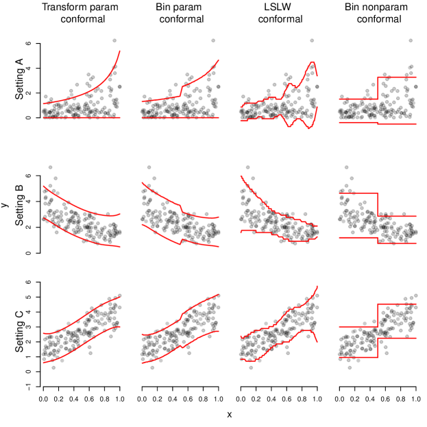
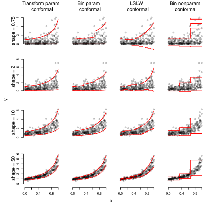
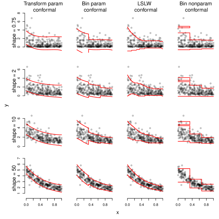
The prediction regions under consideration are the transformation based parametric, binned parametric, binned nonparametric, LSLW, and LS conformal prediction regions and the highest density (HD) prediction region under an assumed model. The transformation based parametric, binned parametric, and binned nonparametric are fit using the conformal.glm R package (Eck, 2018) with default settings employed which specifies line search precision at 0.005. The LSLW and LS are fit using the conformalInference R package (Tibshirani, 2016) with the default settings employed which specifies that the number of grid points is 100. The HD prediction region is fit using using the HDInterval R package (Meredith and Kruschke, 2018). Following the bin width asymptotics of Lei and Wasserman (2014), the number of bins used to form the binned parametric and nonparametric conformal prediction regions is 2 when n=150𝑛150n=150 and 3 when n=250,500𝑛250500n=250,500. All simulations correspond to univariate regressions and the predictor variables were generated as XU(0,1)similar-to𝑋𝑈01X\sim U(0,1). Figure 2 shows four example conformal regions for simulation setting A, B, and C with n=150𝑛150n=150.

Refer to caption
Figure 2: Illustration of conformal prediction regions. The top, middle, and bottom rows correspond to simulation setting A with shape parameter equal to 1, simulation setting B with shape parameter equal to 10, and simulation setting C respectively. The first column depicts the transformation based parametric conformal prediction region which is misspecified in row 2. The second column depicts the binned parametric conformal prediction region which is misspecified in row 2. The third column depicts the locally weighted conformal prediction region. The fourth column depicts the nonparametric conformal prediction region.

Several diagnostic measures are used to compare conformal prediction regions. These diagnostic measures compare prediction regions by their prediction error, volume, and coverage properties. Our prediction error diagnostic metric will be an average of the squared distances of observations outside of the prediction region to the closest boundary of the prediction region, averaged over all observations. An observation that falls within the prediction region has an error of 0. More formally this prediction error metric is

prediction error=n1i=1n𝟙{YiC(α)(Xi)}(minj=1,,mi{min{|Yiai,j|,|Yibi,j|}})2,prediction errorsuperscript𝑛1superscriptsubscript𝑖1𝑛1subscript𝑌𝑖superscript𝐶𝛼subscript𝑋𝑖superscriptsubscript𝑗1subscript𝑚𝑖subscript𝑌𝑖subscript𝑎𝑖𝑗subscript𝑌𝑖subscript𝑏𝑖𝑗2\text{prediction error}=n^{-1}\sum_{i=1}^{n}\mathds{1}\left\{Y_{i}\not\in C^{(\alpha)}(X_{i})\right\}\left(\min_{j=1,\ldots,m_{i}}\left\{\min\{|Y_{i}-a_{i,j}|,|Y_{i}-b_{i,j}|\}\right\}\right)^{2},

where ai,jsubscript𝑎𝑖𝑗a_{i,j} and bi,jsubscript𝑏𝑖𝑗b_{i,j} are, respectively, the lower and upper boundaries of possible j=1,,mi𝑗1subscript𝑚𝑖j=1,\ldots,m_{i} disjoint intervals forming the prediction region.

The volume of each prediction region will be estimated by the average of the upper boundary minus the lower boundary across observed 𝒳𝒳\mathcal{X}, written as

area=n1i=1nj=1mi(bi,jai,j).areasuperscript𝑛1superscriptsubscript𝑖1𝑛superscriptsubscript𝑗1subscript𝑚𝑖subscript𝑏𝑖𝑗subscript𝑎𝑖𝑗\text{area}=n^{-1}\sum_{i=1}^{n}\sum_{j=1}^{m_{i}}(b_{i,j}-a_{i,j}).

To assess finite sample marginal validity we calculate the proportion of responses that fall within the prediction region. To assess finite sample local validity with respect to binning we first bin the predictor data and then, for each bin, we calculate the proportion of responses that fall within the prediction region. The same procedure is used to assess finite sample conditional validity, but we use a much finer binning regime than what was used to assess finite sample local validity.
Refer to caption
Refer to caption
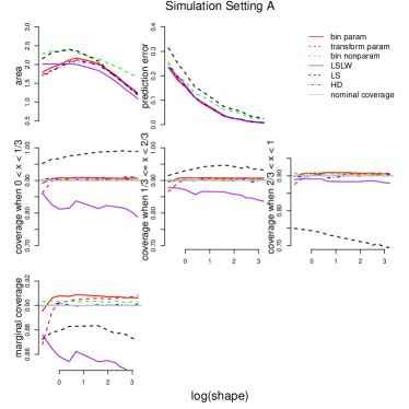
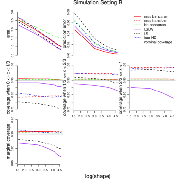
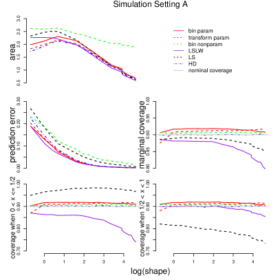
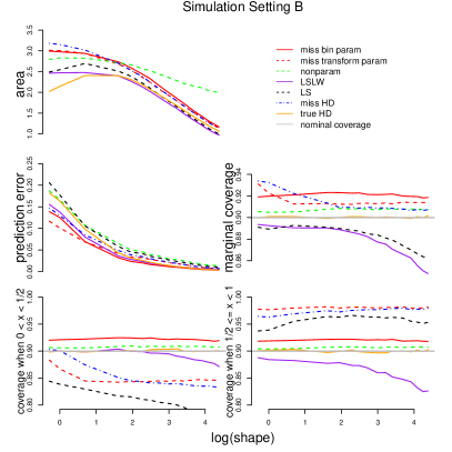
Figure 3: Area, prediction error, and bin-wise coverage for parametric, nonparametric, LS, LSLW conformal prediction region, and the highest density prediction region for Gamma GLM regression with n=150𝑛150n=150 and α=0.1𝛼0.1\alpha=0.1. Simulation setting A is shown at left, and setting B at right. The average of 250 samples at each shape parameter value in these simulation settings form the lines that are depicted in both plots of this figure.

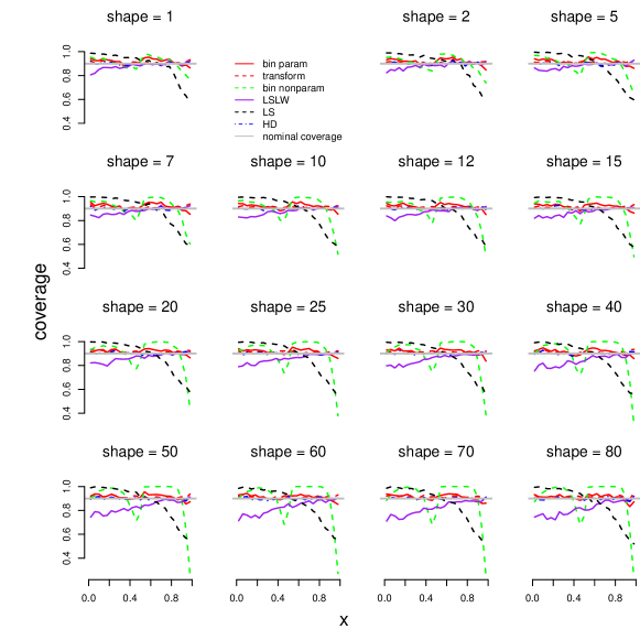
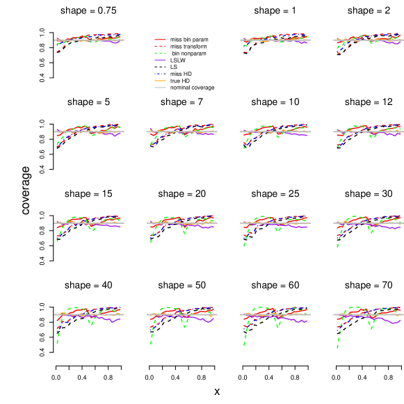
In our simulations, we find that the parametric conformal prediction regions perform well even when the model is moderately misspecified. By construction, the binned parametric conformal prediction region, along with the binned nonparametric conformal prediction region, maintains finite sample local validity with respect to binning as seen in the bottom row of both plots in Figure 3 and Table 1. However, these prediction regions have different shapes conditional on x𝑥x, as seen in Figure 2, and give different prediction errors as seen in the top row of both plots in Figure 3 and Table 1. Both parametric conformal prediction regions adapt naturally to the data when the model is correctly specified or when modest deviations from the specified model are present. However, large deviations from model misspecification are not handled well as seen in the top row of the right hand side of Figure 3, although the transformation and binned parametric conformal prediction region give nominal marginal and local coverage respectively as seen in the middle row in the right hand side of Figure 3. Note that the default precision allowed the transformation based parametric conformal prediction region to exhibits undercoverage for small values of x𝑥x, and note overcoverage for large values of x𝑥x in the bottom row of the right hand side of Figure 3. On the other hand, the nonparametric conformal prediction region does not adapt well to data obtained from a Gamma regression model, and the former is not data adaptive in our linear regression setting.

OLS trans OLS bin bin nonparametric LS LSLW HD
conformal conformal conformal conformal conformal region
n=150𝑛150n=150 marginal coverage 0.9110.9110.911 0.9190.9190.919 0.9110.9110.911 0.8780.8780.878 0.8830.8830.883 0.9040.9040.904
local coverage when 0<x<1/20𝑥120<x<1/2 0.9120.9120.912 0.9180.9180.918 0.9110.9110.911 0.8780.8780.878 0.8860.8860.886 0.9030.9030.903
local coverage when 1/2x<112𝑥11/2\leq x<1 0.9090.9090.909 0.920.920.92 0.9110.9110.911 0.8780.8780.878 0.8810.8810.881 0.9040.9040.904
area 1.881.881.88 1.9941.9941.994 2.4082.4082.408 1.7751.7751.775 1.7821.7821.782 1.8721.8721.872
prediction error 0.010.010.01 0.0070.0070.007 0.0110.0110.011 0.0120.0120.012 0.0110.0110.011 0.010.010.01
n=250𝑛250n=250 marginal coverage 0.9080.9080.908 0.9160.9160.916 0.9090.9090.909 0.8750.8750.875 0.8780.8780.878 0.9020.9020.902
local coverage when 0<x<1/30𝑥130<x<1/3 0.90.90.9 0.9160.9160.916 0.9090.9090.909 0.870.870.87 0.8820.8820.882 0.8960.8960.896
local coverage when 1/3x<2/313𝑥231/3\leq x<2/3 0.9140.9140.914 0.9130.9130.913 0.9090.9090.909 0.8790.8790.879 0.8760.8760.876 0.9070.9070.907
local coverage when 2/3x<123𝑥12/3\leq x<1 0.9090.9090.909 0.920.920.92 0.9090.9090.909 0.8770.8770.877 0.8760.8760.876 0.9040.9040.904
area 1.8771.8771.877 1.9741.9741.974 2.1392.1392.139 1.7511.7511.751 1.7541.7541.754 1.8641.8641.864
prediction error 0.0090.0090.009 0.0070.0070.007 0.010.010.01 0.0130.0130.013 0.0120.0120.012 0.010.010.01
n=500𝑛500n=500 marginal coverage 0.9080.9080.908 0.9070.9070.907 0.9040.9040.904 0.8750.8750.875 0.8730.8730.873 0.9020.9020.902
local coverage when 0<x<1/30𝑥130<x<1/3 0.9110.9110.911 0.9080.9080.908 0.9060.9060.906 0.8780.8780.878 0.8750.8750.875 0.9050.9050.905
local coverage when 1/3x<2/313𝑥231/3\leq x<2/3 0.9070.9070.907 0.9070.9070.907 0.9040.9040.904 0.8740.8740.874 0.8710.8710.871 0.9020.9020.902
local coverage when 2/3x<123𝑥12/3\leq x<1 0.9050.9050.905 0.9070.9070.907 0.9040.9040.904 0.8740.8740.874 0.8750.8750.875 0.8990.8990.899
area 1.8861.8861.886 1.9041.9041.904 2.0982.0982.098 1.7351.7351.735 1.7311.7311.731 1.861.861.86
prediction error 0.0090.0090.009 0.0090.0090.009 0.0110.0110.011 0.0130.0130.013 0.0130.0130.013 0.010.010.01
Table 1: Diagnostics for conformal prediction regions for linear regression models with normal errors and constant variance. Local and marginal coverage properties, areas, and prediction errors are presented for the transformation based and binned parametric conformal prediction regions, binned nonparametric conformal prediction region, LS conformal prediction region, LSLW conformal prediction region, and HD prediction region.

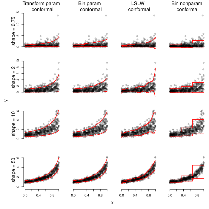
The LS conformal prediction region obtains marginal validity (Lei et al., 2018) but performs poorly when deviations about the estimated mean function are either not symmetric, not constant, or both. When heterogeneity is present, the LS conformal prediction region exhibits undercoverage in regions where variability about the mean function is large and over-coverage in regions where variability about the mean function is small. Clear evidence of these features are seen in Figure 3 and 2. This conformal prediction region is very sensitive to model misspecification. The LSLW conformal prediction region also guarantees marginal validity (Lei et al., 2018, Section 5.2), although our simulations reveal that the default software implementation struggles to guarantee this in practice. That being said, the LSLW region appears to exhibit flexibility under mild model misspecification as evidenced in the second row of Figure 2 and our Supplementary Materials. This region is far less sensitive to model misspecification than the LS conformal prediction region, and it performs well under modest model misspecification. However, the LSLW conformal prediction region is not appropriate when deviations about an estimated mean function are obviously not symmetric, as evidenced in the top row of Figure 2. Results from additional simulations corresponding to settings A and B are provided in the Supplementary Materials. The findings from these additional simulations are consistent with the conclusions of the simulations presented in this Section.

6 Predicting the risk of diabetes
Refer to caption
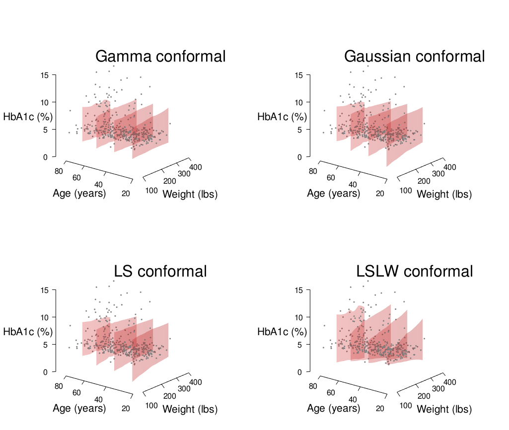
Figure 4: Conformal prediction regions for glycosylated hemoglobin projected onto the age and weight predictor axes. Upper and lower bounds of the conformal prediction region are loess smoothed for visual appearance.

Diabetes is a group of metabolic diseases associated with long-term damage, dysfunction, and failure of different organs, especially the eyes, kidneys, nerves, heart, and blood vessels (American Diabetes Association, 2010). In 2017 approximately 5 million adult deaths worldwide were attributable to diabetes; global healthcare expenditures on people with diabetes are estimated USD 850 billion (Cho et al., 2018). Diabetes remains undiagnosed for an estimated 30% of the people who have the disease (Heikes et al., 2008). One way to address the problem of undiagnosed diabetes is to develop simple, inexpensive diagnostic tools that can identify people who are at high risk of pre-diabetes or diabetes using only readily-available clinical or demographic information (Heikes et al., 2008).

We examine the influence of several variables on blood sugar, or glycosylated hemoglobin percentage (also known as HbA1c), an important risk factor for diabetes. A glycosylated hemoglobin value of 6.5% can be used as a cutoff for positive diagnosis of diabetes (World Health Organization, 2011). We predict an individual’s glycosylated hemoglobin from their height, weight, age, and gender, all of which are easy to measure, inexpensive, and do not require any laboratory testing. The data in this analysis come from a population-based sample of 403 rural African-Americans in Virginia (Willems et al., 1997), taken from the faraway R package (Faraway, 2016). We considered a gamma regression model that only includes linear terms for each covariate, a linear regression model with homoskedastic normal errors and the same linear terms for each covariate, and a linear regression model with homoskedastic normal errors that also included quadratic terms for each covariate. Of these considered models, the gamma regression model fit the data best: it had the lowest AIC value and gives the best predictive predictive performance as measured by the sum of squares prediction error.

Based on these covariates, conformal prediction regions provide finite sample valid prediction regions for glycosylated hemoglobin that may be useful for diagnosing diabetes in this study population. Six conformal prediction regions are considered for predicting glycosylated hemoglobin percentage. These conformal prediction regions are the binned and transformation parametric conformal prediction region with a Gamma model fit, the binned and transformation parametric conformal prediction region with a Gaussian model fit, the LS conformal prediction region, and the LSLW conformal prediction region. All conformal prediction regions correspond to models that only include linear terms for each of the covariates. The binned Gamma and Gaussian parametric conformal prediction regions were computed with binning across the binary gender factor variable, the predictor space is partitioned across genders. However, no additional binning structure within the levels of gender was employed.

Gamma trans Gaussian trans Gamma bin Gaussian bin LSLW LS
conformal conformal conformal conformal conformal conformal
marginal coverage 0.901 0.924 0.909 0.906 0.880 0.888
volume 7.656 8.560 7.349 7.730 8.574 7.103
pred error 0.653 0.425 0.931 0.849 0.803 1.012
avg.cond.coverage 0.856 0.888 0.874 0.849 0.863 0.827
Table 2: Diagnostics for prediction regions. Marginal coverage (α=0.10𝛼0.10\alpha=0.10), prediction region volume, prediction error, and average conditional coverage make up the first four rows.

Diagnostics from the six conformal prediction regions are depicted in Table 2. The error tolerance for all prediction regions was set at α=0.10𝛼0.10\alpha=0.10. We see that parametric conformal prediction regions maintain their advertised finite sample marginal validity for the predictions of glycosylated hemoglobin. These prediction regions provide a balance between marginal coverage, size, prediction error, and average conditional coverage (the average of the coverage probabilities taken over small subregions of the predictor space). The transformation Gamma conformal prediction region balances these criteria particularly nicely. This prediction region is relatively small, has relatively small prediction error, and it gives near nominal desired coverage. This finding is expected when the underlying estimated density used as the parametric conformity measure is a good approximation of the data generating model.

Plots of three dimensional conformal prediction region are displayed in Figure 4. These plots are projections of each conformal prediction regions to the age (in years), weight (in pounds), and glycosylated hemoglobin percentage three dimensional space.

7 Discussion

The finite sample validity properties of conformal prediction regions have been verified in broader methodological contexts, including support vector machines, ridge regression, nearest neighbor regression, neural networks, and decision decision trees (Vovk et al., 2005; Gammerman and Vovk, 2007; Papadopoulos et al., 2011; Vovk, 2012). While any conformity measure function will achieve finite sample validity, a careful choice may make the returned conformal prediction regions more useful in applications (Papadopoulos et al., 2011). The developments of conformal prediction in the machine learning literature show how empirically successful prediction methods in machine learning can be hedged to give valid predictions in finite samples (Gammerman and Vovk, 2007). The developments of conformal prediction in the statistics literature show that specification of the conformity measure to incorporate knowledge about the data generating process can lead to conformal prediction regions which are also asymptotically of minimal length (Lei and Wasserman, 2014; Dunn and Wasserman, 2018). Our parametric conformal prediction regions for parametric regression models falls within this line of research, which addresses efficiency concerns of conformal prediction methodology raised by Cortés-Ciriano and Bender (2019). This line of research shows that when uncertainty about point predictions is considered, regression modeling provides smaller prediction regions when we require regions to guarantee valid finite sample coverage.

Because GLMs are widely used by empiricists conducting regression analyses, parametric conformal prediction for GLM regression therefore may offer an appealing compromise for the applied researcher: when the GLM is correctly specified, conformal prediction regions are asymptotically minimal, finite sample local and marginal validity holds, and the rate of convergence is fast; when the GLM is incorrectly specified, asymptotic minimality is not guaranteed, but local finite sample validity still holds by construction. Researchers who currently use GLMs to compute prediction intervals for the mean regression function may be able to easily integrate conformal prediction into their data analysis workflow, since specification and fitting of the GLM is unchanged. A software package that accompanies this paper implements the parametric and nonparametric conformal prediction regions (Eck, 2018).

The robustness properties of conformal prediction come at a substantial computational cost (Vovk, 2012). In our software implementation of the conformal methodology, two line searches are performed to determine the boundaries of the possibly disjoint conformal prediction region at every point at which a prediction region is desired. The conformity scores must be recomputed with respect to augmented data at every iteration of these line searches. This involves refitting the parametric model to augmented data at every iteration of the line search to construct the parametric conformal prediction region. Furthermore, when sample sizes are very large, conformal prediction may not offer much additional benefit beyond the parametric conditional prediction regions available in popular software packages for regression. However, when sample sizes are moderate, conformal prediction may substantially outperform traditional methods in terms of finite sample marginal, local, and conditional coverage.

The asymptotic optimality properties of parametric conformal prediction regions follow from our concentration inequality for maximum likelihood estimation stated in Theorem 4. We conjecture that a similar concentration inequality may hold for random variables whose score functions do not have functional subexponential behavior (see Appendix), and/or a non-existent MGF. This concentration inequality will likely induce convergence rates that are slower than log(n)/n𝑛𝑛\sqrt{\log(n)/n}. Dunn and Wasserman (2018) showed that finite sample validity holds in the presence of random effects. We expect that asymptotic optimality properties for parametric conformal prediction regions can be extended to their settings and to the class of generalized linear mixed models.

Supplementary Materials: Additional simulation results are available in the accompanying Supplementary Materials document (appended at the end of the main text). An accompanying R package is available at https://github.com/DEck13/conformal.glm (Eck, 2018). A technical report that includes the data and all of the code necessary to reproduce the findings, tables, and figures in this manuscript is available at https://github.com/DEck13/conformal.glm/tree/master/techreport.

Acknowledgments: We are grateful to Peter M. Aronow, Karl Oskar Ekvall, Jing Lei, Aaron J. Molstad, Molly Offer-Westort, Cyrus Samii, Fredrik Sävje, and Larry Wasserman for helpful comments. This work was supported by NIH grant NICHD 1DP2HD091799-01.

Appendix: Mathematical details

Subexponential random variables

The following definition and two lemmas are taken from Wainwright (2019, Chapter 2).

Definition 4.

A mean zero random variable Y𝑌Y is said to be subexponential with parameters (τ2,b)superscript𝜏2𝑏(\tau^{2},b) if 𝔼{exp(tY)}exp(t2τ2/2)𝔼𝑡𝑌superscript𝑡2superscript𝜏22\mathbb{E}\left\{\exp(tY)\right\}\leq\exp\left(t^{2}\tau^{2}/2\right) for all |t|1/b𝑡1𝑏|t|\leq 1/b.

Lemma 5.

For a mean zero random variable Y𝑌Y, the following are equivalent: (a) Y𝑌Y is subexponential with parameters (τ2,b)superscript𝜏2𝑏(\tau^{2},b); (b) There is a positive number c0>0subscript𝑐00c_{0}>0 such that 𝔼(etY)<𝔼superscript𝑒𝑡𝑌\mathbb{E}\left(e^{tY}\right)<\infty for all |t|<c0𝑡subscript𝑐0|t|<c_{0}; (c) {Y𝔼(Y)+t}max(et22τ2,et2b).𝑌𝔼𝑌𝑡superscript𝑒superscript𝑡22superscript𝜏2superscript𝑒𝑡2𝑏\mathbb{P}\left\{Y\geq\mathbb{E}(Y)+t\right\}\leq\max\left(e^{-\frac{t^{2}}{2\tau^{2}}},e^{-\frac{t}{2b}}\right).

Lemma 6.

Let Yisubscript𝑌𝑖Y_{i} be independent mean zero subexponential random variables with parameters (τi2,bi)superscriptsubscript𝜏𝑖2subscript𝑏𝑖(\tau_{i}^{2},b_{i}). Then i=1nYisuperscriptsubscript𝑖1𝑛subscript𝑌𝑖\sum_{i=1}^{n}Y_{i} is subexponential with parameters (i=1nτi2,b)superscriptsubscript𝑖1𝑛superscriptsubscript𝜏𝑖2subscript𝑏\left(\sum_{i=1}^{n}\tau_{i}^{2},b_{\star}\right) where b=maxi(bi)subscript𝑏subscript𝑖subscript𝑏𝑖b_{\star}=\max_{i}(b_{i}) and

{|1ni=1nYi|t}2exp{min(nt22n1i=1nτi2,nt2b)}.1𝑛superscriptsubscript𝑖1𝑛subscript𝑌𝑖𝑡2𝑛superscript𝑡22superscript𝑛1superscriptsubscript𝑖1𝑛superscriptsubscript𝜏𝑖2𝑛𝑡2subscript𝑏\mathbb{P}\left\{\left|\frac{1}{n}\sum_{i=1}^{n}Y_{i}\right|\geq t\right\}\leq 2\exp\left\{-\min\left(\frac{nt^{2}}{2n^{-1}\sum_{i=1}^{n}\tau_{i}^{2}},\frac{nt}{2b_{\star}}\right)\right\}. (13)

Let lψ(Y|x)=logpψ(Y|x)subscript𝑙𝜓conditional𝑌𝑥subscript𝑝𝜓conditional𝑌𝑥l_{\psi}(Y|x)=\log p_{\psi}(Y|x) be the log likelihood for the random variable Y|X=xconditional𝑌𝑋𝑥Y|X=x and let ψlψ(Y|x)subscript𝜓subscript𝑙𝜓conditional𝑌𝑥\nabla_{\psi}l_{\psi}(Y|x) be the corresponding score function. We will now motivate the construction of the parameter space 𝒳subscript𝒳\aleph_{\mathcal{X}}. This parameter space requires a notion of functional subexponential that we will now define and examine.

Definition 5 (functional subexponential).

Let Y𝑌Y be a random variable and suppose that f::𝑓f:\mathbb{R}\to\mathbb{R} is a function such that E{f(Y)}=0𝐸𝑓𝑌0E\{f(Y)\}=0. We say that f𝑓f is functional subexponential with respect to Y𝑌Y with parameters (τ2,b)superscript𝜏2𝑏(\tau^{2},b) if 𝔼{exp(tf(Y))}exp(t2τ2/2)𝔼𝑡𝑓𝑌superscript𝑡2superscript𝜏22\mathbb{E}\left\{\exp(tf(Y))\right\}\leq\exp\left(t^{2}\tau^{2}/2\right) for all |t|1/b𝑡1𝑏|t|\leq 1/b.

Definition 6 (multivariate functional subexponential).

Let Y𝑌Y be a random variable and suppose that f:r:𝑓superscript𝑟f:\mathbb{R}\to\mathbb{R}^{r} is a function such that E{f(Y)}=0𝐸𝑓𝑌0E\{f(Y)\}=0. We say that f𝑓f is multivariate functional subexponential with respect to Y𝑌Y with parameters (τ2,b)superscript𝜏2𝑏(\tau^{2},b) if 𝔼{exp(tf(Y))}exp(|t|2τ2/2)𝔼superscript𝑡𝑓𝑌superscript𝑡2superscript𝜏22\mathbb{E}\left\{\exp(t^{\prime}f(Y))\right\}\leq\exp\left(|t|^{2}\tau^{2}/2\right) for all |t|1/b𝑡1𝑏|t|\leq 1/b.

Lemma 7.

Let Y𝑌Y be a random variable and suppose that f:r:𝑓superscript𝑟f:\mathbb{R}\to\mathbb{R}^{r} is a function such that E{f(Y)}=0𝐸𝑓𝑌0E\{f(Y)\}=0. Then f(Y)𝑓𝑌f(Y) is multivariate functional subexponential with respect to Y𝑌Y if and only the components of f(Y)𝑓𝑌f(Y) are functional subexponential with respect to Y𝑌Y.

Proof.

First suppose that f(Y)𝑓𝑌f(Y) is multivariate functional subexponential with respect to Y𝑌Y. Let sjsubscript𝑠𝑗s_{j} be the r𝑟r dimensional zeros vector with an s𝑠s in the j𝑗jth component. Then 𝔼{exp(sfj(Y))}exp(s2τ2/2)𝔼𝑠subscript𝑓𝑗𝑌superscript𝑠2superscript𝜏22\mathbb{E}\left\{\exp(sf_{j}(Y))\right\}\leq\exp\left(s^{2}\tau^{2}/2\right) for all |s|1/b𝑠1𝑏|s|\leq 1/b where fj(Y)subscript𝑓𝑗𝑌f_{j}(Y) is the j𝑗jth component of f(Y)𝑓𝑌f(Y). It follows that the components of f(Y)𝑓𝑌f(Y) are functional subexponential with respect to Y𝑌Y.

Now suppose that the components of f(Y)𝑓𝑌f(Y) are functional subexponential with respect to Y𝑌Y with parameters (τj2,bj)subscriptsuperscript𝜏2𝑗subscript𝑏𝑗(\tau^{2}_{j},b_{j}), j=1,,r𝑗1𝑟j=1,...,r. Let b=max(bj)𝑏subscript𝑏𝑗b=\max(b_{j}) and τ=max(τj)𝜏subscript𝜏𝑗\tau=\max(\tau_{j}). Then 𝔼{exp(sfj(Y))}exp(s2τ2/2)𝔼𝑠subscript𝑓𝑗𝑌superscript𝑠2superscript𝜏22\mathbb{E}\left\{\exp(sf_{j}(Y))\right\}\leq\exp\left(s^{2}\tau^{2}/2\right) holds for all |s|1/b𝑠1𝑏|s|\leq 1/b. Now pick a vector tr𝑡superscript𝑟t\in\mathbb{R}^{r} such that |t|<1/b𝑡1𝑏|t|<1/b. Then by multiple applications of Cauchy Scharwz and the supposition that the components of f(Y)𝑓𝑌f(Y) are functional subexponential we have that

𝔼{exp(tf(Y))}=𝔼{j=1rexp(tjfj(Y))}j=1r𝔼{exp(2jtjfj(Y))}1/2j𝔼superscript𝑡𝑓𝑌𝔼superscriptsubscriptproduct𝑗1𝑟subscript𝑡𝑗subscript𝑓𝑗𝑌superscriptsubscriptproduct𝑗1𝑟𝔼superscriptsuperscript2𝑗subscript𝑡𝑗subscript𝑓𝑗𝑌1superscript2𝑗\displaystyle\mathbb{E}\left\{\exp(t^{\prime}f(Y))\right\}=\mathbb{E}\left\{\prod_{j=1}^{r}\exp(t_{j}f_{j}(Y))\right\}\leq\prod_{j=1}^{r}\mathbb{E}\left\{\exp(2^{j}t_{j}f_{j}(Y))\right\}^{1/2^{j}}
j=1r𝔼{exp(22j1tj2τ2)}1/2jj=1r𝔼{exp(2jtj2τ2/2)}exp(|t|22rτ22),absentsuperscriptsubscriptproduct𝑗1𝑟𝔼superscriptsuperscript22𝑗1superscriptsubscript𝑡𝑗2superscript𝜏21superscript2𝑗superscriptsubscriptproduct𝑗1𝑟𝔼superscript2𝑗superscriptsubscript𝑡𝑗2superscript𝜏22superscript𝑡2superscript2𝑟superscript𝜏22\displaystyle\qquad\leq\prod_{j=1}^{r}\mathbb{E}\left\{\exp(2^{2j-1}t_{j}^{2}\tau^{2})\right\}^{1/2^{j}}\leq\prod_{j=1}^{r}\mathbb{E}\left\{\exp(2^{j}t_{j}^{2}\tau^{2}/2)\right\}\leq\exp\left(\frac{|t|^{2}2^{r}\tau^{2}}{2}\right),

for all |t|<1/b𝑡1𝑏|t|<1/b. Set τ=τ2r/2superscript𝜏𝜏superscript2𝑟2\tau^{\prime}=\tau 2^{r/2}, then f(Y)𝑓𝑌f(Y) is multivariate subexponential with respect to Y𝑌Y with parameters (τ,b)superscript𝜏𝑏(\tau^{\prime},b). The conclusion follows. ∎

The following Lemma is the key piece that ties 𝒳subscript𝒳\aleph_{\mathcal{X}} together with the concentration inequality given in Theorem 4.

Lemma 8.

Let Y|X=xconditional𝑌𝑋𝑥Y|X=x be a random variable and suppose that the moment generating function MY,x,ψ(t)subscript𝑀𝑌𝑥𝜓𝑡M_{Y,x,\psi}(t) exists for all t𝑡t in a neighborhood of 00. Let pψ(y|x)subscript𝑝𝜓conditional𝑦𝑥p_{\psi}(y|x) be the corresponding probability density function with parameter vector ψr𝜓superscript𝑟\psi\in\mathbb{R}^{r}. Assume that pψ(y|x)subscript𝑝𝜓conditional𝑦𝑥p_{\psi}(y|x) is differentiable in both y𝑦y and ψ𝜓\psi. Then the score function ψlogpψ(Y|x)subscript𝜓subscript𝑝𝜓conditional𝑌𝑥\nabla_{\psi}\log p_{\psi}(Y|x) is functional subexponential with respect to Y|X=xconditional𝑌𝑋𝑥Y|X=x provided that ψlogpψ(y|x)=O(y)subscript𝜓subscript𝑝𝜓conditional𝑦𝑥𝑂𝑦\nabla_{\psi}\log p_{\psi}(y|x)=O(y).

Proof.

Let ψjlogpψ(y|x)subscriptsubscript𝜓𝑗subscript𝑝𝜓conditional𝑦𝑥\nabla_{\psi_{j}}\log p_{\psi}(y|x) be the j𝑗jth component of ψlogpψ(y|x)subscript𝜓subscript𝑝𝜓conditional𝑦𝑥\nabla_{\psi}\log p_{\psi}(y|x). Then,

𝔼{exp(tjψjlogpψ(Y|x))}=exp(tjψjlogpψ(y))pψ(y|x)𝑑y𝔼subscript𝑡𝑗subscriptsubscript𝜓𝑗subscript𝑝𝜓conditional𝑌𝑥subscript𝑡𝑗subscriptsubscript𝜓𝑗subscript𝑝𝜓𝑦subscript𝑝𝜓conditional𝑦𝑥differential-d𝑦\displaystyle\mathbb{E}\{\exp(t_{j}\nabla_{\psi_{j}}\log p_{\psi}(Y|x))\}=\int\exp(t_{j}\nabla_{\psi_{j}}\log p_{\psi}(y))p_{\psi}(y|x)dy
=exp{tjy(ψjlogpψ(y|x)y)}pψ(y|x)𝑑y<,absentsubscript𝑡𝑗𝑦subscriptsubscript𝜓𝑗subscript𝑝𝜓conditional𝑦𝑥𝑦subscript𝑝𝜓conditional𝑦𝑥differential-d𝑦\displaystyle\qquad=\int\exp\left\{t_{j}y\left(\frac{\nabla_{\psi_{j}}\log p_{\psi}(y|x)}{y}\right)\right\}p_{\psi}(y|x)dy<\infty,

for all tjsubscript𝑡𝑗t_{j} in a neighborhood about 00, and all j=1𝑗1j=1, \ldots, r𝑟r. The same argument as that in Appendix B of Wainwright (2019) implies that the score function ψjlogpψ(Y)subscriptsubscript𝜓𝑗subscript𝑝𝜓𝑌\nabla_{\psi_{j}}\log p_{\psi}(Y) is functional subexponential with respect to Y|X=xconditional𝑌𝑋𝑥Y|X=x. Our conclusion follows from Lemma 7. ∎

Conentration results

We can now prove Theorem 4 from Lemma 8 and our developed notion of functional subexponential random variables.

Proof of Theorem 4.

From the mean-value theorem, there exists some ψ^1subscript^𝜓1\hat{\psi}_{1} such that ψ^1,j(ψjψ^j\hat{\psi}_{1,j}\in(\psi_{j}\wedge\hat{\psi}_{j}, ψjψ^j)\psi_{j}\vee\hat{\psi}_{j}), j=1𝑗1j=1, \ldots, r𝑟r, which satisfies

ψln(ψ)=ψ2ln(ψ^1)(ψ^ψ).subscript𝜓subscript𝑙𝑛𝜓superscriptsubscript𝜓2subscript𝑙𝑛subscript^𝜓1^𝜓𝜓-\nabla_{\psi}l_{n}(\psi)=\nabla_{\psi}^{2}l_{n}(\hat{\psi}_{1})(\hat{\psi}-\psi).

Rearranging the above yields

n(ψ^ψ)=n{ψ2ln(ψ^1)}1ψln(ψ)𝑛^𝜓𝜓𝑛superscriptsuperscriptsubscript𝜓2subscript𝑙𝑛subscript^𝜓11subscript𝜓subscript𝑙𝑛𝜓\sqrt{n}(\hat{\psi}-\psi)=-\sqrt{n}\left\{\nabla_{\psi}^{2}l_{n}(\hat{\psi}_{1})\right\}^{-1}\nabla_{\psi}l_{n}(\psi)

where the inverse exists almost surely when n>r𝑛𝑟n>r. We see that

|n(ψ^ψ)|𝑛^𝜓𝜓\displaystyle\left|\sqrt{n}(\hat{\psi}-\psi)\right| =|n{ψ2ln(ψ^1)}1ψln(ψ)|absent𝑛superscriptsuperscriptsubscript𝜓2subscript𝑙𝑛subscript^𝜓11subscript𝜓subscript𝑙𝑛𝜓\displaystyle=\left|\sqrt{n}\left\{\nabla_{\psi}^{2}l_{n}(\hat{\psi}_{1})\right\}^{-1}\nabla_{\psi}l_{n}(\psi)\right|
|n{ψ2ln(ψ)}1ψln(ψ)|+|an|absent𝑛superscriptsuperscriptsubscript𝜓2subscript𝑙𝑛𝜓1subscript𝜓subscript𝑙𝑛𝜓subscript𝑎𝑛\displaystyle\leq\left|\sqrt{n}\left\{\nabla_{\psi}^{2}l_{n}(\psi)\right\}^{-1}\nabla_{\psi}l_{n}(\psi)\right|+|a_{n}|
n{ψ2ln(ψ)}11|ψln(ψ)|+|an|,absent𝑛subscriptnormsuperscriptsuperscriptsubscript𝜓2subscript𝑙𝑛𝜓11subscript𝜓subscript𝑙𝑛𝜓subscript𝑎𝑛\displaystyle\leq\sqrt{n}\left\|\left\{\nabla_{\psi}^{2}l_{n}(\psi)\right\}^{-1}\right\|_{1}\left|\nabla_{\psi}l_{n}(\psi)\right|+|a_{n}|,

where 1\|\cdot\|_{1} is the induced k𝑘k-norm for a matrix with k=1𝑘1k=1 and

|an|=|n[{ψ2ln(ψ^1)}1{ψ2ln(ψ)}1]ψln(ψ)|.subscript𝑎𝑛𝑛delimited-[]superscriptsuperscriptsubscript𝜓2subscript𝑙𝑛subscript^𝜓11superscriptsuperscriptsubscript𝜓2subscript𝑙𝑛𝜓1subscript𝜓subscript𝑙𝑛𝜓|a_{n}|=\left|\sqrt{n}\left[\left\{\nabla_{\psi}^{2}l_{n}(\hat{\psi}_{1})\right\}^{-1}-\left\{\nabla_{\psi}^{2}l_{n}(\psi)\right\}^{-1}\right]\nabla_{\psi}l_{n}(\psi)\right|.

Choose some 0<aλ<Aλ0subscript𝑎𝜆subscript𝐴𝜆0<a_{\lambda}<A_{\lambda} and let Bλ=Aλaλsubscript𝐵𝜆subscript𝐴𝜆subscript𝑎𝜆B_{\lambda}=A_{\lambda}-a_{\lambda}. Then for n𝑛n sufficiently large,

{n|ψ^ψ|Aλlog(n)}{n{ψ2ln(ψ)}11|ψln(ψ)|+|an|Aλlog(n)}𝑛^𝜓𝜓subscript𝐴𝜆𝑛conditional-set𝑛evaluated-atsuperscriptsuperscriptsubscript𝜓2subscript𝑙𝑛𝜓11subscript𝜓subscript𝑙𝑛𝜓subscript𝑎𝑛subscript𝐴𝜆𝑛\displaystyle\mathbb{P}\left\{\sqrt{n}\left|\hat{\psi}-\psi\right|\geq A_{\lambda}\sqrt{\log(n)}\right\}\leq\mathbb{P}\left\{\sqrt{n}\left\|\left\{\nabla_{\psi}^{2}l_{n}(\psi)\right\}^{-1}\right\|_{1}\left|\nabla_{\psi}l_{n}(\psi)\right|+|a_{n}|\geq A_{\lambda}\sqrt{\log(n)}\right\}
(|ψln(ψ)|log(n)nBλ{ψ2ln(ψ)}11)absentsubscript𝜓subscript𝑙𝑛𝜓𝑛𝑛subscript𝐵𝜆subscriptnormsuperscriptsuperscriptsubscript𝜓2subscript𝑙𝑛𝜓11\displaystyle\qquad\leq\mathbb{P}\left(\left|\nabla_{\psi}l_{n}(\psi)\right|\geq\sqrt{\frac{\log(n)}{n}}\frac{B_{\lambda}}{\left\|\left\{\nabla_{\psi}^{2}l_{n}(\psi)\right\}^{-1}\right\|_{1}}\right)
=(|n1i=1nψli(ψ)|log(n)nBλn1{ψ2ln(ψ)}11),absentsuperscript𝑛1superscriptsubscript𝑖1𝑛subscript𝜓subscript𝑙𝑖𝜓𝑛𝑛subscript𝐵𝜆subscriptnormsuperscript𝑛1superscriptsuperscriptsubscript𝜓2subscript𝑙𝑛𝜓11\displaystyle\qquad=\mathbb{P}\left(\left|n^{-1}\sum_{i=1}^{n}\nabla_{\psi}l_{i}(\psi)\right|\geq\sqrt{\frac{\log(n)}{n}}\frac{B_{\lambda}}{\left\|n^{-1}\left\{\nabla_{\psi}^{2}l_{n}(\psi)\right\}^{-1}\right\|_{1}}\right),

where the second inequality follows from the strong law of large numbers with respect to ansubscript𝑎𝑛a_{n} and li(ψ)subscript𝑙𝑖𝜓l_{i}(\psi) is the log likelihood for each observation. We can now choose some D>𝔼[{ψ2ln=1(ψ)}1]1𝐷subscriptnorm𝔼delimited-[]superscriptsuperscriptsubscript𝜓2subscript𝑙𝑛1𝜓11D>\left\|\mathbb{E}\left[\left\{\nabla_{\psi}^{2}l_{n=1}(\psi)\right\}^{-1}\right]\right\|_{1} such that, for n𝑛n sufficiently large, we have

(|n1i=1nψli(ψ)|log(n)nBλn1{ψ2ln(ψ)}11)superscript𝑛1superscriptsubscript𝑖1𝑛subscript𝜓subscript𝑙𝑖𝜓𝑛𝑛subscript𝐵𝜆subscriptnormsuperscript𝑛1superscriptsuperscriptsubscript𝜓2subscript𝑙𝑛𝜓11\displaystyle\mathbb{P}\left(\left|n^{-1}\sum_{i=1}^{n}\nabla_{\psi}l_{i}(\psi)\right|\geq\sqrt{\frac{\log(n)}{n}}\frac{B_{\lambda}}{\left\|n^{-1}\left\{\nabla_{\psi}^{2}l_{n}(\psi)\right\}^{-1}\right\|_{1}}\right)
(|n1i=1nψli(ψ)|log(n)nBλD)absentsuperscript𝑛1superscriptsubscript𝑖1𝑛subscript𝜓subscript𝑙𝑖𝜓𝑛𝑛subscript𝐵𝜆𝐷\displaystyle\qquad\leq\mathbb{P}\left(\left|n^{-1}\sum_{i=1}^{n}\nabla_{\psi}l_{i}(\psi)\right|\geq\sqrt{\frac{\log(n)}{n}}\frac{B_{\lambda}}{D}\right)
=(j=1r|n1i=1n[ψli(ψ)]j|log(n)nBλD)absentsuperscriptsubscript𝑗1𝑟superscript𝑛1superscriptsubscript𝑖1𝑛subscriptdelimited-[]subscript𝜓subscript𝑙𝑖𝜓𝑗𝑛𝑛subscript𝐵𝜆𝐷\displaystyle\qquad=\mathbb{P}\left(\sum_{j=1}^{r}\left|n^{-1}\sum_{i=1}^{n}[\nabla_{\psi}l_{i}(\psi)]_{j}\right|\geq\sqrt{\frac{\log(n)}{n}}\frac{B_{\lambda}}{D}\right)
j=1r(|n1i=1n[ψli(ψ)]j|log(n)nBλDr),absentsuperscriptsubscript𝑗1𝑟superscript𝑛1superscriptsubscript𝑖1𝑛subscriptdelimited-[]subscript𝜓subscript𝑙𝑖𝜓𝑗𝑛𝑛subscript𝐵𝜆𝐷𝑟\displaystyle\qquad\leq\sum_{j=1}^{r}\mathbb{P}\left(\left|n^{-1}\sum_{i=1}^{n}[\nabla_{\psi}l_{i}(\psi)]_{j}\right|\geq\sqrt{\frac{\log(n)}{n}}\frac{B_{\lambda}}{Dr}\right),

where the first inequality follows from the strong law of large numbers with respect to 𝔼[{ψ2ln=1(ψ)}1]1,subscriptnorm𝔼delimited-[]superscriptsuperscriptsubscript𝜓2subscript𝑙𝑛1𝜓11\left\|\mathbb{E}\left[\left\{\nabla_{\psi}^{2}l_{n=1}(\psi)\right\}^{-1}\right]\right\|_{1}, the term |n1i=1n[ψli(ψ)]j|superscript𝑛1superscriptsubscript𝑖1𝑛subscriptdelimited-[]subscript𝜓subscript𝑙𝑖𝜓𝑗\left|n^{-1}\sum_{i=1}^{n}[\nabla_{\psi}l_{i}(\psi)]_{j}\right| is the j𝑗jth component of ψli(ψ)subscript𝜓subscript𝑙𝑖𝜓\nabla_{\psi}l_{i}(\psi), and the second inequality follows from sub additivity of probability and the fact that a sum of elements is greater than or equal to a number if at least one term in the sum is greater than or equal to that number divided by the number of elements in the sum. Then Lemmas 13, 7, and 8 give

j=1r(|n1i=1n[ψli(ψ)]j|log(n)nBλDr)2j=1rnBλ2Dτj2r.superscriptsubscript𝑗1𝑟superscript𝑛1superscriptsubscript𝑖1𝑛subscriptdelimited-[]subscript𝜓subscript𝑙𝑖𝜓𝑗𝑛𝑛subscript𝐵𝜆𝐷𝑟2superscriptsubscript𝑗1𝑟superscript𝑛subscript𝐵𝜆2𝐷superscriptsubscript𝜏𝑗2𝑟\displaystyle\sum_{j=1}^{r}\mathbb{P}\left(\left|n^{-1}\sum_{i=1}^{n}[\nabla_{\psi}l_{i}(\psi)]_{j}\right|\geq\sqrt{\frac{\log(n)}{n}}\frac{B_{\lambda}}{Dr}\right)\leq 2\sum_{j=1}^{r}n^{-\frac{B_{\lambda}}{2D\tau_{j}^{2}r}}.

We can pick Aλsubscript𝐴𝜆A_{\lambda} such that Bλsubscript𝐵𝜆B_{\lambda} can be chosen to satisfy

2j=1rnBλ2Dτj2r=O(nλ).2superscriptsubscript𝑗1𝑟superscript𝑛subscript𝐵𝜆2𝐷superscriptsubscript𝜏𝑗2𝑟𝑂superscript𝑛𝜆2\sum_{j=1}^{r}n^{-\frac{B_{\lambda}}{2D\tau_{j}^{2}r}}=O(n^{-\lambda}).

Our conclusion follows. ∎

The following Corollary extends the concentration inequality for MLEs corresponding to conditional densities pψ(|x)p_{\psi}(\cdot|x) with parameter space 𝒳subscript𝒳\aleph_{\mathcal{X}} in Theorem 4 to the conformal prediction framework.

Corollary 1.

Let Y|X=xconditional𝑌𝑋𝑥Y|X=x be a random variable with conditional density pψ(|x)p_{\psi}(\cdot|x) and parameter space 𝒳subscript𝒳\aleph_{\mathcal{X}}. Assume that pψ(|x)p_{\psi}(\cdot|x) is twice differentiable in ψ𝜓\psi. Let (X1,Y1)subscript𝑋1subscript𝑌1(X_{1},Y_{1}), \ldots, (Xn,Yn)subscript𝑋𝑛subscript𝑌𝑛(X_{n},Y_{n}) be independent and identically distributed copies of (X,Y)𝑋𝑌(X,Y). Let ψr𝜓superscript𝑟\psi\in\mathbb{R}^{r}. Let ψ^^𝜓\hat{\psi} be the MLE of ψ𝜓\psi. Augment the sample data with a new point (x,y)𝑥𝑦(x,y), and let ψ^(x,y)superscript^𝜓𝑥𝑦\hat{\psi}^{(x,y)} be the MLE of ψ𝜓\psi with respect to the augmented data. Then for any λ>0𝜆0\lambda>0, there exists a numerical constant Aλsuperscriptsubscript𝐴𝜆A_{\lambda}^{\prime}, such that

{n|ψ^(x,y)ψ|Aλlog(n)}=O(nλ).𝑛superscript^𝜓𝑥𝑦𝜓superscriptsubscript𝐴𝜆𝑛𝑂superscript𝑛𝜆\mathbb{P}\left\{\sqrt{n}\left|\hat{\psi}^{(x,y)}-\psi\right|\geq A_{\lambda}^{\prime}\sqrt{\log(n)}\right\}=O\left(n^{-\lambda}\right). (14)
Proof.

Let ψ^^𝜓\hat{\psi} be the maximum likelihood estimator of ψ𝜓\psi under the original data. First note that

{n|ψ^(x,y)ψ|Aλlog(n)}{n|ψ^(x,y)ψ^|+n|ψ^ψ|Aλlog(n)}={n|ψ^ψ|Aλlog(n)n|ψ^(x,y)ψ^|}.𝑛superscript^𝜓𝑥𝑦𝜓superscriptsubscript𝐴𝜆𝑛𝑛superscript^𝜓𝑥𝑦^𝜓𝑛^𝜓𝜓superscriptsubscript𝐴𝜆𝑛𝑛^𝜓𝜓superscriptsubscript𝐴𝜆𝑛𝑛superscript^𝜓𝑥𝑦^𝜓\begin{split}\mathbb{P}\left\{\sqrt{n}\left|\hat{\psi}^{(x,y)}-\psi\right|\geq A_{\lambda}^{\prime}\sqrt{\log(n)}\right\}&\leq\mathbb{P}\left\{\sqrt{n}\left|\hat{\psi}^{(x,y)}-\hat{\psi}\right|+\sqrt{n}\left|\hat{\psi}-\psi\right|\geq A_{\lambda}^{\prime}\sqrt{\log(n)}\right\}\\ &=\mathbb{P}\left\{\sqrt{n}\left|\hat{\psi}-\psi\right|\geq A_{\lambda}^{\prime}\sqrt{\log(n)}-\sqrt{n}\left|\hat{\psi}^{(x,y)}-\hat{\psi}\right|\right\}.\end{split} (15)

We will show that the n|ψ^(x,y)ψ^|𝑛superscript^𝜓𝑥𝑦^𝜓\sqrt{n}\left|\hat{\psi}^{(x,y)}-\hat{\psi}\right| term in (15) vanishes quickly enough to yield (14). From the proof Theorem 4 we have that

n(ψ^ψ)=n{ψ2ln(ψ^1)}1ψln(ψ).𝑛^𝜓𝜓𝑛superscriptsuperscriptsubscript𝜓2subscript𝑙𝑛subscript^𝜓11subscript𝜓subscript𝑙𝑛𝜓\sqrt{n}(\hat{\psi}-\psi)=-\sqrt{n}\left\{\nabla_{\psi}^{2}l_{n}(\hat{\psi}_{1})\right\}^{-1}\nabla_{\psi}l_{n}(\psi).

where ln()subscript𝑙𝑛l_{n}(\cdot) is the log likelihood of the original data and ψ^1subscript^𝜓1\hat{\psi}_{1} is such that ψ^1,j(ψjψ^j\hat{\psi}_{1,j}\in(\psi_{j}\wedge\hat{\psi}_{j}, ψjψ^j)\psi_{j}\vee\hat{\psi}_{j}), j=1𝑗1j=1, \ldots, r𝑟r. Let ln(x,y)(ψ)superscriptsubscript𝑙𝑛𝑥𝑦𝜓l_{n}^{(x,y)}(\psi) be the likelihood of the augmented data. A similar calculation to that in the proof Theorem 4 yields

n(ψ^(x,y)ψ)=n{ψ2ln(x,y)(ψ^1(x,y))}1ψln(x,y)(ψ)𝑛superscript^𝜓𝑥𝑦𝜓𝑛superscriptsuperscriptsubscript𝜓2superscriptsubscript𝑙𝑛𝑥𝑦subscriptsuperscript^𝜓𝑥𝑦11subscript𝜓superscriptsubscript𝑙𝑛𝑥𝑦𝜓\sqrt{n}(\hat{\psi}^{(x,y)}-\psi)=-\sqrt{n}\left\{\nabla_{\psi}^{2}l_{n}^{(x,y)}(\hat{\psi}^{(x,y)}_{1})\right\}^{-1}\nabla_{\psi}l_{n}^{(x,y)}(\psi)

with ψ^1(x,y)subscriptsuperscript^𝜓𝑥𝑦1\hat{\psi}^{(x,y)}_{1} defined similarly to ψ^1subscript^𝜓1\hat{\psi}_{1}. We have that

ψln(x,y)(ψ)=ψln(ψ)+ψlogpψ(y|x).subscript𝜓superscriptsubscript𝑙𝑛𝑥𝑦𝜓subscript𝜓subscript𝑙𝑛𝜓subscript𝜓subscript𝑝𝜓conditional𝑦𝑥\nabla_{\psi}l_{n}^{(x,y)}(\psi)=\nabla_{\psi}l_{n}(\psi)+\nabla_{\psi}\log p_{\psi}(y|x).

These derivations yield

n|ψ^(x,y)ψ^|=|(ψ^(x,y)ψ)(ψ^ψ)|𝑛superscript^𝜓𝑥𝑦^𝜓superscript^𝜓𝑥𝑦𝜓^𝜓𝜓\displaystyle\sqrt{n}\left|\hat{\psi}^{(x,y)}-\hat{\psi}\right|=\left|(\hat{\psi}^{(x,y)}-\psi)-(\hat{\psi}-\psi)\right|
=|n{ψ2ln(x,y)(ψ^1(x,y))}1ψln(x,y)(ψ)n{ψ2ln(ψ^1)}1ψln(ψ)|absent𝑛superscriptsuperscriptsubscript𝜓2superscriptsubscript𝑙𝑛𝑥𝑦subscriptsuperscript^𝜓𝑥𝑦11subscript𝜓superscriptsubscript𝑙𝑛𝑥𝑦𝜓𝑛superscriptsuperscriptsubscript𝜓2subscript𝑙𝑛subscript^𝜓11subscript𝜓subscript𝑙𝑛𝜓\displaystyle\qquad=|\sqrt{n}\left\{\nabla_{\psi}^{2}l_{n}^{(x,y)}(\hat{\psi}^{(x,y)}_{1})\right\}^{-1}\nabla_{\psi}l_{n}^{(x,y)}(\psi)-\sqrt{n}\left\{\nabla_{\psi}^{2}l_{n}(\hat{\psi}_{1})\right\}^{-1}\nabla_{\psi}l_{n}(\psi)|
=|n{ψ2ln(x,y)(ψ^1(x,y))}1[ψln(ψ)+ψlogpψ(y|x)]\displaystyle\qquad=|\sqrt{n}\left\{\nabla_{\psi}^{2}l_{n}^{(x,y)}(\hat{\psi}^{(x,y)}_{1})\right\}^{-1}\left[\nabla_{\psi}l_{n}(\psi)+\nabla_{\psi}\log p_{\psi}(y|x)\right]
n{ψ2ln(ψ^1)}1ψln(ψ)|\displaystyle\qquad\qquad-\sqrt{n}\left\{\nabla_{\psi}^{2}l_{n}(\hat{\psi}_{1})\right\}^{-1}\nabla_{\psi}l_{n}(\psi)|
=|[{ψ2ln(x,y)(ψ^1(x,y))}1{ψ2ln(ψ^1)}1]nψln(ψ)\displaystyle\qquad=|\left[\left\{\nabla_{\psi}^{2}l_{n}^{(x,y)}(\hat{\psi}^{(x,y)}_{1})\right\}^{-1}-\left\{\nabla_{\psi}^{2}l_{n}(\hat{\psi}_{1})\right\}^{-1}\right]\sqrt{n}\nabla_{\psi}l_{n}(\psi)
+n{ψ2ln(x,y)(ψ^1(x,y))}1ψlogpψ(y|x)|\displaystyle\qquad\qquad+\sqrt{n}\left\{\nabla_{\psi}^{2}l_{n}^{(x,y)}(\hat{\psi}^{(x,y)}_{1})\right\}^{-1}\nabla_{\psi}\log p_{\psi}(y|x)|
=|[{1nψ2ln(x,y)(ψ^1(y))}1{1nψ2ln(ψ^1)}1]1nψln(ψ)\displaystyle\qquad=|\left[\left\{\frac{1}{n}\nabla_{\psi}^{2}l_{n}^{(x,y)}(\hat{\psi}^{(y)}_{1})\right\}^{-1}-\left\{\frac{1}{n}\nabla_{\psi}^{2}l_{n}(\hat{\psi}_{1})\right\}^{-1}\right]\frac{1}{\sqrt{n}}\nabla_{\psi}l_{n}(\psi)
+1n{1nψ2ln(x,y)(ψ^1(x,y))}1ψlogpψ(y|x)|.\displaystyle\qquad\qquad+\frac{1}{\sqrt{n}}\left\{\frac{1}{n}\nabla_{\psi}^{2}l_{n}^{(x,y)}(\hat{\psi}^{(x,y)}_{1})\right\}^{-1}\nabla_{\psi}\log p_{\psi}(y|x)|.

By the strong law of large numbers and a similar argument to the proof of Theorem 4, we can pick Aλsuperscriptsubscript𝐴𝜆A_{\lambda}^{\prime} such that, for n𝑛n sufficiently large, we have that

{n|ψ^ψ|Aλlog(n)n|ψ^(x,y)ψ^|}{n|ψ^ψ|Aλlog(n)}.𝑛^𝜓𝜓superscriptsubscript𝐴𝜆𝑛𝑛superscript^𝜓𝑥𝑦^𝜓𝑛^𝜓𝜓subscript𝐴𝜆𝑛\displaystyle\mathbb{P}\left\{\sqrt{n}\left|\hat{\psi}-\psi\right|\geq A_{\lambda}^{\prime}\sqrt{\log(n)}-\sqrt{n}\left|\hat{\psi}^{(x,y)}-\hat{\psi}\right|\right\}\leq\mathbb{P}\left\{\sqrt{n}\left|\hat{\psi}-\psi\right|\geq A_{\lambda}\sqrt{\log(n)}\right\}.

where Aλsubscript𝐴𝜆A_{\lambda} is defined in Theorem 4. Our conclusion follows from Theorem 4. ∎

Proof of Theorem 1

The concentration inequalities in Theorem 4 and Corollary 14 allow us to prove Theorem 1.

Lemma 9.

Let Y|X=xconditional𝑌𝑋𝑥Y|X=x be a random variable with conditional density pψ(|x)p_{\psi}(\cdot|x) and parameter space 𝒳subscript𝒳\aleph_{\mathcal{X}}. Assume that pψ(|x)p_{\psi}(\cdot|x) is twice differentiable in ψ𝜓\psi and satisfies Assumption 2. Let (X1,Y1)subscript𝑋1subscript𝑌1(X_{1},Y_{1}), \ldots, (Xn,Yn)subscript𝑋𝑛subscript𝑌𝑛(X_{n},Y_{n}) be independent and identically distributed copies of (X,Y)𝑋𝑌(X,Y). Let ψr𝜓superscript𝑟\psi\in\mathbb{R}^{r}. Let ψ^^𝜓\hat{\psi} be the MLE of ψ𝜓\psi. Augment the sample data with a new point (x,y)𝑥𝑦(x,y), and let ψ^(x,y)superscript^𝜓𝑥𝑦\hat{\psi}^{(x,y)} be the MLE of ψ𝜓\psi with respect to the augmented data. Let p^ψ(x,y)(|x)\hat{p}^{(x,y)}_{\psi}(\cdot|x) be the conditional density with ψ^(x,y)superscript^𝜓𝑥𝑦\hat{\psi}^{(x,y)} plugged in for ψ𝜓\psi. Given λ>0𝜆0\lambda>0, there is a numerical constant ξλsubscript𝜉𝜆\xi_{\lambda} such that

{supx𝒳p^ψ(x,y)(|x)pψ(|x)ξλrn}=O(nλ).\mathbb{P}\left\{\sup_{x\in\mathcal{X}}\|\hat{p}^{(x,y)}_{\psi}(\cdot|x)-p_{\psi}(\cdot|x)\|_{\infty}\geq\xi_{\lambda}r_{n}\right\}=O\left(n^{-\lambda}\right).
Proof.

From the Lipschitz property of Assumption 2 and the boundedness of 𝒳𝒳\mathcal{X}, we can pick an M>0𝑀0M>0 such that

supx𝒳p^ψ(x,y)(|x)pψ(|x)Mψ^(x,y)ψ.\sup_{x\in\mathcal{X}}\|\hat{p}^{(x,y)}_{\psi}(\cdot|x)-p_{\psi}(\cdot|x)\|_{\infty}\leq M\|\hat{\psi}^{(x,y)}-\psi\|.

Therefore,

{supx𝒳p^ψ(x,y)(|x)pψ(|x)ξλrn}{Mψ^(x,y)ψξλrn}.\mathbb{P}\left\{\sup_{x\in\mathcal{X}}\|\hat{p}^{(x,y)}_{\psi}(\cdot|x)-p_{\psi}(\cdot|x)\|_{\infty}\geq\xi_{\lambda}r_{n}\right\}\leq\mathbb{P}\left\{M\|\hat{\psi}^{(x,y)}-\psi\|\geq\xi_{\lambda}r_{n}\right\}.

Choose ξλsubscript𝜉𝜆\xi_{\lambda} so that Aλ=ξλ/Msuperscriptsubscript𝐴𝜆subscript𝜉𝜆𝑀A_{\lambda}^{\prime}=\xi_{\lambda}/M satisfies the rate of (14) in Corollary 14. Our conclusion then follows from Corollary 14. ∎

From the Lipschitz property in Assumption 2, we can pick M>0superscript𝑀0M^{\prime}>0 such that

supxAkp^ψ(x,y)(|x)pψ(|x)M(ψ^(x,y)ψ+ψ^ψ).\sup_{x\in A_{k}}\|\hat{p}^{(x,y)}_{\psi}(\cdot|x)-p_{\psi}(\cdot|x)\|_{\infty}\leq M^{\prime}\left(\|\hat{\psi}^{(x,y)}-\psi\|+\|\hat{\psi}-\psi\|\right).

Let aksubscript𝑎𝑘a_{k} be the center point of the cube Aksubscript𝐴𝑘A_{k}. Again, from the Lipschitz property in Assumption 2, we can pick M′′>0superscript𝑀′′0M^{\prime\prime}>0 such that

supxAkp^ψ(|x)p^ψ(|ak)znM′′ψ^.\sup_{x\in A_{k}}\|\hat{p}_{\psi}(\cdot|x)-\hat{p}_{\psi}(\cdot|a_{k})\|_{\infty}\leq z_{n}M^{\prime\prime}\|\hat{\psi}\|_{\infty}.

Set λ>0𝜆0\lambda>0 and pick Aλsubscript𝐴𝜆A_{\lambda} as in Theorem 4 and Aλsuperscriptsubscript𝐴𝜆A_{\lambda}^{\prime} as in Corollary 14 and let

E1={ψ^ψrnMAλ,ψ^(x,y)ψrnMAλ},subscript𝐸1formulae-sequencenorm^𝜓𝜓subscript𝑟𝑛superscript𝑀subscript𝐴𝜆normsuperscript^𝜓𝑥𝑦𝜓subscript𝑟𝑛superscript𝑀superscriptsubscript𝐴𝜆E_{1}=\{\|\hat{\psi}-\psi\|\leq r_{n}M^{\prime}A_{\lambda},\|\hat{\psi}^{(x,y)}-\psi\|\leq r_{n}M^{\prime}A_{\lambda}^{\prime}\},

where (E1c)=O(nλ)superscriptsubscript𝐸1𝑐𝑂superscript𝑛𝜆\mathbb{P}(E_{1}^{c})=O(n^{-\lambda}) by Theorem 4 and Corollary 14. On E1subscript𝐸1E_{1} we have that

supxAkp^ψ(x,y)(|x)p^ψ(|x)rnM(Aλ+Aλ),\sup_{x\in A_{k}}\|\hat{p}_{\psi}^{(x,y)}(\cdot|x)-\hat{p}_{\psi}(\cdot|x)\|_{\infty}\leq r_{n}M^{\prime}(A_{\lambda}+A_{\lambda}^{\prime}),

and

supxAkp^ψ(|x)p^ψ(|ak)znM′′(ψ+rnMAλ).\sup_{x\in A_{k}}\|\hat{p}_{\psi}(\cdot|x)-\hat{p}_{\psi}(\cdot|a_{k})\|_{\infty}\leq z_{n}M^{\prime\prime}(\|\psi\|+r_{n}M^{\prime}A_{\lambda}).

For n𝑛n sufficiently large we can pick M′′′>0superscript𝑀′′′0M^{\prime\prime\prime}>0 such that

znM′′(ψ+rnMAλ)znM′′′subscript𝑧𝑛superscript𝑀′′norm𝜓subscript𝑟𝑛superscript𝑀subscript𝐴𝜆subscript𝑧𝑛superscript𝑀′′′z_{n}M^{\prime\prime}(\|\psi\|+r_{n}M^{\prime}A_{\lambda})\leq z_{n}M^{\prime\prime\prime}

and this implies that

supxAkp^ψ(|x)p^ψ(|ak)znM′′′\sup_{x\in A_{k}}\|\hat{p}_{\psi}(\cdot|x)-\hat{p}_{\psi}(\cdot|a_{k})\|_{\infty}\leq z_{n}M^{\prime\prime\prime}

Now let {(Xi1,Yi1),,(Xink,Yink)}subscript𝑋subscript𝑖1subscript𝑌subscript𝑖1subscript𝑋subscript𝑖subscript𝑛𝑘subscript𝑌subscript𝑖subscript𝑛𝑘\{(X_{i_{1}},Y_{i_{1}}),\ldots,(X_{i_{n_{k}}},Y_{i_{n_{k}}})\} be the data points that belong to Aksubscript𝐴𝑘A_{k} where the indices (i1,,ink)subscript𝑖1subscript𝑖subscript𝑛𝑘(i_{1},\ldots,i_{n_{k}}) are conditioned on. Let the data point (Y(k,α),X(k,α))subscript𝑌𝑘𝛼subscript𝑋𝑘𝛼(Y_{(k,\alpha)},X_{(k,\alpha)}) be such that p^ψ(Y(k,α)|ak)subscript^𝑝𝜓conditionalsubscript𝑌𝑘𝛼subscript𝑎𝑘\hat{p}_{\psi}(Y_{(k,\alpha)}|a_{k}) is the nkαsubscript𝑛𝑘𝛼\lfloor n_{k}\alpha\rfloor largest value among all p^ψ(Yij|ak)subscript^𝑝𝜓conditionalsubscript𝑌subscript𝑖𝑗subscript𝑎𝑘\hat{p}_{\psi}(Y_{i_{j}}|a_{k}), 1jnk1𝑗subscript𝑛𝑘1\leq j\leq n_{k} and define the sandwiching sets,

L^k=L^k(p^ψ(Y(k,α)|ak)+2rnMAλ′′+2znM′′′),L^k+=L^k(p^ψ(Y(k,α)|ak)2rnMAλ′′2znM′′′),formulae-sequencesubscriptsuperscript^𝐿𝑘subscript^𝐿𝑘subscript^𝑝𝜓conditionalsubscript𝑌𝑘𝛼subscript𝑎𝑘2subscript𝑟𝑛superscript𝑀superscriptsubscript𝐴𝜆′′2subscript𝑧𝑛superscript𝑀′′′subscriptsuperscript^𝐿𝑘subscript^𝐿𝑘subscript^𝑝𝜓conditionalsubscript𝑌𝑘𝛼subscript𝑎𝑘2subscript𝑟𝑛superscript𝑀superscriptsubscript𝐴𝜆′′2subscript𝑧𝑛superscript𝑀′′′\begin{split}&\widehat{L}^{-}_{k}=\widehat{L}_{k}\left(\hat{p}_{\psi}\left(Y_{(k,\alpha)}|a_{k}\right)+2r_{n}M^{\prime}A_{\lambda}^{\prime\prime}+2z_{n}M^{\prime\prime\prime}\right),\\ &\widehat{L}^{+}_{k}=\widehat{L}_{k}\left(\hat{p}_{\psi}\left(Y_{(k,\alpha)}|a_{k}\right)-2r_{n}M^{\prime}A_{\lambda}^{\prime\prime}-2z_{n}M^{\prime\prime\prime}\right),\end{split} (16)

where the level set L^k(t)={y:p^ψ(y|ak)t}subscript^𝐿𝑘𝑡conditional-set𝑦subscript^𝑝𝜓conditional𝑦subscript𝑎𝑘𝑡\widehat{L}_{k}(t)=\{y:\hat{p}_{\psi}(y|a_{k})\geq t\} and Aλ′′=Aλ+Aλsuperscriptsubscript𝐴𝜆′′subscript𝐴𝜆superscriptsubscript𝐴𝜆A_{\lambda}^{\prime\prime}=A_{\lambda}+A_{\lambda}^{\prime}. The bin sample size has to satisfy nksubscript𝑛𝑘n_{k}\to\infty for the sandwiching sets to be of use, this occurs when znsubscript𝑧𝑛z_{n} is as specified. With this construction, we have

L^ksubscriptsuperscript^𝐿𝑘\displaystyle\widehat{L}^{-}_{k} {y:1nk+1i=1n+1𝟙{XiAk}𝟙{p^ψ(Yi|ak)+2rnMAλ′′+2znM′′′p^ψ(y|ak)}α~k}absentconditional-set𝑦1subscript𝑛𝑘1superscriptsubscript𝑖1𝑛11subscript𝑋𝑖subscript𝐴𝑘1subscript^𝑝𝜓conditionalsubscript𝑌𝑖subscript𝑎𝑘2subscript𝑟𝑛𝑀superscriptsubscript𝐴𝜆′′2subscript𝑧𝑛superscript𝑀′′′subscript^𝑝𝜓conditional𝑦subscript𝑎𝑘subscript~𝛼𝑘\displaystyle\subseteq\left\{y:\frac{1}{n_{k}+1}\sum_{i=1}^{n+1}\mathds{1}\left\{X_{i}\in A_{k}\right\}\mathds{1}\left\{\hat{p}_{\psi}(Y_{i}|a_{k})+2r_{n}MA_{\lambda}^{\prime\prime}+2z_{n}M^{\prime\prime\prime}\leq\hat{p}_{\psi}(y|a_{k})\right\}\geq\widetilde{\alpha}_{k}\right\}
C^n,k(α)(x)absentsubscriptsuperscript^𝐶𝛼𝑛𝑘𝑥\displaystyle\subseteq\widehat{C}^{(\alpha)}_{n,k}(x)
{y:1nk+1i=1n+1𝟙{XiAk}𝟙{p^ψ(Yi|ak)2rnMAλ′′2znM′′′p^ψ(y|ak)}α~k}absentconditional-set𝑦1subscript𝑛𝑘1superscriptsubscript𝑖1𝑛11subscript𝑋𝑖subscript𝐴𝑘1subscript^𝑝𝜓conditionalsubscript𝑌𝑖subscript𝑎𝑘2subscript𝑟𝑛𝑀superscriptsubscript𝐴𝜆′′2subscript𝑧𝑛superscript𝑀′′′subscript^𝑝𝜓conditional𝑦subscript𝑎𝑘subscript~𝛼𝑘\displaystyle\subseteq\left\{y:\frac{1}{n_{k}+1}\sum_{i=1}^{n+1}\mathds{1}\left\{X_{i}\in A_{k}\right\}\mathds{1}\left\{\hat{p}_{\psi}(Y_{i}|a_{k})-2r_{n}MA_{\lambda}^{\prime\prime}-2z_{n}M^{\prime\prime\prime}\leq\hat{p}_{\psi}(y|a_{k})\right\}\geq\widetilde{\alpha}_{k}\right\}
L^k+.absentsubscriptsuperscript^𝐿𝑘\displaystyle\subseteq\widehat{L}^{+}_{k}.

Therefore

{L^kC^n,k(α)(x)L^k+}=1O(nλ).subscriptsuperscript^𝐿𝑘subscriptsuperscript^𝐶𝛼𝑛𝑘𝑥subscriptsuperscript^𝐿𝑘1𝑂superscript𝑛𝜆\mathbb{P}\left\{\widehat{L}^{-}_{k}\subseteq\widehat{C}^{(\alpha)}_{n,k}(x)\subseteq\widehat{L}^{+}_{k}\right\}=1-O(n^{-\lambda}).

We summarize this result in the following Lemma.

Lemma 10.

Let Y|X=xconditional𝑌𝑋𝑥Y|X=x be a random variable with conditional density pψ(|x)p_{\psi}(\cdot|x) and parameter space 𝒳subscript𝒳\aleph_{\mathcal{X}}. Assume that pψ(|x)p_{\psi}(\cdot|x) is twice differentiable in ψ𝜓\psi and satisfies Assumption 2. Let (X1,Y1)subscript𝑋1subscript𝑌1(X_{1},Y_{1}), \ldots, (Xn,Yn)subscript𝑋𝑛subscript𝑌𝑛(X_{n},Y_{n}) be independent and identically distributed copies of (X,Y)𝑋𝑌(X,Y). Let ψr𝜓superscript𝑟\psi\in\mathbb{R}^{r}. Let ψ^^𝜓\hat{\psi} be the MLE of ψ𝜓\psi. Augment the sample data with a new point (x,y)𝑥𝑦(x,y), and let ψ^(x,y)superscript^𝜓𝑥𝑦\hat{\psi}^{(x,y)} be the MLE of ψ𝜓\psi with respect to the augmented data. Suppose that Assumption 1 holds. Let 0<α<10𝛼10<\alpha<1. Let the sets L^ksubscriptsuperscript^𝐿𝑘\widehat{L}^{-}_{k} and L^k+subscriptsuperscript^𝐿𝑘\widehat{L}^{+}_{k} be defined as in (16). Then,

{L^kC^n,k(α)(x)L^k+}=1O(nλ).subscriptsuperscript^𝐿𝑘subscriptsuperscript^𝐶𝛼𝑛𝑘𝑥subscriptsuperscript^𝐿𝑘1𝑂superscript𝑛𝜆\mathbb{P}\left\{\widehat{L}^{-}_{k}\subseteq\widehat{C}^{(\alpha)}_{n,k}(x)\subseteq\widehat{L}^{+}_{k}\right\}=1-O(n^{-\lambda}).
Proof.

The details of this proof are given in the above paragraph. ∎

We now have enough technical tools to finish the proof of Theorem 1.

Proof of Theorem 1.

Define Lkl(t)={y:p^ψ(y|ak)t}subscriptsuperscript𝐿𝑙𝑘𝑡conditional-set𝑦subscript^𝑝𝜓conditional𝑦subscript𝑎𝑘𝑡L^{l}_{k}(t)=\{y:\hat{p}_{\psi}(y|a_{k})\leq t\} and t^k(α)=p^ψ(Y(k,α)|ak)subscriptsuperscript^𝑡𝛼𝑘subscript^𝑝𝜓conditionalsubscript𝑌𝑘𝛼subscript𝑎𝑘\hat{t}^{(\alpha)}_{k}=\hat{p}_{\psi}\left(Y_{(k,\alpha)}|a_{k}\right) and αk=αnk/nksubscript𝛼𝑘𝛼subscript𝑛𝑘subscript𝑛𝑘\alpha_{k}=\lfloor\alpha n_{k}\rfloor/n_{k}. We have that

P^{L^kl(t^k(α))|Ak}^𝑃conditional-setsuperscriptsubscript^𝐿𝑘𝑙subscriptsuperscript^𝑡𝛼𝑘subscript𝐴𝑘\displaystyle\widehat{P}\left\{\widehat{L}_{k}^{l}(\hat{t}^{(\alpha)}_{k})|A_{k}\right\} =1nki=1n𝟙{XiAk}𝟙{YiL^kl(t^k(α))}absent1subscript𝑛𝑘superscriptsubscript𝑖1𝑛1subscript𝑋𝑖subscript𝐴𝑘1subscript𝑌𝑖superscriptsubscript^𝐿𝑘𝑙subscriptsuperscript^𝑡𝛼𝑘\displaystyle=\frac{1}{n_{k}}\sum_{i=1}^{n}\mathds{1}\left\{X_{i}\in A_{k}\right\}\mathds{1}\left\{Y_{i}\in\widehat{L}_{k}^{l}(\hat{t}^{(\alpha)}_{k})\right\}
=1nki=1n𝟙{XiAk}𝟙{p^ψ(Yi|ak)p^ψ(Y(k,α)|ak)},absent1subscript𝑛𝑘superscriptsubscript𝑖1𝑛1subscript𝑋𝑖subscript𝐴𝑘1subscript^𝑝𝜓conditionalsubscript𝑌𝑖subscript𝑎𝑘subscript^𝑝𝜓conditionalsubscript𝑌𝑘𝛼subscript𝑎𝑘\displaystyle=\frac{1}{n_{k}}\sum_{i=1}^{n}\mathds{1}\left\{X_{i}\in A_{k}\right\}\mathds{1}\left\{\hat{p}_{\psi}(Y_{i}|a_{k})\leq\hat{p}_{\psi}\left(Y_{(k,\alpha)}|a_{k}\right)\right\},

and this implies that t^k(α)=inf[t0:P^{L^kl(t)|Ak}αk].\hat{t}^{(\alpha)}_{k}=\inf[t\geq 0:\widehat{P}\left\{\widehat{L}_{k}^{l}(t)|A_{k}\right\}\geq\alpha_{k}]. Let

Rn,k=supxAkp^ψ(|x)p^ψ(|ak),R_{n,k}=\sup_{x\in A_{k}}\|\hat{p}_{\psi}(\cdot|x)-\hat{p}_{\psi}(\cdot|a_{k})\|_{\infty},

and let Vn(x)subscript𝑉𝑛𝑥V_{n}(x) be as in Lei and Wasserman (2014, Lemma 6) with znsubscript𝑧𝑛z_{n} in place of wnsubscript𝑤𝑛w_{n} and pψ(|ak)p_{\psi}(\cdot|a_{k}) replacing their p(|Ak)p(\cdot|A_{k}) in the setup and proof of Lei and Wasserman (2014, Lemma 6). Define the event

E2={ψ^ψrnMAλ,ψ^(x,y)ψrnMAλ,Rn,kznM′′′,Vn(x)znξλ},subscript𝐸2formulae-sequencenorm^𝜓𝜓subscript𝑟𝑛superscript𝑀subscript𝐴𝜆formulae-sequencenormsuperscript^𝜓𝑥𝑦𝜓subscript𝑟𝑛superscript𝑀superscriptsubscript𝐴𝜆formulae-sequencesubscript𝑅𝑛𝑘subscript𝑧𝑛superscript𝑀′′′subscript𝑉𝑛𝑥subscript𝑧𝑛subscript𝜉𝜆E_{2}=\{\|\hat{\psi}-\psi\|\leq r_{n}M^{\prime}A_{\lambda},\|\hat{\psi}^{(x,y)}-\psi\|\leq r_{n}M^{\prime}A_{\lambda}^{\prime},R_{n,k}\leq z_{n}M^{\prime\prime\prime},V_{n}(x)\leq z_{n}\xi_{\lambda}\},

where znsubscript𝑧𝑛z_{n} and ξλsubscript𝜉𝜆\xi_{\lambda} are respectively rnsubscript𝑟𝑛r_{n} and ξ2,λsubscript𝜉2𝜆\xi_{2,\lambda} in Lei and Wasserman (2014, Lemma 6). Note that (E2c)=O(nλ)superscriptsubscript𝐸2𝑐𝑂superscript𝑛𝜆\mathbb{P}(E_{2}^{c})=O(n^{-\lambda}). Let v1=znM′′′+rnM(Aλ+Aλ)subscript𝑣1subscript𝑧𝑛superscript𝑀′′′subscript𝑟𝑛superscript𝑀subscript𝐴𝜆superscriptsubscript𝐴𝜆v_{1}=z_{n}M^{\prime\prime\prime}+r_{n}M^{\prime}(A_{\lambda}+A_{\lambda}^{\prime}) and v2=znξλsubscript𝑣2subscript𝑧𝑛subscript𝜉𝜆v_{2}=z_{n}\xi_{\lambda} and note that, for sufficiently large n𝑛n, these choices satisfy Lei and Wasserman (2014, Lemma 8) which then gives

|t^k(α)t(α)|v1+c11v2,subscriptsuperscript^𝑡𝛼𝑘superscript𝑡𝛼subscript𝑣1superscriptsubscript𝑐11subscript𝑣2|\hat{t}^{(\alpha)}_{k}-t^{(\alpha)}|\leq v_{1}+c_{1}^{-1}v_{2},

and

[supxν{L^k(t^k(α))CP(α)(x)}ξ1v1+ξ2v2]=O(nλ),delimited-[]subscriptsupremum𝑥𝜈subscript^𝐿𝑘subscriptsuperscript^𝑡𝛼𝑘subscriptsuperscript𝐶𝛼𝑃𝑥subscript𝜉1subscript𝑣1subscript𝜉2subscript𝑣2𝑂superscript𝑛𝜆\mathbb{P}\left[\sup_{x}\nu\left\{\widehat{L}_{k}(\hat{t}^{(\alpha)}_{k})\triangle C^{(\alpha)}_{P}(x)\right\}\geq\xi_{1}v_{1}+\xi_{2}v_{2}\right]=O(n^{-\lambda}),

where c1subscript𝑐1c_{1}, ξ1subscript𝜉1\xi_{1}, and ξ2subscript𝜉2\xi_{2} are all constants that are independent of n𝑛n.

Let t~k(α)=t^k(α)+2rnMAλ′′+2znM′′′subscriptsuperscript~𝑡𝛼𝑘subscriptsuperscript^𝑡𝛼𝑘2subscript𝑟𝑛superscript𝑀superscriptsubscript𝐴𝜆′′2subscript𝑧𝑛superscript𝑀′′′\tilde{t}^{(\alpha)}_{k}=\hat{t}^{(\alpha)}_{k}+2r_{n}M^{\prime}A_{\lambda}^{\prime\prime}+2z_{n}M^{\prime\prime\prime}. Then, for v3=2rnMAλ′′+2znM′′′subscript𝑣32subscript𝑟𝑛superscript𝑀superscriptsubscript𝐴𝜆′′2subscript𝑧𝑛superscript𝑀′′′v_{3}=2r_{n}M^{\prime}A_{\lambda}^{\prime\prime}+2z_{n}M^{\prime\prime\prime} and constants ξjsuperscriptsubscript𝜉𝑗\xi_{j}^{\prime}, j=1,2,3𝑗123j=1,2,3, Lei and Wasserman (2014, Lemma 8) gives us

[supxν{L^kCP(α)(x)}ξ1v1+ξ2v2+ξ3v3]=O(nλ).delimited-[]subscriptsupremum𝑥𝜈superscriptsubscript^𝐿𝑘subscriptsuperscript𝐶𝛼𝑃𝑥superscriptsubscript𝜉1subscript𝑣1subscript𝜉2superscriptsubscript𝑣2superscriptsubscript𝜉3subscript𝑣3𝑂superscript𝑛𝜆\mathbb{P}\left[\sup_{x}\nu\left\{\widehat{L}_{k}^{-}\triangle C^{(\alpha)}_{P}(x)\right\}\geq\xi_{1}^{\prime}v_{1}+\xi_{2}v_{2}^{\prime}+\xi_{3}^{\prime}v_{3}\right]=O(n^{-\lambda}).

Similarly, for v3=2rnMAλ′′2znM′′′superscriptsubscript𝑣32subscript𝑟𝑛superscript𝑀superscriptsubscript𝐴𝜆′′2subscript𝑧𝑛superscript𝑀′′′v_{3}^{\prime}=-2r_{n}M^{\prime}A_{\lambda}^{\prime\prime}-2z_{n}M^{\prime\prime\prime} and constants ξj′′superscriptsubscript𝜉𝑗′′\xi_{j}^{\prime\prime}, j=1,2,3𝑗123j=1,2,3, Lei and Wasserman (2014, Lemma 8) gives us

[supxν{L^k+CP(α)(x)}ξ1′′v1+ξ2v2′′+ξ3′′v3]=O(nλ).delimited-[]subscriptsupremum𝑥𝜈superscriptsubscript^𝐿𝑘subscriptsuperscript𝐶𝛼𝑃𝑥superscriptsubscript𝜉1′′subscript𝑣1subscript𝜉2superscriptsubscript𝑣2′′superscriptsubscript𝜉3′′subscript𝑣3𝑂superscript𝑛𝜆\mathbb{P}\left[\sup_{x}\nu\left\{\widehat{L}_{k}^{+}\triangle C^{(\alpha)}_{P}(x)\right\}\geq\xi_{1}^{\prime\prime}v_{1}+\xi_{2}v_{2}^{\prime\prime}+\xi_{3}^{\prime\prime}v_{3}\right]=O(n^{-\lambda}).

Then, conditional on E2subscript𝐸2E_{2}, we have that {L^kC^n,k(α)(x)L^k+},subscriptsuperscript^𝐿𝑘subscriptsuperscript^𝐶𝛼𝑛𝑘𝑥subscriptsuperscript^𝐿𝑘\left\{\widehat{L}^{-}_{k}\subseteq\widehat{C}^{(\alpha)}_{n,k}(x)\subseteq\widehat{L}^{+}_{k}\right\}, and this implies that

ν{C^n,k(α)(x)CP(α)(x)}ν{L^kCP(α)(x)}+ν{L^k+CP(α)(x)}.𝜈subscriptsuperscript^𝐶𝛼𝑛𝑘𝑥superscriptsubscript𝐶𝑃𝛼𝑥𝜈subscriptsuperscript^𝐿𝑘superscriptsubscript𝐶𝑃𝛼𝑥𝜈subscriptsuperscript^𝐿𝑘superscriptsubscript𝐶𝑃𝛼𝑥\nu\left\{\widehat{C}^{(\alpha)}_{n,k}(x)\triangle C_{P}^{(\alpha)}(x)\right\}\leq\nu\left\{\widehat{L}^{-}_{k}\triangle C_{P}^{(\alpha)}(x)\right\}+\nu\left\{\widehat{L}^{+}_{k}\triangle C_{P}^{(\alpha)}(x)\right\}.

Therefore our conclusion holds for some ζλsuperscriptsubscript𝜁𝜆\zeta_{\lambda}^{\prime} at rate rnznsubscript𝑟𝑛subscript𝑧𝑛r_{n}\vee z_{n}. ∎

Preliminaries for the proof of Theorem 8

We will prove Theorem 8 under the specification that the number of modes of pψ(|x)p_{\psi}(\cdot|x) is equal to 1 for all x𝒳𝑥𝒳x\in\mathcal{X}, so that (7) and (10) are equivalent. The general case follows a similar argument. With an abuse of notation, let (a(x),b(x))𝑎𝑥𝑏𝑥(a(x),b(x)) be the solution to

argmin(a(x),b(x))(b(x)a(x)),subject toa(x)b(x)pψ(u|x)𝑑u=1α,andb(x)a(x)>0.formulae-sequencesubscriptargmin𝑎𝑥𝑏𝑥𝑏𝑥𝑎𝑥subject tosuperscriptsubscript𝑎𝑥𝑏𝑥subscript𝑝𝜓conditional𝑢𝑥differential-d𝑢1𝛼and𝑏𝑥𝑎𝑥0\text{argmin}_{(a(x),b(x))}\left(b(x)-a(x)\right),\;\text{subject to}\;\int_{a(x)}^{b(x)}p_{\psi}(u|x)du=1-\alpha,\;\text{and}\;b(x)-a(x)>0. (17)

We now provide a probability bound on the distance between the solutions to (9) and (17). This bound is of fundamental importance for proving Theorem 8.

Lemma 11.

Let Y|X=xconditional𝑌𝑋𝑥Y|X=x be a random variable with conditional density pψ(|x)p_{\psi}(\cdot|x) and parameter space 𝒳subscript𝒳\aleph_{\mathcal{X}}. Assume that pψ(|x)p_{\psi}(\cdot|x) is twice differentiable in ψ𝜓\psi and satisfies Assumption 2. Let (X1,Y1)subscript𝑋1subscript𝑌1(X_{1},Y_{1}), \ldots, (Xn,Yn)subscript𝑋𝑛subscript𝑌𝑛(X_{n},Y_{n}) be independent and identically distributed copies of (X,Y)𝑋𝑌(X,Y). Let ψr𝜓superscript𝑟\psi\in\mathbb{R}^{r}. Let ψ^^𝜓\hat{\psi} be the MLE of ψ𝜓\psi. Augment the sample data with a new point (x,y)𝑥𝑦(x,y), and let ψ^(x,y)superscript^𝜓𝑥𝑦\hat{\psi}^{(x,y)} be the MLE of ψ𝜓\psi with respect to the augmented data. Suppose that Assumption 1 holds. Let 0<α<10𝛼10<\alpha<1. Let (a^(x),b^(x))^𝑎𝑥^𝑏𝑥(\hat{a}(x),\hat{b}(x)) be the solution to the optimization problem (9) and let (a(x),b(x))𝑎𝑥𝑏𝑥(a(x),b(x)) be the solution to the optimization problem (17). Let λ>0𝜆0\lambda>0 be as is defined in Lemma 9. Then we can pick a number ξλsuperscriptsubscript𝜉𝜆\xi_{\lambda}^{\prime} such that

(supx𝒳|(a^(x),b^(x))(a(x),b(x))|ξλrn)=O(nλ).subscriptsupremum𝑥𝒳^𝑎𝑥^𝑏𝑥𝑎𝑥𝑏𝑥superscriptsubscript𝜉𝜆subscript𝑟𝑛𝑂superscript𝑛𝜆\mathbb{P}\left(\sup_{x\in\mathcal{X}}|(\hat{a}(x),\hat{b}(x))-(a(x),b(x))|\geq\xi_{\lambda}^{\prime}r_{n}\right)=O(n^{-\lambda}).
Proof.

Let E𝐸E be the event that p^ψ(x,y)(|x)pψ(|x)ξλrn\|\hat{p}_{\psi}^{(x,y)}(\cdot|x)-p_{\psi}(\cdot|x)\|_{\infty}\leq\xi_{\lambda}r_{n} with ξλsubscript𝜉𝜆\xi_{\lambda} defined in Lemma 9. Note that (Ec)=O(nλ)superscript𝐸𝑐𝑂superscript𝑛𝜆\mathbb{P}(E^{c})=O\left(n^{-\lambda}\right). As a reminder, WLOG we are assuming that the class of densities pψsubscript𝑝𝜓p_{\psi} are unimodal over the parameter space 𝒳subscript𝒳\aleph_{\mathcal{X}}. In what follows, we will assume that a(x)<b(x)𝑎𝑥𝑏𝑥a(x)<b(x) is an optimization constraint. On E𝐸E we have that,

supx𝒳{[argmin(a(x),b(x))(b(x)a(x)),subject toa(x)b(x)p^ψ(x,y)(u|x)du=1α]\displaystyle\sup_{x\in\mathcal{X}}\left\{[\text{argmin}_{(a(x),b(x))}\left(b(x)-a(x)\right),\;\text{subject to}\;\int_{a(x)}^{b(x)}\hat{p}_{\psi}^{(x,y)}(u|x)du=1-\alpha]\right.
[argmin(a(x),b(x))(b(x)a(x)),subject toa(x)b(x)pψ(u|x)du=1α]}\displaystyle\qquad-\left.[\text{argmin}_{(a(x),b(x))}\left(b(x)-a(x)\right),\;\text{subject to}\;\int_{a(x)}^{b(x)}p_{\psi}(u|x)du=1-\alpha]\right\}
supx𝒳{[argmin(a(x),b(x))(b(x)a(x)),subject toa(x)b(x){pψ(u|x)ξλrn}du=1α]\displaystyle\leq\sup_{x\in\mathcal{X}}\left\{[\text{argmin}_{(a(x),b(x))}\left(b(x)-a(x)\right),\;\text{subject to}\;\int_{a(x)}^{b(x)}\{p_{\psi}(u|x)-\xi_{\lambda}r_{n}\}du=1-\alpha]\right.
[argmin(a(x),b(x))(b(x)a(x)),subject toa(x)b(x){pψ(u|x)+ξλrn}du=1α]}\displaystyle\qquad-\left.[\text{argmin}_{(a(x),b(x))}\left(b(x)-a(x)\right),\;\text{subject to}\;\int_{a(x)}^{b(x)}\{p_{\psi}(u|x)+\xi_{\lambda}r_{n}\}du=1-\alpha]\right\}
=supx𝒳{[argmin(a(x),b(x))(b(x)a(x)),subject toa(x)b(x)pψ(u|x)du(b(x)a(x))ξλrn=1α]\displaystyle=\sup_{x\in\mathcal{X}}\left\{[\text{argmin}_{(a(x),b(x))}\left(b(x)-a(x)\right),\;\text{subject to}\;\int_{a(x)}^{b(x)}p_{\psi}(u|x)du-(b(x)-a(x))\xi_{\lambda}r_{n}=1-\alpha]\right.
[argmin(a(x),b(x))(b(x)a(x)),subject toa(x)b(x)pψ(u|x)du+(b(x)a(x))ξλrn=1α]}.\displaystyle\qquad-\left.[\text{argmin}_{(a(x),b(x))}\left(b(x)-a(x)\right),\;\text{subject to}\;\int_{a(x)}^{b(x)}p_{\psi}(u|x)du+(b(x)-a(x))\xi_{\lambda}r_{n}=1-\alpha]\right\}.

Since the optimization problems above correspond to highest density regions for a uniformly bounded class of densities, it must be the case that infx𝒳a(x)>subscriptinfimum𝑥𝒳𝑎𝑥\inf_{x\in\mathcal{X}}a(x)>-\infty, supx𝒳b(x)<subscriptsupremum𝑥𝒳𝑏𝑥\sup_{x\in\mathcal{X}}b(x)<\infty. For all α>0𝛼0\alpha>0 in the optimization problems above, there exists an N𝑁N and M𝑀M such that

a(x)b(x)pψ(u|x)𝑑u+(b(x)a(x))ξλrna(x)b(x)pψ(u|x)𝑑u+Mξλrnsuperscriptsubscript𝑎𝑥𝑏𝑥subscript𝑝𝜓conditional𝑢𝑥differential-d𝑢𝑏𝑥𝑎𝑥subscript𝜉𝜆subscript𝑟𝑛superscriptsubscript𝑎𝑥𝑏𝑥subscript𝑝𝜓conditional𝑢𝑥differential-d𝑢𝑀subscript𝜉𝜆subscript𝑟𝑛\int_{a(x)}^{b(x)}p_{\psi}(u|x)du+(b(x)-a(x))\xi_{\lambda}r_{n}\leq\int_{a(x)}^{b(x)}p_{\psi}(u|x)du+M\xi_{\lambda}r_{n}

and

a(x)b(x)pψ(u|x)𝑑u(b(x)a(x))ξλrna(x)b(x)pψ(u|x)𝑑uMξλrnsuperscriptsubscript𝑎𝑥𝑏𝑥subscript𝑝𝜓conditional𝑢𝑥differential-d𝑢𝑏𝑥𝑎𝑥subscript𝜉𝜆subscript𝑟𝑛superscriptsubscript𝑎𝑥𝑏𝑥subscript𝑝𝜓conditional𝑢𝑥differential-d𝑢𝑀subscript𝜉𝜆subscript𝑟𝑛\int_{a(x)}^{b(x)}p_{\psi}(u|x)du-(b(x)-a(x))\xi_{\lambda}r_{n}\geq\int_{a(x)}^{b(x)}p_{\psi}(u|x)du-M\xi_{\lambda}r_{n}

for all n>N𝑛𝑁n>N. This yields that

supx𝒳{[argmin(a(x),b(x))(b(x)a(x)),subject toa(x)b(x)pψ(u|x)du(b(x)a(x))ξλrn=1α]\displaystyle\sup_{x\in\mathcal{X}}\left\{[\text{argmin}_{(a(x),b(x))}\left(b(x)-a(x)\right),\;\text{subject to}\;\int_{a(x)}^{b(x)}p_{\psi}(u|x)du-(b(x)-a(x))\xi_{\lambda}r_{n}=1-\alpha]\right.
[argmin(a(x),b(x))(b(x)a(x)),subject toa(x)b(x)pψ(u|x)du+(b(x)a(x))ξλrn=1α]}\displaystyle\qquad-\left.[\text{argmin}_{(a(x),b(x))}\left(b(x)-a(x)\right),\;\text{subject to}\;\int_{a(x)}^{b(x)}p_{\psi}(u|x)du+(b(x)-a(x))\xi_{\lambda}r_{n}=1-\alpha]\right\}
supx𝒳{[argmin(a(x),b(x))(b(x)a(x)),subject toa(x)b(x)pψ(u|x)duMξλrn=1α]\displaystyle\leq\sup_{x\in\mathcal{X}}\left\{[\text{argmin}_{(a(x),b(x))}\left(b(x)-a(x)\right),\;\text{subject to}\;\int_{a(x)}^{b(x)}p_{\psi}(u|x)du-M\xi_{\lambda}r_{n}=1-\alpha]\right.
[argmin(a(x),b(x))(b(x)a(x)),subject toa(x)b(x)pψ(u|x)du+Mξλrn=1α]}\displaystyle\qquad-\left.[\text{argmin}_{(a(x),b(x))}\left(b(x)-a(x)\right),\;\text{subject to}\;\int_{a(x)}^{b(x)}p_{\psi}(u|x)du+M\xi_{\lambda}r_{n}=1-\alpha]\right\}
=supx𝒳{[argmin(a(x),b(x))(b(x)a(x)),subject toa(x)b(x)pψ(u|x)du=1α+Mξλrn]\displaystyle=\sup_{x\in\mathcal{X}}\left\{[\text{argmin}_{(a(x),b(x))}\left(b(x)-a(x)\right),\;\text{subject to}\;\int_{a(x)}^{b(x)}p_{\psi}(u|x)du=1-\alpha+M\xi_{\lambda}r_{n}]\right.
[argmin(a(x),b(x))(b(x)a(x)),subject toa(x)b(x)pψ(u|x)du=1αMξλrn]}.\displaystyle\qquad-\left.[\text{argmin}_{(a(x),b(x))}\left(b(x)-a(x)\right),\;\text{subject to}\;\int_{a(x)}^{b(x)}p_{\psi}(u|x)du=1-\alpha-M\xi_{\lambda}r_{n}]\right\}.

Let an,1(x)subscript𝑎𝑛1𝑥a_{n,1}(x) and bn,1(x)subscript𝑏𝑛1𝑥b_{n,1}(x) be the solution to

argmin(a(x),b(x))(b(x)a(x)),subject toa(x)b(x)pψ(u|x)𝑑u=1α+Mξλrn,subscriptargmin𝑎𝑥𝑏𝑥𝑏𝑥𝑎𝑥subject tosuperscriptsubscript𝑎𝑥𝑏𝑥subscript𝑝𝜓conditional𝑢𝑥differential-d𝑢1𝛼𝑀subscript𝜉𝜆subscript𝑟𝑛\text{argmin}_{(a(x),b(x))}\left(b(x)-a(x)\right),\;\text{subject to}\;\int_{a(x)}^{b(x)}p_{\psi}(u|x)du=1-\alpha+M\xi_{\lambda}r_{n},

and let an,2(x)subscript𝑎𝑛2𝑥a_{n,2}(x) and bn,2(x)subscript𝑏𝑛2𝑥b_{n,2}(x) be the solution to

argmin(a(x),b(x))(b(x)a(x)),subject toa(x)b(x)pψ(u|x)𝑑u=1αMξλrn.subscriptargmin𝑎𝑥𝑏𝑥𝑏𝑥𝑎𝑥subject tosuperscriptsubscript𝑎𝑥𝑏𝑥subscript𝑝𝜓conditional𝑢𝑥differential-d𝑢1𝛼𝑀subscript𝜉𝜆subscript𝑟𝑛\text{argmin}_{(a(x),b(x))}\left(b(x)-a(x)\right),\;\text{subject to}\;\int_{a(x)}^{b(x)}p_{\psi}(u|x)du=1-\alpha-M\xi_{\lambda}r_{n}.

Since pψsubscript𝑝𝜓p_{\psi} is unimodal, we have that an,1(x)<an,2(x)subscript𝑎𝑛1𝑥subscript𝑎𝑛2𝑥a_{n,1}(x)<a_{n,2}(x) and bn,2(x)<bn,1(x)subscript𝑏𝑛2𝑥subscript𝑏𝑛1𝑥b_{n,2}(x)<b_{n,1}(x). The combination of this and the setup of the optimization problems implies that

supx𝒳{(an,2(x)an,1(x))pψ(an,1(x)|x)+(bn,1(x)bn,2(x))pψ(bn,1(x)|x)}subscriptsupremum𝑥𝒳subscript𝑎𝑛2𝑥subscript𝑎𝑛1𝑥subscript𝑝𝜓conditionalsubscript𝑎𝑛1𝑥𝑥subscript𝑏𝑛1𝑥subscript𝑏𝑛2𝑥subscript𝑝𝜓conditionalsubscript𝑏𝑛1𝑥𝑥\displaystyle\sup_{x\in\mathcal{X}}\left\{(a_{n,2}(x)-a_{n,1}(x))p_{\psi}(a_{n,1}(x)|x)+(b_{n,1}(x)-b_{n,2}(x))p_{\psi}(b_{n,1}(x)|x)\right\}
=supx𝒳[{(an,2(x)an,1(x))+(bn,1(x)bn,2(x))}pψ(an,1(x)|x)]absentsubscriptsupremum𝑥𝒳delimited-[]subscript𝑎𝑛2𝑥subscript𝑎𝑛1𝑥subscript𝑏𝑛1𝑥subscript𝑏𝑛2𝑥subscript𝑝𝜓conditionalsubscript𝑎𝑛1𝑥𝑥\displaystyle\qquad=\sup_{x\in\mathcal{X}}\left[\left\{(a_{n,2}(x)-a_{n,1}(x))+(b_{n,1}(x)-b_{n,2}(x))\right\}p_{\psi}(a_{n,1}(x)|x)\right]
2Mξλrn.absent2𝑀subscript𝜉𝜆subscript𝑟𝑛\displaystyle\qquad\leq 2M\xi_{\lambda}r_{n}.

The number pψ(an,1(x)|x)subscript𝑝𝜓conditionalsubscript𝑎𝑛1𝑥𝑥p_{\psi}(a_{n,1}(x)|x) is increasing in n𝑛n for all x𝒳𝑥𝒳x\in\mathcal{X} since 1α+Mξλrn1𝛼𝑀subscript𝜉𝜆subscript𝑟𝑛1-\alpha+M\xi_{\lambda}r_{n} is decreasing in n𝑛n. We can pick a number m𝑚m such that infx𝒳pψ(an,1(x)|x)>msubscriptinfimum𝑥𝒳subscript𝑝𝜓conditionalsubscript𝑎𝑛1𝑥𝑥𝑚\inf_{x\in\mathcal{X}}p_{\psi}(a_{n,1}(x)|x)>m. Thus,

supx𝒳[{(an,2(x)an,1(x))+(bn,1(x)bn,2(x))}]2Mξλrnm.subscriptsupremum𝑥𝒳delimited-[]subscript𝑎𝑛2𝑥subscript𝑎𝑛1𝑥subscript𝑏𝑛1𝑥subscript𝑏𝑛2𝑥2𝑀subscript𝜉𝜆subscript𝑟𝑛𝑚\sup_{x\in\mathcal{X}}\left[\left\{(a_{n,2}(x)-a_{n,1}(x))+(b_{n,1}(x)-b_{n,2}(x))\right\}\right]\leq\frac{2M\xi_{\lambda}r_{n}}{m}.

Let ξλ=2Mξλ/msuperscriptsubscript𝜉𝜆2𝑀subscript𝜉𝜆𝑚\xi_{\lambda}^{\prime}=2M\xi_{\lambda}/m. This implies that

supx𝒳(an,2(x)an,1(x))ξλrnandsupx𝒳(bn,1(x)an,2(x))ξλrn.formulae-sequencesubscriptsupremum𝑥𝒳subscript𝑎𝑛2𝑥subscript𝑎𝑛1𝑥superscriptsubscript𝜉𝜆subscript𝑟𝑛andsubscriptsupremum𝑥𝒳subscript𝑏𝑛1𝑥subscript𝑎𝑛2𝑥superscriptsubscript𝜉𝜆subscript𝑟𝑛\sup_{x\in\mathcal{X}}(a_{n,2}(x)-a_{n,1}(x))\leq\xi_{\lambda}^{\prime}r_{n}\qquad\text{and}\qquad\sup_{x\in\mathcal{X}}(b_{n,1}(x)-a_{n,2}(x))\leq\xi_{\lambda}^{\prime}r_{n}.

Therefore we have that |(a^(x),b^(x))(a(x),b(x))|ξλrn^𝑎𝑥^𝑏𝑥𝑎𝑥𝑏𝑥superscriptsubscript𝜉𝜆subscript𝑟𝑛|(\hat{a}(x),\hat{b}(x))-(a(x),b(x))|\leq\xi_{\lambda}^{\prime}r_{n}. Our conclusion follows. ∎

Lemma 12.

Let Y|X=xconditional𝑌𝑋𝑥Y|X=x be a random variable with conditional density pψ(|x)p_{\psi}(\cdot|x) and parameter space 𝒳subscript𝒳\aleph_{\mathcal{X}}. Assume that pψ(|x)p_{\psi}(\cdot|x) is twice differentiable in ψ𝜓\psi and satisfies Assumption 2. Let F(y|x)𝐹conditional𝑦𝑥F(y|x) be the conditional distribution function corresponding to pψ(|x)p_{\psi}(\cdot|x) and assume that F(y|x)𝐹conditional𝑦𝑥F(y|x) satisfies Assumption 4. Let (X1,Y1)subscript𝑋1subscript𝑌1(X_{1},Y_{1}), \ldots, (Xn,Yn)subscript𝑋𝑛subscript𝑌𝑛(X_{n},Y_{n}) be independent and identically distributed copies of (X,Y)𝑋𝑌(X,Y). Let ψr𝜓superscript𝑟\psi\in\mathbb{R}^{r}. Let ψ^^𝜓\hat{\psi} be the MLE of ψ𝜓\psi. Augment the sample data with a new point (x,y)𝑥𝑦(x,y). Suppose that Assumption 1 holds. Let ψ^(x,y)superscript^𝜓𝑥𝑦\hat{\psi}^{(x,y)} be the MLE of ψ𝜓\psi with respect to the augmented data. Let F^(x,y)(|x)\hat{F}^{(x,y)}(\cdot|x) be the estimated conditional distribution F(y|x)𝐹conditional𝑦𝑥F(y|x) with ψ^(x,y)superscript^𝜓𝑥𝑦\hat{\psi}^{(x,y)} plugged in. Given λ>0𝜆0\lambda>0, there is a numerical constant χλsuperscriptsubscript𝜒𝜆\chi_{\lambda}^{\prime} such that

{supx𝒳F^(x,y)(|x)F(|x)χλrn}=O(nλ).\mathbb{P}\left\{\sup_{x\in\mathcal{X}}\|\hat{F}^{(x,y)}(\cdot|x)-F(\cdot|x)\|_{\infty}\geq\chi_{\lambda}^{\prime}r_{n}\right\}=O\left(n^{-\lambda}\right).
Proof.

Let E𝐸E be the event that |ψ^(x,y)ψ|<Aλrnsuperscript^𝜓𝑥𝑦𝜓superscriptsubscript𝐴𝜆subscript𝑟𝑛|\hat{\psi}^{(x,y)}-\psi|<A_{\lambda}^{\prime}r_{n} with λ𝜆\lambda and Aλsubscript𝐴𝜆A_{\lambda} defined in Corollary 14 and note that (Ec)=O(nλ)superscript𝐸𝑐𝑂superscript𝑛𝜆\mathbb{P}(E^{c})=O\left(n^{-\lambda}\right) by Corollary 14. A Taylor expansion of F^(x,y)(v|x)superscript^𝐹𝑥𝑦conditional𝑣𝑥\hat{F}^{(x,y)}(v|x) around F(v|x)𝐹conditional𝑣𝑥F(v|x) yields

|F^(x,y)(v|x)F(v|x)|\displaystyle|\hat{F}^{(x,y)}(v|x)-F(v|x)| =|ψF(v|x)(ψ^(x,y)ψ)+o(|ψ^(x,y)ψ|)|\displaystyle=|\nabla_{\psi}F(v|x)^{\prime}(\hat{\psi}^{(x,y)}-\psi)+o(|\hat{\psi}^{(x,y)}-\psi|)|
=|ψF(v|x)(ψ^(x,y)ψ)+o(rn)|,\displaystyle=|\nabla_{\psi}F(v|x)^{\prime}(\hat{\psi}^{(x,y)}-\psi)+o(r_{n})|,

on E𝐸E. Boundedness of |ψF(v|x)||\nabla_{\psi}F(v|x)| for all v𝑣v and all ψ𝒳𝜓subscript𝒳\psi\in\aleph_{\mathcal{X}} implies that |ψF(v|x)(ψ^(x,y)ψ)|=O(rn)|\nabla_{\psi}F(v|x)^{\prime}(\hat{\psi}^{(x,y)}-\psi)|=O(r_{n}). This then implies that there exists an N𝑁N such that

|ψF(v|x)(ψ^(x,y)ψ)|+o(rn)|\displaystyle|\nabla_{\psi}F(v|x)^{\prime}(\hat{\psi}^{(x,y)}-\psi)|+o(r_{n})| |ψF(v|x)||ψ^(x,y)ψ|+|o(rn)|\displaystyle\leq|\nabla_{\psi}F(v|x)||\hat{\psi}^{(x,y)}-\psi|+|o(r_{n})|
|ψF(v|x)|Aλrn,\displaystyle\leq|\nabla_{\psi}F(v|x)|A_{\lambda}^{\prime}r_{n},

for all n>N𝑛𝑁n>N on E𝐸E. Our conclusion follows for some χλ>0superscriptsubscript𝜒𝜆0\chi_{\lambda}^{\prime}>0. ∎

We now build on Lemma 12.

Lemma 13.

Define Ulwr(x)=F(a(x)|x)subscript𝑈lwr𝑥𝐹conditional𝑎𝑥𝑥U_{\text{lwr}}(x)=F(a(x)|x) and Uupr(x)=F(b(x)|x)subscript𝑈upr𝑥𝐹conditional𝑏𝑥𝑥U_{\text{upr}}(x)=F(b(x)|x) where (a(x),b(x))𝑎𝑥𝑏𝑥(a(x),b(x)) as defined in (17). Define λ>0𝜆0\lambda>0 as in Lemma 11 and Lemma 12. Then there exists ηlwr,ηupr>0subscript𝜂lwrsubscript𝜂upr0\eta_{\text{lwr}},\eta_{\text{upr}}>0 such that

(supx𝒳|U^lwr(x,y)Ulwr(x)|ηλlwrrn)=O(nλ),and(supx𝒳|U^upr(x,y)Uupr(x)|ηλuprrn)=O(nλ).formulae-sequencesubscriptsupremum𝑥𝒳subscriptsuperscript^𝑈𝑥𝑦lwrsubscript𝑈lwr𝑥superscriptsubscript𝜂𝜆lwrsubscript𝑟𝑛𝑂superscript𝑛𝜆andsubscriptsupremum𝑥𝒳subscriptsuperscript^𝑈𝑥𝑦uprsubscript𝑈upr𝑥superscriptsubscript𝜂𝜆uprsubscript𝑟𝑛𝑂superscript𝑛𝜆\mathbb{P}\left(\sup_{x\in\mathcal{X}}|\widehat{U}^{(x,y)}_{\text{lwr}}-U_{\text{lwr}}(x)|\geq\eta_{\lambda}^{\text{lwr}}r_{n}\right)=O(n^{-\lambda}),\quad\text{and}\quad\mathbb{P}\left(\sup_{x\in\mathcal{X}}|\widehat{U}^{(x,y)}_{\text{upr}}-U_{\text{upr}}(x)|\geq\eta_{\lambda}^{\text{upr}}r_{n}\right)=O(n^{-\lambda}).
Proof.

Set λ>0𝜆0\lambda>0 and let E𝐸E be the event that supx𝒳|(a^(x),b^(x))(a(x),b(x))|ξλrn,subscriptsupremum𝑥𝒳^𝑎𝑥^𝑏𝑥𝑎𝑥𝑏𝑥superscriptsubscript𝜉𝜆subscript𝑟𝑛\sup_{x\in\mathcal{X}}|(\hat{a}(x),\hat{b}(x))-(a(x),b(x))|\leq\xi_{\lambda}^{\prime}r_{n}, and
supx𝒳F^(x,y)(|x)F(|x)χλrn,\sup_{x\in\mathcal{X}}\|\hat{F}^{(x,y)}(\cdot|x)-F(\cdot|x)\|_{\infty}\leq\chi_{\lambda}^{\prime}r_{n}, where ξλsuperscriptsubscript𝜉𝜆\xi_{\lambda}^{\prime} is defined as in Lemma 11 and χλsuperscriptsubscript𝜒𝜆\chi_{\lambda}^{\prime} is defined as in Lemma 12, and note that these two Lemmas give (Ec)=O(nλ)superscript𝐸𝑐𝑂superscript𝑛𝜆\mathbb{P}(E^{c})=O(n^{-\lambda}). Then,

|U^lwr(x,y)Ulwr(x)|subscriptsuperscript^𝑈𝑥𝑦lwrsubscript𝑈lwr𝑥\displaystyle|\widehat{U}^{(x,y)}_{\text{lwr}}-U_{\text{lwr}}(x)| =|F^(x,y)(a^(x)|x)±F(a^(x)|x)F(a(x)|x)|\displaystyle=|\widehat{F}^{(x,y)}(\hat{a}(x)|x)\pm F(\hat{a}(x)|x)-F(a(x)|x)|
|F^(x,y)(a^(x)|x)F(a^(x)|x)|+|F(a^(x)|x)F(a(x)|x)|\displaystyle\leq|\widehat{F}^{(x,y)}(\hat{a}(x)|x)-F(\hat{a}(x)|x)|+|F(\hat{a}(x)|x)-F(a(x)|x)|
rnχ+|F(a^(x)|x)F(a(x)|x)a^(x)a(x)||a^(x)a(x)|.absentsubscript𝑟𝑛superscript𝜒𝐹conditional^𝑎𝑥𝑥𝐹conditional𝑎𝑥𝑥^𝑎𝑥𝑎𝑥^𝑎𝑥𝑎𝑥\displaystyle\leq r_{n}\chi^{\prime}+\left|\frac{F(\hat{a}(x)|x)-F(a(x)|x)}{\hat{a}(x)-a(x)}\right||\hat{a}(x)-a(x)|.

Arbitrarily choose ε>0𝜀0\varepsilon>0, then for n𝑛n sufficiently large, we have that

|F(a^(x)|x)F(a(x)|x)a^(x)a(x)||a^(x)a(x)|(pψ(a(x)|x)+ε)ξλrn.𝐹conditional^𝑎𝑥𝑥𝐹conditional𝑎𝑥𝑥^𝑎𝑥𝑎𝑥^𝑎𝑥𝑎𝑥subscript𝑝𝜓conditional𝑎𝑥𝑥𝜀superscriptsubscript𝜉𝜆subscript𝑟𝑛\left|\frac{F(\hat{a}(x)|x)-F(a(x)|x)}{\hat{a}(x)-a(x)}\right||\hat{a}(x)-a(x)|\leq(p_{\psi}(a(x)|x)+\varepsilon)\xi_{\lambda}^{\prime}r_{n}.

We can pick L𝐿L\in\mathbb{R} such that supx𝒳pψ(a(x)|x)Lsubscriptsupremum𝑥𝒳subscript𝑝𝜓conditional𝑎𝑥𝑥𝐿\sup_{x\in\mathcal{X}}p_{\psi}(a(x)|x)\leq L. Putting all of this together, we have

|U^lwr(x,y)Ulwr(x)|(χλ+(L+ε)ξλ)rn,subscriptsuperscript^𝑈𝑥𝑦lwrsubscript𝑈lwr𝑥superscriptsubscript𝜒𝜆𝐿𝜀superscriptsubscript𝜉𝜆subscript𝑟𝑛|\widehat{U}^{(x,y)}_{\text{lwr}}-U_{\text{lwr}}(x)|\leq(\chi_{\lambda}^{\prime}+(L+\varepsilon)\xi_{\lambda}^{\prime})r_{n},

for n𝑛n sufficently large. Set ηλlwr=(χλ+(L+ε)ξλ)superscriptsubscript𝜂𝜆lwrsuperscriptsubscript𝜒𝜆𝐿𝜀superscriptsubscript𝜉𝜆\eta_{\lambda}^{\text{lwr}}=(\chi_{\lambda}^{\prime}+(L+\varepsilon)\xi_{\lambda}^{\prime}) and note that the right hand side of the above displayed equation does not depend on x𝑥x. The same argument gives |U^upr(x,y)Uupr(x)|ηλuprrn,subscriptsuperscript^𝑈𝑥𝑦uprsubscript𝑈upr𝑥superscriptsubscript𝜂𝜆uprsubscript𝑟𝑛|\widehat{U}^{(x,y)}_{\text{upr}}-U_{\text{upr}}(x)|\leq\eta_{\lambda}^{\text{upr}}r_{n}, for n𝑛n sufficently large. Our conclusion follows. ∎

Proof of Theorem 3

proof of Theorem 8.

Let λ>0𝜆0\lambda>0 be as defined in Lemma 13. Define ξλsuperscriptsubscript𝜉𝜆\xi_{\lambda}^{\prime} as in Lemma 11, χλsuperscriptsubscript𝜒𝜆\chi_{\lambda}^{\prime} as in Lemma 12, and both ηλlwrsuperscriptsubscript𝜂𝜆lwr\eta_{\lambda}^{\text{lwr}} and ηλuprsuperscriptsubscript𝜂𝜆upr\eta_{\lambda}^{\text{upr}} as in Lemma 13. Let E𝐸E be the event such that supx𝒳|(a^(x),b^(x))(a(x),b(x))|ξλrn,subscriptsupremum𝑥𝒳^𝑎𝑥^𝑏𝑥𝑎𝑥𝑏𝑥superscriptsubscript𝜉𝜆subscript𝑟𝑛\sup_{x\in\mathcal{X}}|(\hat{a}(x),\hat{b}(x))-(a(x),b(x))|\leq\xi_{\lambda}^{\prime}r_{n}, and supx𝒳F^(x,y)(|x)F(|x)χλrn,\sup_{x\in\mathcal{X}}\|\hat{F}^{(x,y)}(\cdot|x)-F(\cdot|x)\|_{\infty}\leq\chi_{\lambda}^{\prime}r_{n}, and supx𝒳(|U^lwr(x,y)Ulwr(x)|)ηλlwrrn,subscriptsupremum𝑥𝒳subscriptsuperscript^𝑈𝑥𝑦lwrsubscript𝑈lwr𝑥superscriptsubscript𝜂𝜆lwrsubscript𝑟𝑛\sup_{x\in\mathcal{X}}\left(|\widehat{U}^{(x,y)}_{\text{lwr}}-U_{\text{lwr}}(x)|\right)\leq\eta_{\lambda}^{\text{lwr}}r_{n}, and
supx𝒳(|U^upr(x,y)Uupr(x)|)ηλuprrn.subscriptsupremum𝑥𝒳subscriptsuperscript^𝑈𝑥𝑦uprsubscript𝑈upr𝑥superscriptsubscript𝜂𝜆uprsubscript𝑟𝑛\sup_{x\in\mathcal{X}}\left(|\widehat{U}^{(x,y)}_{\text{upr}}-U_{\text{upr}}(x)|\right)\leq\eta_{\lambda}^{\text{upr}}r_{n}. Note that Lemmas 11-13 implies that (Ec)=O(nλ)superscript𝐸𝑐𝑂superscript𝑛𝜆\mathbb{P}(E^{c})=O(n^{-\lambda}). Condition on E𝐸E and note that

(n+1)Ulwr(x,y)(n+1)(Ulwr(x)ηλlwrrn),𝑛1superscriptsubscript𝑈lwr𝑥𝑦𝑛1subscript𝑈lwr𝑥superscriptsubscript𝜂𝜆lwrsubscript𝑟𝑛(n+1)U_{\text{lwr}}^{(x,y)}\geq(n+1)(U_{\text{lwr}}(x)-\eta_{\lambda}^{\text{lwr}}r_{n}),

and

(n+1)Uupr(x,y)(n+1)(Uupr(x)+ηλuprrn).𝑛1superscriptsubscript𝑈upr𝑥𝑦𝑛1subscript𝑈upr𝑥superscriptsubscript𝜂𝜆uprsubscript𝑟𝑛(n+1)U_{\text{upr}}^{(x,y)}\leq(n+1)(U_{\text{upr}}(x)+\eta_{\lambda}^{\text{upr}}r_{n}).

With these specifications, we have that

U^[(n+1)U^lwr(x,y)](x,y)subscriptsuperscript^𝑈𝑥𝑦delimited-[]𝑛1subscriptsuperscript^𝑈𝑥𝑦lwr\displaystyle\widehat{U}^{(x,y)}_{\left[\lfloor(n+1)\widehat{U}^{(x,y)}_{\text{lwr}}\rfloor\right]} U^[(n+1)(Ulwr(x)ηλlwrrn)](x,y)absentsubscriptsuperscript^𝑈𝑥𝑦delimited-[]𝑛1subscript𝑈lwr𝑥superscriptsubscript𝜂𝜆lwrsubscript𝑟𝑛\displaystyle\geq\widehat{U}^{(x,y)}_{\left[\lfloor(n+1)(U_{\text{lwr}}(x)-\eta_{\lambda}^{\text{lwr}}r_{n})\rfloor\right]}
=F^(x,y)(Y[(n+1)(Ulwr(x)ηλlwrrn)]|X[(n+1)(Ulwr(x)ηλlwrrn)])absentsuperscript^𝐹𝑥𝑦conditionalsubscript𝑌delimited-[]𝑛1subscript𝑈lwr𝑥superscriptsubscript𝜂𝜆lwrsubscript𝑟𝑛subscript𝑋delimited-[]𝑛1subscript𝑈lwr𝑥superscriptsubscript𝜂𝜆lwrsubscript𝑟𝑛\displaystyle=\widehat{F}^{(x,y)}(Y_{\left[\lfloor(n+1)(U_{\text{lwr}}(x)-\eta_{\lambda}^{\text{lwr}}r_{n})\rfloor\right]}|X_{\left[\lfloor(n+1)(U_{\text{lwr}}(x)-\eta_{\lambda}^{\text{lwr}}r_{n})\rfloor\right]})
F(Y[(n+1)(Ulwr(x)ηλlwrrn)]|X[(n+1)(Ulwr(x)ηλlwrrn)])χλrnabsent𝐹conditionalsubscript𝑌delimited-[]𝑛1subscript𝑈lwr𝑥superscriptsubscript𝜂𝜆lwrsubscript𝑟𝑛subscript𝑋delimited-[]𝑛1subscript𝑈lwr𝑥superscriptsubscript𝜂𝜆lwrsubscript𝑟𝑛superscriptsubscript𝜒𝜆subscript𝑟𝑛\displaystyle\geq F(Y_{\left[\lfloor(n+1)(U_{\text{lwr}}(x)-\eta_{\lambda}^{\text{lwr}}r_{n})\rfloor\right]}|X_{\left[\lfloor(n+1)(U_{\text{lwr}}(x)-\eta_{\lambda}^{\text{lwr}}r_{n})\rfloor\right]})-\chi_{\lambda}^{\prime}r_{n}
U[(n+1)(Ulwr(x)ηλlwrrn)]χλrn|O(n1/2)|,absentsubscript𝑈delimited-[]𝑛1subscript𝑈lwr𝑥superscriptsubscript𝜂𝜆lwrsubscript𝑟𝑛superscriptsubscript𝜒𝜆subscript𝑟𝑛𝑂superscript𝑛12\displaystyle\geq U_{\left[\lfloor(n+1)(U_{\text{lwr}}(x)-\eta_{\lambda}^{\text{lwr}}r_{n})\rfloor\right]}-\chi_{\lambda}^{\prime}r_{n}-|O(n^{-1/2})|,

where U[(n+1)(Ulwr(x)ηλlwrrn)]subscript𝑈delimited-[]𝑛1subscript𝑈lwr𝑥superscriptsubscript𝜂𝜆lwrsubscript𝑟𝑛U_{\left[\lfloor(n+1)(U_{\text{lwr}}(x)-\eta_{\lambda}^{\text{lwr}}r_{n})\rfloor\right]} is the [(n+1)(Ulwr(x)ηλlwrrn)]delimited-[]𝑛1subscript𝑈lwr𝑥superscriptsubscript𝜂𝜆lwrsubscript𝑟𝑛\left[\lfloor(n+1)(U_{\text{lwr}}(x)-\eta_{\lambda}^{\text{lwr}}r_{n})\rfloor\right]th quantile of the sample of uniform random variables, F(Yi|Xi)𝐹conditionalsubscript𝑌𝑖subscript𝑋𝑖F(Y_{i}|X_{i}), i=1,,n+1𝑖1𝑛1i=1,...,n+1 and the last inequality follows from Ferguson (1996, Theorem 13). Now, let

zn=(n+1)(Ulwr(x)ηλlwrrn)n+1,subscript𝑧𝑛𝑛1subscript𝑈lwr𝑥superscriptsubscript𝜂𝜆lwrsubscript𝑟𝑛𝑛1z_{n}=\frac{\lfloor(n+1)(U_{\text{lwr}}(x)-\eta_{\lambda}^{\text{lwr}}r_{n})\rfloor}{n+1},

and note that

U[(n+1)(Ulwr(x)ηλlwrrn)]znn1/2|Bn(zn)||O(n1log(n))|,subscript𝑈delimited-[]𝑛1subscript𝑈lwr𝑥superscriptsubscript𝜂𝜆lwrsubscript𝑟𝑛subscript𝑧𝑛superscript𝑛12subscript𝐵𝑛subscript𝑧𝑛𝑂superscript𝑛1𝑛U_{\left[\lfloor(n+1)(U_{\text{lwr}}(x)-\eta_{\lambda}^{\text{lwr}}r_{n})\rfloor\right]}\geq z_{n}-n^{-1/2}|B_{n}(z_{n})|-|O(n^{-1}\log(n))|,

where {Bn(u):0u1}conditional-setsubscript𝐵𝑛𝑢0𝑢1\{B_{n}(u):0\leq u\leq 1\} is a sequence of Brownian bridges. This inequality follows from Csörgő and Révész (1978, Theorem 1) and Komlós et al. (1975) and a bit of algebra. We can pick χλ′′superscriptsubscript𝜒𝜆′′\chi_{\lambda}^{\prime\prime} such that, for n𝑛n sufficiently large,

znn1/2|Bn(zn)||O(n1log(n))|χλrn|O(n1/2)|Ulwr(x)χλ′′rn.subscript𝑧𝑛superscript𝑛12subscript𝐵𝑛subscript𝑧𝑛𝑂superscript𝑛1𝑛superscriptsubscript𝜒𝜆subscript𝑟𝑛𝑂superscript𝑛12subscript𝑈lwr𝑥superscriptsubscript𝜒𝜆′′subscript𝑟𝑛z_{n}-n^{-1/2}|B_{n}(z_{n})|-|O(n^{-1}\log(n))|-\chi_{\lambda}^{\prime}r_{n}-|O(n^{-1/2})|\geq U_{\text{lwr}}(x)-\chi_{\lambda}^{\prime\prime}r_{n}.

A similar argument gives,

U^[(n+1)U^upr(x,y)](x,y)subscriptsuperscript^𝑈𝑥𝑦delimited-[]𝑛1subscriptsuperscript^𝑈𝑥𝑦upr\displaystyle\widehat{U}^{(x,y)}_{\left[\lfloor(n+1)\widehat{U}^{(x,y)}_{\text{upr}}\rfloor\right]} Uupr(x)+χλ′′rn,absentsubscript𝑈upr𝑥superscriptsubscript𝜒𝜆′′subscript𝑟𝑛\displaystyle\leq U_{\text{upr}}(x)+\chi_{\lambda}^{\prime\prime}r_{n},

for sufficiently large n𝑛n. We also have that |U^n+1(x,y)F(y|x)|χλrn|\widehat{U}^{(x,y)}_{n+1}-F(y|x)|\leq\chi_{\lambda}^{\prime}r_{n}.

Putting all of this together, we have that

C^trans(α)(x){y:Ulwr(x)rn(χλ+χλ′′)F(y|x)Uupr(x)+rn(χλ+χλ′′)},subscriptsuperscript^𝐶𝛼trans𝑥conditional-set𝑦subscript𝑈lwr𝑥subscript𝑟𝑛superscriptsubscript𝜒𝜆superscriptsubscript𝜒𝜆′′𝐹conditional𝑦𝑥subscript𝑈upr𝑥subscript𝑟𝑛superscriptsubscript𝜒𝜆superscriptsubscript𝜒𝜆′′\widehat{C}^{(\alpha)}_{\text{trans}}(x)\subseteq\{y:U_{\text{lwr}}(x)-r_{n}(\chi_{\lambda}^{\prime}+\chi_{\lambda}^{\prime\prime})\leq F(y|x)\leq U_{\text{upr}}(x)+r_{n}(\chi_{\lambda}^{\prime}+\chi_{\lambda}^{\prime\prime})\},

for n𝑛n sufficiently large. Let Fx1()superscriptsubscript𝐹𝑥1F_{x}^{-1}(\cdot) be the inverse of F(|x)F(\cdot|x), then

{y:Ulwr(x)rn(χλ+χλ′′)F(y|x)Uupr(x)+rn(χλ+χλ′′)}conditional-set𝑦subscript𝑈lwr𝑥subscript𝑟𝑛superscriptsubscript𝜒𝜆superscriptsubscript𝜒𝜆′′𝐹conditional𝑦𝑥subscript𝑈upr𝑥subscript𝑟𝑛superscriptsubscript𝜒𝜆superscriptsubscript𝜒𝜆′′\displaystyle\{y:U_{\text{lwr}}(x)-r_{n}(\chi_{\lambda}^{\prime}+\chi_{\lambda}^{\prime\prime})\leq F(y|x)\leq U_{\text{upr}}(x)+r_{n}(\chi_{\lambda}^{\prime}+\chi_{\lambda}^{\prime\prime})\}
={y:Fx1(F(a(x)|x)rn(χλ+χλ′′))yFx1(F(b(x)|x)+rn(χλ+χλ′′))}.absentconditional-set𝑦superscriptsubscript𝐹𝑥1𝐹conditional𝑎𝑥𝑥subscript𝑟𝑛superscriptsubscript𝜒𝜆superscriptsubscript𝜒𝜆′′𝑦superscriptsubscript𝐹𝑥1𝐹conditional𝑏𝑥𝑥subscript𝑟𝑛superscriptsubscript𝜒𝜆superscriptsubscript𝜒𝜆′′\displaystyle\qquad=\left\{y:F_{x}^{-1}\left(F(a(x)|x)-r_{n}(\chi_{\lambda}^{\prime}+\chi_{\lambda}^{\prime\prime})\right)\leq y\leq F_{x}^{-1}\left(F(b(x)|x)+r_{n}(\chi_{\lambda}^{\prime}+\chi_{\lambda}^{\prime\prime})\right)\right\}.

For n𝑛n sufficiently large, we can pick K>0𝐾0K>0 such that

{y:Fx1(F(a(x)|x)rn(χλ+χλ′′))yFx1(F(b(x)|x)+rn(χλ+χλ′′))}conditional-set𝑦superscriptsubscript𝐹𝑥1𝐹conditional𝑎𝑥𝑥subscript𝑟𝑛superscriptsubscript𝜒𝜆superscriptsubscript𝜒𝜆′′𝑦superscriptsubscript𝐹𝑥1𝐹conditional𝑏𝑥𝑥subscript𝑟𝑛superscriptsubscript𝜒𝜆superscriptsubscript𝜒𝜆′′\displaystyle\left\{y:F_{x}^{-1}\left(F(a(x)|x)-r_{n}(\chi_{\lambda}^{\prime}+\chi_{\lambda}^{\prime\prime})\right)\leq y\leq F_{x}^{-1}\left(F(b(x)|x)+r_{n}(\chi_{\lambda}^{\prime}+\chi_{\lambda}^{\prime\prime})\right)\right\}
{y:a(x)rn(χλ+χλ′′)Kyb(x)+rn(χλ+χλ′′)K}.absentconditional-set𝑦𝑎𝑥subscript𝑟𝑛superscriptsubscript𝜒𝜆superscriptsubscript𝜒𝜆′′𝐾𝑦𝑏𝑥subscript𝑟𝑛superscriptsubscript𝜒𝜆superscriptsubscript𝜒𝜆′′𝐾\displaystyle\qquad\subseteq\left\{y:a(x)-r_{n}(\chi_{\lambda}^{\prime}+\chi_{\lambda}^{\prime\prime})K\leq y\leq b(x)+r_{n}(\chi_{\lambda}^{\prime}+\chi_{\lambda}^{\prime\prime})K\right\}.

Note that

ν(CP(x){a(x)rn(χλ+χλ′′)Kyb(x)+rn(χλ+χλ′′)K})=2rn(χλ+χλ′′)K.𝜈subscript𝐶𝑃𝑥𝑎𝑥subscript𝑟𝑛superscriptsubscript𝜒𝜆superscriptsubscript𝜒𝜆′′𝐾𝑦𝑏𝑥subscript𝑟𝑛superscriptsubscript𝜒𝜆superscriptsubscript𝜒𝜆′′𝐾2subscript𝑟𝑛superscriptsubscript𝜒𝜆superscriptsubscript𝜒𝜆′′𝐾\nu\left(C_{P}(x)\triangle\{a(x)-r_{n}(\chi_{\lambda}^{\prime}+\chi_{\lambda}^{\prime\prime})K\leq y\leq b(x)+r_{n}(\chi_{\lambda}^{\prime}+\chi_{\lambda}^{\prime\prime})K\}\right)=2r_{n}(\chi_{\lambda}^{\prime}+\chi_{\lambda}^{\prime\prime})K.

A similar argument gives

C^trans(α)(x){y:a(x)rn(χλ+χλ′′)Kyb(x)+rn(χλ+χλ′′)K},conditional-set𝑦𝑎𝑥subscript𝑟𝑛superscriptsubscript𝜒𝜆superscriptsubscript𝜒𝜆′′superscript𝐾𝑦𝑏𝑥subscript𝑟𝑛superscriptsubscript𝜒𝜆superscriptsubscript𝜒𝜆′′superscript𝐾subscriptsuperscript^𝐶𝛼trans𝑥\widehat{C}^{(\alpha)}_{\text{trans}}(x)\supseteq\left\{y:a(x)-r_{n}(\chi_{\lambda}^{\prime}+\chi_{\lambda}^{\prime\prime})K^{\prime}\leq y\leq b(x)+r_{n}(\chi_{\lambda}^{\prime}+\chi_{\lambda}^{\prime\prime})K^{\prime}\right\},

for some K>0superscript𝐾0K^{\prime}>0 and n𝑛n sufficiently large, where

ν(CP(x){y:a(x)rn(χλ+χλ′′)Kyb(x)+rn(χλ+χλ′′)K})=2rn(χλ+χλ′′)K.𝜈subscript𝐶𝑃𝑥conditional-set𝑦𝑎𝑥subscript𝑟𝑛superscriptsubscript𝜒𝜆superscriptsubscript𝜒𝜆′′superscript𝐾𝑦𝑏𝑥subscript𝑟𝑛superscriptsubscript𝜒𝜆superscriptsubscript𝜒𝜆′′superscript𝐾2subscript𝑟𝑛superscriptsubscript𝜒𝜆superscriptsubscript𝜒𝜆′′superscript𝐾\nu\left(C_{P}(x)\triangle\left\{y:a(x)-r_{n}(\chi_{\lambda}^{\prime}+\chi_{\lambda}^{\prime\prime})K^{\prime}\leq y\leq b(x)+r_{n}(\chi_{\lambda}^{\prime}+\chi_{\lambda}^{\prime\prime})K^{\prime}\right\}\right)=2r_{n}(\chi_{\lambda}^{\prime}+\chi_{\lambda}^{\prime\prime})K^{\prime}.

Putting everything together yields

ν(C^trans(α)(x)CP(x))4rn(χλ+χλ′′)max(K,K).𝜈subscriptsuperscript^𝐶𝛼trans𝑥subscript𝐶𝑃𝑥4subscript𝑟𝑛superscriptsubscript𝜒𝜆superscriptsubscript𝜒𝜆′′𝐾superscript𝐾\nu\left(\widehat{C}^{(\alpha)}_{\text{trans}}(x)\triangle C_{P}(x)\right)\leq 4r_{n}(\chi_{\lambda}^{\prime}+\chi_{\lambda}^{\prime\prime})\max(K,K^{\prime}).

Set χλ=4(χλ+χλ′′)max(K,K)subscript𝜒𝜆4superscriptsubscript𝜒𝜆superscriptsubscript𝜒𝜆′′𝐾superscript𝐾\chi_{\lambda}=4(\chi_{\lambda}^{\prime}+\chi_{\lambda}^{\prime\prime})\max(K,K^{\prime}). Therefore

ν(C^trans(α)(x)CP(x))χλrn.𝜈subscriptsuperscript^𝐶𝛼trans𝑥subscript𝐶𝑃𝑥subscript𝜒𝜆subscript𝑟𝑛\nu\left(\widehat{C}^{(\alpha)}_{\text{trans}}(x)\triangle C_{P}(x)\right)\leq\chi_{\lambda}r_{n}.

Our conclusion follows. ∎

Supplementary Materials for “Efficient and minimal length parametric conformal prediction regions”

We provide additional technical and numeric results which demonstrate the advantages and disadvantages of our parametric conformal prediction region compared to the nonparametric conformal prediction region (Lei and Wasserman, 2014), the LS conformal prediction region (Lei et al., 2018) obtained from conformalized residual scores, the LSLW conformal prediction region (Lei et al., 2018, Section 5.2) obtained from conformalized locally weighted residual scores, and the highest density prediction region. In analyses with model misspecification, the parametric, LS, and LSLW conformal prediction regions and highest density prediction region are constructed under the misspecified model. The binning used to construct the parametric and nonparametric conformal prediction regions follows the bin width asymptotics of Lei and Wasserman (2014). Comparative diagnostics are discussed in Section 5 of the main text.

We expand upon the three simulation settings in the sensitivity analysis in Section 5. These simulation settings are:

  • A)

    Gamma regression with β=[1.25,1]𝛽superscript1.251\beta=[1.25,-1]^{\prime} and n{150,250,500}𝑛150250500n\in\{150,250,500\}. In this setting the Gamma density is correctly specified for the parametric conformal and the highest density prediction regions. A cubic regression model is assumed for the LS and LSLW conformal prediction regions.

  • B)

    Gamma regression with β=[0.5,1]𝛽superscript0.51\beta=[0.5,1]^{\prime} and n{150,250,500}𝑛150250500n\in\{150,250,500\}. In this setting the cubic regression model is assumed for the highest density prediction region and the misspecified parametric conformal, LS, and LSLW conformal prediction regions.

  • C)

    Simple linear regression with normal errors and constant variance. We set β=[2,5]𝛽superscript25\beta=[2,5]^{\prime}, and the normal errors to have variance σ2=1superscript𝜎21\sigma^{2}=1. Results are considered for sample sizes n{150,250,500}𝑛150250500n\in\{150,250,500\}. In this setting the regression model is correctly specified for the highest density prediction region and the parametric, LS, and LSLW conformal prediction regions.

In the next Section we show that all of the assumptions required for the asymptotic efficiency of C^loc(α)subscriptsuperscript^𝐶𝛼loc\widehat{C}^{(\alpha)}_{\text{loc}} (see Section 2.3.1 in the manuscript) hold for GLMs.

Appendix A Conformal prediction in the GLM setting

In this Section we establish that GLMs which can be parameterized as in (10) in the main text satisfy Assumptions 2-4 in the main text, and that the kernel density based conformal prediction region C^loc(α)(x)subscriptsuperscript^𝐶𝛼loc𝑥\widehat{C}^{(\alpha)}_{\text{loc}}(x) is appropriate for this class of GLMs. There is considerable overlap in the conditions required to achieve both goals, Assumptions 2-3 in the main text are established in the proof that our class of GLMs satisfies the conditions required for the asymptotic properties of C^loc(α)(x)subscriptsuperscript^𝐶𝛼loc𝑥\widehat{C}^{(\alpha)}_{\text{loc}}(x) to hold.

We verify that C^loc(α)(x)subscriptsuperscript^𝐶𝛼loc𝑥\widehat{C}^{(\alpha)}_{\text{loc}}(x) is asymptotically minimal at rate wn={log(n)/n}1/(d+3)subscript𝑤𝑛superscript𝑛𝑛1𝑑3w_{n}=\left\{\log(n)/n\right\}^{1/(d+3)} when the underlying distribution is a GLM. This result is obtained by showing that our GLM parameterization satisfies the conditions of Theorem 1 in Lei and Wasserman (2014). We now provide the conditions in Lei and Wasserman (2014) that are required for C^loc(α)(x)subscriptsuperscript^𝐶𝛼loc𝑥\widehat{C}^{(\alpha)}_{\text{loc}}(x) to be asymptotically of minimal length at rate wnsubscript𝑤𝑛w_{n}. The first of these conditions are Assumptions 1-3 in the main text. We additionally require Assumption 5 below.

Assumption 5 (Assumptions 1 (b) and (c) of Lei and Wasserman (2014)). (a) For all x𝑥x, pψ(|x)Σ(η,L)p_{\psi}(\cdot|x)\in\Sigma(\eta,L), where Σ(η,L)Σ𝜂𝐿\Sigma(\eta,L) is a Hölder class of functions defined in Lei and Wasserman (2014, Appendix A.1). Correspondingly, the kernel K𝐾K used to construct the nonparametric conformal prediction band is a β𝛽\beta-valid kernel; (b) For any 0s<η0𝑠𝜂0\leq s<\lfloor\eta\rfloor, pψ(s)(y|x)superscriptsubscript𝑝𝜓𝑠conditional𝑦𝑥p_{\psi}^{(s)}(y|x) is continuous and uniformly bounded by Lsuperscript𝐿L^{\prime} for all x𝑥x and y𝑦y.

See Lei and Wasserman (2014, Appendix A.1) for a definition of β𝛽\beta-valid kernels, the Hölder class of functions for which pψ(|x)p_{\psi}(\cdot|x) is assumed to belong to is defined below. Additional explanations of these conditions are given in Lei et al. (2013) and Lei and Wasserman (2014).

Definition 7 (Hölder class).

Given L>0𝐿0L>0 and β>0𝛽0\beta>0, let l=β𝑙𝛽l=\lfloor\beta\rfloor be the largest integer strictly less than β𝛽\beta. The Hölder class Σ(β,L)Σ𝛽𝐿\Sigma(\beta,L) is the family of functions f::𝑓f:\mathbb{R}\to\mathbb{R} whose derivative f(l)superscript𝑓𝑙f^{(l)} satisfies

|f(l)(y)f(l)(y)||yy|βl,for ally,y.superscript𝑓𝑙𝑦superscript𝑓𝑙superscript𝑦superscript𝑦superscript𝑦𝛽𝑙for all𝑦superscript𝑦|f^{(l)}(y)-f^{(l)}(y^{\prime})|\leq|y-y^{\prime}|^{\beta-l},\qquad\text{for all}\qquad y,y^{\prime}.

We now show that C^loc(α)(x)subscriptsuperscript^𝐶𝛼loc𝑥\widehat{C}^{(\alpha)}_{\text{loc}}(x) is asymptotically minimal at rate wnsubscript𝑤𝑛w_{n} when the underlying model is a GLM, where β𝛽\beta in Assumption 5 is chosen so that 0<β<20𝛽20<\beta<2.

Proposition 1.

Let (Y1(Y_{1}, X1)X_{1}), \ldots, (Yn(Y_{n}, Xn)X_{n}), Yirsubscript𝑌𝑖superscript𝑟Y_{i}\in\mathbb{R}^{r}, Ximsubscript𝑋𝑖superscript𝑚X_{i}\in\mathbb{R}^{m}, be an independent and identically distributed sample of random variables with conditional density (12) and parameter space

Θ𝒳={βm,ϕr1:c{f(xβ,ϕ)}<,for allx𝒳},subscriptΘ𝒳conditional-setformulae-sequence𝛽superscript𝑚italic-ϕsuperscript𝑟1formulae-sequence𝑐𝑓superscript𝑥𝛽italic-ϕfor all𝑥𝒳\Theta_{\mathcal{X}}=\{\beta\in\mathbb{R}^{m},\;\phi\in\mathbb{R}^{r-1}:c\left\{f(x^{\prime}\beta,\phi)\right\}<\infty,\;\text{for all}\;x\in\mathcal{X}\},

Assume that 𝔼(Y1|x)=g1(xβ)𝔼conditionalsubscript𝑌1𝑥superscript𝑔1superscript𝑥𝛽\mathbb{E}(Y_{1}|x)=g^{-1}(x^{\prime}\beta) and that the canonical statistic vector is a one dimensional manifold. Suppose that Assumption 1 in the manuscript holds. Let 0<α<10𝛼10<\alpha<1. Then, for a given λ>0𝜆0\lambda>0, there exists a numerical constant ζλsubscript𝜁𝜆\zeta_{\lambda} such that,

[supx𝒳ν{C^loc(α)(x)CP(α)(x)}ζλwn]=O(nλ).delimited-[]subscriptsupremum𝑥𝒳𝜈subscriptsuperscript^𝐶𝛼loc𝑥subscriptsuperscript𝐶𝛼𝑃𝑥subscript𝜁𝜆subscript𝑤𝑛𝑂superscript𝑛𝜆\mathbb{P}\left[\sup_{x\in\mathcal{X}}\nu\left\{\widehat{C}^{(\alpha)}_{\text{loc}}(x)\triangle C^{(\alpha)}_{P}(x)\right\}\geq\zeta_{\lambda}w_{n}\right]=O\left(n^{-\lambda}\right). (18)
Proof.

The one dimensional manifold assumption is to ensure that all changes in the density function with respect to the canonical statistic can be expressed through any one component of the canonical statistic vector. The result (18) follows from Theorem 1 in Lei and Wasserman (2014), provided that Assumptions 1-3 from the main text hold and that Assumption 5 holds. Assumption 1 is an assumed condition of this proposition. Exponential families are smooth functions over their parameter space. This implies that Assumption 2 from the main text holds for exponential families since 𝒳𝒳\mathcal{X} is bounded.

We now show that Assumption 5 holds. WLOG, let the exponential family be regular full with density fθ(y)=eyθc(θ)subscript𝑓𝜃𝑦superscript𝑒𝑦𝜃𝑐𝜃f_{\theta}(y)=e^{y\theta-c(\theta)}. Then, for every integer sη𝑠𝜂s\leq\lfloor\eta\rfloor, we have that fθ(s)(y)=θsfθ(y)superscriptsubscript𝑓𝜃𝑠𝑦superscript𝜃𝑠subscript𝑓𝜃𝑦f_{\theta}^{(s)}(y)=\theta^{s}f_{\theta}(y). It follows that fθ(s)(y)superscriptsubscript𝑓𝜃𝑠𝑦f_{\theta}^{(s)}(y) is continuous and uniformly bounded, and this establishes part (b)of Assumption 5. We now establish part (a) of Assumption 5 with 0<β<20𝛽20<\beta<2, with the only case left to prove is when 1<β<21𝛽21<\beta<2 and s=1𝑠1s=1. In this case, we can write

|fθ(1)(y)fθ(1)(y)|=θfθ(y)|1exp{θ(yy)}|.superscriptsubscript𝑓𝜃1𝑦superscriptsubscript𝑓𝜃1superscript𝑦𝜃subscript𝑓𝜃𝑦1𝜃superscript𝑦𝑦|f_{\theta}^{(1)}(y)-f_{\theta}^{(1)}(y^{\prime})|=\theta f_{\theta}(y)|1-\exp\{\theta(y^{\prime}-y)\}|.

We can bound θfθ(y)𝜃subscript𝑓𝜃𝑦\theta f_{\theta}(y) by some M1>0subscript𝑀10M_{1}>0 for all y𝑦y and 1<β<21𝛽21<\beta<2, and we can bound |1exp{θ(yy)}|1𝜃superscript𝑦𝑦|1-\exp\{\theta(y^{\prime}-y)\}| by M2subscript𝑀2M_{2} for all y,y𝑦superscript𝑦y,y^{\prime}. Thus,

|fθ(1)(y)fθ(1)(y)|M1M2(yy)β1superscriptsubscript𝑓𝜃1𝑦superscriptsubscript𝑓𝜃1superscript𝑦subscript𝑀1subscript𝑀2superscriptsuperscript𝑦𝑦𝛽1|f_{\theta}^{(1)}(y)-f_{\theta}^{(1)}(y^{\prime})|\leq M_{1}M_{2}(y^{\prime}-y)^{\beta-1}

for all y,y𝑦superscript𝑦y,y^{\prime} such that |yy|1𝑦superscript𝑦1|y-y^{\prime}|\geq 1. We can choose δ>0𝛿0\delta>0 such that exp{θ(yy)1+2θ|yy|\exp\{\theta(y^{\prime}-y)\leq 1+2\theta|y^{\prime}-y| for all y,y𝑦superscript𝑦y,y^{\prime} such that |yy|δsuperscript𝑦𝑦𝛿|y^{\prime}-y|\leq\delta. Thus, for all y,y𝑦superscript𝑦y,y^{\prime} such that |yy|δsuperscript𝑦𝑦𝛿|y^{\prime}-y|\leq\delta, we have that

|fθ(1)(y)fθ(1)(y)|2M1(yy)β1.superscriptsubscript𝑓𝜃1𝑦superscriptsubscript𝑓𝜃1superscript𝑦2subscript𝑀1superscriptsuperscript𝑦𝑦𝛽1|f_{\theta}^{(1)}(y)-f_{\theta}^{(1)}(y^{\prime})|\leq 2M_{1}(y^{\prime}-y)^{\beta-1}.

Finally, for all y,y𝑦superscript𝑦y,y^{\prime} such that δ|yy|<1𝛿𝑦superscript𝑦1\delta\leq|y-y^{\prime}|<1, we have that

|fθ(1)(y)fθ(1)(y)|2M1M2(yyδ)β1.superscriptsubscript𝑓𝜃1𝑦superscriptsubscript𝑓𝜃1superscript𝑦2subscript𝑀1subscript𝑀2superscriptsuperscript𝑦𝑦𝛿𝛽1|f_{\theta}^{(1)}(y)-f_{\theta}^{(1)}(y^{\prime})|\leq 2M_{1}M_{2}\left(\frac{y^{\prime}-y}{\delta}\right)^{\beta-1}.

Part (a) of Assumption 5 holds with L=2M1M2δ2𝐿2subscript𝑀1subscript𝑀2superscript𝛿2L=2M_{1}M_{2}\delta^{-2}.

We now verify that Assumption 3 from the main text holds when pψ(y|x)subscript𝑝𝜓conditional𝑦𝑥p_{\psi}(y|x) is an exponential family with density (12). We will assume WLOG that generating measure μ𝜇\mu is Lebesgue measure. Define tx(α)subscriptsuperscript𝑡𝛼𝑥t^{(\alpha)}_{x} such that {y:pψ(y|x)tx(α)}=αconditional-set𝑦subscript𝑝𝜓conditional𝑦𝑥subscriptsuperscript𝑡𝛼𝑥𝛼\mathbb{P}\left\{y:p_{\psi}(y|x)\geq t^{(\alpha)}_{x}\right\}=\alpha and let Ax,ε(α)={y:|pψ(y|x)tx(α)|ε}A^{(\alpha)}_{x,\varepsilon}=\{y:|p_{\psi}(y|x)-t^{(\alpha)}_{x}|\leq\varepsilon\}. When pψ(y|x)subscript𝑝𝜓conditional𝑦𝑥p_{\psi}(y|x) is an exponential family with density (12) we can choose a εo>0subscript𝜀𝑜0\varepsilon_{o}>0 such that, for all ε<εo𝜀subscript𝜀𝑜\varepsilon<\varepsilon_{o}, we can pick a1subscript𝑎1a_{1}, a2subscript𝑎2a_{2}\in\mathbb{R} for which

a1εμ(Ax,ε(α))a2ε.subscript𝑎1𝜀𝜇subscriptsuperscript𝐴𝛼𝑥𝜀subscript𝑎2𝜀a_{1}\varepsilon\leq\mu(A^{(\alpha)}_{x,\varepsilon})\leq a_{2}\varepsilon.

Let M(x)=supyAx,ε(α)(x){pψ(y|x)}𝑀𝑥subscriptsupremum𝑦subscriptsuperscript𝐴𝛼𝑥𝜀𝑥subscript𝑝𝜓conditional𝑦𝑥M(x)=\sup_{y\in A^{(\alpha)}_{x,\varepsilon}(x)}\{p_{\psi}(y|x)\}. We can pick M3<subscript𝑀3M_{3}<\infty such that supx𝒳M(x)M3subscriptsupremum𝑥𝒳𝑀𝑥subscript𝑀3\sup_{x\in\mathcal{X}}M(x)\leq M_{3}. Then we have,

[{y:|pψ(y|x)tx(α)|<ε}|X=x]\displaystyle\mathbb{P}\left[\left\{y:|p_{\psi}(y|x)-t^{(\alpha)}_{x}|<\varepsilon\right\}|X=x\right]
=Ax,ε(α)exp[y,f(xβ,ϕ)c{f(xβ,ϕ)}]μ(dy)absentsubscriptsubscriptsuperscript𝐴𝛼𝑥𝜀𝑦𝑓superscript𝑥𝛽italic-ϕ𝑐𝑓superscript𝑥𝛽italic-ϕ𝜇𝑑𝑦\displaystyle\qquad=\int_{A^{(\alpha)}_{x,\varepsilon}}\exp\left[\langle y,f(x^{\prime}\beta,\phi)\rangle-c\left\{f(x^{\prime}\beta,\phi)\right\}\right]\mu(dy)
M(x)μ(Ax,ε(α))a2M3ε.absent𝑀𝑥𝜇subscriptsuperscript𝐴𝛼𝑥𝜀subscript𝑎2subscript𝑀3𝜀\displaystyle\qquad\leq M(x)\mu(A^{(\alpha)}_{x,\varepsilon})\leq a_{2}M_{3}\varepsilon.

The upper bound in Assumption 3 follows from the choice of c2=a2M3subscript𝑐2subscript𝑎2subscript𝑀3c_{2}=a_{2}M_{3}. Now pick εosubscript𝜀𝑜\varepsilon_{o} such that infxtx(α)εosubscriptinfimum𝑥subscriptsuperscript𝑡𝛼𝑥subscript𝜀𝑜\inf_{x}t^{(\alpha)}_{x}\geq\varepsilon_{o}. This choice of εosubscript𝜀𝑜\varepsilon_{o} is possible since α<1𝛼1\alpha<1. Let m(x)=infyAx,ε(α)(x){pψ(y|x)}𝑚𝑥subscriptinfimum𝑦subscriptsuperscript𝐴𝛼𝑥𝜀𝑥subscript𝑝𝜓conditional𝑦𝑥m(x)=\inf_{y\in A^{(\alpha)}_{x,\varepsilon}(x)}\{p_{\psi}(y|x)\}. We can pick M4>0subscript𝑀40M_{4}>0 such that infx𝒳m(x)M4subscriptinfimum𝑥𝒳𝑚𝑥subscript𝑀4\inf_{x\in\mathcal{X}}m(x)\geq M_{4}. Then we have,

[{y:|pψ(y|x)tx(α)|<ε}|X=x]\displaystyle\mathbb{P}\left[\left\{y:|p_{\psi}(y|x)-t^{(\alpha)}_{x}|<\varepsilon\right\}|X=x\right]
=Ax,ε(α)exp[y,f(xβ,ϕ)c{f(xβ,ϕ)}]ν(dy)absentsubscriptsubscriptsuperscript𝐴𝛼𝑥𝜀𝑦𝑓superscript𝑥𝛽italic-ϕ𝑐𝑓superscript𝑥𝛽italic-ϕ𝜈𝑑𝑦\displaystyle\qquad=\int_{A^{(\alpha)}_{x,\varepsilon}}\exp\left[\langle y,f(x^{\prime}\beta,\phi)\rangle-c\left\{f(x^{\prime}\beta,\phi)\right\}\right]\nu(dy)
m(x)μ(Ax,ε(α))a1M4ε.absent𝑚𝑥𝜇subscriptsuperscript𝐴𝛼𝑥𝜀subscript𝑎1subscript𝑀4𝜀\displaystyle\qquad\geq m(x)\mu(A^{(\alpha)}_{x,\varepsilon})\geq a_{1}M_{4}\varepsilon.

The lower bound in Assumption 3 follows from the choice of c1=a1M4subscript𝑐1subscript𝑎1subscript𝑀4c_{1}=a_{1}M_{4}. Therefore Assumption 3 holds when pψ(y|x)subscript𝑝𝜓conditional𝑦𝑥p_{\psi}(y|x) is an exponential family with density (12). ∎

We now verify that Assumption 5 in the main text holds, we show that If |ψF(v|x)||\nabla_{\psi}F(v|x)| is bounded for all v𝑣v and all ψΘ𝒳𝜓subscriptΘ𝒳\psi\in\Theta_{\mathcal{X}}.

The gradient of logpψ(y|x)subscript𝑝𝜓conditional𝑦𝑥\log p_{\psi}(y|x) is then ψB(x){yθc(θ)}subscript𝜓𝐵𝑥𝑦subscript𝜃𝑐𝜃\nabla_{\psi}B(x)\left\{y-\nabla_{\theta}c\left(\theta\right)\right\} where

B(x)=(x00I){ψf(xβ,ϕ)},𝐵𝑥𝑥00𝐼superscriptsubscript𝜓𝑓superscript𝑥𝛽italic-ϕB(x)=\left(\begin{array}[]{cc}x&0\\ 0&I\end{array}\right)\left\{\nabla_{\psi}f(x^{\prime}\beta,\phi)\right\}^{\prime},

and θ=f(xβ,ϕ)𝜃𝑓superscript𝑥𝛽italic-ϕ\theta=f(x^{\prime}\beta,\phi). From Trench (2013, Theorem 11), we have that

ψF(v|x)=ψvpψ(u|x)𝑑usubscript𝜓𝐹conditional𝑣𝑥subscript𝜓superscriptsubscript𝑣subscript𝑝𝜓conditional𝑢𝑥differential-d𝑢\displaystyle\nabla_{\psi}F(v|x)=\nabla_{\psi}\int_{-\infty}^{v}p_{\psi}(u|x)du =vψpψ(u|x)𝑑uabsentsuperscriptsubscript𝑣subscript𝜓subscript𝑝𝜓conditional𝑢𝑥differential-d𝑢\displaystyle=\int_{-\infty}^{v}\nabla_{\psi}p_{\psi}(u|x)du
=B(x)v{uθc(θ)}pψ(u|x)𝑑u.absent𝐵𝑥superscriptsubscript𝑣𝑢subscript𝜃𝑐𝜃subscript𝑝𝜓conditional𝑢𝑥differential-d𝑢\displaystyle=B(x)\int_{-\infty}^{v}\left\{u-\nabla_{\theta}c(\theta)\right\}p_{\psi}(u|x)du.

The quantity B(x)𝐵𝑥B(x) is bounded in x𝑥x since 𝒳𝒳\mathcal{X} is bounded. Existence of moments of all orders for the random variables with conditional density pψ(u|x)subscript𝑝𝜓conditional𝑢𝑥p_{\psi}(u|x) with parameter space Θ𝒳subscriptΘ𝒳\Theta_{\mathcal{X}} implies that

v{uθc(θ)}pψ(u|x)𝑑usuperscriptsubscript𝑣𝑢subscript𝜃𝑐𝜃subscript𝑝𝜓conditional𝑢𝑥differential-d𝑢\int_{-\infty}^{v}\left\{u-\nabla_{\theta}c(\theta)\right\}p_{\psi}(u|x)du

is bounded for all v𝑣v and all x𝒳𝑥𝒳x\in\mathcal{X}. Therefore |ψF(v|x)||\nabla_{\psi}F(v|x)| is bounded for all v𝑣v and all x𝒳𝑥𝒳x\in\mathcal{X}. Therefore Assumption 5 holds for GLMs with densities (12).

Appendix B Summary of simulation results

We provide additional numerical evidence that parametric conformal prediction regions perform well even when the model is misspecified. The guarantee of finite-sample marginal and local validity in the presence of model misspecification are noted benefits of both the parametric and nonparametric conformal prediction regions. However, the parametric and nonparametric conformal prediction regions are visually very different and give different prediction errors at small to moderate sample sizes as seen in Section C. We see that the both parametric conformal prediction regions adapt naturally to the data when the model is correctly specified or modest deviations from the specified model are present. Large deviations from model misspecification are not handled well as seen in the top 2 rows of Figures 9-11, although the parametric conformal prediction region does give nominal marginal and local coverage with respect to binning in finite-samples. When the model is correctly specified, the parametric conformal prediction region increasingly resembles the highest density oracle prediction region as the sample size increases. On the other hand, the nonparametric conformal prediction region does not adapt well to data obtained from a Gamma regression model or data obtained from a linear regression model with a steep mean function (steepness is relative to the variability about the mean function) in small to moderate sample sizes.

The LS conformal prediction region obtains marginal validity (Lei et al., 2018) but performs poorly when deviations about the estimated mean function are either not symmetric, not constant, or both. When heterogeneity is present, the LS conformal prediction region exhibits undercoverage in regions where variability about the mean function is large and overcoverage in regions where variability about the mean function is small. This conformal prediction region is very sensitive to model misspecification. The LSLS conformal prediction region also obtains marginal validity (Lei et al., 2018, Section 5.2) and it is far less sensitive to model misspecification than the LS conformal prediction region and it performs well under most model misspecification. However, the LSLW conformal prediction region is not appropriate when deviations about an estimated mean function are obviously not symmetric, as evidenced in Section C.1. Note that all conformal prediction regions are obtained using the software defaults. Therefore, observed deviations from guaranteed coverage properties can result from the precision (or lack thereof) of the default settings.
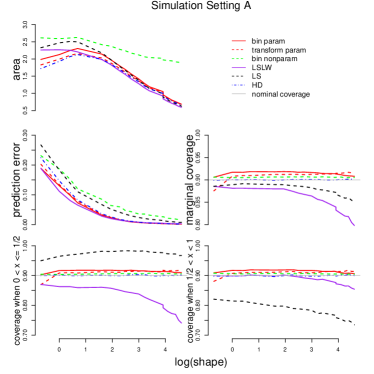
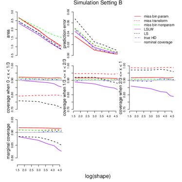
Refer to caption
Refer to caption
Figure 5: Area, prediction error, and bin-wise coverage for parametric, nonparametric, LS, LSLW conformal prediction region, and the highest density prediction region for gamma GLM regression with n=250𝑛250n=250. Simulation setting A is shown at left, and setting B at right. The average of 50 Monte Carlo samples at each shape parameter value in these simulation settings form the lines that are depicted in this figure.
Refer to caption
Refer to caption
Figure 6: Area, prediction error, and bin-wise coverage for parametric, nonparametric, LS, LSLW conformal prediction region, and the highest density prediction region for gamma GLM regression with n=500𝑛500n=500. Simulation setting A is shown at left, and setting B at right. The average of 50 Monte Carlo samples at each shape parameter value in these simulation settings form the lines that are depicted in this figure.
Refer to caption
Figure 7: Plot of the estimated coverage probabilities of prediction regions across x𝑥x and shape parameter values when the model is correctly specified, n=150𝑛150n=150, and the number of bins is equal to 222. The average of 250 Monte Carlo samples at each shape parameter value in these simulation settings form the lines that are depicted in this figure.
Refer to caption
Figure 8: Plot of the estimated coverage probabilities of prediction regions across x𝑥x and shape parameter values when the model is misspecified, n=150𝑛150n=150, and the number of bins is equal to 222. The average of 250 Monte Carlo samples at each shape parameter value in these simulation settings form the lines that are depicted in this figure.

Appendix C Plots of conformal prediction regions

C.1 Plots when Gamma model is correctly specified
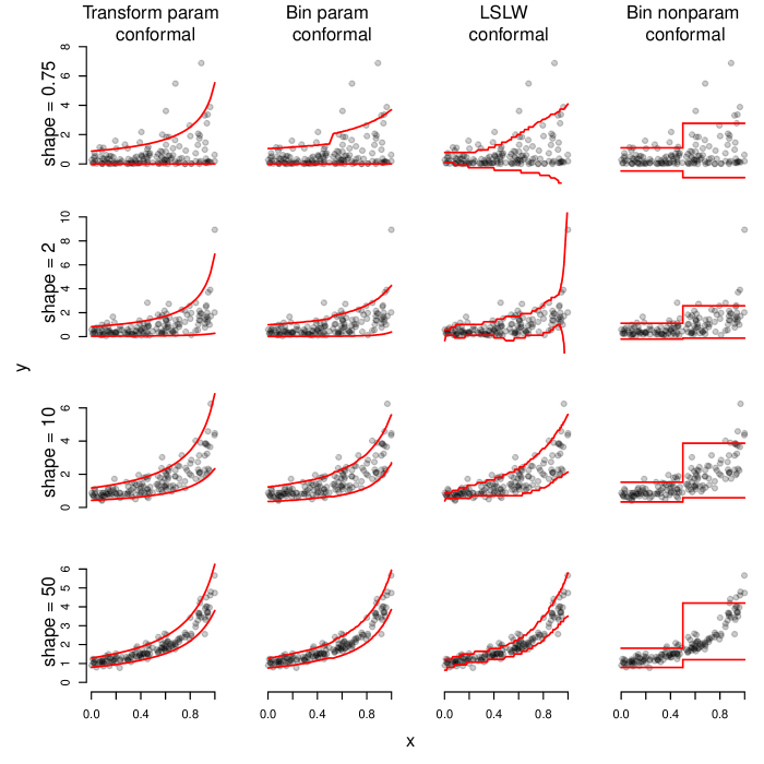
Refer to caption
Figure 9: Illustration of conformal prediction regions for Gamma regression under simulation setting A with n=150𝑛150n=150, α=0.10𝛼0.10\alpha=0.10, and the number of bins equals 2.
Refer to caption
Figure 10: Illustration of conformal prediction regions for Gamma regression under simulation setting A with n=250𝑛250n=250, α=0.10𝛼0.10\alpha=0.10, and the number of bins equals 3.
Refer to caption
Figure 11: Illustration of conformal prediction regions for Gamma regression under simulation setting A with n=500𝑛500n=500, α=0.10𝛼0.10\alpha=0.10, and the number of bins equals 3.

C.2 Plots when model is misspecified
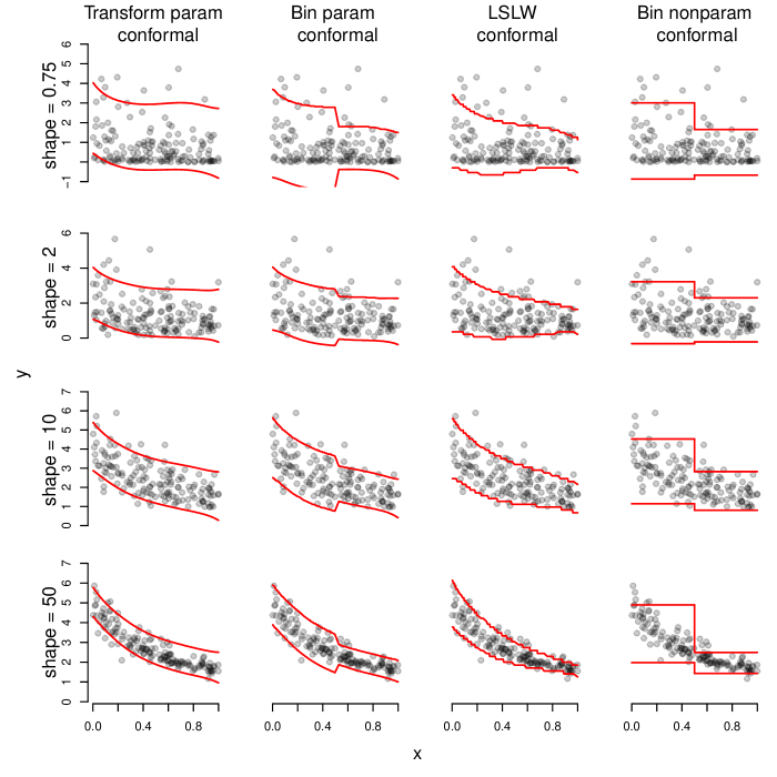
Refer to caption
Figure 12: Illustration of conformal prediction regions for Gamma regression under simulation setting B with n=150𝑛150n=150, α=0.10𝛼0.10\alpha=0.10, and the number of bins equals 2.
Refer to caption
Figure 13: Illustration of conformal prediction regions for Gamma regression under simulation setting B with n=250𝑛250n=250, α=0.10𝛼0.10\alpha=0.10, and the number of bins equals 3.
Refer to caption
Figure 14: Illustration of conformal prediction regions for Gamma regression under simulation setting B with n=500𝑛500n=500, α=0.10𝛼0.10\alpha=0.10, and the number of bins equals 3.

C.3 Plots when linear regression model is correctly specified
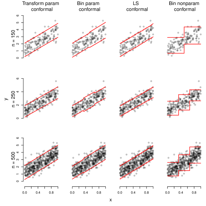
Refer to caption
Figure 15: Illustration of conformal prediction regions for linear regression under simulation setting C with α=0.10𝛼0.10\alpha=0.10.

Appendix D Example from README file in Eck (2018)

In this section we illustrate conformal prediction regions through a gamma regression example with perfect model specification when the model is known, the model can be parameterized as in displayed equation 12 of the main text, and the model does not have additive symmetric errors. We also compare conformal prediction regions to the oracle highest density region under the correct model. This example is included in the README file of the corresponding R package Eck (2018).

In this example we set the sample size to n=500𝑛500n=500 and we consider the gamma regression model with a single predictor with inverse link function (default in glm package). The predictors were generated independently as XiU(0,1)similar-tosubscript𝑋𝑖𝑈01X_{i}\sim U(0,1), i=1𝑖1i=1, \ldots, n𝑛n. We specified that β=[0.25, 2]𝛽superscript0.252\beta=[0.25,\,2]^{\prime}. The response variable was generated using rgamma with the shape parameter ϕ=2italic-ϕ2\phi=2 and the rate as 2[1,Xi]β2superscript1subscript𝑋𝑖𝛽2[1,\,X_{i}]^{\prime}\beta. Therefore we have iid data (Xi,Yi)subscript𝑋𝑖subscript𝑌𝑖(X_{i},Y_{i}) from a continuous distribution where Yi|Xiconditionalsubscript𝑌𝑖subscript𝑋𝑖Y_{i}|X_{i} is a GLM that can be parameterized as in displayed equation 12 of the main text.
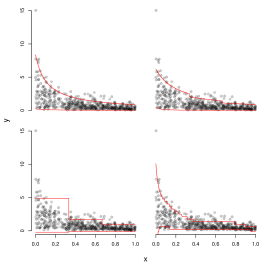
Refer to caption
Figure 16: Depiction of four prediction regions when n=500𝑛500n=500. The description of the gamma regression data generating process is outlined in the README file of the corresponding R package Eck (2018). Sim setting: shape = 222, bins = 333. The regions are depicted as follows: transformation based parametric conformal prediction (top-left panel), binned parametric conformal prediction region (top-right panel), binned nonparametric conformal prediction region (bottom-left panel), and LSLW conformal prediction region (bottom-right panel).

Figure 16 shows prediction regions for four of the five prediction regions considered. The top row depicts the transformation parametric conformal prediction region (left panel) and the binned parametric conformal prediction region (right panel). The bottom row depicts the binned nonparametric conformal prediction region (left panel) and the LSLW conformal prediction region (right panel). The bin width was specified as 1/3 for the binned conformal prediction regions. We see that the binned parametric conformal prediction region is a close discretization of the transformation conformal prediction region, the nonparametric conformal prediction region is quite jagged and unnatural, and the LSLW conformal prediction region includes negative response values and is jagged. In Figure 17 we see that the transformation based parametric conformal prediction region closely resembles the HD prediction region, and that the binned parametric conformal prediction region is a close descretization of the HD prediction region.
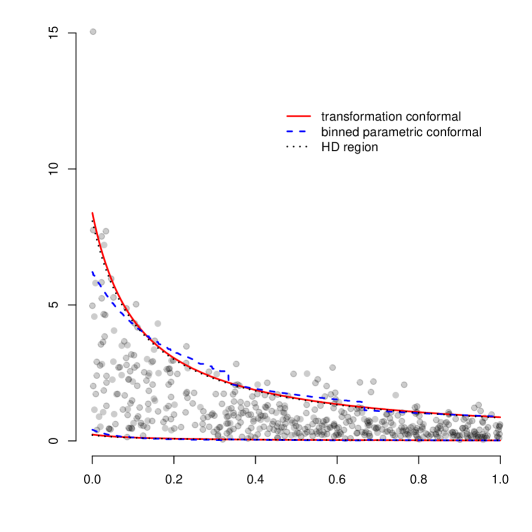
Refer to caption
Figure 17: Depiction of both parametric conformal prediction regions in Figure 16 and the HD region.

All of the presented prediction regions exhibit close to finite-sample marginal validity and local validity with respect to binning. However, the transformation conformal prediction region, LSLW conformal prediction region, and the HD prediction region do not exhibit finite-sample local validity in the second bin and the HD prediction region does not quite possess finite-sample marginal validity. The binned parametric conformal prediction region is smallest in size with an estimated area of 2.19. The HD prediction region is a close second with an estimated area of 2.21. The transformation conformal prediction region is a respectable third with an estimated area of 2.26. LSLW conformal prediction region has an estimated area of 2.56 and The nonparametric conformal prediction region has an estimated area of 2.68. Under correct model specification, the parametric conformal prediction regions are similar in performance to that of the highest density prediction region.

Performance of these prediction regions under the same model specification in this example is investigated further in a Monte Carlo simulation study. The results of this Monte Carlo simulation study are consistent with those presented here. Details are included in the reproducible technical report available at https://github.com/DEck13/conformal.glm/tree/master/techreport.

References

  • American Diabetes Association [2010] American Diabetes Association. Diagnosis and classification of diabetes mellitus. Diabetes Care, 33(Supplement 1):S62–S69, 2010.
  • Balasubramanian et al. [2014] Vineeth Balasubramanian, Shen-Shyang Ho, and Vladimir Vovk. Conformal Prediction for Reliable Machine Learning: Theory, Adaptations and Applications. Morgan Kaufmann, Boston, 2014.
  • Bobkov and Götze [1999] Sergej G Bobkov and Friedrich Götze. Exponential integrability and transportation cost related to logarithmic Sobolev inequalities. Journal of Functional Analysis, 163(1):1–28, 1999.
  • Bosc et al. [2019] Nicolas Bosc, Francis Atkinson, Eloy Felix, Anna Gaulton, Anne Hersey, and Andrew R Leach. Large scale comparison of QSAR and conformal prediction methods and their applications in drug discovery. Journal of Cheminformatics, 11(1):4, 2019.
  • Burnaev and Vovk [2014] Evgeny Burnaev and Vladimir Vovk. Efficiency of conformalized ridge regression. In Conference on Learning Theory, pages 605–622, 2014.
  • Chernozhukov et al. [2018a] Victor Chernozhukov, Kasper Wüthrich, and Yinchu Zhu. An exact and robust conformal inference method for counterfactual and synthetic controls. preprint, 2018a. URL arXiv:1712.09089.
  • Chernozhukov et al. [2018b] Victor Chernozhukov, Kasper Wüthrich, and Yinchu Zhu. Exact and robust conformal inference methods for predictive machine learning with dependent data. preprint, 2018b. URL arXiv:1802.06300.
  • Chernozhukov et al. [2019] Victor Chernozhukov, Kasper Wüthrich, and Yinchu Zhu. Distributional conformal prediction. preprint, 2019. URL arXiv:1909.07889.
  • Cho et al. [2018] NH Cho, JE Shaw, S Karuranga, Y Huang, JD da Rocha Fernandes, AW Ohlrogge, and B Malanda. IDF Diabetes Atlas: Global estimates of diabetes prevalence for 2017 and projections for 2045. Diabetes Research and Clinical Practice, 138:271–281, 2018.
  • Ciollaro et al. [2018] Mattia Ciollaro, Jessi Cisewski, Peter E. Freeman, Christopher R. Genovese, Jing Lei, Ross O’Connell, and Larry Wasserman. Functional regression for quasar spectra. preprint, 2018. URL arXiv:1404.3168.
  • Cortés-Ciriano and Bender [2018] Isidro Cortés-Ciriano and Andreas Bender. Deep confidence: A computationally efficient framework for calculating reliable prediction errors for deep neural networks. Journal of Chemical Information and Modeling, 2018.
  • Cortés-Ciriano and Bender [2019] Isidro Cortés-Ciriano and Andreas Bender. Concepts and applications of conformal prediction in computational drug discovery. arXiv:1908.03569, 2019.
  • Csörgő and Révész [1978] Miklós Csörgő and Pál Révész. Strong approximations of the quantile process. The Annals of Statistics, pages 882–894, 1978.
  • Devetyarov et al. [2012] Dmitry Devetyarov, Ilia Nouretdinov, Brian Burford, Stephane Camuzeaux, Aleksandra Gentry-Maharaj, Ali Tiss, Celia Smith, Zhiyuan Luo, Alexey Chervonenkis, Rachel Hallett, Volodya Vovk, Mike Waterfield, Rainer Cramer, John F. Timms, John Sinclair, Usha Menon, Ian Jacobs, and Alex Gammerman. Conformal predictors in early diagnostics of ovarian and breast cancers. Progress in Artificial Intelligence, 1(3):245–257, 2012.
  • Djellout et al. [2004] Hacene Djellout, Arnaud Guillin, and Liming Wu. Transportation cost-information inequalities and applications to random dynamical systems and diffusions. The Annals of Probability, 32(3B):2702–2732, 2004.
  • Dunn and Wasserman [2018] Robin Dunn and Larry Wasserman. Distribution-free prediction sets with random effects. preprint, 2018. URL arXiv:1809.07441.
  • Eck [2018] Daniel J. Eck. conformal.glm: Conformal Prediction for Generalized Linear Regression Models, 2018. https://github.com/DEck13/conformal.glm.
  • Eklund et al. [2015] Martin Eklund, Ulf Norinder, Scott Boyer, and Lars Carlsson. The application of conformal prediction to the drug discovery process. Annals of Mathematics and Artificial Intelligence, 74(1-2):117–132, 2015.
  • Faraway [2016] Julian Faraway. faraway: Functions and Datasets for Books by Julian Faraway, 2016. https://cran.r-project.org/web/packages/faraway/index.html.
  • Ferguson [1996] Thomas S. Ferguson. A course in large sample theory, 1996.
  • Gammerman and Vovk [2007] Alexander Gammerman and Vladimir Vovk. Hedging Predictions in Machine Learning: The Second Computer Journal Lecture . The Computer Journal, 50(2):151–163, 02 2007.
  • Heikes et al. [2008] Kenneth E Heikes, David M Eddy, Bhakti Arondekar, and Leonard Schlessinger. Diabetes risk calculator: a simple tool for detecting undiagnosed diabetes and pre-diabetes. Diabetes care, 31(5):1040–1045, 2008.
  • Izbicki et al. [2019] Rafael Izbicki, Gilson Y. Shimizu, and Rafael B. Stern. Distribution-free conditional predictive bands using density estimators. preprint, 2019. URL arXiv:1910.05575.
  • Ji et al. [2018] Changge Ji, Fredrik Svensson, Azedine Zoufir, Andreas Bender, and Alfonso Valencia. eMolTox: prediction of molecular toxicity with confidence. Bioinformatics, 1:2, 2018.
  • Johansson et al. [2018] Ulf Johansson, Henrik Linusson, Tuve Löfström, and Henrik Boström. Interpretable regression trees using conformal prediction. Expert Systems With Applications, 97:394–404, 2018.
  • Komlós et al. [1975] János Komlós, Péter Major, and Gábor Tusnády. An approximation of partial sums of independent rv’-s, and the sample df. i. Zeitschrift für Wahrscheinlichkeitstheorie und verwandte Gebiete, 32(1-2):111–131, 1975.
  • Lambrou et al. [2009] Antonis Lambrou, Harris Papadopoulos, and Alex Gammerman. Evolutionary conformal prediction for breast cancer diagnosis. Proceedings of 9th International Conference on Information Technology and Applications in Biomedicine, pages 1–4, 2009.
  • Ledoux [1999] Michel Ledoux. Concentration of measure and logarithmic sobolev inequalities. Lecture Notes in Math, 1709:120–216, 1999.
  • Ledoux [2001] Michel Ledoux. The Concentration of Measure Phenomenon. American Mathematical Society, 2001.
  • Lei and Wasserman [2014] Jing Lei and Larry Wasserman. Distribution-free prediction bands for nonparametric regression. Journal of the Royal Statistical Society series B, 76, 1:71–96, 2014.
  • Lei et al. [2013] Jing Lei, James Robins, and Larry Wasserman. Distribution-free prediction sets. Journal of the American Statistical Association, 108:278–287, 2013.
  • Lei et al. [2015] Jing Lei, Alessandro Rinaldo, and Larry Wasserman. A conformal prediction approach to explore functional data. Annals of Mathematics and Artificial Intelligence, 74:29–43, 2015.
  • Lei et al. [2018] Jing Lei, Max G’Sell, Alessandro Rinaldo, Ryan J Tibshirani, and Larry Wasserman. Distribution-free predictive inference for regression. Journal of the American Statistical Association, 113(523):1094–1111, 2018.
  • McCullagh and Nelder [1989] Peter McCullagh and John A Nelder. Generalized Linear Models. CRC press, 1989.
  • Meredith and Kruschke [2018] Mike Meredith and John Kruschke. HDInterval: Highest (Posterior) Density Intervals, 2018. https://cran.r-project.org/web/packages/HDInterval/.
  • Miao [2010] Yu Miao. Concentration inequality of maximum likelihood estimator. Applied Mathematics Letters, 23(10):1305–1309, 2010.
  • Norinder et al. [2018a] Ulf Norinder, Ernst Ahlberg, and Lars Carlsson. Predicting Ames mutagenicity using conformal prediction in the Ames/QSAR International Challenge Project. Mutagenesis, 2018a.
  • Norinder et al. [2018b] Ulf Norinder, Glenn Myatt, and Ernst Ahlberg. Predicting aromatic amine mutagenicity with confidence: A case study using conformal prediction. Biomolecules, 8(3):85, 2018b.
  • Papadopoulos et al. [2011] Harris Papadopoulos, Vladimir Vovk, and Alex Gammerman. Inductive conformal prediction: Theory and application to neural networks. Journal of Artificial Intelligence Research, 40:815–840, 2011.
  • R Core Team [2019] R Core Team. R: A Language and Environment for Statistical Computing. R Foundation for Statistical Computing, Vienna, Austria, 2019. https://www.R-project.org/.
  • Romano et al. [2019a] Yaniv Romano, Rina F. Barber, Chiara Sabatti, and Emmanuel J. Candés. With malice towards none: Assessing uncertainty via equalized coverage. preprint, 2019a. URL arXiv:1908.05428.
  • Romano et al. [2019b] Yaniv Romano, Evan Patterson, and Emmanuel J. Candés. Conformalized quantile regression. preprint, 2019b. URL arXiv:1905.03222.
  • Sesia and Candés [2019] Matteo Sesia and Emmanuel J. Candés. A comparison of some conformal quantile regression methods. preprint, 2019. URL arXiv:1909.05433.
  • Shafer and Vovk [2008] Glenn Shafer and Vladimir Vovk. A tutorial on conformal prediction. Journal of Machine Learning Research, 9:371–421, 2008.
  • Svensson et al. [2018a] Fredrik Svensson, Avid M Afzal, Ulf Norinder, and Andreas Bender. Maximizing gain in high-throughput screening using conformal prediction. Journal of Cheminformatics, 10(1):7, 2018a.
  • Svensson et al. [2018b] Fredrik Svensson, Natalia Aniceto, Ulf Norinder, Isidro Cortes-Ciriano, Ola Spjuth, Lars Carlsson, and Andreas Bender. Conformal regression for quantitative structure–activity relationship modeling–quantifying prediction uncertainty. Journal of Chemical Information and Modeling, 58(5):1132–1140, 2018b.
  • Tibshirani [2016] Ryan Tibshirani. conformalInference: Tools for conformal inference in regression, 2016. https://github.com/ryantibs/conformal.
  • Toccaceli et al. [2017] Paolo Toccaceli, Ilia Nouretdinov, and Alexander Gammerman. Conformal prediction of biological activity of chemical compounds. Annals of Mathematics and Artificial Intelligence, 81(1-2):105–123, 2017.
  • Trench [2013] William F. Trench. Introduction to Real Analysis. 2013. Relevant material from Supplement 1.
  • Villani [2008] Cédric Villani. Optimal Transport: Old and New, volume 338. Springer Science & Business Media, 2008.
  • Vovk [2012] Vladimir Vovk. Conditional validity of inductive conformal predictors. Proceedings of Machine Learning Research, 25:475–490, 2012.
  • Vovk et al. [2005] Vladimir Vovk, Alex Gammerman, and Glenn Shafer. Algorithmic Learning in a Random World. Springer, 2005.
  • Wainwright [2019] Martin J. Wainwright. High-Dimensional Statistics: A Non-Asymptotic Viewpoint. Cambridge Series in Statistical and Probabilistic Mathematics, 2019. URL https://www.stat.berkeley.edu/~mjwain/stat210b/Chap2_TailBounds_Jan22_2015.pdf.
  • Wang et al. [2018] Di Wang, Ping Wang, and Junzhi Shi. A fast and efficient conformal regressor with regularized extreme learning machine. Neurocomputing, 304:1–11, 2018.
  • Willems et al. [1997] James P Willems, J Terry Saunders, Dawn E Hunt, and John B Schorling. Prevalence of coronary heart disease risk factors among rural blacks: a community-based study. Southern Medical Journal, 90(8):814–820, 1997.
  • World Health Organization [2011] World Health Organization. Use of glycated haemoglobin (HbA1c) in diagnosis of diabetes mellitus: abbreviated report of a WHO consultation. Technical report, Geneva: World Health Organization, 2011.