Thermal Fracture Kinetics of Heterogeneous Semiflexible Polymers

Abstract

The fracture and severing of polymer chains plays a critical role in the failure of fibrous materials and the regulated turnover of intracellular filaments. Using continuum wormlike chain models, we investigate the fracture of semiflexible polymers via thermal bending fluctuations, focusing on the role of filament flexibility and dynamics. Our results highlight a previously unappreciated consequence of mechanical heterogeneity in the filament, which enhances the rate of thermal fragmentation particularly in cases where constraints hinder the movement of the chain ends. Although generally applicable to semiflexible chains with regions of different bending stiffness, the model is motivated by a specific biophysical system: the enhanced severing of actin filaments at the boundary between stiff bare regions and mechanically softened regions that are coated with cofilin regulatory proteins. The results presented here point to a potential mechanism for disassembly of polymeric materials in general and cytoskeletal actin networks in particular by the introduction of locally softened chain regions, as occurs with cofilin binding.

1 Introduction

The fracture properties of polymeric solids pose a key constraint on the manufacture and design of a vast array of man-made materials for load-bearing or weather-resistant purposeskausch1987polymer ; ward2012mechanical . Furthermore, polymeric materials serve as some of the most important structural and information-bearing components in living organisms, and their rupture (whether through mechanical or environmental stress or through regulated turnover) has a crucial role to play in biological processes ranging from cell divisionzhou2015mechanical , to tumorigenesisvan2001chromosomal , to cell motilitypollard2003cellular . Theoretical and experimental explorations of failure mechanisms have established that the fracture of polymeric solids relies in large part on the scission of individual polymer filaments, with the dynamics and stress-dependence of fracture governed by the kinetics of molecular ruptureregel1972kinetic ; tomashevskii1975kinetic ; kausch1987polymer . At the molecular scale, fracture is inherently a thermal process, where the activation energy is lowered by the application of stress on individual bonds along the filamenttomashevskii1975kinetic .

Fragmentation of a polymer filament is accelerated when externally applied stresses become locally concentrated in specific regions. This principle underlies, for instance, the fragmentation of DNA at discrete folding points under extensional flowreese1990fracture , the rupture of microtubules through buckling during spindle reorganizationschiel2011endocytic and traumatic axonal injurytang2010mechanical , and the severing of actin bundles by myosin-driven compression in motile cellsmedeiros2006myosin ; tsai2019efficient . Local discontinuities in mechanical properties tend to concentrate externally applied stress, leading to preferential fracture of materials at these discontinuous regionssuresh2001graded ; cruz2015mechanical .

In the case of thermally driven fracture, the effect of mechanical inhomogeneities in a filament is poorly understood. Prior theoretical work showed that thermal energy is equally partitioned among spatial degrees of freedom in general equilibrium one-dimensional systemsbar2015spatial . However, fracture is inherently a transient, kinetic process. Understanding fracture rates requires moving beyond equilibrium distributions to consider the dynamics of thermal fluctuations in a polymer filament. Here we focus on the role of spatial heterogeneity of mechanical properties in accelerating thermally induced fracture of semiflexible chains.

The general problem of fracture rates in a thermalized, mechanically heterogeneous, polymer filament is motivated in part by a biological system: the cofilin-mediated severing of cytoskeletal actin filaments. Actin is a semiflexible polymer that forms bundles and networks responsible for maintaining cell-scale mechanical properties as well as driving processes such as lamellipodial motility, cytokinesis, and embryonic patterningfletcher2010cell ; salbreux2012actin . Much of the biological behavior of actin networks relies on the dynamic turnover of individual actin filaments, which is accelerated by the actin-binding protein cofilin. Cofilin assembles cooperatively along actin chains, locally decreasing their bending stiffness and resulting in mechanically heterogeneous partially decorated filamentsmcgough1999ADF ; mccullough2008cofilin ; pfaendtner2010actin ; mccullough2011cofilin ; fan2013molecular . Such filaments fragment, without additional energy input, preferentially at the boundary of cofilinated segmentscruz2009cofilin ; mccullough2011cofilin ; elam2013biophysics . While missing bonds at these discontinuities may account for their increased fragility, particularly under stressschramm2017actin , an additional contribution to enhanced severing has been proposed that relies on the concentration of stress at the discontinuities between cofilinated and bare actin segmentscruz2015mechanical ; schramm2017actin . Here, we explore the physical plausibility of enhanced fracture at a junction between soft and stiff regions, in a purely thermal system (ie: in the absence of externally applied compressive forces).

2 Mechanical model for heterogeneous filament

We consider the thermally driven fracture of a mechanically heterogeneous filament, by building upon the well-established continuum “worm-like chain” (WLC) model for semiflexible polymerskratky1949wlc ; spakowitz2005end . Prior work on the statistical mechanics of heterogeneous and kinked worm-like chains has established a framework for analytically calculating their distribution functionswiggins2005exact ; zhang2010intrinsic ; koslover2013systematic . Here we focus on the simplest heterogeneous chain: a diblock copolymer consisting of two WLC of equal length $L$ and bending persistence lengths $\ell_{p,1}\geq\ell_{p,2}$. The chains are grafted together at a point junction (Fig. 1a), whose bending energy is defined as

$$\begin{split}\frac{1}{k_{b}T}E_{\text{junc}}&=\kappa(1-\rho),\\ \rho&=\cos\theta,\end{split}$$ (1)

where $k_{b}T$ is the thermal energy and $\theta$ is the bending angle between chain tangents at the junction. The junction represents a short portion of the chain of length $\Delta$, with $\Delta\ll L$. In our model, this junction is treated as a single point with stiffness $\kappa=\ell_{p,1}/\Delta$. In particular, we note that this junction represents the behavior of the last short segment of stiff chain just before the attachment of the softer chain.

The mechanics of the heterogeneous chain are fully defined by three dimensionless parameters: chain half-length $N=L/(2\ell_{p,1})$, junction length $\hat{\Delta}=\Delta/L=1/(2\kappa N)$, and heterogeneity $h=\ell_{p,1}/\ell_{p,2}$.

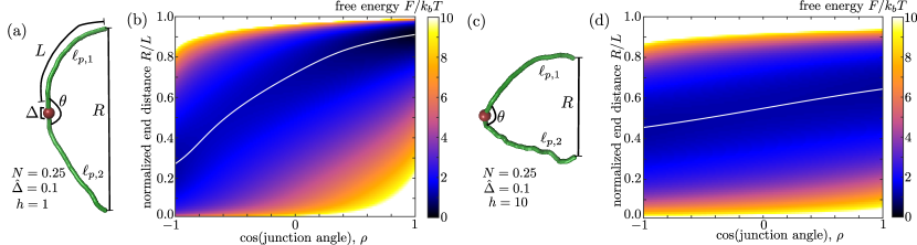
Figure 1: Model schematic and energy landscapes. (a) Sample configuration of homogeneous chain, with model parameters labeled. (b) Free energy landscape for homogeneous chain shown in (a), plotted as a function of junction bending and normalized end distance. White line markes the lowest energy path to steeper junction angles. (c-d) Sample configuration and corresponding free energy landscape for heterogeneous chain with $\ell_{p,1}/\ell_{p,2}=10$.

The overall partition function [$G_{\text{tot}}(\vec{R},\rho)$] for this model is computed from prior results derived for worm-like chains with end constraintsspakowitz2005end ; mehraeen2008end ; koslover2013systematic . We start with the partition function [$\hat{G}(\vec{R},\vec{u};L,\ell_{p})$] for a WLC chain or length $L$, persistence length $\ell_{p}$, with one end at the origin, the other end at position $\vec{R}$, and final end tangent $\vec{u}$. After a Fourier transform from $\vec{R}$ to $\vec{k}$, this function is given by:

$$\begin{split}\widehat{G}(\vec{k},\vec{u};L,\ell_{p})=\frac{1}{4\pi}\sum_{l=0}^{\infty}\mathcal{G}_{0,l}\left(2\ell_{p}k,\frac{L}{2\ell_{p}}\right)P_{l}(\vec{u}\cdot\vec{k}),\end{split}$$ (2)

where $P_{l}$ are Legendre polynomials and the $\mathcal{G}^{m}_{l_{0},l_{f}}$ coefficients refer to previously defined continued fraction termsspakowitz2005end . For a heterogeneous wormlike chain with end-to-end vector $\vec{R}$ and junction angle $\theta$, the partition function is obtained from the convolution of two such propagators

$$\begin{split}G_{\text{tot}}(\vec{R},\rho;L,\ell_{p,1},\ell_{p,2})=&\int d\vec{R}_{j}d\vec{u}_{j}d\phi\hat{G}(\vec{R_{j}},\vec{u_{j}};L,\ell_{p,1})\\ \times&\hat{G}(\vec{R}-\vec{R_{j}},\vec{\mathbf{\Omega}(\theta,\phi)\cdot u_{j}};L,\ell_{p,2})\\ \end{split}$$ (3)

where $\vec{R}_{j}$ is junction position, $\vec{u}_{j}$ is the incoming tangent to the junction, and $\Omega(\phi,\theta)$ is a rotation matrix that rotates the cannonical coordinate system by Euler angles $(\phi,\theta,0)$. The Fourier transform in space, together with an application of the spherical harmonic addition theoremarfken2005mathematical , allows this convolution to be simplified to:

$$\begin{split}\widehat{G}_{\text{tot}}(\vec{k},\rho;N,1,h)=\frac{1}{2}\sum_{\ell=0}^{\infty}P_{l}(\rho)\mathcal{G}_{0,l}\left(k,N\right)\mathcal{G}_{0,l}\left(\frac{k}{h},hN\right),\end{split}$$ (4)

where we have nondimensionalized all length units by $2\ell_{p,1}$. Finally, the Fourier inversion is computed according tomehraeen2008end

$$\begin{split}G_{\text{tot}}(\vec{R},\rho)=\frac{1}{(2\pi^{2})(2\ell_{p,1})^{3}}\int_{0}^{\infty}\!\!dk\,\frac{k\sin(2kNr)}{2Nr}\,\widehat{G}_{\text{tot}}(k,\rho),\end{split}$$ (5)

where $r=|R|/(2L)$ is the normalized end separation of the joint chain. This propagator is normalized such that $\int d\vec{R}G_{\text{tot}}(\vec{R},\rho)=1$ for each value of $\rho$.

The free energy ($F$) of the chain is then defined as the log of the partition function, with an additional term for the bending of the junction angle. Namely,

$$\begin{split}\frac{1}{k_{b}T}F(r,\rho)=\kappa(1-\rho)-\log\left[r^{2}G_{\text{tot}}(r,\rho)\right]\end{split}$$ (6)

This free energy landscape is plotted in Fig. 1 for a homogeneous, stiff chain and a heterogeneous chain.

We focus on filament fracture at the junction point, assuming that fracture will occur when thermal fluctuations push the junction energy ($E_{\text{junc}}$) above some predefined cutoff ($E^{*}$). This model represents a fracture process where the junction must hop over a transition energy barrier, with the cosine of the bending angle $\rho$ as the reaction coordinate. Chains with a more flexible junction (lower $\kappa$) will have to reach more extreme junction bending ($\rho^{*}=1-E^{*}/\kappa$) than chains with a more stiff junction (higher $\kappa$). This model is consistent with previous analyses of experimental data on fracture of short cofilin-decorated actin filaments that points to fracture occuring beyond a critical bending angle that increases with lower filament persistence lengthmccullough2011cofilin . Critical energies of approximately $22$kT have been estimated for the severing of bare actin filamentsmccullough2011cofilin .

The overall rate of fracture is obtained from the mean first passage time (MFPT) to the critical value $\rho^{*}$, as the system fluctuates thermally over the free energy landscape plotted in Fig. 1. The kinetics of fracture are thus determined by a free energy barrier incorporating both the junction bending energy and the configurational free energy of the worm-like chains. For a homogeneously stiff chain, surmounting this barrier along the minimum energy path requires bringing the ends of the chain closer together (Fig. 1c). For the heterogeneous chain, by contrast, the cutoff junction angle can be reached without substantial change in the end-to-end distance (Fig. 1d). The importance of this effect in determining the overall time to fracture depends on the dynamics of the end-to-end coordinate $r$ compared to the dynamics of the junction angle.

3 Dynamics over Free Energy Landscape

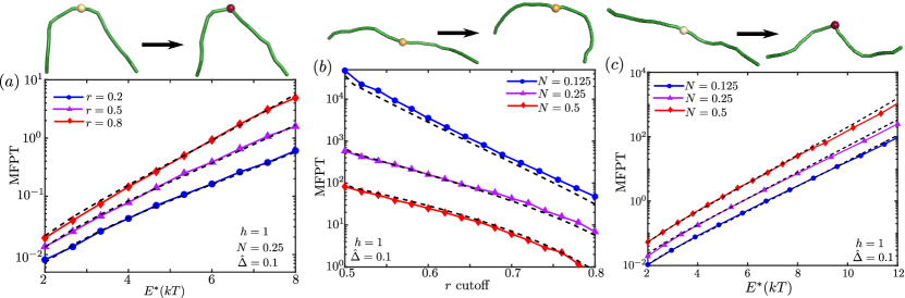
Figure 2: Comparison of approximate dynamics over free energy landscapes versus Brownian dynamics simulations. (a) MFPT to a cutoff junction energy $E^{*}$, for fixed end distance. (b) MFPT to a cutoff value of the normalized end-to-end distance $r$. (c) MFPT to a junction energy $E^{*}$, with free chain ends. In all cases, dashed black lines correspond to first passage times calculated from the free energy landscapes, solid lines correspond to Brownian dynamics simulations. All times are non-dimensionalized by $D^{(0)}_{\rho}$.Top panels show example start and end configurations, with junction color indicating energy at the junction.

To calculate kinetics over the free energy landscape, we make the simplifying assumption that for each value of the end distance $r$, the kinetics of transition to the cutoff $\rho^{*}$ can be described by a single time-scale — the mean first passage time $\tau(\rho^{*};r)$ along a horizontal slice of the landscape. Dynamics along the angular coordinate are defined by a variable friction coefficient that depends on the value of the junction angle,

$$\begin{split}\zeta(\rho)=\frac{k_{B}T}{D^{(0)}_{\rho}}\frac{5-3\rho}{6(1-\rho^{2})}\end{split}$$ (7)

where $D^{(0)}_{\rho}=\frac{k_{B}T}{\mu\Delta^{3}}$ and $\mu$ is the translational friction coefficient per unit length of the chain. This expression is derived from the dynamics of two connected rigid links (Appendix A). We note that the numerical prefactor in the friction coefficient (Eq. 7) depends on mapping from the behavior of two rigid links to the dynamics of a point-like kink representing a short length of semiflexible chain. This prefactor is not directly determined by our theory, and we fit the appropriate length of links to establish this mapping (specifically, $\ell_{\text{link}}=2\Delta$) by matching the theory to Brownian dynamics simulations of semiflexible chains, as described below. This is the only fitting parameter in the model, a single value (as shown in Eq. 7) is used for all results described.

The mean first passage time over a one-dimensional landscape can be computed from the Fokker-Planck equationfox1986functional ; risken1996fokker ; koslover2009twist , appropriately modified for spatially varying diffusivitylau2007state (Appendix B). Specifically, the fracture time for a fixed value of $r$ is given by

$$\begin{split}&\tau(\rho^{*},r)=\frac{1}{\int_{\rho^{*}}^{1}e^{-F(r,\rho)/k_{b}T}d\rho}\times\\ &\times\left[\int_{\rho^{*}}^{1}d\rho\int_{\rho^{*}}^{\rho}d\rho^{\prime}\int_{\rho^{\prime}}^{1}d\rho^{\prime\prime}\frac{\zeta(\rho^{\prime})}{k_{b}T}e^{\left(F(r,\rho^{\prime})-F(r,\rho^{\prime\prime})-F(\rho)\right)/k_{b}T}\right].\end{split}$$ (8)

Brownian dynamics simulations of a discretized WLC model are used to validate our calculations of the mean first passage time for fixed values of the end distance, with the free energy landscape given by Eq. 6 and the friction coefficient in Eq. 7. As shown in Fig. 2a, the continuum chain theory accurately reproduces the kinetics of reaching a high junction angle in simulations.

The overall mean first passage time to fracture can be computed by considering a system that fluctuates over discrete states in the normalized end distance, with state $i$ corresponding to $r_{i}=i\delta r$, and the discretization set to $\delta r=0.01$. The system is assumed to start in thermal equilibrium, with the probability of starting in state $i$ set by a Boltzmann factor corresponding to the free energy of that state: $F_{i}=-k_{B}T\log\int d\rho\exp[-F(r_{i},\rho)/k_{B}T]$. Transitions between states occur with rate constants $k_{i}^{(\pm)}$, given by

$$\begin{split}k_{i}^{(\pm)}&=\frac{\frac{k_{R}}{\delta r^{2}}(F_{i\pm 1}-F_{i})}{\exp(F_{i\pm 1}-F_{i})-1},\\ \end{split}$$ (9)

as derived from a discretization of the Fokker-Planck equationwang2003robust . The dynamic prefactor is taken to be the time-scale for three-dimensional translational diffusion of a chain of length $L$ over a length scale $\Delta R=2L\delta r$, according to:

$$\begin{split}\frac{k_{R}}{\delta r^{2}}&=\frac{6k_{B}T}{(\mu L)(2L\delta r)^{2}}.\end{split}$$ (10)

This approximate model for dynamics in the end-to-end distance gives comparable results to Brownian dynamics simulations that sample the average time required to reach a cutoff end-to-end distance for chains starting in thermal equilibrium (Fig. 2b). These simulations are compared against an analytical model for dynamics over a discrete one-dimensional landscapekoslover2012force , with the transition rates given by Eq. 9, 10.

To put together both dimensions of the energy landscape, we treat fracture as a Poissonian process within each particular end-distance state, with average time given by $\tau_{i}=\tau(\rho^{*},r_{i})$. We compute the overall mean time to fracture for a system that fluctuates over these states using a matrix inversion method, as described in previous work on the kinetics of systems with fluctuating rateskoslover2012force . This approach for representing the dynamics of the system as movement over a two-dimensional free energy landscape is validated by comparison to Brownian dynamics simulations with unconstrained homogeneous chains (Appendix C; Supplemental Videos 1, 2). As shown in Fig. 2c, Our model of dynamic fluctuations over a two-dimensional energy landscape thus appears to accurately represent the behavior of simulated chains, with respect to the time required for a junction region to hit a cutoff angle.

4 Fracture rates for heterogeneous chains

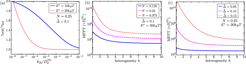
Figure 3: Chain heterogeneity enhances junction fracture rates when chain end dynamics are slow. (a) Ratio of MFPT to fracture for uniformly stiff ($h=1$) and heterogeneous ($h=10$) chains is plotted versus the relative rate of chain end dynamics compared to junction dynamics. (b-c) Time to fragmentation in the limit of infinitely slow chain end dynamics. Dimensionless MFPT is shown as a function of heterogeneity $h$ for (b) chains with a fixed junction length $\widehat{\Delta}=0.1$ and varying stiffness and (c) chains with a fixed stiffness ($N=0.25$) but varying junction length. Chains are assumed to start from an equilibrium distribution.

The overall time to fracture is dependent on the relative rate of motion in the end-to-end distance as compared to the rate of junction fluctuations (Fig. 3a). For the case of very rapid end equilibration (high $k_{R}/D_{\rho}^{(0)}$), the chain would be expected to sample all end positions over a time-scale that is short compared to the fracture time. In this limit, the fracture dynamics are determined entirely by the stiffness and friction coefficient for the junction bending ($\rho$) and are independent of the mechanical properties of the rest of the chain.

The opposite regime holds when the dynamics of the end distance are much slower than those of the junction angle. In this case, the end distance remains constant at its starting value, and the mean time to fracture is the weighted average of the individual $\tau_{i}$. Softer mechanics in one half of the chain make it more probable that a lower value of $r$ will initially be selected from the equilibrium distribution. This lower $r$ persists over time and allows the junction to more rapidly reach the cutoff angle.

Fig. 3b,c show the mean time to fracture for chains with different degrees of heterogeneity $h$ in the case of fixed end-to-end distance (infinitely slow $r$ dynamics). In this limit, a purely stiff chain will be slow to reach fracture at the junction because a higher overall chain deformation energy is required to bend the junction to the point of fracture. A purely soft chain will also be slow to reach fracture because the requisite junction angle $\theta^{*}$ to achieve the same cutoff energy will be correspondingly largermccullough2011cofilin . Rapid fracture can be achieved by a heterogeneous chain, where the junction stiffness and hence the cutoff angle are set by the stiff side of the chain, while the low persistence length of the soft side enables the junction to reach that cutoff angle without moving the chain ends or incurring a substantial cost in chain deformation energy. The enhancement due to chain heterogeneity can reach several orders of magnitude in cases where the junction must reach very steep bending angles in order to fracture (high $N$ and $\widehat{\Delta}$).

In the case where chain ends are unconstrained, calculating the fracture rate requires an estimation of the rate of chain end dynamics compared to the dynamics in the junction coordinate. The dimensionless parameter describing these relative rates is $k_{R}/D_{\rho}^{(0)}=\frac{3}{2}\widehat{\Delta}^{3}$.

For chain heterogeneity to enhance thermal fracture, this ratio of rates must be small (ie: the sampling of junction angles must be substantially faster than the end-to-end motion). However, when $\Delta$ becomes small for a chain of constant length, the junction stiffness $\kappa$ must increase and the fracture process becomes dominated by junction energetics rather than deformation of larger portions of the chain. In this limit the fracture rate becomes similar for heterogeneous and homogeneously stiff chains (Fig. 3c, 4a). If the end-to-end dynamics are slowed down by increasing the chain length $L$ while keeping the junction length $\Delta$ constant (Fig. 4b), then the stiff side of the chain becomes more flexible and the fracture enhancement from chain heterogeneity decreases. Overall, the enhancement in fracture rates for a heterogeneous chain with free end conditions maxes out at approximately $15\%$, for a heterogeneity $h=\ell_{p,1}/\ell_{p,2}=10$ (Fig. 4).

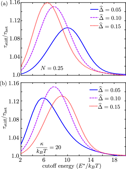
Figure 4: Enhacement in fracture rate for a heterogeneous vs homogeneous chain with free chain ends. The ratio of MFPT to fracture for a fully stiff chain ($h=1$) vs a heterogeneous chain ($h=10$) is plotted as a function of the cutoff energy. (a) Filaments with constant length $N$ but varying junction size and stiffness (solid: $\kappa=40$, dashed: $\kappa=20$, dotted: $\kappa=13$. (b) Filaments with varying length but constant junction stiffness $\kappa$ (solid: $N=0.125$, dashed: $N=0.25$, dotted: $N=0.5$).

5 Concluding Remarks

Our calculations show that filament heterogeneity can substantially enhance the rate of thermal fracture in the case of restricted end-to-end dynamics of the filament. A modest enhancement is expected for the case of a chain with freely moving ends. We note that the model developed here differs from previous athermal models for fracturecruz2015mechanical ; schramm2017actin which indicated that a heterogeneous chain concentrates stresses at the junction when the chain is forced into a buckled configuration. The enhancement in thermally driven fracture occurs despite the fact that the initial configuration of the chain is allowed to sample from the equilibrium distribution. The contrast between the case of rapid and slow $r$ equilibration (Fig. 3a) highlights the purely dynamic nature of this effect. Fracture enhancement arises from the separation in timescales between fluctuations at the junction versus moving the ends of the entire polymer. The presence of a softer chain region allows a junction to reach steep bending angles without requiring large movements of the chain ends and without paying a large energetic cost for the chain deformation.

While our model focuses on fracture in a specific junction region, at the internal end of the stiff chain segment, it provides insight into the behavior of other regions in a heterogeneous chain. In particular, regions on the soft side of the chain will behave similarly to the center of a homogeneously soft chain, and are expected to be slow to fracture because of the steep bending angle required to reach the cutoff energy. By contrast, regions located in the middle of the stiff side would require moving large segments of stiff chain to assume the requisite bending angle, again leading to slow fracture dynamics. Rapid dynamics become possible specifically close to the junction between the soft and stiff regions, but where the junction itself is still stiff.

The model with restricted chain ends is particularly relevant for the cofilin-mediated severing of actin filaments within a cytoskeletal network. In such networks cross-links and entanglements can effectively restrict the movement of certain positions along the chain, while allowing rapid equilibration of chain positions between the cross-link points. Our results indicate that in such situations introducing mechanical heterogeneity into the actin filaments by cofilin binding should substantially enhance thermal severing rates.

It should be noted that, in addition to changing the flexibility of actin filaments, cofilin binding also alters the filament twist density. Recent experiments have shown that constraining filaments to prevent torsional equilibration enhances actin filament severing by cofilin pavlov2007actin ; wioland2019torsional ; elam2013biophysics . The effect described here centers on severing due to bending fluctuations and may provide a parallel, unrelated mechanism for cofilin-driven fracture. Both twist-based and bending-based severing are expected to depend on the density and mechanics of cross-links in an actin network. By providing a feedback mechanism between network structure and actin severing dynamics, these physical effects may play an important role in regulating the self-assembly, turnover, and mechanoresponse of cytoskeletal structures.

In addition to helping unravel the mechanisms of actin severing by cofilin, the results presented here are generally applicable to the fracture of any semiflexible thermally fluctuating polymer. Enhanced rates of thermally-activated fracture in mechanically heterogeneous chains point towards general principles for controlling the stability of nanoscale systems, including polymer networks, nanotubules, and molecular threads, for a broad range of biological and industrial applications.

APPENDIX

A Angular dynamics for coupled rigid links

In this section we derive the angular dynamics for two connected rigid links, each of length $\ell$, in a highly viscous fluid. We assume each of the links has a friction coefficient per unit length $\mu$, and that there is a bending modulus $\kappa$ for the junction between the links. This simplified system serves as a basis for deriving the appropriate dynamics of the junction angle for the heterogeneous worm-like chain.

We define a given configuration of the system by the center of mass positions for the two rigid rods ($\vec{r}_{1},\vec{r}_{2}$) and their normalized orientations ($\vec{u}_{1},\vec{u}_{2}$). The overall energy for this configuration is then given by,

$$\begin{split}E=\kappa(1-\vec{u}_{1}\cdot\vec{u}_{2})+\vec{\lambda}\cdot\left(\vec{r}_{1}+\frac{\ell}{2}u_{1}-\vec{r}_{2}+\frac{\ell}{2}\vec{u}_{2}\right).\end{split}$$ (S1)

Here, the first term corresponds to the bending energy of the junction between the two rods and the second term uses a Lagrange multiplier ($\vec{\lambda}$) to enforce the connectivity of the two inextensible rods at the junction.

In the freely draining approximation, and in the absence of Brownian forces, the overdamped dynamics of such a system are defined by the equations,

$$\begin{split}\zeta_{r}\vec{\omega}_{i}&=-\vec{u}_{i}\times\frac{\partial E}{\partial u_{i}}\\ \zeta_{t}\frac{d\vec{r}_{i}}{dt}&=-\frac{\partial E}{\partial\vec{r}_{i}},\end{split}$$ (S2)

where $\vec{\omega}_{i}$ gives the rotational velocity for each rod ($i=1,2$). Here, $\zeta_{r}=\mu\ell^{3}/12$ is the rotational frictional coefficient of each rod around its center of mass and $\zeta_{t}=\mu\ell$ the translational friction coefficientdoi1988theory . The Lagrange multiplier $\vec{\lambda}$ can be obtained from the constraints:

$$\begin{split}\frac{d}{dt}\left(\vec{r}_{1}+\frac{\ell}{2}u_{1}-\vec{r}_{2}+\frac{\ell}{2}\vec{u}_{2}\right)\cdot\vec{u}_{1}=0\\ \frac{d}{dt}\left(\vec{r}_{1}+\frac{\ell}{2}u_{1}-\vec{r}_{2}+\frac{\ell}{2}\vec{u}_{2}\right)\cdot\vec{u}_{2}=0.\\ \end{split}$$ (S3)

Solving these equations yields $\vec{\lambda}\cdot\vec{u}_{i}=\frac{6\kappa(1-\rho^{2})}{\ell(5-3\rho)}$, where $\rho=\vec{u}_{1}\cdot\vec{u}_{2}$. The dynamics of the angular coordinate $\rho$ are then given by,

$$\begin{split}\frac{d\rho}{dt}=\frac{48\kappa(1-\rho^{2})}{\mu\ell^{3}(5-3\rho)}.\end{split}$$ (S4)

This expression gives the effective friction coefficient for the coordinate $\rho$ according to

$$\begin{split}\frac{d\rho}{dt}&=-\frac{1}{\zeta(\rho)}\frac{\partial E_{\text{bend}}}{\partial\rho}=-\frac{\kappa}{\zeta(\rho)}\\ \zeta(\rho)&=\frac{\mu\ell^{3}(5-3\rho)}{48(1-\rho^{2})}\end{split}$$

For the angular dynamics of a junction in a continuum worm-like chain, changes in the angle require dragging along a length of chain that should scale as the junction size $\Delta$. We select an effective link length $\ell=2\Delta$ for use in Eq. 7. The prefactor of $2$ is obtained from fitting to Brownian dynamics simulations with fixed end-to-end distance (as shown in Fig. 2a). This is the only fitting parameter in the theory and is used for all results shown in subsequent figures.

B Mean first passage time on a 1D landscape

For one-dimensional systems with spatially varying diffusivity $D(x)$ and free energy landscape $F(x)$, it has been shown that the Fokker-Planck equation which correctly reproduces the Boltzman distribution in the steady statelau2007state is given by,

$$\begin{split}\frac{dG(x,t|x_{0})}{dt}=\frac{\partial}{\partial x}\left[D(x)\left(\frac{1}{kT}\frac{\partial F}{\partial x}G+\frac{\partial G}{\partial x}\right)\right]\end{split}$$ (S5)

where $G(x,t|x_{0})$ is the Green’s function giving the distribution over $x$ at time $t$ for a system that started at position $x_{0}$. A corresponding backward Kolmogorov equation can be derived for this systemrisken1996fokker as,

$$\begin{split}\frac{dG}{dt}=\left[-\frac{D(x_{0})}{kT}\frac{\partial F}{\partial x_{0}}+\frac{\partial D}{\partial x_{0}}\right]\frac{\partial G}{\partial x_{0}}+D(x_{0})\frac{\partial^{2}G}{\partial x_{0}^{2}}\end{split}$$ (S6)

Assuming the system has an absorbing boundary at $a$ and a reflecting boundary at $L$, the mean first passage time is defined based on the probability $Q(t|x_{0})=\int_{a}^{L}G(x,t|x_{0})dx$ that the absorbing boundary has not yet been reached. Namely, the MFPT is given by $T(x_{0})=-\int_{0}^{\infty}t\frac{dQ}{dt}$. We solve for $T(x_{0})$ using Eq.S6 in a manner analogous to previous calculations with a constant diffusivityfox1986functional ; koslover2009twist . Assuming an equilibrated distribution of starting positions, the overall mean first passage time is then given by

$$\begin{split}&\left<T\right>=\frac{1}{\int_{a}^{L}e^{-F(x)/kT}dx}\times\\ &\times\left[\int_{a}^{L}dx\int_{a}^{x}dy\int_{y}^{L}dz\frac{1}{D(y)}e^{\left(F(y)-F(z)-F(x)\right)/kT}\right]\end{split}$$ (S7)

We use numerical integration of Eq. S7 to calculate the mean first passage time for each fixed value of $r$ over the energy landscape plotted in Fig. 1.

C Brownian dynamics simulations

Brownian dynamics simulations are used to verify our simplified model for dynamics over a free energy landscape in the $\rho$ and $r$ coordinates. We define a discretized version of the heterogeneous worm-like chain model, using the standard bead-rod formalism somasi2002brownian , with very stiff stretching modulus for constraining the length of the rods. Our chains consist of $n=20$ segments of length $d$, with bending energy

$$E_{\text{bend}}=\sum_{i=1}^{n-1}\kappa_{i}\left[1-\cos(\rho_{i})\right]$$ (S8)

for $\rho_{i}=\cos\theta_{i}$ and $\theta_{i}$ the angle between orientations of each consecutive pair of segments. The prefactor is set to $\kappa_{i}=\frac{\ell_{p},1}{d}$ for $i\leq 10$ and $\kappa_{i}=\frac{\ell_{p},2}{d}$ otherwise. The central bead represents a junction of size $\Delta=d$.

Chains are initiated in a thermally equilibrated configuration by direct sampling of the segment angles. A standard Brownian dynamics algorithm ermak1978brownian with 4th-order Runge-Kutta time integrationkoslover2014multiscale is used to propagate the system forward in timesteps of $\delta t=10^{-4}\frac{d^{2}\mu_{b}}{k_{B}T}$, where the $\mu_{B}$ is the friction coefficient of each bead. Simulations are run until either the central chain angle $\rho_{10}$ or the end-to-end distance reaches a cutoff value, up to a maximum of $10^{7}$ timesteps.

Mean first passage times to cutoff cannot be obtained by direct averaging since many chains to not reach the cutoff over the simulation time. Instead, we fit the empirical cumulative distribution function for first passage times to the functional form $1-\exp(-t/\tau)$, to extract the appropriate time-scale for first passage. $10^{4}$ chains are simulated for each data point plotted in Fig. 2.

References

- (1) H.-H. Kausch, Polymer fracture, volume 2, Springer Science & Business Media, 1987.
- (2) I. M. Ward and J. Sweeney, Mechanical properties of solid polymers, John Wiley & Sons, 2012.
- (3) X. Zhou et al., Science 348, 574 (2015).
- (4) D. C. van Gent, J. H. Hoeijmakers, and R. Kanaar, Nat Rev Genet 2, 196 (2001).
- (5) T. D. Pollard and G. G. Borisy, Cell 112, 453 (2003).
- (6) V. R. Regel, A. I. Slutsker, and E. E. Tomashevskii, Phys-usp+ 15, 45 (1972).
- (7) E. Tomashevskii et al., Int J Fracture 11, 803 (1975).
- (8) H. R. Reese and B. H. Zimm, J Chem Phys 92, 2650 (1990).
- (9) J. A. Schiel et al., J Cell Sci 124, 1411 (2011).
- (10) M. D. Tang-Schomer, A. R. Patel, P. W. Baas, and D. H. Smith, Faseb J 24, 1401 (2010).
- (11) N. A. Medeiros, D. T. Burnette, and P. Forscher, Nat Cell Biol 8, 216 (2006).
- (12) T. Y.-C. Tsai et al., Dev Cell 49, 189 (2019).
- (13) S. Suresh, Science 292, 2447 (2001).
- (14) E. M. De La Cruz, J.-L. Martiel, and L. Blanchoin, Biophys J 108, 2270 (2015).
- (15) Y. Bar-Sinai and E. Bouchbinder, Phys Rev E 91, 060103 (2015).
- (16) D. A. Fletcher and R. D. Mullins, Nature 463, 485 (2010).
- (17) G. Salbreux, G. Charras, and E. Paluch, Trends Cell Biol 22, 536 (2012).
- (18) A. McGough and W. Chiu, J Mol Biol 291, 513 (1999).
- (19) B. R. McCullough, L. Blanchoin, J.-L. Martiel, and E. M. De La Cruz, J Mol Biol 381, 550 (2008).
- (20) J. Pfaendtner, M. Enrique, and G. A. Voth, P Natl Acad Sci 107, 7299 (2010).
- (21) B. R. McCullough et al., Biophys J 101, 151 (2011).
- (22) J. Fan et al., J Mol Biol 425, 1225 (2013).
- (23) E. M. De La Cruz, Biophysical reviews 1, 51 (2009).
- (24) W. A. Elam, H. Kang, and E. M. De La Cruz, Febs Lett 587, 1215 (2013).
- (25) A. C. Schramm et al., Biophys J 112, 2624 (2017).
- (26) O. Kratky and G. Porod, Recl Trav Chim Pay-b 68, 1106 (1949).
- (27) A. J. Spakowitz and Z.-G. Wang, Phys Rev E 72, 041802 (2005).
- (28) P. A. Wiggins, R. Phillips, and P. C. Nelson, Phys Rev E 71, 021909 (2005).
- (29) H. Zhang and J. F. Marko, Phys Rev E 82, 051906 (2010).
- (30) E. F. Koslover and A. J. Spakowitz, Macromolecules 46, 2003 (2013).
- (31) S. Mehraeen, B. Sudhanshu, E. F. Koslover, and A. J. Spakowitz, Phys Rev E 77, 061803 (2008).
- (32) G. Arfken, H. Weber, and F. Harris, (2005).
- (33) R. F. Fox, Phys Rev A 33, 467 (1986).
- (34) H. Risken, Fokker-planck equation, in The Fokker-Planck Equation, pages 63–95, Springer, 1996.
- (35) E. F. Koslover and A. J. Spakowitz, Phys Rev Lett 102, 178102 (2009).
- (36) A. W. Lau and T. C. Lubensky, Phys Rev E 76, 011123 (2007).
- (37) H. Wang, C. S. Peskin, and T. C. Elston, J Theor Biol 221, 491 (2003).
- (38) E. F. Koslover and A. J. Spakowitz, Phys Rev E 86, 011906 (2012).
- (39) D. Pavlov, A. Muhlrad, J. Cooper, M. Wear, and E. Reisler, J Mol Biol 365, 1350 (2007).
- (40) H. Wioland, A. Jegou, and G. Romet-Lemonne, P Natl Acad Sci 116, 2595 (2019).
- (41) M. Doi and S. F. Edwards, The theory of polymer dynamics, volume 73, Oxford University Press, 1988.
- (42) M. Somasi, B. Khomami, N. J. Woo, J. S. Hur, and E. S. Shaqfeh, J Non-newton Fluid 108, 227 (2002).
- (43) D. L. Ermak and J. McCammon, J Chem Phys 69, 1352 (1978).
- (44) E. F. Koslover and A. J. Spakowitz, Phys Rev E 90, 013304 (2014).