Heat flux in one-dimensional systems

Abstract

Understanding heat transport in one-dimensional systems remains a major challenge in theoretical physics, both from the quantum as well as from the classical point of view. In fact, steady states of one-dimensional systems are commonly characterized by macroscopic inhomogeneities, and by long range correlations, as well as large fluctuations that are typically absent in standard three-dimensional thermodynamic systems. These effects violate locality –material properties in the bulk may be strongly affected by the boundaries, leading to anomalous energy transport– and they make more problematic the interpretation of mechanical microscopic quantities in terms of thermodynamic observables. Here, we revisit the problem of heat conduction in chains of classical nonlinear oscillators, following a Lagrangian and an Eulerian approach. The Eulerian definition of the flux is composed of a convective and a conductive component. The former component tends to prevail at large temperatures where the system behavior is increasingly gas-like. Finally, we find that the convective component tends to be negative in the presence of a negative pressure.

I Introduction

A temperature gradient applied to a macroscopic object produces a heat flow, which in standard conditions is proportional to the gradient itself. This is the content of the phenomenological law known as the Fourier law of heat conduction Fourier (1822). A great deal of research has been devoted to the microscopic origin of such a law. In particular, low-dimensional systems, such as 1-dimensional (1D) chains of classical oscillators, have been targeted both because of their simplicity and, more recently, also because they approximate mesoscopic objects that are actually within reach of present day technology Lepri (2016). Despite such efforts, the derivation of Fourier law from microscopic dynamics remains one of the major open problems of theoretical physics Bonetto et al. (2000). Recently, various works have suggested that heat conduction in 1D systems need to be more closely investigated Lepri (2016); Lepri et al. (2005); Hurtado (2006); Giberti et al. (2019a, b), in view of the many anomalies that characterise such systems. In fact, establishing meaningful relationships between microscopic and macroscopic properties, primarily requires accurate definitions of the relevant observables. In particular, heat flux is the crucial quantity when the validity of Fourier law is to be investigated. Irving and Kirkwood provided a general definition J.H.Irving and J.G.Kirkwood (1950), reported in many books on nonequilibrium thermodynamics (see, e.g., Kubo et al. (2012)). The corresponding expression was derived in Fourier space, where it is easier to establish its dependence over relatively long spatial scales, those where hydrodynamic evolution takes place. Nowadays, since numerical simulations allow accessing a wide range of scales, down to the microscopic ones, it is however, urgent to derive expressions whose validity is not limited by the spatial resolution.

With this purpose in mind, a real-space version of the Irving-Kirkwood formula was proposed in Ref. Lepri et al. (2003), with reference to 1D systems. Unfortunately, the definition (23) therein proposed is not as accurate as initially hoped for. In fact, in Giberti et al. (2019a) it is found that in a stationary regime, the average value of the flux is not constant along the chain as it should. Whether the sizeable deviations are to be attributed to the strong chain deformations observed in Giberti et al. (2019a) must be clarified; in any event, Eq. (23) of Ref. Lepri et al. (2003), needs to be refined.

The task of this paper is to revisit the problem, by distinguishing different contributions to the heat flux, with the goal of deriving a general expression, valid in 1D systems both close to and far from thermodynamic equilibrium. We proceed by following two different but equivalent philosophies: (i) a Lagrangian one, which consists in measuring the flux as the energy exchanged between two consecutive particles, irrespective of where they are located; (ii) an Eulerian one, which consists in setting a given (but possibly time-dependent) threshold and thereby determining the amount of energy that is flowing through. The second approach allows for a natural further distinction between a convective component due to the particles physically crossing the threshold and a conductive one, due to the exchange of (potential) energy between particles sitting on opposite sides of the threshold itself. This distinction is reminiscent of the separation between the two analogous terms in the Irving-Kirkwood formula, the difference being that our quantities concern real space.

The resulting theoretical formulas are then tested in two models: a Soft Point Chain (SPC), which includes a confining harmonic interaction and a short-range repulsion, and a Hard Point Chain (HPC) Delfini et al. (2007), characterized by an infinite-square-well potential. The Lagrangian and Eulerian definition turn out to agree with one another and overcome the problem of Eq. (23) in Ref. Lepri et al. (2003), in the sense that the resulting stationary fluxes are constant along the chain, as they should. Additionally, we explore the origin of the difference between the Lagrangian flux and the conductive component of the Eulerian flux, as their definitions look formally identical, while eventually they are not.

It is well known that 1D systems are neither perfect crystals (in the thermodynamic limit, particles exhibit arbitrarily large fluctuations, unless they are constrained by an external substrate), nor perfect gases (so long as ordering is maintained). We find that the fraction of convective-flux component is a clever indicator of the “gassiness” of the underlying system; in fact, in the limit of very small fluctuations the conductive component dominates, while the opposite occurs in the limit of a “gas-like” behavior, such as when the HPC reduces to a hard-point-gas.

Furthermore and somewhat surprisingly, in both systems, the convective component of the Eulerian flux tends to be negative in the presence of a negative pressure, thus making the conductive part larger than the total flux.

Section II is devoted to the introduction of the formalism and to the derivation of the relevant formulae. Section III illustrates the properties of the different flux components in the two above mentioned models. In the context of the SPC, we verify also the relationship between kinetic temperature $T$ and density $\rho$ proposed in Ref. Giberti and Rondoni (2011), clarifying that it does not correspond to the Boyle law of perfect gases. Moreover, in Sec. III.2, we prove a duality property of the HPC: by denoting with $a$ the maximal separation between neighbouring particles, it turns out that the HPC dynamics for an average inter particle distance $\alpha$ is fully equivalent to the behavior of the same model for an average distance $\tilde{\alpha}=a-\alpha$.  Sec. IV is devoted to a discussion of the relationship between the sign of pressure and of the conductive component of the heat flux. The last section contains a summary of the main results and a brief presentation of the open problems.

II Flux definition

Out of equilibrium, a closed chain of particles in contact with heat baths develops non-homogeneous (kinetic) temperature and particle-density profiles, while an energy current flowing from hot to cold sets in.

In this section we revisit the microscopic definition of the energy flux, introducing two different approaches that in analogy with the hydrodynamic description in fluids, we define as “Lagrangian” and “Eulerian”.

For the sake of simplicity we refer to particle systems characterised by a kinetic energy and nearest-neighbour interactions, but we are confident that the approach herein discussed can be easily extended to other setups. In practice, we assume a one-dimensional system of $N$ interacting particles, of possibly different masses $m_{n}$, with Hamiltonian

$$H(\mathbf{q},\mathbf{p},t)=\sum_{n=1}^{N}\left[\frac{p_{n}^{2}}{2m_{n}}+V(q_{n+1}-q_{n})\right]+\zeta_{L}(T_{L})+\zeta_{R}(T_{R})\;,$$ (1)

where $\mathbf{q}=(q_{1},\ldots,q_{N})$ and $\mathbf{p}=(p_{1},\ldots,p_{N})$ are the particle positions and momentum vectors respectively, $V$ denotes the interaction potential, and the $\zeta$ terms take into account the energy exchange between the system and the left (right) heat bath at temperature $T_{L}$ ($T_{R}$) . Moreover, we explicitly neglect the presence of an on-site potential, since it does not contribute to the flux. It should, however, be reminded that it indirectly contributes to the scaling of the flux itself with the system size, determining whether heat transport is normal or not Lepri et al. (2003).

The first question concerns the microscopic definition of the energy density, to represent the total Hamiltonian as the sum of distinct local contributions $h_{n}$, each referring to either a specific site, or a specific link. Depending on which choice is made, either the potential, or the kinetic energy must be (arbitrarily) split into two different contributions, attached to adjacent sites or links. In spite of such arbitrariness, no relevant differences are expected to emerge for different choices over tens of microscopic spatial and temporal scales. Therefore, for the sake of simplicity and symmetry, we choose to define the local energy $h_{n}$ as

$$h_{n}=\frac{p_{n}^{2}}{2m_{n}}+\frac{1}{2}\big{[}V(q_{n+1}-q_{n})+V(q_{n}-q_{n-1})\big{]}\ ,$$ (2)

assuming that $h_{n}$ is localized on the position $q_{n}(t)$ of the particle of interest.

The total Hamiltonian can then be written as

$$H(\mathbf{q},\mathbf{p},t)=\sum_{n=2}^{N-1}h_{n}+\Xi_{1;L}+\Xi_{N,R}\ ,$$ (3)

where $\Xi_{1;L}$ and $\Xi_{N;R}$ represent the dynamics of the first and last particles of the chain and their coupling with the respective left and right heat baths.

In 1D chains of oscillators, the energy flux is often computed referring to a specific particle (or, better, a pair of adjacent particles), irrespective of its location, rather than to a specific spatial location. We start with this quantity that, analogously to standard hydrodynamics, we call Lagrangian, keeping in mind that a flow through consecutive particles only makes sense in 1D systems.

By making use of the equations of motion, the time derivative of $h_{n}$ can be written as

$$\frac{dh_{n}}{dt}=-(j_{n}^{L}-j_{n-1}^{L})\ ,$$ (4)

where

$$j_{n}^{L}=\frac{1}{2m}(p_{n+1}+p_{n})F(q_{n+1}-q_{n})\;.$$ (5)

Eq. (4) represents the energy balance for particle $n$, due to the energy flows coming from the subsets $(1,n)$ and $(n+1,N)$ of particles. It can also be interpreted as a discrete version of the continuity equation

$$\frac{d\tilde{h}(\xi,t)}{dt}+\frac{\partial j^{L}(\xi,t)}{\partial\xi}=0\ ,$$ (6)

where we have introduced a pseudo-spatial variable $\xi=na$, $a$ being a hypothetical lattice spacing, or characteristic distance, and $\tilde{h}(\xi,t)=h/a$, dimensionally equivalent to an energy density. At the same time, the flux $j^{L}$ is dimensionally equal to a 1D energy density times a velocity, or, referring to the MKS unit system, $j^{L}=\mathrm{J}\mathrm{s}^{-1}$, perfectly consistent with the flux estimated from the interaction with the heat bath, as the amount of energy exchanged per unit time.

This is the only meaningful approach when single oscillators are truly arranged along a regular lattice and the variable $q_{n}$ either refers to an internal degree of freedom (such as an angle in a spin chain) or to a transversal fluctuation. However, although almost unnoticed in the previous literature, it can be implemented also in the context of longitudinal fluctuations, where $a$ does not need to coincide with the physical separation between consecutive particles (see Sec. III.2 where we show how the Lagrangian approach can be implemented in the HPC).

Let us now turn to the “Eulerian” definition of the energy flux through a fixed position $\theta$ . In this case, the flux $j^{E}_{\theta}$ is the sum of two contributions,

$$j^{E}_{\theta}=j^{D}_{\theta}+j^{V}_{\theta}$$ (7)

where $j^{D}_{\theta}$ and $j^{V}_{\theta}$, represent respectively the conductive and convective component of the flux. Here, $j^{D}_{\theta}$ is due to interactions and it accounts for the (instantaneous) energy flux from the $k$-th to the $k+1$-st particle, where $k=k(t)$ is a time-dependent index, identified by the condition $q_{k}<\theta\leq q_{k+1}$ . The instantaneous expression of $j^{D}_{\theta}$,

$$j^{D}_{\theta}=\frac{1}{2m}(p_{k+1}+p_{k})F(q_{k+1}-q_{k})\;,$$ (8)

formally looks like the Lagrangian flux expression Eq. (5), with the difference that the particles of interest change in time for $j^{D}_{\theta}$ but not for $j^{L}_{n}$.

In turn, $j^{V}$ accounts for the physical motion of particles: it represents the energy flux due to particles crossing the threshold $\theta$. This contribution to the Eulerian energy flux $j^{E}_{\theta}$, takes into account the energy variation due to the particles that cross the threshold $\theta$ . Since this flux has a granular structure in time, it is convenient to refer it to a finite time interval $\Delta$ (after all, a flux, as a macroscopic concept, takes a finite time to be measured). Therefore, we define the convective component of $j^{E}_{\theta}$ as

$$j^{V}_{\theta}=\frac{1}{\Delta}\sum_{t-\Delta/2<t_{j}<t+\Delta/2}\!\!\!\!\!\!h_{k(j)}(t_{j})\ \mathrm{sign}[p_{k(j)}(t_{j})]$$ (9)

where the set $\{t_{j}\}$ are the discrete times at which the particle $k(j)$ crosses the threshold $\theta$, and the sign function takes into account the direction of motion.

III Numerical analysis

In this section, we implement the above definitions in a couple of relatively simple 1D models. We consider chains of interacting particles coupled to heat baths at their boundaries. In particular we look at the Hard-Point Chain (HPC) model, introduced in Delfini et al. (2007), that is characterised by hard-core attractive and repulsive interactions, and a similar chain model with a soft potential that, in analogy to the HPC, we call the Soft-Point Chain (SPC). We start discussing the SPC and then turn our attention to the HPC.

III.1 Soft-point chain

We consider a one-dimensional chain of length $L$, composed of $N=L-1$ particles with fixed boundary conditions (i.e. an average particle separation $a=1$) The particles have identical mass $m=1$ and interact with their nearest neighbours through a short-range repulsion and a harmonic attraction. The Hamiltonian of the system is given by Eq. (1) with potential

$$V(q)=\frac{1}{2}\left(\frac{1}{q^{2}}+q^{2}\right)\ .$$ (10)

On the left (right) boundary, an interaction with a heat bath at temperature $T_{L}=2$ ($T_{R}=0.5$) is assumed. The interaction is simulated by assuming random collisions with same-mass particles and collision times uniformly distributed within the time interval $(1,2)$. The resulting temperature-profile is plotted in Fig. 1 for a chain of length $L=512$. There are, in principle, two ways to plot the profile. The first and most commonly used consists in adopting the lattice interpretation, i.e. in setting $x_{n}=n/N$ as the independent variable. The second approach consists in referring to the true physical position $y$, averaging the kinetic energy of the particle closest to $y$, irrespective of its label. Here we have adopted the former approach, but the differences are not crucial for the messages we want to convey to the reader.

The abrupt temperature changes visible in the vicinity of the two thermal baths reveal a strong contact resistance for the chosen parameter values. We expect these drops to progressively diminish when larger systems are considered, since the number of modes of interaction between baths and system correspondingly increases.

We have also computed the particle density profile, determining the time averaged positions of particles, $\overline{q}_{n}$ and the average inter particle distance $s(n)\equiv\overline{q}_{n+1}-\overline{q}_{n}$ . By further considering that in our setting the average of $s(n)$ along the chain is by definition equal to 1, it makes sense to define the microscopic density as $\rho=1/s(n)$: this is the quantity plotted in the lower panel of Fig. 1.

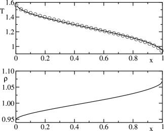
Figure 1: Nonequilibrium densities of a soft-point chain of length $L=512$ coupled to heat baths at temperatures $T_{L}=2$ and $T_{R}=0.5$. (upper panel) Temperature profile (solid curve); (lower panel) particle density profile. The circles in the upper panel have been obtained by assuming $T=5.5\ (1/\rho-\langle 1/\rho\rangle)+\langle T\rangle$.

Density and temperature profiles are qualitatively similar. This analogy was already noticed in Ref. Giberti and Rondoni (2011) for another model, where it was suggested that $T=C_{1}\rho^{-1}+C_{2}$, or, equivalently,

$$T(x)=C_{1}s(x)+C_{2}\;.$$ (11)

This intuition is here confirmed: the circles in the upper panel of Fig. 1 indeed correspond to the curve

$$T=5.5\ (s-\langle s\rangle)+\langle T\rangle$$ (12)

where the angular brackets denote an average along the chain. This relationship may be obtained from the state equation of the physical system, which can be written as $F(P,s,T)=0$, where $P$ denotes the pressure and the dependence on the volume is replaced by the equivalent dependence on $s$. Since the pressure is constant along the chain, a variation of the temperature transforms itself into a variation of $s$ and this variation is, in the limit of small displacements, linear. So one can write $F(P,s,T)=F(P,\langle s\rangle+\delta s,\langle T\rangle+\delta T)=F_{s}\delta s+F_{T}\delta T=0$, which is nothing but the formula proposed in Giberti and Rondoni (2011). The numerically determined coefficient $C_{1}=5.5$ corresponds to the ratio $F_{s}/F_{T}$, the two derivatives being determined in the middle point of the profile. We have thus identified the constants of that relation, which had not be done before, and we have confirmed that this relation does not correspond to Boyle law of perfect gases (since $C_{2}$ is not a small constant, cf. Giberti et al. (2019a)), although it implies that density is lower at higher temperatures. Note that Eq. (11) has been verified beyond the small displacement limit, which means that the conclusions of the above calculation can be generalized by integration of the infinitesimal variations.

For what concerns the fluxes, we find that the time averaged Lagrangian flux, $\overline{j}^{L}_{n}$, is independent of $n$ and approximately equal to $0.171$, while the time averaged Eulerian flux is independent of the threshold position $\theta$: $\overline{j}^{E}_{\theta}=\overline{j}^{D}_{\theta}+\overline{j}^{V}_{\theta}\approx 0.084+0.087=\overline{j}_{n}^{L}$. Therefore, the two definitions agree with one another, as they should. Moreover, we see that the conductive and convective contributions are approximately equal to one another for this choice of heat-bath temperatures. Below, in this section, we investigate the temperature dependence of the two contributions.

Now, we discuss the relationship between $\overline{j}^{L}_{n}$ and $\overline{j}^{D}_{\theta}$, as they follow from different ways of averaging the same quantity (compare Eq. (5) with Eq. (8)). A noticeable difference is that $\overline{j}^{L}_{n}$ refers to a fixed label $n$, irrespective of the position $q_{n}$, while $\overline{j}^{D}_{\theta}$ refers to a fixed threshold $\theta$, irrespective of the label $k$ of the adjacent particles sitting across the position $\theta$. It is therefore suggestive to compute conditional averages to bring the two definitions closer to one another. More precisely, we begin computing $\overline{J}^{L}_{k}(\xi)$ as the (time) average of $j^{L}_{k}$, under the condition that the center of mass $Q_{k}=(q_{k}+q_{k+1})/2$ is located inside the interval $[\xi-d\xi/2,\xi+d\xi/2]$ for a set of different fixed positions $\xi$. The results for $k=145$ and a chain of length 512 are shown in Fig. 2, (black diamonds) as a function of the scaled position $x=\xi/L$. We realize that $\overline{J}^{L}_{k}$ is independent of the particle position $\xi$, and equals the total flux (the fluctuations for relatively small and large $x$ values are due to poor statistics). One may conclude that this comes from the fact that the Lagrangian flux is the total flux, and that it does not depend on the label of the particle. However, the equality of the time averages is not trivial, as explained below, since $\overline{j}^{L}_{n}$ and $\overline{J}^{L}_{k}(\xi)$ can differ at all time instants $t$.

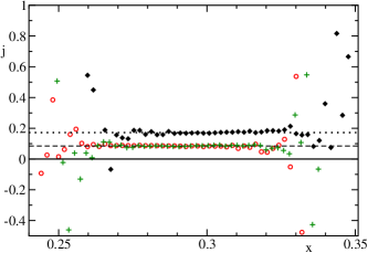
Figure 2: (Color online) Position dependence of the energy flux measured with different procedures in a chain of length 511 (same parameters as in Fig. 1). Black diamonds refer to the average Lagrangian flux $\overline{J}^{L}_{145}(\xi)$ conditioned to be measured at the scaled position $x=\xi/L$. Green plusses refer to the Lagrangian flux of the same particle, under the condition $xL\in[q_{145},q_{146}]$. Red circles refer to the average conductive component of the Eulerian flux measured in the location $153/L$, under the condition that the label of the contributing particle is $k$, for different $k$-values ($k$ is then mapped into an $x$-like variable via the stationary profile $x=\overline{q}_{k}/L$). The horizontal dashed and dotted lines correspond to the conductive Eulerian and Lagrangian flux, respectively.

Correspondingly, we have computed $\overline{J}_{y}^{D}(k)$, as the average of $j_{y}^{D}$, conditioned to a set of preassigned $k$ values ($k$ denoting the label such that $q_{k}<\xi<q_{k+1}$). The results are shown in Fig. 2 (red circles) for $x_{k}=153/512$. Since $\overline{J}^{L}_{k}(y)$ is a function of the position $y$, while $J^{D}_{y}(k)$ is a function of the label, for a meaningful comparison we have converted $k$ into $y$ by exploiting the knowledge of the average profile, i.e. from the knowledge of $y=\overline{q}_{k}$. From Fig. 2, we see that $J^{D}_{y}(k)$ too is constant and still equal to the conductive component of the heat flux. Therefore, it is not the combined dependence of the two quantities on $n$ and $y$ to be responsible for the observed differences between the Lagrangian flux and the conductive component of the Eulerian flux.

A third kind of conditional average helps to clarify the origin of the difference. Given an index value $m$, as normally done in the Lagrangian approach, we determine the average of all instantaneous flux values $j^{L}_{m}(t)$, counting only those events when $q_{m}<y<q_{m+1}$, no matter how close is the center of mass $Q_{m}$ of the pair $(q_{m}$, $q_{m+1})$ to the assigned threshold $y$ (as it was done in the computation of the diamonds). We call this observable $\tilde{J}(m,y)$; the results are displayed again in Fig. 2 for $m=145$ and different threshold values (see plusses). Once again this flux is independent of where the threshold is located. Less trivial is that the outcome of this third type of protocol now coincides with the conductive component of the Eulerian flux. We can therefore conclude that the subtle but important property which is responsible for the difference between $\overline{J}^{L}_{k}(y)$ and $\tilde{J}(k,y)$ is that in the first case the average is restricted to those moments when the center of mass is close to a given threshold, while in the second case, it is the matter of the threshold to be contained within the interval $[q_{k},q_{k+1}]$.

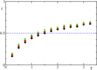
Figure 3: (Color online) Fraction $f=\langle j^{V}\rangle/\langle j^{L}\rangle$ versus the mean temperature $T=(T_{L}+T_{R})/2$, for three different chain lengths: $L=256$ (black dots), $L=512$ (red squares), and $L=1024$ (green triangles). In all cases $T_{L}-T_{R}=0.2$. The dashed horizontal line corresponds to an even distribution between conductive and convective component.

Having verified that the definitions given in the previous sections are meaningful, it is instructive to look at their relative size for different temperatures. In Fig. 3, we plot the fraction $f=\overline{j}^{V}/\overline{j}^{L}$ versus the average temperature $T=(T_{L}+T_{R})/2$ for three different chain lengths. This way, the scaling behavior of the flux with the system size does not matter and we can easily identify which contribution prevails. By definition, $0\leq f\leq 1$, the two extrema corresponding to a purely conductive ($f=0$) and a purely convective ($f=1$) flux. From Fig. 3, we see that at small temperatures, the convective components is relatively negligible in the SPC. In fact, it is reasonable to conjecture that $f(T)$ goes to zero for $T\to 0$, since the fluctuations of the particle around the equilibrium position decrease and so does the number of threshold crossings which contribute to the convective flux. A preliminary analysis suggests that the convective contribution vanishes linearly with $T$. On the other hand, at larger temperatures, the convective component becomes dominant, reflecting the wilder, increasingly gas-like behavior of the particles along the chain. Moreover, the ratio $f$ slowly grows with $L$ at fixed $T$. It probably saturates for $L\to\infty$, but more detailed numerical studies are necessary to test this hypothesis.

Finally, we look at temporal fluctuations. In order to average out the irrelevant microscopic fluctuations, it is convenient to look at the total flux. In the case of the Lagrangian approach, it is the matter of averaging $j^{L}_{n}$ over all $n$ values. In order to have a statistically equivalent definition of the Eulerian contribution, we have determined it for a set of equispaced thresholds, separated by the average inter particle distance.

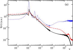
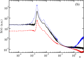
Figure 4: (Color online) Power spectrum of the heat flux for $L=1024$: panel a (b) refers to $T_{L}=0.3$ ($T_{L}=3.3$) and $T_{R}=0.2$ ($T_{R}=3.2$). The different curves correspond to the Lagrangian (black solid), Euler conductive (red dashed), and Euler convective (blue dotted) fluxes.

The results are plotted Fig. 4 for a relatively small and a large temperature. The peak exhibited by all curves correspond to time needed by a sound wave to propagate along the chain. Somehow surprisingly, stronger harmonics components are visible at lower temperatures, when the dynamics should in principle be more sinusoidal. It is also interesting to see that the spectral weight of the convective component prevails also at small temperatures (see the upper panel) where its average value is smaller than the conductive one (this can be extrapolated from the height of the power spectrum at extremely low frequencies).

III.2 Hard-point chain

We now study the energy flux in the HPC. The model, introduced and studied in Delfini et al. (2007), consists of a one-dimensional chain of $N$ particles of masses $\{m_{i}\}$, positions $\{q_{n}\}$ and linear momenta $\{p_{n}\}$ ordered along a line. Nearest neighbour particles interact through elastic collisions when $q_{n+1}-q_{n}=0$ (type-A collisions) and $q_{n+1}-q_{n}=a$ (type-B collisions) as given by the square–well potential in the relative distances defined by

$$V(q_{n+1}-q_{n})=\left\{\begin{array}[]{lll}0&,&\quad\mbox{$0\;<q_{n+1}-q_{n}\;<\;a$}\\ \infty&,&\quad\mbox{otherwise}\end{array}\right.$$ (13)

Type-B collisions can be visualised as if the particles were linked by an inextensible and massless string of fixed length $a$. Both types of collisions are of hard-core type, and are described by the same rule. Referring to the pair $(n,n+1)$, the particles’ momenta change as

$$p^{\prime}_{n} = \frac{m_{n}-m_{n+1}}{m_{n}+m_{n+1}}p_{n}+\frac{2m_{n}}{m_{n}+m_{n+1}}p_{n+1}$$ (14)

$$p^{\prime}_{n+1} = \frac{2m_{n+1}}{m_{n}+m_{n+1}}p_{n}-\frac{m_{n}-m_{n+1}}{m_{n}+m_{n+1}}p_{n+1}$$ (15)

where the primed momenta correspond to their values after a collision. To avoid ballistic energy transport, here we consider a diatomic chain for which the masses of the particles alternate between two different values that we chosen as $m_{n}=1$ for even $n$ and $m_{n}=\sqrt{2}$ for odd $n$.

The chain has fixed boundary conditions, meaning that for a chain of length $L$, we include two “virtual” particles with fixed positions $q_{0}=0$ and $q_{N}=L$. The chain length sets the specific volume $\alpha=L/N$, which is constrained to be $0<\alpha<a$ and determines the prevalence of type-A versus type-B collisions. The chain internal pressure $P$ is obtained as the average change of momentum due to the collisions, namely $P_{n}=p_{n}^{\prime}-p_{n}$. It is easy to note from Eq. (14) that the pressure is independent of the particle index, and thus homogeneous with respect to the position. The internal pressure $P$ is positive for $\alpha<a/2$ and negative for $\alpha>a/2$ Delfini et al. (2007). In what follows, and without loss of generality, we set the maximal particle distance to $a=1$.

The stationary nonequilibrium state is set by thermalising the particles next to the heat baths, namely $q_{1}$ and $q_{N}$, by means of a stochastic process. Each thermalized particle bears its own exponential clock; as the clock ticks the corresponding particle acquires a new velocity drawn from an equilibrium thermal state at the corresponding temperature ($T_{\rm L}$ or $T_{\rm R}$). We set the thermalisation rate to $10^{3}$. In between collisions and thermalisation, the particles move according to the HPC rules.

Temperature and particle density profiles are shown in Fig. 5 for $\alpha=0.3$. The temperature profile (upper panel) is similar to the one obtained for the SPC, though here we do not observe temperature discontinuities at the contacts with the heat baths. This is just a consequence of the stronger interaction assumed herein. However, given that the properties of the nonequilibrium state are determined by the bulk dynamics, the existence of a contact resistance is irrelevant. We also show the particle density (middle panel), computed as the inverse of the average inter particle distance $\rho$, which is equivalent to the number of particles per unit length. The equation of state for the HPC was derived in Delfini et al. (2007), and is given by

$$\rho(x)=\frac{T(x)}{P}-\frac{1}{\mathrm{e}^{P/T(x)}-1}\ ,$$ (16)

where $P$ is the internal pressure. The circles in the middle panel of Fig. 5, obtained through Eq. (16), show an excellent agreement. It is worthwhile noting that the equation of state governing the HPC local state differs from that of the SPC Eq. (11), except at small deviations from the mean density and kinetic temperature.

For $T_{L}\neq T_{R}$, the chain deforms inhomogeneously. We measure this deformation as the deviation of the average particle positions with respect to their equilibrium positions $q_{n}^{(\mathrm{eq})}$: $\Delta^{(\mathrm{eq})}(n)=\overline{q}_{n}-q_{n}^{(\mathrm{eq})}$. In the lowest panel of Fig. 5 we show $\Delta^{(\mathrm{eq})}$ for different values of $\alpha$. The deformation vanishes at the border due to the fixed boundary conditions; moreover, it is either positive or negative depending on the sign of the internal pressure. For $\alpha=1/2$, i.e. for zero pressure, $\Delta^{(\mathrm{eq})}=0$ along the chain. Finally, it looks like the maximal deformation exhibits a peak for intermediate specific volumes: this is an ”artifact” of the interaction scheme with the heat baths. In fact, for both $\alpha\to 0$ and $\alpha\to 1$, the average time separation between consecutive collisions goes to zero, i.e. the time scale of the HPC dynamics becomes arbitrarily short. On the other hand, the interaction with the heat bath being ruled by a fixed time scale, becomes increasingly weak.

A similar implication is found with reference to the energy flux that we are now going to discuss. We have implemented both the “Euler” and the “Lagrange” description as defined in section II. Once again, both currents have the same value, $j^{L}=j^{E}$, and do neither depend on the particle index nor on the physical position, as it must be. The dependence of the conductive and convective components of the heat flux on the specific volume $\alpha$ is illustrated in Fig. 6.

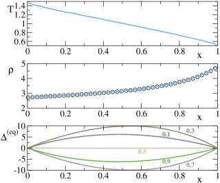
Figure 5: (Color online) Nonequilibrium densities of a hard-point chain consisting of $N=512$ particles, with temperature difference $T_{L}=1.5$, $T_{R}=0.5$ and $\alpha=0.3$. (upper panel) Temperature profile $T(x)$; (middle panel) particle density profile $\rho(x)$ (solid curve). The circles correspond to the particle density obtained from the temperature profile through the equation of state Eq.(16), with $P=2.4$ numerically computed as the momentum change due to collisions. (lower panel) Deformation of the chain $\Delta^{(\mathrm{eq})}$ for different values of $\alpha$ (as indicated by the labels).

There, we observe that the total flux is symmetric as a function of the parameter $\alpha$, about its value $1/2$. This is due to a duality linking the HPC models with specific volumes $\alpha$ and $\hat{\alpha}$, when $\hat{\alpha}=1-\alpha$. In fact, given the configuration I$=\{q_{1},q_{2},q_{3},\ldots,q_{L}\}$ with $q_{0}=0$ and $q_{L}=\alpha_{L}$, let us build the sister configuration II$=\{r_{0},r_{1},r_{2},\ldots,r_{L}\}$, starting from $r_{0}=(1-\alpha)L$, and recursively defining $r_{m+1}=r_{m}-1+(q_{L-m+1}-q_{L-m})$. Since the original length is $\alpha L$, the length of the new configuration is equal to $(1-\alpha)L$. Let us finally assume that the velocities of the configuration II are left unchanged: $\dot{r}_{m}=\dot{q}_{L-m}$.

Consider now two consecutive particles with positions $q_{n}$ and $q_{n+1}$ in the configuration I and assume that they are moving against one another. They will undergo a type-A collision after a time $\tau=d/(\dot{q}_{n+1}-\dot{q}_{n})$, where $d=q_{n+1}-q_{n}$ is the initial mutual distance. Within the sister configuration II, the corresponding particles of coordinate $r_{m}$, $r_{m+1}$ sit by construction at distance $1-d$ and move away from one another, as the ordering has been exchanged. Therefore, they will undergo a type-B collision after the same time $\tau$ as in the configuration I. Moreover, since the velocities are the same in the two configurations they remain equal after the collision. Analogously a collision of type-B in the first configuration is fully equivalent to a collision of type-A in the second one. We can therefore conclude that the initial relationship between the two configurations is maintained at all future times. In particular, one must expect that the energy flux is the same in both setups, as observed in Fig. 6.

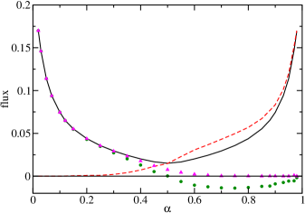
Figure 6: (Color online) Different fluxes for the HPC, as functions of the specific volume $\alpha$: total flux (black solid curve), Euler conductive flux (red dashed curve), Euler convective flux (green knots), and the contribution of type-A collisions to the flux (magenta triangles). All simulations are performed for a chain of length 1024, $T_{L}=1.5$, and $T_{R}=0.5$. The ratio between the two masses is 1.5. The distribution of interaction times with the heat bath is uniform between 0 and 2 in all cases.

As a second observation, we notice that the flux diverges for $\alpha\to 0$ (and then also for $\alpha\to 1$). Qualitatively, this is because the density increases and the time interval between consecutive collisions correspondingly decreases, tending to vanish. One may thus expect the flux to diverge as $1/\alpha$. However, the previously noticed decrease of the interaction strength, hence of the rate of thermalization, slows down such divergence.

From the definition of the fluxes in section II, one could naively expect that type-A and type-B collisions of the HPC are responsible for the convective and conductive flux, respectively. In fact, for $\alpha\to 0$, type-B collisions become increasingly rare, the dynamics is gas-like and the conductive flux vanishes. Analogously, for $\alpha\to 1$, type-A collisions disappear, the dynamics is crystal type and the convective component vanishes. However, Fig. 6, where the contribution of type-A collisions is reported (see the triangles), reveals that the agreement with the convective component only holds for $\alpha<1/2$.

For $\alpha>1/2$, the disagreement is not only quantitative, but even qualitative, since the contribution of type-A collisions stays positive, while the true convective component becomes even negative. This somehow surprising behavior is further investigated in the following section.

IV Role of pressure

From Fig. 6, we see that for $\alpha>1/2$, the convective component of the flux is negative, while the conductive component is consistently larger than the total flux to compensate for the negative convective contribution. It is plausible to conjecture that in the HPC the sign of the convective component of the flux is related to the sign of the pressure, since this latter observable changes sign precisely for $\alpha=1/2$. In order to test whether this is the general case, we have run some simulations with the SPC by varying the specific volume.

In the case of the SPC, when the specific volume $\alpha=1$ (equivalently the average particle distance) the repulsive and attractive force balance each other, and thus the chain at zero temperature is at equilibrium with zero pressure. Upon switching on the temperature, we expect the pressure to increase and this is what we see in Fig. 7, where the solid curve corresponds to the pressure as a function of the specific volume (see the left axis). Upon increasing $\alpha$ we expect at some point the pressure to change sign and this is what happens for $\alpha\approx 1.29$. In parallel to the computation of the pressure, we have determined also $j^{V}$ and $j^{D}$, finding that the convective component decreases and eventually changes sign as in the HPC. However, the change of sign does not occur at the same point ($j^{v}=0$ for $\alpha\approx 1.77$).

Therefore, although these simulations qualitatively confirm that decreasing the pressure contributes to decrease the convective component of the energy flux, which eventually becomes negative, a quantitative connection between the two observables is yet to be determined.

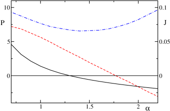
Figure 7: (Color online) Dependence of pressure (black curve, left labels) in the SPC on the specific volume $\alpha$. The blue dotted-dashed and red dashed curves refer to the convective and conductive components of the flux (see the right labels). Simulations have been performed in a a chain of $N=255$ particles, with $T_{L}=1.5$, and $T_{R}=0.5$; the collision times are uniformly distributed in the interval $[0.2,0.4]$.

V Concluding remarks

In this paper we have investigated different microscopic definitions of energy flux in 1D oscillators systems. In particular, we have considered two models (SPC and HPC) characterized by a repulsive potential, which preserves the particles order and a confining potential.

In both models, we have found that the Eulerian and Lagrangian fluxes are equal to one another as it should be. Concerning the conductive part $j_{\theta}^{D}$, we have observed that the conditional Lagrangian flux $\overline{J}^{L}_{k}$ equals the total flux, rather than $j_{\theta}^{D}$, despite the formal similarity of the two definitions. The reason has been found in the fact that the average $\overline{J}^{L}_{k}(y)$ is restricted to the instants of time in which the center of mass is close to a given threshold, while $\tilde{J}(k,y)$ is computed when the threshold is within the interval $[q_{k},q_{k+1}]$.

At small temperatures, the convective component $j_{\theta}^{V}$ is small, as one expects, but it becomes dominant at large tempreatures. This confirms an increasing similarity with a gas-like behaviour, which cannot be perfect if Eq. (12) extends to very high temperatures. We have also observed a small increase with the system size, which is probably a finite-size effect, but should be more thoroughly investigated.

The power spectra of the total flux show a peak in correspondence of the inverse of the time needed by a sound wave to propagate along the chain. Interestingly, stronger harmonic components appear at small temperatures, apparently contradicting the idea that the dynamics should then resemble that of harmonic oscillators. However, this peculiarity might be an instance of the long-range correlations produced by nonequilibrium boundary conditions (see, e.g., Ref. Giberti and Rondoni (2011)). An additional peculiarity is the relatively large amplitude of the spectrum of the covariant component even at small temperatures, when the average of $j^{V}$ is relatively small.

Rather surprisingly, in both the SPC and the HPC, we found that the convective component of the Eulerian flux tends to be negative in the presence of a negative pressure, thus making the conductive part larger than the total flux. At the moment, however, we have no indication of a quantitative relationship between negative conductive fluxes and negative pressures.

Finally, we have have shown that the symmetry of the heat flux (invariance under the transformation $\alpha\to 1-\alpha$) in the HPC, is a consequence of a duality of the model itself.

References

- Fourier (1822) J. Fourier, Théorie Analytique de la Chaleur (Didot, Berlin, 1822).
- Lepri (2016) S. Lepri, ed., Thermal Transport in Low Dimensions: From Statistical Physics to Nanoscale Heat Transfer (Lecture Notes in Physics), 1st ed. (Springer, 2016).
- Bonetto et al. (2000) F. Bonetto, J. L. Lebowitz, and L. Rey-Bellet, in Mathematical Physics 2000, edited by A. Fokas, A. Grigoryan, T. Kibble, and B. Zegarlinski (Imperial College, London, 2000) pp. 128–150.
- Lepri et al. (2005) S. Lepri, P. Sandri, and A. Politi, Eur. Phys. J. B 47, 549 (2005).
- Hurtado (2006) P. Hurtado, Phys. Rev. Lett. 96, 010601 (2006).
- Giberti et al. (2019a) C. Giberti, L. Rondoni, and C. Vernia, “Temperature and correlations in 1-dimensional systems,” (2019a), to appear.
- Giberti et al. (2019b) C. Giberti, L. Rondoni, and C. Vernia, “ fluctuations and lattice distortions in 1-dimensional systems,” (2019b), to appear.
- J.H.Irving and J.G.Kirkwood (1950) J.H.Irving and J.G.Kirkwood, J.Chem. Phys. 18, 817 (1950).
- Kubo et al. (2012) R. Kubo, M. Toda, and N. Hashitsume, Statistical Physics II: Nonequilibrium Statistical Mechanics, Springer Series in Solid-state Sciences (Springer Berlin Heidelberg, 2012).
- Lepri et al. (2003) S. Lepri, R. Livi, and A. Politi, Physics Reports 377, 1 (2003).
- Delfini et al. (2007) L. Delfini, S. Denisov, S. Lepri, R. Livi, P. Mohanty, and A. Politi, Eur. Phys. J. Special Topics 146, 21 (2007).
- Giberti and Rondoni (2011) C. Giberti and L. Rondoni, Phys. Rev. E 83, 041115 (2011).
- Note (1) Here and in the following we interchangeably refer to as to average distance or to specific volume.
- Note (2) The interaction between the system and the heat baths can be modelled through a deterministic thermostat, or by means of a stochastic process in which case the dynamics are Hamiltonian only in the bulk of the system.
- Note (3) Here and in the following, we assume to be constant, but a suitable time dependence can also be introduced, if deemed useful.
- Note (4) We implicitly assume that the particle positions are ordered from left to right and that the collisions do not modify their order.
- Note (5) The convective component is customarily used to compute the energy flux in billiard-like systems of interacting particles and it corresponds to the total Euler flux after requiring that local thermal equilibrium conditions holds Mejia-Monasterio et al. (2001); Larralde et al. (2002).
- Note (6) The overbar denotes time average.
- Mejia-Monasterio et al. (2001) C. Mejia-Monasterio, H. Larralde, and F. Leyvraz, Physical Review Letters 86, 5417 (2001).
- Larralde et al. (2002) H. Larralde, F. Leyvraz, and C. Mejia-Monasterio, Journal of Statistical Physics 113, 197 (2002).