Importance Weighted Hierarchical
Variational Inference

Abstract

Variational Inference is a powerful tool in the Bayesian modeling toolkit, however, its effectiveness is determined by the expressivity of the utilized variational distributions in terms of their ability to match the true posterior distribution. In turn, the expressivity of the variational family is largely limited by the requirement of having a tractable density function. To overcome this roadblock, we introduce a new family of variational upper bounds on a marginal log density in the case of hierarchical models (also known as latent variable models). We then give an upper bound on the Kullback-Leibler divergence and derive a family of increasingly tighter variational lower bounds on the otherwise intractable standard evidence lower bound for hierarchical variational distributions, enabling the use of more expressive approximate posteriors. We show that previously known methods, such as Hierarchical Variational Models, Semi-Implicit Variational Inference and Doubly Semi-Implicit Variational Inference can be seen as special cases of the proposed approach, and empirically demonstrate superior performance of the proposed method in a set of experiments.

1 Introduction

Bayesian Inference is an important statistical tool. However, exact inference is possible only in a small class of conjugate problems, and for many practically interesting cases, one has to resort to Approximate Inference techniques. Variational Inference (Hinton and van Camp, 1993; Waterhouse et al., 1996; Wainwright et al., 2008) being one of them is an efficient and scalable approach that gained a lot of interest in recent years due to advances in Neural Networks.

However, the efficiency and accuracy of Variational Inference heavily depend on how close an approximate posterior is to the true posterior. As a result, Neural Networks’ universal approximation abilities and great empirical success propelled a lot of interest in employing them as powerful sample generators (Nowozin et al., 2016; Goodfellow et al., 2014; MacKay, 1995) that are trained to output samples from approximate posterior when fed some standard noise as input. Unfortunately, a significant obstacle on this direction is a need for a tractable density $q(z\mid x)$, which in general requires intractable integration. A theoretically sound approach then is to give tight lower bounds on the intractable term – the differential entropy of $q(z|x)$, which is easy to recover from upper bounds on the marginal log-density. One such bound was introduced by Agakov and Barber (2004); however it’s tightness depends on the auxiliary variational distribution. Yin and Zhou (2018) suggested a multisample loss, whose tightness is controlled by the number of samples.

In this paper we consider hierarchical variational models (Ranganath et al., 2016; Salimans et al., 2015; Agakov and Barber, 2004) where the approximate posterior $q(z\mid x)$ is represented as a mixture of tractable distributions $q(z|\psi,x)$ over arbitrarily complicated mixing distribution $q(\psi|x)$: ${q(z|x)}=\int{q(z|\psi,x)}{q(\psi|x)}d\psi$. We show that such variational models contain semi-implicit models, first studied by Yin and Zhou (2018). To overcome the need for the closed-form marginal density $q(z|x)$ we then propose a novel family of tighter bounds on the marginal log-likelihood $\log p(x)$, which can be shown to generalize many previously known bounds: Hierarchical Variational Models (Ranganath et al., 2016) also known as auxiliary VAE bound (Maaløe et al., 2016), Semi-Implicit Variational Inference (Yin and Zhou, 2018) and Doubly Semi-Implicit Variational Inference (Molchanov et al., 2018). At the core of our work lies a novel variational upper bound on the marginal log-likelihood, which we combine with previously known lower bound (Burda et al., 2015) to give novel upper bound on the Kullback-Leibler (KL) divergence between hierarchical models, and apply it to the evidence lower bound (ELBO) to enable hierarchical approximate posteriors and/or priors. Finally, our method can be combined with the multisample bound of Burda et al. (2015) to tighten the marginal log-likelihood estimate further.

2 Background

Having a hierarchical model $p_{\theta}(x)=\int p_{\theta}(x\mid z)p_{\theta}(z)dz$ for observable objects $x$, we are interested in two tasks: inference and learning. The problem of Bayesian inference is that of finding the true posterior distribution $p_{\theta}(z\mid x)$, which is often intractable and thus is approximated by some $q_{\phi}(z\mid x)$. The problem of learning is that of finding parameters $\theta$ s.t. the marginal model distribution $p_{\theta}(x)$ approximates the true data-generating process of $x$ as good as possible, typically in terms of KL-divergence, which leads to the Maximum Likelihood Estimation problem.

Variational Inference provides a way to solve both tasks simultaneously by lower-bounding the intractable marginal log-likelihood $\log p_{\theta}(x)$ with the Evidence Lower Bound (ELBO) using the posterior approximation $q_{\phi}(z\mid x)$:

$$\log p_{\theta}(x)\geq\operatorname*{\mathbb{E}}_{q_{\phi}(z\mid x)}\log\frac{p_{\theta}(x,z)}{q_{\phi}(z\mid x)}.$$

The bound requires analytically tractable densities for both $q_{\phi}(z\mid x)$ and $p_{\theta}(z)$. The gap between the marginal log-likelihood and the bound is equal to $D_{KL}(q_{\phi}(z\mid x)\mid\mid p_{\theta}(z\mid x))$, which acts as a regularization preventing the true posterior $p(z|x)$ from deviating too far away from the approximate one $q(z|x)$, thus limiting the expressivity of the marginal distribution $p(x)$. Burda et al. (2015) proposed a family of tighter multisample bounds, generalizing the ELBO. We call it the IWAE bound:

$$\log p_{\theta}(x)\geq\operatorname*{\mathbb{E}}_{q_{\phi}(z_{1:M}\mid x)}\log\frac{1}{M}\sum_{m=1}^{M}\frac{p_{\theta}(x,z_{m})}{q_{\phi}(z_{m}\mid x)}.$$

Where from now on we write $q_{\phi}(z_{1:M}|x)=\prod_{m=1}^{M}q_{\phi}(z_{m}|x)$ for brevity. This bound has been shown (Domke and Sheldon, 2018) to be a tractable lower bound on ELBO for a variational distribution that has been obtained by a certain scoring procedure. However, the price of this increased tightness is higher computation complexity, especially in terms of the number of evaluations of the joint distribution $p_{\theta}(x,z)$, and thus we might want to come up with a more expressive posterior approximation to be used in the ELBO – a special case of $M=1$.

In the direction of improving the single-sample ELBO it was proposed (Agakov and Barber, 2004; Salimans et al., 2015; Maaløe et al., 2016; Ranganath et al., 2016) to use a hierarchical variational model (HVM) for $q(z\mid x)=\int{q(z\mid x,\psi)}{q(\psi\mid x)}d\psi$ with explicit joint density ${q(z,\psi\mid x)}$, where $\psi$ is auxiliary random variables. To overcome the intractability of the density ${q(z\mid x)}$, a variational lower bound on the ELBO is proposed. The tightness of the bound is controlled by the auxiliary variational distribution ${\tau(\psi\mid x,z)}$:

$$\log p_{\theta}(x)\geq\operatorname*{\mathbb{E}}_{q_{\phi}(z,\psi\mid x)}\left[\log p_{\theta}(x,z)-\log\frac{q_{\phi}(z,\psi\mid x)}{\tau(\psi\mid x,z)}\right]$$ (1)

Recently Yin and Zhou (2018) introduced semi-implicit models: hierarchical models $q(z\mid x)=\int q_{\phi}(z\mid\psi,x)q_{\phi}(\psi\mid x)d\psi$ with implicit but reparametrizable ${q_{\phi}(\psi\mid x)}$ and explicit ${q_{\phi}(z\mid\psi,x)}$, and suggested the following surrogate objective, which was later shown to be a lower bound (the SIVI bound) for all finite $K$ by Molchanov et al. (2018):

$$\log p_{\theta}(x)\geq\operatorname*{\mathbb{E}}_{q_{\phi}(z,\psi_{0}\mid x)}\operatorname*{\mathbb{E}}_{q_{\phi}(\psi_{1:K}\mid x)}\log\frac{p_{\theta}(x,z)}{\tfrac{1}{K+1}\sum_{k=0}^{K}q_{\phi}(z|\psi_{k},x)}$$ (2)

SIVI also can be generalized into a multisample bound similarly to the IWAE bound (Burda et al., 2015) in an efficient way by reusing samples $\psi_{1:K}$ for different $z_{m}$:

$$\log p(x)\geq\operatorname*{\mathbb{E}}\log\tfrac{1}{M}\sum_{m=1}^{M}\frac{p_{\theta}(x,z_{m})}{\tfrac{1}{K+1}\sum_{k=0}^{K}q_{\phi}(z_{m}|x,\psi_{m,k})}$$ (3)

Where the expectation is taken over ${q(\psi_{1:M,0},z_{1:M}\mid x)}$ and $\psi_{m,1:K}=\psi_{1:K}\sim q(\psi_{1:K}\mid x)$ is the same set of $K$ i.i.d. random variables for all $m$. Importantly, this estimator has $O(M+K)$ sampling complexity for $\psi$, unlike the naive approach, leading to $O(MK+M)$ sampling complexity. We will get back to this discussion in section 4.1.

2.1 SIVI Insights

Here we outline SIVI’s points of weaknesses and identify certain traits that make it possible to generalize the method and bridge it with the prior work.

First, note that both SIVI bounds (2) and (3) use samples from ${q_{\phi}(\psi_{1:K}\mid x)}$ to describe $z$, and in high dimensions one might expect that such "uninformed" samples would miss most of the time, resulting in near-zero likelihood ${q(z\mid\psi_{k},x)}$ and thus reducing the effective sample size. Therefore it is expected that in higher dimensions it would take many samples to accurately cover the regions high probability of $q(\psi\mid z,x)$ for the given $z$. Instead, ideally, we would like to target such regions directly while keeping the lower bound guarantees.

Another important observation that we’ll make use of is that many such semi-implicit models can be equivalently reformulated as a mixture of two explicit distributions: due to reparametrizability of $q_{\phi}(\psi\mid x)$ we have $\psi=g_{\phi}(\varepsilon\mid x)$ for some $\varepsilon\sim q(\varepsilon)$ with tractable density. We can then consider an equivalent hierarchical model $q_{\phi}(z)={\int q_{\phi}(z\mid g_{\phi}(\varepsilon\mid x),x)q(\varepsilon)d\varepsilon}$ that first samples $\varepsilon$ from some simple distribution, transforms this sample $\varepsilon$ into $\psi$ and then generates samples from $q_{\phi}(z\mid\psi,x)$. Thus from now on we’ll assume both $q_{\phi}(z\mid\psi,x)$ and $q_{\phi}(\psi\mid x)$ have tractable density, yet $q_{\phi}(z\mid\psi,x)$ can depend on $\psi$ in an arbitrarily complex way, making analytic marginalization intractable.

3 Importance Weighted Hierarchical Variational Inference

Having intractable $\log q_{\phi}(z\mid x)$ as a source of our problems, we seek a tractable and efficient upper bound, which is provided by the following theorem:

Theorem (Marginal log density upper bound).

For any $q(z,\psi\mid x)$, $K\in\mathbb{N}_{0}$ and $\tau(\psi\mid z,x)$ (under some regularity conditions) consider the following

$$\mathcal{U}_{K}=\operatorname*{\mathbb{E}}_{q(\psi_{0}\mid x,z)}\operatorname*{\mathbb{E}}_{\tau(\psi_{1:K}\mid z,x)}\log\left(\frac{1}{K+1}\sum_{k=0}^{K}\frac{q(z,\psi_{k}\mid x)}{\tau(\psi_{k}\mid z,x)}\right)$$

Then the following holds:

1. $\mathcal{U}_{K}\geq\log q(z\mid x)$

2. $\mathcal{U}_{K}\geq\mathcal{U}_{K+1}$

3. $\lim\limits_{K\to\infty}\mathcal{U}_{K}=\log q(z\mid x)$

Proof.

See Appendix for Theorem A.1. ∎

The proposed upper bound provides a variational alternative to MCMC-based upper bounds (Grosse et al., 2015) and complements the standard Importance Weighted stochastic lower bound of Burda et al. (2015) on the marginal log density:

$$\mathcal{L}_{K}=\operatorname*{\mathbb{E}}_{\tau(\psi_{1:K}\mid z,x)}\log\left(\frac{1}{K}\sum_{k=1}^{K}\frac{q(z,\psi_{k}\mid x)}{\tau(\psi_{k}\mid z,x)}\right)\leq\log q(z\mid x)$$

3.1 Upper Bound on KL divergence between hierarchical models

We now apply these bounds to marginal log-densities, appearing in KL divergence in case of both ${q(z|x)}=\int{q(z,\psi|x)}d\psi$ and $p(z)=\int{p(z,\zeta)}d\zeta$ being different (potentially structurally) hierarchical models. This results in a novel upper bound on KL divergence with auxiliary variational distributions $\tau(\psi\mid x,z)$ and $\rho(\zeta\mid z)$:

$$D_{KL}(q(z\mid x)\mid\mid\;p(z)) \leq\operatorname*{\mathbb{E}}_{q(z,\psi_{0}\mid x)}\operatorname*{\mathbb{E}}_{\tau(\psi_{1:K}\mid x,z)}\operatorname*{\mathbb{E}}_{\rho(\zeta_{1:L}\mid z)}\Biggl{[}\log\frac{\tfrac{1}{K+1}\sum_{k=0}^{K}\tfrac{q(z,\psi_{k}\mid x)}{\tau(\psi_{k}\mid x,z)}}{\tfrac{1}{L}\sum_{l=1}^{L}\frac{p(z,\zeta_{l})}{\rho(\zeta_{l}\mid z)}}\Biggr{]}$$ (4)

Crucially, in (4) we merged expectations over $q_{\phi}(z|x)$ and $q_{\phi}(\psi_{0}|x,z)$ into one expectation over the joint distribution $q_{\phi}(\psi_{0},z|x)$, which admits a more favorable factorization into ${q_{\phi}(\psi_{0}|x)q_{\phi}(z|x,\psi_{0})}$, and samples from the later are easy to simulate for the Monte Carlo-based estimation.

One can also give lower bounds in the same setting at (4). However, the main focus of this paper is on lower bounding the marginal log-likelihood, so we leave this discussion to appendix C.

3.2 Tractable lower bounds on marginal log-likelihood with hierarchical proposal

The proposed upper bound (4) allows us to lower bound the otherwise intractable ELBO in case of hierarchical $q(z\mid x)$ and $p(z)$, leading to Importance Weighted Hierarchical Variational Inference (IWHVI) lower bound:

$$\log p(x) \geq\operatorname*{\mathbb{E}}_{q(z\mid x)}\log\frac{p(x,z)}{q(z\mid x)}\geq\operatorname*{\mathbb{E}}_{q(z,\psi_{0}\mid x)}\operatorname*{\mathbb{E}}_{\tau(\psi_{1:K}\mid z,x)}\operatorname*{\mathbb{E}}_{\rho(\zeta_{1:L}\mid z)}\log\frac{p(x\mid z)\frac{1}{L}\sum_{k=1}^{L}\frac{p(z,\zeta_{l})}{\rho(\zeta_{l}\mid z)}}{\frac{1}{K+1}\sum_{k=0}^{K}\frac{q(z,\psi_{k}\mid x)}{\tau(\psi_{k}\mid z,x)}}$$ (5)

This bound introduces two additional auxiliary variational distributions $\rho$ and $\tau$ that are learned by maximizing the bound w.r.t. their parameters, tightening the bound. While the optimal distributions are $\tau(\psi\mid z,x)=q(\psi\mid z,x)$ and $\rho(\zeta\mid z)=p(\zeta\mid z)$, one can see that some particular choices of these distributions and hyperparameters $K,L$ render previously known methods like DSIVI, SIVI and HVM as special cases (see appendix B).

The bound (5) can be seen as variational generalization of SIVI (2) or multisample generalization of HVM (1). Therefore it has capacity to better estimate the true ELBO, reducing the gap and its regularizational effect, which should lead to more expressive variational approximations $q_{\phi}(z|x)$.

4 Multisample Extensions

Multisample bounds similar to the proposed one have already been studied extensively. In this section, we relate our results to such prior work.

4.1 Multisample Bound and Complexity

In this section we generalize the bound (5) further in a way similar to the IWAE multisample bound (Burda et al., 2015) (Theorem A.4), leading to the Doubly Importance Weighted Hierarchical Variational Inference (DIWHVI):

$$\log p(x)\geq\operatorname*{\mathbb{E}}\log\frac{1}{M}\sum_{m=1}^{M}\frac{p(x|z_{m})\frac{1}{L}\sum_{l=1}^{L}\frac{p(z_{m},\zeta_{m,l})}{\rho(\zeta_{m,l}\mid z_{m})}}{\frac{1}{K+1}\sum_{k=0}^{K}\frac{q(z_{m},\psi_{m,k}\mid x)}{\tau(\psi_{m,k}\mid z_{m},x)}}$$ (6)

Where the expectation is taken over the same generative process as in eq. 5, independently repeated $M$ times:

1. Sample $\psi_{m,0}\sim q(\psi\mid x)$ for $1\leq m\leq M$

2. Sample $z_{m}\sim q(z\mid x_{n},\psi_{m,0})$ for $1\leq m\leq M$

3. Sample $\psi_{m,k}\sim\tau(\psi\mid z_{m},x)$ for $1\leq m\leq M$ and $1\leq k\leq K$

4. Sample $\zeta_{m,l}\sim\rho(\zeta\mid z_{m})$ for $1\leq m\leq M$ and $1\leq l\leq L$

The price of the tighter bound (6) is quadratic sample complexity: it requires $M(1+K)$ samples of $\psi$ and $ML$ samples of $\zeta$. Unfortunately, the DIWHVI cannot benefit from the sample reuse trick of the SIVI that leads to the bound (3). The reason for this is that the bound (6) requires all terms in the outer denominator (the $\log q_{\phi}(z\mid x)$ estimate) to use the same distribution $\tau$, whereas by its very nature it should be very different for different $z_{m}$. A viable option, though, is to consider a multisample-conditioned ${\tau(\psi\mid z_{1:M})}$ that is invariant to permutations of $z$. We leave a more detailed investigation to a future work.

Runtime-wise when compared to the multisample SIVI (3) the DIWHVI requires additional $O(M)$ passes to generate $\tau(\psi\mid x,z_{m})$ distributions. However, since the SIVI requires a much larger number of samples $K$ to reach the same level of accuracy (see section 6.1) that are all then passed through a network to generate $q_{\phi}(z_{m}\mid x,\psi_{mk})$ distributions, the extra $\tau$ computation is likely to either bear a minor overhead, or be completely justified by reduced $K$. This is particularly true in the IWHVI case ($M=1$) where IWHVI’s single extra pass that generates $\tau(\psi|x,z)$ is dominated by $K+1$ passes that generate $q(z|x,\psi_{k})$.

4.2 Signal to Noise Ratio

Rainforth et al. (2018) have shown that multisample bounds (Burda et al., 2015; Nowozin, 2018) behave poorly during the training phase, having more noisy inference network’s gradient estimates, which manifests itself in decreasing Signal-to-Noise Ratio (SNR) as the number of samples increases. This raises a natural concern whether the same happens in the proposed model as $K$ increases. Tucker et al. (2019) have shown that upon a careful examination a REINFORCE-like (Williams, 1992) term can be seen in the gradient estimate, and REINFORCE is known for its typically high variance (Rezende et al., 2014). Authors further suggest to apply the reparametrization trick (Kingma and Welling, 2013) the second time to obtain a reparametrization-based gradient estimate, which is then shown to solve the decreasing SNR problem. The same reasoning can be applied to our bound, and we provide further details and experiments in appendix D, developing an IWHVI-DReG gradient estimator. We conclude that the problem of decreasing SNR exists in our bound as well, and is mitigated by the proposed gradient estimator.

4.3 Debiasing the bound

Nowozin (2018) has shown that the standard IWAE can be seen as a biased estimate of the marginal log-likelihood with the bias of order $O(1/M)$. They then suggested to use Generalized Jackknife of $d$-th order to reuse these $M$ samples and come up with an estimator with a smaller bias of order $O(1/M^{d})$ at the cost of higher variance and losing lower bound guarantees. Again, the same idea can be applied to our estimate; we leave further details to appendix E. We conclude that this way one can obtain better estimates of the marginal log-density, however since there is no guarantee that the obtained estimator gives an upper or a lower bound, we chose not to use it in experiments.

5 Related Work

More expressive variational distributions have been under an active investigation for a while. While we have focused our attention to approaches employing hierarchical models via bounds, there are many other approaches, roughly falling into two broad classes.

One possible approach is to augment some standard $q(z\mid x)$ with help of copulas (Tran et al., 2015), mixtures (Guo et al., 2016), or invertible transformations with tractable Jacobians also known as normalizing flows (Rezende and Mohamed, 2015; Kingma et al., 2016; Dinh et al., 2016; Papamakarios et al., 2017), all while preserving the tractability of the density. Kingma and Dhariwal (2018) have demonstrated that flow-based models are able to approximate complex high-dimensional distributions of real images, but the requirement for invertibility might lead to inefficiency in parameters usage and does not allow for abstraction as one needs to preserve dimensions.

An alternative direction is to embrace implicit distributions that one can only sample from, and overcome the need for tractable density using bounds or estimates (Huszár, 2017). Methods based on estimates (Mescheder et al., 2017; Shi et al., 2017), for example, via the Density Ratio Estimation trick (Goodfellow et al., 2014; Uehara et al., 2016; Mohamed and Lakshminarayanan, 2016), typically estimate the densities indirectly utilizing an auxiliary critic and hide dependency on variational parameters $\phi$, hence biasing the optimization procedure. Titsias and Ruiz (2018) have shown that in the gradient-based ELBO optimization in case of a hierarchical model with tractable $q_{\phi}(z\mid\psi)$ and $q_{\phi}(\psi)$ one does not need the marginal log density $\log q_{\phi}(z\mid x)$ per se, only its gradient, which can be estimated using MCMC. Major disadvantage of these methods is that they either lose bound guarantees or make its evaluation intractable and thus cannot be combined with multisample bounds during the evaluation phase.

The core contribution of the paper is a novel upper bound on marginal log-likelihood. Previously, Dieng et al. (2017); Kuleshov and Ermon (2017) suggested using $\chi^{2}$-divergence to give a variational upper bound to the marginal log-likelihood. However, their bound was not an expectation of a random variable, but instead a logarithm of the expectation, preventing unbiased stochastic optimization. Jebara and Pentland (2001) reverse Jensen’s inequality to give a variational upper bound in case of mixtures of exponential family distributions by extensive use of the problem’s structure. Related to our core idea of joint sampling $z$ and $\psi_{0}$ in (4) is an observation of Grosse et al. (2015) that Annealed Importance Sampling (AIS, Neal (2001)) ran backward from the auxiliary variable sample $\psi_{0}$ gives an unbiased estimate of $1/q(z\mid x)$, and thus can also be used to upper bound the marginal log-density. However, AIS-based estimation is too computationally expensive to be used during training.

6 Experiments

We only focus on cases with explicit prior $p(z)$ to simplify comparison to prior work. Hierarchical priors correspond to nested variational inference, to which most of the variational inference results readily apply (Atanov et al., 2019).

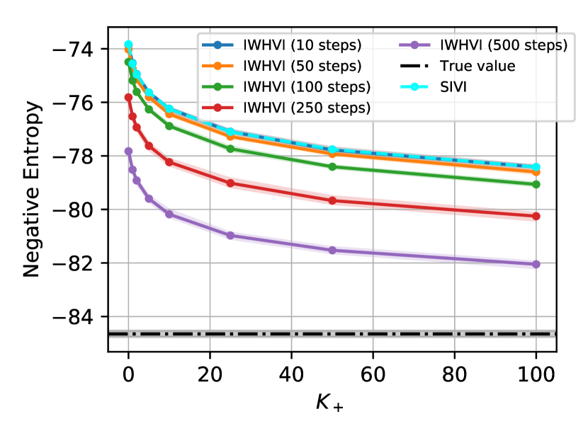
(a) Negative entropy bounds for 50-dimensional Laplace distribution. Shaded area denotes 90% confidence interval computed over 50 independent runs for each $K$.

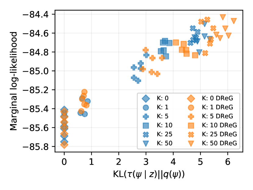
(b) Final marginal log-likelihood $\log p(x)$ estimates and expected $D_{KL}(\tau(\psi\mid z)\mid\mid q(\psi))$ for IWHVI-based VAEs trained with different $K$. Each model was trained and plotted 6 times.

6.1 Toy Experiment

As a toy experiment we consider a 50-dimensional factorized standard Laplace distribution $q(z)$ as a hierarchical scale-mixture model:

$$q(z)=\prod_{d=1}^{50}\text{Laplace}(z_{d}\mid 0,1)=\int\prod_{d=1}^{50}\mathcal{N}(z_{d}\mid 0,\psi_{d})\text{Exp}(\psi_{d}\mid\tfrac{1}{2})d\psi_{1:50}$$

We do not make use of factorized joint distribution $q(z,\psi)$ to explore bound’s behavior in high dimensions. We use the proposed bound from Theorem A.1 and compare it to SIVI (Yin and Zhou, 2018) on the task of upper-bounding the negative differential entropy $\operatorname*{\mathbb{E}}_{q(z)}\log q(z)$. For IWHVI we take $\tau(\psi\mid z)$ to be a Gamma distribution whose concentration and rate are generated by a neural network with three 500-dimensional hidden layers from $z$. We use the freedom to design architecture and initialize the network at prior. Namely, we also add a sigmoid "gate" output with large initial negative bias and use the gate to combine prior concentration and rate with those generated by the network. This way we are guaranteed to perform no worse than SIVI even at a randomly initialized $\tau$. Figure 1(a) shows the value of the bound for a different number of optimization steps over $\tau$ parameters, minimizing the bound. The whole process (including random initialization of neural networks) was repeated 50 times to compute empirical 90% confidence intervals. As results clearly indicate, the proposed bound can be made much tighter, more than halving the gap to the true negative entropy.

6.2 Variational Autoencoder

Method	MNIST	OMNIGLOT
From (Mescheder et al., 2017)
AVB + AC	$-83.7\pm 0.3$	—
IWHVI	$-83.9\pm 0.1$	$-104.8\pm 0.1$
SIVI	$-84.4\pm 0.1$	$-105.7\pm 0.1$
HVM	$-84.9\pm 0.1$	$-105.8\pm 0.1$
VAE + RealNVP	$-84.8\pm 0.1$	$-106.0\pm 0.1$
VAE + IAF	$-84.9\pm 0.1$	$-107.0\pm 0.1$
VAE	$-85.0\pm 0.1$	$-106.6\pm 0.1$

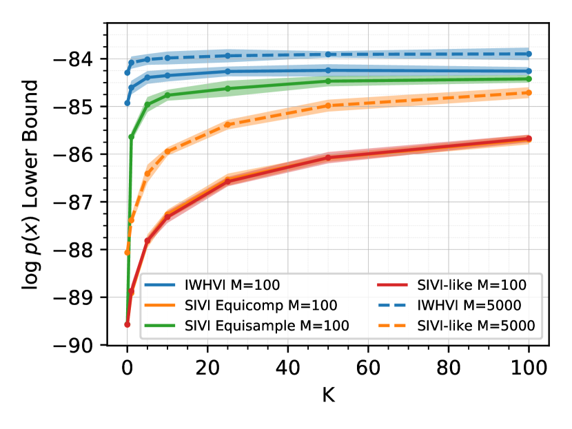
Figure 2: Left: Test log-likelihood on dynamically binarized MNIST and OMNIGLOT. Right: Comparison of multisample DIWHVI and SIVI-IW on a trained MNIST VAE from section 6.2 for $M=100$ and $5000$. Shaded area denotes $\pm 2$ std. interval, computed over 10 independent runs for each value of $K$.

We further test our method on the task of generative modeling, applying it to VAE (Kingma and Welling, 2013), which is a standard benchmark for inference methods. Ideally, better inference should allow one to learn more expressive generative models. We report results on two datasets: MNIST (LeCun et al., 1998) and OMNIGLOT (Lake et al., 2015). For MNIST we follow the setup by Mescheder et al. (2017), and for OMNIGLOT we follow the standard setup (Burda et al., 2015). For experiment details see appendix F.

During training we used the proposed bound eq. 5 with analytically tractable prior $p(z)=\mathcal{N}(z\mid 0,1)$ with increasing number $K$: we used $K=0$ for the first 250 epochs, $K=5$ for the next 250 epochs, and $K=25$ for the next 500 epochs, and $K=50$ from then on. We used $M=1$ during training.

To estimate the marginal log-likelihood for hierarchical models (IWHVI, SIVI, HVM) we use the DIWHVI lower bound (6) for $M=5000$, $K=100$ (for justification of DIWHVI as an evaluation metric see section 6.3). Results are shown in fig. 2. To evaluate the SIVI using the DIWHVI bound we fit $\tau$ to a trained model by making 7000 epochs on the trainset with $K=50$, keeping parameters of $q_{\phi}(z,\psi\mid x)$ and $p_{\theta}(x,z)$ fixed. We observed improved performance compared to special cases of HVM and SIVI, and the method showed comparable results to the prior works.

For HVM on MNIST we observed its $\tau(\psi\mid z)$ essentially collapsed to $q(\psi)$, having expected KL divergence between the two extremely close to zero. This indicates the "posterior collapse" (Kim et al., 2018; Chen et al., 2016) problem where the inference network $q(z\mid\psi)$ chose to ignore the extra input $\psi$ and effectively degenerated to a vanilla VAE. At the same time IWHVI does not suffer from this problem due to non-zero $K$, achieving average $D_{KL}({\tau(\psi\mid z,x)}\mid\mid{q(\psi)})$ of approximately 6.2 nats, see section 6.3. For OMNIGLOT HVM did learn useful $\tau$, and achieved average $D_{KL}({\tau(\psi\mid z,x)}\mid\mid{q(\psi)})\approx 1.98$ nats, however IWHVI did much better and achieved $\approx 9.97$ nats.

To investigate $K$’s influence on the training process, we trained VAEs on MNIST for 3000 epochs for different values of $K$ and evaluated DIWHVI bound for $M=1000,K=100$ and plotted results in fig. 1(b). One can see that higher values of $K$ lead to better final models in terms of marginal log-likelihood, as well as more informative auxiliary inference networks $\tau(\psi\mid z,x)$ compared to the prior $q(\psi)$. Using IWHVI-DReG gradient estimator (see appendix D) increased the KL divergence, but resulted in only a modest increase in the marginal log-likelihood.

6.3 DIWHVI as Evaluation Metric

One of the established approaches to evaluate the intractable marginal log-likelihood in Latent Variable Models is to compute the multisample IWAE-bound with large $M$ since it is shown to converge to the marginal log-likelihood as $M$ goes to infinity. Since both IWHVI and SIVI allow tightening the bound by taking more samples $z_{m}$, we compare methods along this direction.

Both DIWHVI and SIVI (being a special case of the former) can be shown to converge to marginal log-likelihood as both $M$ and $K$ go to infinity, however, rates might differ. We empirically compare the two by evaluating an MNIST-trained IWHVAE model from section 6.2 for several different values $K$ and $M$. We use the proposed DIWHVI bound (6), and compare it with several SIVI modifications. We call SIVI-like the (6) with $\tau(\psi\mid z)=q(\psi)$, but without $\psi$ reuse, thus using $MK$ independent samples. SIVI Equicomp stands for sample reusing bound (3), which uses only $M+K$ samples, and uses same $\psi_{1:K}$ for every $z_{m}$. SIVI Equisample is a fair comparison in terms of the number of samples: we take $M(K+1)$ samples of $\psi$, and reuse $MK$ of them for every $z_{m}$. This way we use the same number of samples $\psi$ as DIWHVI does, but perform $O(M^{2}K)$ log-density evaluations to estimate $\log q(z\mid x)$, which is why we only examine the $M=100$ case.

Results shown in fig. 2 indicate superior performance of the DIWHVI bound. Surprisingly SIVI-like and SIVI Equicomp estimates nearly coincide, with no significant difference in variance; thus we conclude sample reuse does not hurt SIVI. Still, there is a considerable gap to the IWHVI bound, which uses similar to SIVI-like amount of computing and samples. In a more fair comparison to the Equisample SIVI bound, the gap is significantly reduced, yet IWHVI is still a superior bound, especially in terms of computational efficiency, as there are no $O(M^{2}K)$ operations.

Comparing IWHVI and SIVI-like for $M=5000$ we see that the former converges after a few dozen samples, while SIVI is rapidly improving, yet lagging almost 1 nat behind for 100 samples, and even 0.5 nats behind the HVM bound (IWHVI for $K=0$). One explanation for the observed behaviour is large $\mathbb{E}_{q(z\mid x)}D_{KL}(q(\psi\mid x)\mid\mid q(\psi\mid x,z))$, which was estimated (on a test set) to be at least $46.85$ nats, causing many samples from $q(\psi)$ to generate poor likelihood $q(z\mid\psi)$ for a given $z_{m}$ due to large difference with the true inverse model $q(\psi\mid x,z)$. This is consistent with motivation layed out in section 2.1: a better approximate inverse model $\tau$ leads to more efficient sample usage. At the same time $\mathbb{E}_{q(z\mid x)}D_{KL}(\tau(\psi\mid x,z)\mid\mid q(\psi\mid x,z))$ was estimated to be approximately $3.24$ and $\mathbb{E}_{q(z\mid x)}D_{KL}(\tau(\psi\mid x,z)\mid\mid q(\psi\mid x))\approx 6.25$, proving that one can indeed do much better by learning $\tau(\psi\mid x,z)$ instead of using the prior $q(\psi\mid x)$.

7 Conclusion

We presented a variational upper bound on the marginal log density, which allowed us to formulate sandwich bounds for $D_{KL}(q(z\mid x)\mid\mid p(z))$ for the case of hierarchical model $q(z\mid x)$ in addition to prior works that only provided multisample variational upper bounds for the case of $p(z$ being a hierarchical model. We applied it to lower bound the intractable ELBO with a tractable one for the case of latent variable model approximate posterior $q_{\phi}(z\mid x)$. We experimentally validated the bound and showed it alleviates regularizational effect to a further extent than prior works do, allowing for more expressive approximate posteriors, which does translate into a better inference. We then combined our bound with multisample IWAE bound, which led to a tighter lower bound of the marginal log-likelihood. We therefore believe the proposed variational inference method will be useful for many variational models.

Appendix A Proofs

Theorem A.1 (Marginal log-density upper bound).

For any $q(z,\psi)$, $K\in\mathbb{N}_{0}$ and $\tau(\psi\mid z)$ such that for any $\psi$ s.t. $\tau(\psi\mid z)=0$ we have $q(\psi,z)=0$, consider

$$\mathcal{U}_{K}=\operatorname*{\mathbb{E}}_{q(\psi_{0}\mid z)}\operatorname*{\mathbb{E}}_{\tau(\psi_{1:K}\mid z)}\log\left(\frac{1}{K+1}\sum_{k=0}^{K}\frac{q(z,\psi_{k})}{\tau(\psi_{k}\mid z)}\right)$$

where we write $\tau(\psi_{1:K}\mid z)=\prod_{k=1}^{K}\tau(\psi_{k}\mid z)$ for brevity. Then the following holds:

1. $\mathcal{U}_{K}\geq\log q(z)$

2. $\mathcal{U}_{K}\geq\mathcal{U}_{K+1}$

3. $\lim\limits_{K\to\infty}\mathcal{U}_{K}=\log q(z)$.

Proof.

1. Consider a gap between the proposed bound at the marginal log density:

   Gap $$=\operatorname*{\mathbb{E}}_{q(\psi_{0}\mid z)}\operatorname*{\mathbb{E}}_{\tau(\psi_{1:K}\mid z)}\log\left(\frac{1}{K+1}\sum_{k=0}^{K}\frac{q(z,\psi_{k})}{\tau(\psi_{k}\mid z)}\right)-\log q(z)$$

   $$=\operatorname*{\mathbb{E}}_{q(\psi_{0}\mid z)}\operatorname*{\mathbb{E}}_{\tau(\psi_{1:K}\mid z)}\log\left(\frac{1}{K+1}\sum_{k=0}^{K}\frac{q(\psi_{k}\mid z)}{\tau(\psi_{k}\mid z)}\right)$$

   $$=\operatorname*{\mathbb{E}}_{q(\psi_{0}\mid z)}\operatorname*{\mathbb{E}}_{\tau(\psi_{1:K}\mid z)}\log\left(\frac{q(\psi_{0}\mid z)\tau(\psi_{1:K}\mid z)}{\omega_{q,\tau}(\psi_{0:K}\mid z)}\right)$$

   $$=D_{KL}(q(\psi_{0}\mid z)\tau(\psi_{1:K}\mid z)\mid\mid\omega_{q,\tau}(\psi_{0:K}\mid z))\geq 0$$

   Where the last line holds due to $\omega_{q}$ being a normalized density function (see Lemma A.2):

   $$\omega_{q,\tau}(\psi_{0:K}\mid z)=\frac{q(\psi_{0}\mid z)\tau(\psi_{1:K}\mid z)}{\frac{1}{K+1}\sum_{k=0}^{K}\frac{q(\psi_{k}\mid z)}{\tau(\psi_{k}\mid z)}}$$

2. Now we will prove the second claim.

   $$\mathcal{U}_{K}-\mathcal{U}_{K+1} =\operatorname*{\mathbb{E}}_{q(\psi_{0}\mid z)}\operatorname*{\mathbb{E}}_{\tau(\psi_{1:K+1}\mid z)}\log\frac{\frac{1}{K+1}\sum_{k=0}^{K}\frac{q(z,\psi_{k})}{\tau(\psi_{k}\mid z)}}{\frac{1}{K+2}\sum_{k=0}^{K+1}\frac{q(z,\psi_{k})}{\tau(\psi_{k}\mid z)}}$$

   $$=\operatorname*{\mathbb{E}}_{q(\psi_{0}\mid z)}\operatorname*{\mathbb{E}}_{\tau(\psi_{1:K+1}\mid z)}\log\frac{q(\psi_{0}\mid z)\tau(\psi_{1:K+1}\mid z)}{\nu_{q,\tau}(\psi_{0:K+1}\mid z)}$$

   $$=D_{KL}\left(q(\psi_{0}\mid z)\tau(\psi_{1:K+1}\mid z)\mid\mid\nu_{q,\tau}(\psi_{0:K+1}\mid z)\right)\geq 0$$

   Where we used the fact that $\nu_{q,\tau}(\psi_{0:K+1}\mid z)$ is normalized density due to Lemma A.3

   $$\nu_{q,\tau}(\psi_{0:K+1}\mid z)=\omega_{q,\tau}(\psi_{0:K}\mid z)\tau(\psi_{K+1}\mid z)\frac{1}{K+2}\sum_{k=0}^{K+1}\frac{q(\psi_{k}\mid z)}{\tau(\psi_{k}\mid z)}$$

3. For the last claim we follow (Burda et al., 2015). Consider

   $$M_{K}=\frac{1}{K+1}\sum_{k=0}^{K}\frac{q(z,\psi_{k})}{\tau(\psi_{k}\mid z)}=\overbrace{\frac{1}{K+1}\frac{q(z,\psi_{0})}{\tau(\psi_{0}\mid z)}}^{A_{K}}+\overbrace{\frac{K}{K+1}}^{B_{K}}\overbrace{\frac{1}{K}\sum_{k=1}^{K}\frac{q(z,\psi_{k})}{\tau(\psi_{k}\mid z)}}^{X_{K}}$$

   Due to Law of Large Numbers we have

   $$A_{K}\xrightarrow[K\to\infty]{a.s.}0,\quad\quad X_{K}\xrightarrow[K\to\infty]{a.s.}\operatorname*{\mathbb{E}}_{\tau(\psi\mid z)}\frac{q(z,\psi)}{\tau(\psi\mid z)}=q(z),\quad\quad B_{K}\xrightarrow[K\to\infty]{a.s.}1$$

   Thus

   $$M_{K}\xrightarrow[K\to\infty]{a.s.}q(z),\quad\quad\mathcal{U}_{K}=\operatorname*{\mathbb{E}}_{\tau(\psi_{0:K}\mid z)}\log M_{K}\xrightarrow[K\to\infty]{}\log q(z)$$

∎

Lemma A.2 ($\omega_{q,\tau}$ distribution, following Domke and Sheldon (2018)).

Given $z$, consider a following generative process:

• Sample $K+1$ i.i.d. samples from $\hat{\psi}_{k}\sim\tau(\psi\mid z)$

• For each sample compute its weight $w_{k}=\frac{q(\hat{\psi}_{k},z)}{\tau(\hat{\psi}_{k}\mid z)}$

• Sample $h\sim\text{Cat}\left(\frac{w_{0}}{\sum_{k=0}^{K}w_{k}},\dots,\frac{w_{K}}{\sum_{k=0}^{K}w_{k}}\right)$

• Put $h$-th sample first, and then the rest: $\psi_{0}=\hat{\psi}_{h}$, $\psi_{1:K}=\hat{\psi}_{\backslash h}$

Then the marginal density of $\psi_{0:K}$

$$\omega_{q,\tau}(\psi_{0:K}\mid z)=\frac{q(\psi_{0}\mid z)\tau(\psi_{1:K}\mid z)}{\frac{1}{K+1}\sum_{k=0}^{K}\frac{q(\psi_{k}\mid z)}{\tau(\psi_{k}\mid z)}}$$

Proof.

The joint density for the generative process described above is

$$\omega_{q,\tau}(\hat{\psi}_{0:K},h,\psi_{0:K}\mid z)=\tau(\hat{\psi}_{0:K}\mid z)\tfrac{w_{h}}{\sum_{k=0}^{K}w_{k}}\delta(\psi_{0}-\hat{\psi}_{h})\delta(\psi_{1:K}-\hat{\psi}_{\backslash h})$$

One can see that this is indeed a normalized density

$$\int\sum_{h=0}^{K} \left(\int\omega_{\tau}(\hat{\psi}_{0:K},h,\psi_{0:K}\mid z)d\psi_{0:K}\right)d\hat{\psi}_{0:K}=\int\sum_{h=0}^{K}\tau(\hat{\psi}_{0:K}\mid z)\tfrac{w_{h}}{\sum_{k=0}^{K}w_{k}}d\hat{\psi}_{0:K}$$

$$=\int\tau(\hat{\psi}_{0:K}\mid z)\sum_{h=0}^{K}\tfrac{w_{h}}{\sum_{k=0}^{K}w_{k}}d\hat{\psi}_{0:K}=\int\tau(\hat{\psi}_{0:K}\mid z)d\hat{\psi}_{0:K}=1$$

The marginal density $\omega_{q,\tau}(\psi_{0:K}\mid z)$ then is

$$\omega_{q,\tau}(\psi_{0:K}\mid z) =\int\sum_{h=0}^{K}\tau(\hat{\psi}_{0:K}\mid z)\tfrac{w_{h}}{\sum_{k=0}^{K}w_{k}}\delta(\psi_{0}-\hat{\psi}_{h})\delta(\psi_{1:K}-\hat{\psi}_{\backslash h})d\hat{\psi}_{0:K}$$

$$=(K+1)\int\tau(\hat{\psi}_{0:K}\mid z)\tfrac{w_{0}}{\sum_{k=0}^{K}w_{k}}\delta(\psi_{0}-\hat{\psi}_{0})\delta(\psi_{1:K}-\hat{\psi}_{1:K})d\hat{\psi}_{0:K}$$

$$=\int\tau(\hat{\psi}_{1:K}\mid z)\tfrac{q(z,\hat{\psi}_{0})}{\tfrac{1}{K+1}\sum_{k=0}^{K}w_{k}}\delta(\psi_{0}-\hat{\psi}_{0})\delta(\psi_{1:K}-\hat{\psi}_{1:K})d\hat{\psi}_{0:K}$$

$$=\tau(\psi_{1:K}\mid z)\tfrac{q(z,\psi_{0})}{\tfrac{1}{K+1}\sum_{k=0}^{K}\tfrac{q(\psi_{k},z)}{\tau(\psi_{k}\mid z)}}=\tfrac{q(\psi_{0}\mid z)\tau(\psi_{1:K}\mid z)}{\tfrac{1}{K+1}\sum_{k=0}^{K}\tfrac{q(\psi_{k}\mid z)}{\tau(\psi_{k}\mid z)}}$$

Where on the second line we used the fact that integrand is symmetric under the choice of $h$.

∎

Lemma A.3.

Let

$$\nu_{q,\tau}(\psi_{0:K+1}\mid z)=\omega_{q,\tau}(\psi_{0:K}\mid z)\tau(\psi_{K+1}\mid z)\frac{1}{K+2}\sum_{k=0}^{K+1}\frac{q(\psi_{k}\mid z)}{\tau(\psi_{k}\mid z)}$$

Then $\nu_{q,\tau}(\psi_{0:K+1}\mid z)$ is a normalized density.

Proof.

$\nu_{q,\tau}(\psi_{0:K+1}\mid z)$ is non-negative due to all the terms being non-negative. Now we’ll show it integrates to 1 (colors denote corresponding terms):

$$\int \omega_{q,\tau}(\psi_{0:K}\mid z){\color[rgb]{0,0,1}\tau(\psi_{K+1}\mid z)}{\color[rgb]{1,0,0}\frac{1}{K+2}\sum_{k=0}^{K+1}\frac{q(\psi_{k}\mid z)}{\tau(\psi_{k}\mid z)}}d\psi_{0:K+1}$$

$$={\color[rgb]{1,0,0}\frac{1}{K+2}}{\color[rgb]{.5,0,.5}\int\omega_{q,\tau}(\psi_{0:K}\mid z)}\left[{\color[rgb]{1,0,0}\sum_{k=0}^{K}\frac{q(\psi_{k}\mid z)}{\tau(\psi_{k}\mid z)}+{\color[rgb]{0,0,1}\int\tau(\psi_{K+1}\mid z)}\frac{q(\psi_{K+1}\mid z)}{\tau(\psi_{K+1}\mid z)}}{\color[rgb]{0,0,1}d\psi_{K+1}}\right]d\psi_{0:K}$$

$$=\frac{1}{K+2}\left[\int{\color[rgb]{.5,0,.5}\frac{q(\psi_{0}\mid z)\tau(\psi_{1:K}\mid z)}{\frac{1}{\color[rgb]{1,.5,0}K+1}\sum_{k=0}^{K}\frac{q(\psi_{k}\mid z)}{\tau(\psi_{k}\mid z)}}}\sum_{k=0}^{K}\frac{q(\psi_{k}\mid z)}{\tau(\psi_{k}\mid z)}d\psi_{0:K}+1\right]=\frac{{\color[rgb]{1,.5,0}K+1}+1}{K+2}=1$$

∎

Theorem A.4 (DIWHVI Evidence Lower Bound).

$$\log p(x)\geq\operatorname*{\mathbb{E}}\log\left[\frac{1}{M}\sum_{m=1}^{M}\frac{p(x\mid z_{m})\frac{1}{K}\sum_{k=1}^{K}\frac{p(z_{m},\zeta_{m,k})}{\rho(\zeta_{m,k}\mid z_{m})}}{\frac{1}{K+1}\sum_{k=0}^{K}\frac{q(z_{m},\psi_{m,k}\mid x)}{\tau(\psi_{m,k}\mid z_{m},x)}}\right]$$ (7)

Where the expectation is taken over the following generative process:

1. Sample $\psi_{m,0}\sim q(\psi\mid x)$ for $1\leq m\leq M$

2. Sample $z_{m}\sim q(z\mid x_{n},\psi_{m,0})$ for $1\leq m\leq M$

3. Sample $\psi_{m,k}\sim\tau(\psi\mid z_{m},x)$ for $1\leq m\leq M$ and $1\leq k\leq K$

4. Sample $\zeta_{m,k}\sim\rho(\zeta\mid z_{m})$ for $1\leq m\leq M$ and $1\leq k\leq K$

Proof.

Consider a random variable

$$X_{M}=\frac{1}{M}\sum_{m=1}^{M}\frac{p(x\mid z_{m})\frac{1}{K}\sum_{k=1}^{K}\frac{p(z_{m},\zeta_{m,k})}{\rho(\zeta_{m,k}\mid z_{m})}}{\frac{1}{K+1}\sum_{k=0}^{K}\frac{q(z_{m},\psi_{m,k}\mid x)}{\tau(\psi_{m,k}\mid z_{m},x)}}$$

We’ll show it’s an unbiased estimate of $p(x)$ (colors denote corresponding terms) and then just invoke Jensen’s inequality:

$$\operatorname*{\mathbb{E}}X_{M} =\int\Biggl{[}\left(\prod_{m=1}^{M}q(\psi_{m,0}\mid x)q(z_{m}\mid\psi_{m,0},x)\tau(\psi_{m,1:K}\mid z_{m},x){\color[rgb]{1,0,0}\rho(\zeta_{m,1:K}\mid z_{m})}\right)$$

$$\quad\quad\quad\frac{1}{M}\sum_{m=1}^{M}\frac{p(x\mid z_{m}){\color[rgb]{1,0,0}\frac{1}{K}\sum_{k=1}^{K}\frac{p(z_{m},\zeta_{m,k})}{\rho(\zeta_{m,k}\mid z_{m})}}}{\frac{1}{K+1}\sum_{k=0}^{K}\frac{q(z_{m},\psi_{m,k}\mid x)}{\tau(\psi_{m,k}\mid z_{m},x)}}\Biggr{]}d\psi_{1:M,0:K}d\zeta_{1:M,1:K}dz_{1:M}$$

First, we move in the integral w.r.t. $\zeta$ into the numerator:

$$\phantom{\operatorname*{\mathbb{E}}X_{M}}=\int\Biggl{(}\frac{1}{M}\sum_{m=1}^{M} \frac{p(x\mid z_{m}){\color[rgb]{1,0,0}\operatorname*{\mathbb{E}}\limits_{\rho(\zeta_{m,1:K}\mid z_{m})}\frac{1}{K}\sum\limits_{k=1}^{K}\frac{p(z_{m},\zeta_{m,k})}{\rho(\zeta_{m,k}\mid z_{m})}}}{\frac{1}{K+1}\sum\limits_{k=0}^{K}\frac{q(z_{m},\psi_{m,k}\mid x)}{\tau(\psi_{m,k}\mid z_{m},x)}}$$

$$\prod_{m=1}^{M}q(\psi_{m,0}\mid x)q(z_{m}\mid\psi_{m,0},x)\tau(\psi_{m,1:K}\mid z_{m},x)d\psi\Biggr{)}dz$$

Next, we leverage $z_{m}$’s independence:

$$=\int\Biggl{[}\left({\color[rgb]{0,0,1}\prod_{m=1}^{M}}q(\psi_{m,0}\mid x)q(z_{m}\mid\psi_{m,0},x)\tau(\psi_{m,1:K}\mid z_{m},x)\right)$$

$$\quad\quad\quad{\color[rgb]{0,0,1}\frac{1}{M}\sum_{m=1}^{M}}\frac{p(x\mid z_{m}){\color[rgb]{1,0,0}p(z_{m})}}{\frac{1}{K+1}\sum_{k=0}^{K}\frac{q(z_{m},\psi_{m,k}\mid x)}{\tau(\psi_{m,k}\mid z_{m},x)}}\Biggr{]}d\psi_{1:M,0:K}dz_{1:M}$$

$$={\color[rgb]{0,0,1}\frac{1}{M}\sum_{m=1}^{M}}\int p(x,z_{m}){\color[rgb]{.5,0,.5}\frac{q(z_{m},\psi_{m,0}\mid x)\tau(\psi_{m,1:K}\mid z_{m})}{\frac{1}{K+1}\sum_{k=0}^{K}\frac{q(z_{m},\psi_{m,k}\mid x)}{\tau(\psi_{m,k}\mid z_{m},x)}}}d\psi_{m,0:K}dz_{m}$$

$$=\frac{1}{M}\sum_{m=1}^{M}\int p(x,z_{m}){\color[rgb]{.5,0,.5}\omega_{q,\tau}(\psi_{m,0:K}\mid z_{m},x)}d\psi_{m,0:K}dz_{m}$$

$$=\frac{1}{M}\sum_{m=1}^{M}\int p(x,z_{m})dz_{m}=p(x)$$

Where $\omega_{q,\tau}(\psi_{m,0:K}\mid z_{m},x)$ is a density from the Lemma A.2. Now the rest follows from the Jensen’s inequality due to logarithm’s concavity:

$$\log p(x)=\log\operatorname*{\mathbb{E}}X_{M}\geq\operatorname*{\mathbb{E}}\log X_{M}$$

∎

Corollary A.4.1.

All statements of Theorem 1 of (Burda et al., 2015) apply to this bounds as well.

Appendix B Special Cases

Many previously known methods can be seen as special cases of the proposed bound. In particular:

• For an arbitrary $K,L$, $\tau(\psi\mid z,x)=q(\psi\mid x)$ (the hyperprior on $\psi$ under $q$) and $\rho(\zeta\mid z)=p(\zeta)$ we recover the DSIVI bound (Molchanov et al., 2018)

  $$\log p(x)\geq\operatorname*{\mathbb{E}}_{q(z,\psi_{0}\mid x)}\operatorname*{\mathbb{E}}_{q(\psi_{1:K}\mid x)}\operatorname*{\mathbb{E}}_{p(\zeta_{1:K})}\log\frac{p(x\mid z)\tfrac{1}{L}\sum_{l=1}^{L}p(z\mid\zeta_{l})}{\tfrac{1}{K+1}\sum_{k=0}^{K}q(z\mid\psi_{k},x)}$$

• For an arbitrary $K$, $\tau(\psi\mid z,x)=q(\psi\mid x)$ and an explicit prior $p(z)$ (equivalently, $\rho(\zeta\mid z)=p(\zeta\mid z)$) we recover the SIVI bound (Yin and Zhou, 2018)

  $$\log p(x)\geq\operatorname*{\mathbb{E}}_{q(z,\psi_{0}\mid x)}\operatorname*{\mathbb{E}}_{q(\psi_{1:K}\mid x)}\log\frac{p(x,z)}{\tfrac{1}{K+1}\sum_{k=0}^{K}q(z|\psi_{k},x)}$$

• For $K=0$, arbitrary $\tau(\psi\mid z,x)$ and explicit prior $p(z)$ (equivalently, $\rho(\zeta\mid z)=p(\zeta\mid z)$) we recover the HVM bound (Ranganath et al., 2016), also known as auxiliary variables bound (Agakov and Barber, 2004; Salimans et al., 2015; Maaløe et al., 2016)

  $$\log p(x)\geq\operatorname*{\mathbb{E}}_{q(z,\psi_{0}\mid x)}\log\frac{p(x,z)}{\tfrac{q(z,\psi_{0}\mid x)}{\tau(\psi_{0}\mid z,x)}}$$

• For $K=0$, $\tau(\psi\mid z,x)=p(\psi\mid z,x)$ and structurally similar to $q(z\mid x)$ prior $p(z)=\int p(z,\psi)d\psi$ we recover the joint bound (Louizos et al., 2017)

  $$\log p(x)\geq\operatorname*{\mathbb{E}}_{q(z,\psi_{0}\mid x)}\log\frac{p(x\mid z)p(z,\psi_{0})}{q(z,\psi_{0}\mid x)}$$

• For an arbitrary $K$, factorized inference and prior models $q(z,\psi\mid x)=q(z\mid x)q(\psi\mid x)$, $p(z,\zeta)=p(z)p(\zeta)$, optimal $\tau(\psi\mid z,x)=q(\psi\mid x)$ and $\rho(\zeta\mid z)=p(\zeta)$ we recover the standard ELBO

  $$\log p(x)\geq\operatorname*{\mathbb{E}}_{q(z\mid x)}\log\frac{p(x,z)}{q(z\mid x)}$$

  So even if there’s no hierarchical structure, the bound still works.

Appendix C Lower Bound on KL divergence between hierarchical models

Similarly to (4) we can give a lower bound on KL divergence:

$$D_{KL}(q(z\mid x)\mid\mid\;p(z)) \geq\operatorname*{\mathbb{E}}_{q(z\mid x)}\operatorname*{\mathbb{E}}_{\tau(\psi_{1:K}\mid x,z)}\operatorname*{\mathbb{E}}_{p(\zeta_{0}\mid z)}\operatorname*{\mathbb{E}}_{\rho(\zeta_{1:L}\mid z)}\Biggl{[}\log\frac{\tfrac{1}{K}\sum_{k=1}^{K}\tfrac{q(z,\psi_{k}\mid x)}{\tau(\psi_{k}\mid x,z)}}{\tfrac{1}{L+1}\sum_{l=0}^{L}\frac{p(z,\zeta_{l})}{\rho(\zeta_{l}\mid z)}}\Biggr{]}$$ (8)

Unfortunately, this lower bound requires sampling from the true inverse $p(\zeta|z)$ and does not allow the same trick as (4), leaving us with expensive posterior sampling techniques. However, unlike the previously suggested Fenchel conjugate based lower bound (Nowozin et al., 2016; Molchanov et al., 2018), the bound eq. 8 not only uses samples from $z$, but also makes use of its underlying density and can be made increasingly tighter by increasing $K$.

Analyzing the gaps between the marginal log-density $\log q_{\phi}(z\mid x)$ and the upper bound $\mathcal{U}_{K}$ (Theorem A.1) and the lower bound $\mathcal{L}_{K}$ (Domke and Sheldon, 2018), we see that by maximizing $\mathcal{L}_{K}$ or minimizing $\mathcal{U}_{K}$ we optimize different objectives w.r.t. $\tau$ (see Lemma A.2 for the definition of $\omega$):

$$\tau^{*} =\operatorname*{arg\,min}_{\tau\in\mathcal{F}}\mathcal{U}_{K}=\operatorname*{arg\,min}_{\tau\in\mathcal{F}}D_{KL}(q(\psi_{0}\mid z)\tau(\psi_{1:K}\mid z)\mid\mid\omega_{\tau}(\psi_{0:K}\mid z))$$

$$\tau_{-}^{*} =\operatorname*{arg\,max}_{\tau\in\mathcal{F}}\mathcal{L}_{K}=\operatorname*{arg\,min}_{\tau\in\mathcal{F}}D_{KL}(\omega_{\tau}(\psi_{0:K}\mid z)\mid\mid q(\psi_{0}\mid z)\tau(\psi_{1:K}\mid z))$$

In case $K=0$ we have $\omega_{\tau}(\psi_{0:K}\mid x,z)=\tau(\psi_{0}\mid x,z)$, and the gaps become simple forward and reverse KL divergences between $\tau(\psi\mid x,z)$ and the true inverse model $q(\psi\mid z,x)$. Thus unless $\tau$ (or $\rho$) is able to represent the true inverse model exactly, one should avoid using the same distribution in both marginal log-density bounds and KL bounds (4) and (8).

Appendix D Signal-to-Noise Ratio Study

In this section we provide additional details to section 4.2.

D.1 Doubly Reparametrized Gradient Derivation

Consider a VAE setup with multisample bound (6). Learning in such a model is equivalent to maximizing the following objective w.r.t. generative model’s parameters $\theta$, inference network’s parameters $\phi$, and auxiliary inference network $\tau$’s parameters $\eta$:

$$\mathcal{L}(\theta,\phi,\eta) =\operatorname*{\mathbb{E}}_{\begin{subarray}{c}q_{\phi}(\psi_{1:M,0},z_{1:M}\mid x)\\ \tau_{\eta}(\psi_{1:M,1:K}\mid x,z_{1:M})\end{subarray}}\log\frac{1}{M}\sum_{m=1}^{M}\frac{p_{\theta}(x,z_{m})}{\frac{1}{K+1}\sum_{k=0}^{K}\frac{q_{\phi}(z_{m},\psi_{m,k}\mid x)}{\tau_{\eta}(\psi_{m,k}\mid x,z_{m})}}$$

$$=\operatorname*{\mathbb{E}}_{\begin{subarray}{c}q_{\phi}(\psi_{1:M,0},z_{1:M}\mid x)\\ \tau_{\eta}(\psi_{1:M,1:K}\mid x,z_{1:M})\end{subarray}}\operatorname*{\text{L}{\Sigma}\text{E}}_{m=1}^{M}\overbrace{\left[\log p_{\theta}(x\mid z_{m})-\operatorname*{\text{L}{\Sigma}\text{E}}_{k=0}^{K}\underbrace{\left(\log\tfrac{q_{\phi}(z_{m},\psi_{m,k}\mid x)}{p_{\theta}(z_{m})\tau_{\eta}(\psi_{m,k}\mid x,z_{m})}\right)}_{\beta_{mk}}\right]}^{\alpha_{m}}+\text{const}$$

Where $\operatorname*{\text{L}{\Sigma}\text{E}}$ is a shorthand for the log-sum-exp operator, and the omitted constant is $\log\tfrac{K+1}{M}$. We will now consider a reparametrized gradient w.r.t. $\tau$’s parameters $\nabla_{\eta}\mathcal{L}$, notice the REINFORCE-like term still sitting inside, and carve it out by applying the reparametrization the second time in the same way as in (Tucker et al., 2019). In the derivation we’ll use $\operatorname*{\text{$\boldsymbol{\sigma}$}}$ notation to mean the softmax $\tfrac{1}{1+\exp(-x)}$ function, and $\nabla_{\eta}\psi$ is a shorthand for $(\nabla_{\eta}g(\varepsilon,\eta))|_{\varepsilon=g^{-1}(\psi,\eta)}$ where $g$ is $\tau_{\eta}(\psi\mid x,z)$’s reparametrization.

$$\nabla_{\eta}\mathcal{L}(\theta,\phi,\eta) =\operatorname*{\mathbb{E}}_{q_{\phi}(\psi_{1:M,0},z_{1:M})}\nabla_{\eta}\operatorname*{\mathbb{E}}_{\tau_{\eta}(\psi_{1:M,1:K}\mid z_{1:M})}\mathop{\text{L}{\Sigma}\text{E}}_{m=1}^{M}[\alpha_{m}]$$

$$=\operatorname*{\mathbb{E}}_{q_{\phi}(\psi_{1:M,0},z_{1:M})}\Biggl{(}\operatorname*{\mathbb{E}}_{\tau_{\eta}(\psi_{1:M,1:K}\mid z_{1:M})}\nabla_{\eta}\mathop{\text{L}{\Sigma}\text{E}}_{m=1}^{M}[\alpha_{m}]$$

$$\quad\quad\quad\quad\quad\quad\quad\quad\quad+\operatorname*{\mathbb{E}}_{\tau_{\eta}(\psi_{1:M,1:K}\mid z_{1:M})}\sum_{m=1}^{M}\sum_{k=1}^{K}\nabla_{\psi_{mk}}\left(\mathop{\text{L}{\Sigma}\text{E}}_{m=1}^{M}[\alpha_{m}]\right)\nabla_{\eta}\psi_{mk}\Biggr{)}$$

$$=\operatorname*{\mathbb{E}}_{q_{\phi}(\psi_{1:M,0},z_{1:M})}\left(\operatorname*{\mathbb{E}}_{\tau_{\eta}(\psi_{1:M,1:K}\mid z_{1:M})}\sum_{m=1}^{M}\operatorname*{\text{$\boldsymbol{\sigma}$}}(\alpha)_{m}\nabla_{\eta}\alpha_{m}+A\right)$$

$$=\operatorname*{\mathbb{E}}_{q_{\phi}(\psi_{1:M,0},z_{1:M})}\left(\operatorname*{\mathbb{E}}_{\tau_{\eta}(\psi_{1:M,1:K}\mid z_{1:M})}\sum_{m=1}^{M}\operatorname*{\text{$\boldsymbol{\sigma}$}}(\alpha)_{m}\left[-\sum_{k=0}^{K}\operatorname*{\text{$\boldsymbol{\sigma}$}}(\beta_{m})_{k}\nabla_{\eta}\beta_{mk}\right]+A\right)$$

$$=\operatorname*{\mathbb{E}}_{q_{\phi}(\psi_{1:M,0},z_{1:M})}\left(\operatorname*{\mathbb{E}}_{\tau_{\eta}(\psi_{1:M,1:K}\mid z_{1:M})}\sum_{m=1}^{M}\operatorname*{\text{$\boldsymbol{\sigma}$}}(\alpha)_{m}\left[{\scriptstyle\sum_{k=0}^{K}\operatorname*{\text{$\boldsymbol{\sigma}$}}(\beta_{m})_{k}\nabla_{\eta}\log\tau_{\eta}(\psi_{mk})}\right]+A\right)$$

$$=\operatorname*{\mathbb{E}}_{q_{\phi}(\dots)}\left(\operatorname*{\mathbb{E}}_{\tau_{\eta}(\dots)}\sum_{m=1}^{M}\sum_{k=1}^{K}\overbrace{\color[rgb]{1,0,0}\operatorname*{\text{$\boldsymbol{\sigma}$}}(\alpha)_{m}\operatorname*{\text{$\boldsymbol{\sigma}$}}(\beta_{m})_{k}\nabla_{\eta}\log\tau_{\eta}(\psi_{mk})}^{\text{REINFORCE-like term}}+B+A\right)$$

Where

$$A =-\operatorname*{\mathbb{E}}_{\tau_{\eta}(\psi_{1:M,1:K}\mid z_{1:M})}\sum_{m=1}^{M}\sum_{k=1}^{K}\operatorname*{\text{$\boldsymbol{\sigma}$}}(\alpha)_{m}\operatorname*{\text{$\boldsymbol{\sigma}$}}(\beta_{m})_{k}\nabla_{\psi_{mk}}\beta_{mk}\nabla_{\eta}\psi_{mk}$$

$$B =\operatorname*{\mathbb{E}}_{\tau_{\eta}(\psi_{1:M,1:K}\mid z_{1:M})}\sum_{m=1}^{M}\operatorname*{\text{$\boldsymbol{\sigma}$}}(\alpha)_{m}\operatorname*{\text{$\boldsymbol{\sigma}$}}(\beta_{m})_{0}\nabla_{\eta}\log\tau_{\eta}(\psi_{m0})$$

$$q_{\phi}(\dots) =q_{\phi}(\psi_{1:M,0},z_{1:M}),\quad\quad\quad\tau_{\eta}(\dots)=\tau_{\eta}(\psi_{1:M,1:K}\mid z_{1:M})$$

One can see the red term is the REINFORCE derivative of the $\operatorname*{\mathbb{E}}_{\tau_{\gamma}(\psi_{m,k})}\operatorname*{\text{$\boldsymbol{\sigma}$}}(\alpha)_{m}\operatorname*{\text{$\boldsymbol{\sigma}$}}(\beta_{m})_{k}$ w.r.t. $\gamma$ with all other $\psi$ being fixed. We then evaluate this REINFORCE gradient at $\gamma=\eta$, this substitution "trick" is needed to avoid differentiating $\alpha$ and $\beta$ w.r.t. $\eta$, only their gradients w.r.t. $\psi_{mk}$ matter. We would also like to notice that though $B$ also contains $\nabla_{\eta}\log\tau_{\eta}(\psi_{m0})$ term similar to REINFORCE, it’s not a REINFORCE gradient, as $\psi_{m0}$ comes from a different distribution, and thus we can not apply reparametrization to it.

$$\nabla_{\eta}\mathcal{L}(\theta,\phi,\eta) =\operatorname*{\mathbb{E}}_{q_{\phi}(\dots)}\left(\sum_{m=1}^{M}\sum_{k=1}^{K}\operatorname*{\mathbb{E}}_{\tau_{\eta}(\psi_{1:M,1:K\backslash mk}\mid z_{1:M})}\left({\scriptstyle\nabla_{\gamma}\operatorname*{\mathbb{E}}_{\tau_{\gamma}(\psi_{mk}\mid z_{m})}\operatorname*{\text{$\boldsymbol{\sigma}$}}(\alpha)_{m}\operatorname*{\text{$\boldsymbol{\sigma}$}}(\beta_{m})_{k}}\right)\Bigl{|}_{\gamma=\eta}+B+A\right)$$

$$=\operatorname*{\mathbb{E}}_{q_{\phi}(\dots)}\left(\sum_{m=1}^{M}\sum_{k=1}^{K}{\scriptstyle\operatorname*{\mathbb{E}}_{\tau_{\eta}(\psi_{1:M,1:K}\mid z_{1:M})}\nabla_{\beta_{mk}}\left[\operatorname*{\text{$\boldsymbol{\sigma}$}}(\alpha)_{m}\operatorname*{\text{$\boldsymbol{\sigma}$}}(\beta_{m})_{k}\right]\nabla_{\psi_{mk}}\beta_{mk}\nabla_{\eta}\psi_{mk}}+B+A\right)$$

$$=\operatorname*{\mathbb{E}}_{\begin{subarray}{c}q_{\phi}(\dots)\\ \tau_{\eta}(\dots)\end{subarray}}\left(\sum_{m=1}^{M}\sum_{k=1}^{K}{\scriptstyle\operatorname*{\text{$\boldsymbol{\sigma}$}}(\alpha)_{m}\operatorname*{\text{$\boldsymbol{\sigma}$}}(\beta_{m})_{k}\left[1-\operatorname*{\text{$\boldsymbol{\sigma}$}}(\beta_{m})_{k}(2-\operatorname*{\text{$\boldsymbol{\sigma}$}}(\alpha)_{m})\right]\nabla_{\psi_{mk}}\beta_{mk}\nabla_{\eta}\psi_{mk}}+B+A\right)$$

$$=\operatorname*{\mathbb{E}}_{\begin{subarray}{c}q_{\phi}(\dots)\\ \tau_{\eta}(\dots)\end{subarray}}\left(\sum_{m=1}^{M}\sum_{k=1}^{K}\operatorname*{\text{$\boldsymbol{\sigma}$}}(\alpha)_{m}\operatorname*{\text{$\boldsymbol{\sigma}$}}(\beta_{m})_{k}^{2}(\operatorname*{\text{$\boldsymbol{\sigma}$}}(\alpha)_{m}-2)\nabla_{\psi_{mk}}\beta_{mk}\nabla_{\eta}\psi_{mk}+B\right)$$

$$=\operatorname*{\mathbb{E}}_{\begin{subarray}{c}q_{\phi}(\dots)\\ \tau_{\eta}(\dots)\end{subarray}}\sum_{m=1}^{M}\operatorname*{\text{$\boldsymbol{\sigma}$}}(\alpha)_{m}\left({\scriptstyle(\operatorname*{\text{$\boldsymbol{\sigma}$}}(\alpha)_{m}-2)\sum\limits_{k=1}^{K}\operatorname*{\text{$\boldsymbol{\sigma}$}}(\beta_{m})_{k}^{2}\nabla_{\psi_{mk}}\beta_{mk}\nabla_{\eta}\psi_{mk}+\operatorname*{\text{$\boldsymbol{\sigma}$}}(\beta_{m})_{0}\nabla_{\eta}\log\tau_{\eta}(\psi_{m0})}\right)$$ (9)

We call this gradient estimator IWHVI-DReG. Similar derivations can be made w.r.t. $q$’s parameters $\phi$ to combat decreasing signal-to-noise ratios identified by Rainforth et al. (2018). We will not provide them here, as this is outside of the scope of the present work. It’s also straightforward to derive a similar gradient estimator for $\rho$’s parameters in case of hierarchical prior $p(z)$, since this case essentially corresponds to nested IWAE.

D.2 Experiments

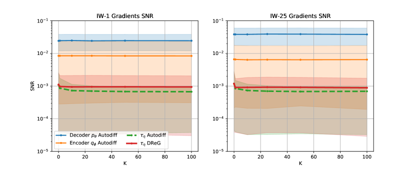
(a) IWHVI-VAE for $M=1$ and $M=25$

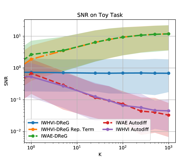
(b) Toy Task

Figure 3: Signal-to-Noise Ratio of gradients for different values of $K$. Solid lines denote SNR averaged over all model’s parameters, and shaded area marks 90% confidence interval over all parameters.

To evaluate the (D.1) gradient estimate we take a slightly trained (for 50 epochs by the usual gradient) VAE and compare signal-to-noise ratios of different gradients while varying $K$ and $M$. For each minibatch we recompute the vanilla autodiff gradients and a doubly reparametrized gradient (D.1) 100 times to estimate signal-to-noise ratio for each weight. We then average SNRs over different minibatches of fixed size, and present mean and 90% confidence intervals over different choices of weight in fig. 3(a).

We also compute SNR on a toy task from (Rainforth et al., 2018) for an upper bound (theorem A.1) on $\operatorname*{\mathbb{E}}_{q(x)}\log q(x)$ for ${q(x,z)=\mathcal{N}(x\mid z,I)\mathcal{N}(z\mid\theta,I)}$ and $\tau_{\eta}(z\mid x)=\mathcal{N}(z\mid Ax+b,2/3)$ for $\theta=[1,\dots,1],x,z\in\mathbb{R}^{10}$. We first train $\eta=\{A,b\}$ to optimality by making 1000 AMSGrad (Reddi et al., 2018) steps with learning rate $10^{-2}$ with batches of 100, then evaluate the gradients 1000 times with batches of size 100. We also include gradients of IWAE (coming from the task of lower bounding the $\operatorname*{\mathbb{E}}_{q(x)}\log q(x)$) to compare with. We compute SNR per parameter over these 1000 samples, and present results in fig. 3(b).

Best seen in the toy task, SNR of autodiff gradients decreases as $K$ grows, much resembling the standard IWAE issue, outlined by (Rainforth et al., 2018). IWHVI-DReG solves the problem, but only partially. While the SNR is no longer decreasing, it does not increase as in IWAE-DReG. While detailed study of this phenomena is outside the scope of this work, we show that it’s the second term (denoted $B$) in IWHVI-DReG, coming from the $\psi_{m0}$-based term in the bound, that causes the trouble. Indeed, if we omit this term, the (now biased) estimate would have higher SNR, essentially approaching the standard IWAE’s one. In practice, we found that the improved gradient estimate IWHVI-DReG significantly increased $D_{KL}(\tau(\psi\mid z)\mid\mid q(z))$, but this resulted in minor increases in the validation log-likelihood.

Appendix E Debiasing the bound

E.1 Deriving the bound

Following (Nowozin, 2018) we argue (lemma E.1) that

$$\mathcal{U}_{K}=\operatorname*{\mathbb{E}}_{p(\psi_{0}\mid z)}\operatorname*{\mathbb{E}}_{\tau(\psi_{1:K}\mid z)}\log\left(\frac{1}{K+1}\sum_{k=0}^{K}\frac{p(z,\psi_{k})}{\tau(\psi_{k}\mid z)}\right)=\log p(z)+\sum_{j=1}^{\infty}\frac{\gamma_{j}}{(K+1)^{j}}$$

So $\mathcal{U}_{K}$ can be seen as a biased estimator of marginal log-density $\log p(z)$ with bias of order $O(1/K)$. We can reduce this bias further by making use of the following fact:

$$(K+1)\mathcal{U}_{K}-K\mathcal{U}_{K-1} =\log p(z)-\frac{\gamma_{2}}{K(K+1)}+O\left(\tfrac{1}{K^{2}}\right)$$

$$=\log p(z)-\sum_{j=0}^{\infty}\frac{\gamma_{2}}{(K+1)^{j+2}}+O\left(\tfrac{1}{K^{2}}\right)$$

$$=\log p(z)-\frac{\gamma_{2}}{(K+1)^{2}}+O\left(\tfrac{1}{K^{2}}\right)$$

Averaging this identity over all possible choices of a subset of samples from $\tau(\psi\mid z)$ of size $K-1$, we obtain Jackknife-corrected estimator with bias of order $O(1/K^{2})$. One could then apply the same procedure again and again to obtain Generalized-order-$J$-Jackknife-corrected estimator with bias of order $O(1/K^{J+1})$, leading to a $J$-Jackknife upper marginal log-density estimate:

$$\mathcal{J}_{K}^{J}=\sum_{j=0}^{J}c(K,J,j)\overline{\mathcal{U}}_{K-j}$$ (10)

Where $\overline{\mathcal{U}}_{K-j}$ is $(K-j)$-samples bound averaged over all possible choices of a subset of size $K-j$ from $\psi_{1:K}$, and $c(K,J,j)$ are Sharot coefficients (Sharot, 1976; Nowozin, 2018):

$$\overline{\mathcal{U}}_{K-j}=\frac{1}{\binom{K}{K-j}}\sum_{S\subseteq\{1,\dots,K\}:|S|=K-j}\log\left(\frac{1}{K-j+1}\left[\frac{p(z,\psi_{0})}{\tau(\psi_{0}\mid z)}+\sum_{k\in S}\frac{p(z,\psi_{k})}{\tau(\psi_{k}\mid z)}\right]\right)$$

$$c(K,J,j)=(-1)^{j}\frac{(K-j)^{J}}{(J-j)!j!}$$

Despite not guaranteed to be an upper bound anymore, we still see that the estimate tends to overestimate the marginal log-density in practice.

Lemma E.1.

For fixed $p(\psi_{0}\mid z),\tau(\psi_{1:K}\mid z)$ and $z$ there exists a sequence $\{\gamma_{k}\}_{k=1}^{\infty}$ s.t.

$$\mathcal{U}_{K}=\log p(z)+\sum_{j=1}^{\infty}\frac{\gamma_{j}}{(K+1)^{j}}$$ (11)

Proof.

First, we note that $\mathcal{U}_{K}$ can be represented as marginal log-density plus some non-negative (due to theorem A.1) bias, which we’ll consider in greater detail.

$$\mathcal{U}_{K}=\operatorname*{\mathbb{E}}_{\begin{subarray}{c}p(\psi_{0}\mid z)\\ \tau(\psi_{1:K}\mid z)\end{subarray}}\log\left(\frac{1}{K+1}\sum_{k=0}^{K}\frac{p(z,\psi_{k})}{\tau(\psi_{k}\mid z)}\right)=\log p(z)+\overbrace{\operatorname*{\mathbb{E}}_{\begin{subarray}{c}p(\psi_{0}\mid z)\\ \tau(\psi_{1:K}\mid z)\end{subarray}}\log\left(\frac{1}{K+1}\sum_{k=0}^{K}\frac{p(\psi_{k}\mid z)}{\tau(\psi_{k}\mid z)}\right)}^{\text{Bias}}$$

Denote $w_{k}=\tfrac{p(\psi_{k}\mid z)}{\tau(\psi_{k}\mid z)}$, $w_{k}^{\prime}=w_{k}-1$ and expand the Bias around 1:

Bias $$=\sum_{n=1}^{\infty}\frac{(-1)^{n+1}}{n}\operatorname*{\mathbb{E}}_{p(\psi_{0}\mid z)}\operatorname*{\mathbb{E}}_{\tau(\psi_{1:K}\mid z)}\left(\tfrac{1}{K+1}\sum_{k=0}^{K}w_{k}^{\prime}\right)^{n}$$

$$=\sum_{n=1}^{\infty}\frac{(-1)^{n+1}}{n}\operatorname*{\mathbb{E}}_{p(\psi_{0}\mid z)}\operatorname*{\mathbb{E}}_{\tau(\psi_{1:K}\mid z)}\left(\tfrac{1}{K+1}w_{0}^{\prime}+\tfrac{K}{K+1}\overline{w_{1:K}^{\prime}}\right)^{n}$$

$$=\sum_{n=1}^{\infty}\frac{(-1)^{n+1}}{n}\sum_{m=0}^{n}{n\choose m}\operatorname*{\mathbb{E}}_{p(\psi_{0}\mid z)}\left(\tfrac{w_{0}^{\prime}}{K+1}\right)^{m}\operatorname*{\mathbb{E}}_{\tau(\psi_{1:K}\mid z)}\left(\tfrac{K}{K+1}\overline{w_{1:K}^{\prime}}\right)^{n-m}$$

$$=\sum_{n=1}^{\infty}\frac{(-1)^{n+1}}{n}\sum_{m=0}^{n}{n\choose m}\left(1-\tfrac{1}{K+1}\right)^{n-m}\left(\tfrac{1}{K+1}\right)^{n}\operatorname*{\mathbb{E}}_{p(\psi_{0}\mid z)}\left(w_{0}^{\prime}\right)^{m}\operatorname*{\mathbb{E}}_{\tau(\psi_{1:K}\mid z)}\left(\overline{w_{1:K}^{\prime}}\right)^{n-m}$$

Where $\overline{w_{1:K}^{\prime}}=\tfrac{1}{K}\sum_{k=1}^{K}w_{k}^{\prime}$ – an empirical average of zero-mean random variables. (A. Angelova, 2012) has shown that for a fixed $s\in\mathcal{N}$ there exist $\gamma_{1}^{(s)},\dots,\gamma_{T}^{(s)}$ s.t.

$$\operatorname*{\mathbb{E}}_{\tau(\psi_{1:K}\mid z)}\left(\overline{w_{1:K}^{\prime}}\right)^{s}=\sum_{t=1}^{T}\frac{\gamma_{t}^{(s)}}{K^{t}}=\sum_{t=1}^{T}\gamma_{t}^{(s)}\left[\sum_{n=1}^{\infty}\frac{1}{(K+1)^{n}}\right]^{t}$$

Therefore every addend in Bias depends on $K$ only through $1/(K+1)$, and thus decomposition (11) holds.

Note on convergence: while we have not shown the presented series to be convergent, in practice we only care about bias’ asymptotic behaviour up to an order of $1/(K+1)^{J}$, for which the decomposition works as long as the corresponding moments in Bias exist and are finite.

∎

E.2 Experiments

We only perform experimental validation of the Jackknife upper KL estimate (JHVI for short) in the same setting as in section 6.1. fig. 4 shows improved performance of the Jackknife-corrected estimate.

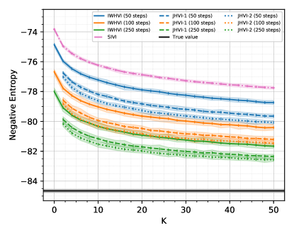
Figure 4: Negative entropy bound for 50-dimensional Laplace distribution. Shaded area denotes 90% confidence interval.

Appendix F Experiments Details

For MNIST we follow the setup by Mescheder et al. (2017): we use single 32-dimensional stochastic layer with ${p(z)}={\mathcal{N}(z\mid 0,I)}$ prior, decoder ${p_{\theta}(x\mid z)}={\text{Bernoulli}(x\mid\pi_{\theta}(z))}$ where $\pi_{\theta}$ is a neural network with two hidden 300-neurons layers and a softplus nonlinearity , and latent variable model encoder ${q_{\phi}(z\mid x)}=\int{\mathcal{N}(z\mid\mu_{\phi}(x,\psi),\sigma_{\phi}^{2}(x,\psi))}{\mathcal{N}(\psi\mid 0,1)}{d\psi}$ where ${\mu_{\phi}(x,\psi)}$ and ${\sigma_{\phi}^{2}(x,\psi)}$ are outputs of a neural network with architecture similar to as that of the decoder, except each next layer (including the one that generates distribution’s parameters) acts on previous layer’s output concatenated with input $\psi$. We take $\tau_{\vartheta}(\psi\mid z,x)=\mathcal{N}(\psi\mid\nu_{\vartheta}(x,z),\varsigma_{\vartheta}^{2}(x,z))$ where mean and variance are outputs of another neural network with same network architecture as that of the decoder, except it takes concatenation of $x$ and $z$ as input.

For OMNIGLOT we used simiar architecture, but for 50-dimensional $z$ and $\psi$, and all hidden layers had 200 neurons.

For flow-based models we used their implementations from TensorFlow Probability (Dillon et al., 2017). We had the encoder network output not only $\mu$ and $\sigma$, but also a context vector $h$ of same size as $z$ to be used to condition the flow transformations.

For IWHVI we used a grid search over 1) whether to use IWHVI-DReG (D.1), 2) whether to do inner KL (the $\log\tfrac{q(\psi)}{\tau(\psi\mid x,z)}$ terms) warm-up (linearly increase its weight from 0 to 1) for first 300 epochs, 3) whether to do outer KL warmup (the $\log\tfrac{p(z)}{\tfrac{1}{K+1}\sum\dots}$ term) for first 300 epochs, 4) Either use learning rate $\eta_{\text{base}}=10^{-3}$ with annealing $\eta=0.95^{\text{epoch}/100}\eta_{\text{base}}$ or $\eta=10^{-4}$ without annealing. We used the same grid for SIVI, except options (1) and (2) had no effect, since they only influenced $\tau$, and thus we did not serach over them. For HVM only the option (1) had no effect, since HVM does not sample from $\tau$.

In all experiments we did $10,000$ epochs with batches of size 256 and used Adam (Kingma and Ba, 2014) optimizer with $\beta_{1}=0.9,\beta_{2}=0.999$. We held out $5,000$ examples from trainsets to be used as validation.

References

-
A. Angelova (2012)
A. Angelova, J.
2012. On moments of sample mean and variance. International Journal of Pure and Applied Mathematics, 79. -
Agakov and Barber (2004)
Agakov, F. V. and D. Barber
2004. An auxiliary variational method. In International Conference on Neural Information Processing, Pp. 561–566. Springer. -
Atanov et al. (2019)
Atanov, A., A. Ashukha, K. Struminsky, D. Vetrov, and
M. Welling
2019. The deep weight prior. In International Conference on Learning Representations. -
Burda et al. (2015)
Burda, Y., R. Grosse, and R. Salakhutdinov
2015. Importance weighted autoencoders. arXiv preprint arXiv:1509.00519. -
Chen et al. (2016)
Chen, X., D. P. Kingma, T. Salimans, Y. Duan, P. Dhariwal, J. Schulman,
I. Sutskever, and P. Abbeel
2016. Variational lossy autoencoder. arXiv preprint arXiv:1611.02731. -
Dieng et al. (2017)
Dieng, A. B., D. Tran, R. Ranganath, J. Paisley, and
D. Blei
2017. Variational inference via upper bound minimization. In Advances in Neural Information Processing Systems, Pp. 2732–2741. -
Dillon et al. (2017)
Dillon, J. V., I. Langmore, D. Tran, E. Brevdo, S. Vasudevan, D. Moore,
B. Patton, A. Alemi, M. Hoffman, and R. A.
Saurous
2017. Tensorflow distributions. arXiv preprint arXiv:1711.10604. -
Dinh et al. (2016)
Dinh, L., J. Sohl-Dickstein, and S. Bengio
2016. Density estimation using real NVP. CoRR, abs/1605.08803. -
Domke and Sheldon (2018)
Domke, J. and D. R. Sheldon
2018. Importance weighting and variational inference. In Advances in Neural Information Processing Systems 31, S. Bengio, H. Wallach, H. Larochelle, K. Grauman, N. Cesa-Bianchi, and R. Garnett, eds., Pp. 4471–4480. Curran Associates, Inc. -
Goodfellow
et al. (2014)
Goodfellow, I., J. Pouget-Abadie, M. Mirza, B. Xu, D. Warde-Farley, S. Ozair,
A. Courville, and Y. Bengio
2014. Generative adversarial nets. In Advances in neural information processing systems, Pp. 2672–2680. -
Grosse et al. (2015)
Grosse, R. B., Z. Ghahramani, and R. P. Adams
2015. Sandwiching the marginal likelihood using bidirectional monte carlo. CoRR, abs/1511.02543. -
Guo et al. (2016)
Guo, F., X. Wang, K. Fan, T. Broderick, and D. B.
Dunson
2016. Boosting variational inference. arXiv preprint arXiv:1611.05559. -
Hinton and van
Camp (1993)
Hinton, G. E. and D. van Camp
1993. Keeping the neural networks simple by minimizing the description length of the weights. In Proceedings of the Sixth Annual Conference on Computational Learning Theory, COLT ’93, Pp. 5–13, New York, NY, USA. ACM. -
Huszár (2017)
Huszár, F.
2017. Variational inference using implicit distributions. arXiv preprint arXiv:1702.08235. -
Jebara and Pentland (2001)
Jebara, T. and A. Pentland
2001. On reversing jensen’s inequality. In Advances in Neural Information Processing Systems, Pp. 231–237. -
Kim et al. (2018)
Kim, Y., S. Wiseman, A. Miller, D. Sontag, and
A. Rush
2018. Semi-amortized variational autoencoders. In Proceedings of the 35th International Conference on Machine Learning, J. Dy and A. Krause, eds., volume 80 of Proceedings of Machine Learning Research, Pp. 2678–2687, Stockholmsmässan, Stockholm Sweden. PMLR. -
Kingma and
Ba (2014)
Kingma, D. P. and J. Ba
2014. Adam: A method for stochastic optimization. CoRR, abs/1412.6980. -
Kingma and Dhariwal (2018)
Kingma, D. P. and P. Dhariwal
2018. Glow: Generative flow with invertible 1x1 convolutions. In Advances in Neural Information Processing Systems 31, S. Bengio, H. Wallach, H. Larochelle, K. Grauman, N. Cesa-Bianchi, and R. Garnett, eds., Pp. 10235–10244. Curran Associates, Inc. -
Kingma et al. (2016)
Kingma, D. P., T. Salimans, R. Jozefowicz, X. Chen, I. Sutskever, and
M. Welling
2016. Improved variational inference with inverse autoregressive flow. In Advances in Neural Information Processing Systems 29, D. D. Lee, M. Sugiyama, U. V. Luxburg, I. Guyon, and R. Garnett, eds., Pp. 4743–4751. Curran Associates, Inc. -
Kingma and Welling (2013)
Kingma, D. P. and M. Welling
2013. Auto-encoding variational bayes. arXiv preprint arXiv:1312.6114. -
Kuleshov and Ermon (2017)
Kuleshov, V. and S. Ermon
2017. Neural variational inference and learning in undirected graphical models. In Advances in Neural Information Processing Systems, Pp. 6734–6743. -
Lake et al. (2015)
Lake, B. M., R. Salakhutdinov, and J. B.
Tenenbaum
2015. Human-level concept learning through probabilistic program induction. Science, 350(6266):1332–1338. -
LeCun et al. (1998)
LeCun, Y., L. Bottou, Y. Bengio, and P. Haffner
1998. Gradient-based learning applied to document recognition. Proceedings of the IEEE, 86(11):2278–2324. -
Louizos et al. (2017)
Louizos, C., K. Ullrich, and M. Welling
2017. Bayesian compression for deep learning. In Advances in Neural Information Processing Systems 30, I. Guyon, U. V. Luxburg, S. Bengio, H. Wallach, R. Fergus, S. Vishwanathan, and R. Garnett, eds., Pp. 3288–3298. Curran Associates, Inc. -
Maaløe et al. (2016)
Maaløe, L., C. K. Sønderby, S. K. Sønderby, and
O. Winther
2016. Auxiliary deep generative models. In Proceedings of The 33rd International Conference on Machine Learning, M. F. Balcan and K. Q. Weinberger, eds., volume 48 of Proceedings of Machine Learning Research, Pp. 1445–1453, New York, New York, USA. PMLR. -
MacKay (1995)
MacKay, D. J.
1995. Bayesian neural networks and density networks. Nuclear Instruments and Methods in Physics Research Section A: Accelerators, Spectrometers, Detectors and Associated Equipment, 354(1):73 – 80. Proceedings of the Third Workshop on Neutron Scattering Data Analysis. -
Mescheder et al. (2017)
Mescheder, L., S. Nowozin, and A. Geiger
2017. Adversarial variational bayes: Unifying variational autoencoders and generative adversarial networks. In International Conference on Machine Learning (ICML). -
Mohamed and
Lakshminarayanan (2016)
Mohamed, S. and B. Lakshminarayanan
2016. Learning in implicit generative models. arXiv preprint arXiv:1610.03483. -
Molchanov et al. (2018)
Molchanov, D., V. Kharitonov, A. Sobolev, and
D. Vetrov
2018. Doubly semi-implicit variational inference. arXiv preprint arXiv:1810.02789. -
Neal (2001)
Neal, R. M.
2001. Annealed importance sampling. Statistics and computing, 11(2):125–139. -