Analysis of Fully Discrete Mixed Finite Element Methods for Time-dependent Stochastic Stokes Equations with Multiplicative Noise

Abstract

This paper is concerned with fully discrete mixed finite element approximations of the time-dependent stochastic Stokes equations with multiplicative noise. A prototypical method, which comprises of the Euler-Maruyama scheme for time discretization and the Taylor-Hood mixed element for spatial discretization is studied in detail. Strong convergence with rates is established not only for the velocity approximation but also for the pressure approximation (in a time-averaged fashion). A stochastic inf-sup condition is established and used in a nonstandard way to obtain the error estimate for the pressure approximation in the time-averaged fashion. Numerical results are also provided to validate the theoretical results and to gauge the performance of the proposed fully discrete mixed finite methods.

1 Introduction

We consider the following time-dependent stochastic Stokes equations for viscous incompressible fluids:

(1a) $$du =\bigl{[}\nu\Delta u-\nabla p+f\bigr{]}dt+B(\cdot,u)dW(\cdot) \qquad\mbox{a.s. in}\,D_{T}:=(0,T)\times D,$$

(1b) $$\mbox{\rm div\,}u =0 \qquad\mbox{a.s. in}\,D_{T},$$

(1c) $$u =0 \qquad\mbox{a.s. on}\,\partial D_{T}:=(0,T)\times\partial D,$$

(1d) $$u(0) =u_{0} \qquad\mbox{a.s. in}\,D,$$

where $u$ and $p$ denote respectively the velocity field and the pressure of the fluid, and $f$ is a given source field. $D\subset\mathbf{R}^{d}(d=2,3)$ is a bounded domain with boundary $\partial D$, $B:[0,T]\times[H^{1}(D)]^{d}\to L_{0}(L^{2}(D),[L^{2}(D)]^{d})$ and $\{W(t);t\geq 0\}$ is an $[L^{2}(D)]^{d}$-valued $Q$-Wiener process (see Section 2 for their precise definitions).

The system of equations (1a), which is called stochastic Stokes equations/system, is a simplified version of the stochastic Navier-Stokes model for turbulent fluids (cf. [4, 3] and the references therein) by omitting the nonlinear term $-(u\cdot\nabla)u\,dt$ on the right-hand side of (1a). The stochastic term $B(\cdot,u)\,dW$, which often is called the noise, adds a solution-dependent source term to the corresponding deterministic Stokes (and the Navier-Stokes) system. When $B\equiv 0$, (1a) reduces to the time-dependent deterministic Stokes equations [30]. A motivation for adding such a noise term is to allow the stochastic models to capture the turbulence phenomenon with choosing a ”right” operator $B$ and a Wiener process $W$ by numerical simulation. Since the Stokes system (1a)–(1d) is a simplification of the more complicated stochastic Navier-Stokes system, all the results about mathematical theory established for the corresponding Navier-Stokes system clearly apply to the Stokes system. We refer the interested reader to [4, 3, 20, 21, 10] and the references therein for detailed discussions about solution concepts, well-posedness and regularity of solutions of the stochastic Navier-Stokes problems with various types of noises. We note that system (1) is nonlinear because $B(u)$ is a nonlinear function in $u$.

Since there exists a large amount of literature on numerical methods for the deterministic Stokes and Navier-Stokes equations, it is natural to try to adapt those successful numerical methods for solving problem (1). Indeed, with some special care on discretizing the stochastic term $B(\cdot,u)\,dW$, all other terms in (1a) can be discretized in the same way as done in the deterministic case. However, since in the stochastic case the solution $u$ is a Hilbert space-valued stochastic process and spatial norms of the velocity are only Hölder continuous in $t$, all the deterministic analysis techniques and machineries which require the differentiability of the solution in $t$ are not applicable in the stochastic case. Moreover, for saddle point problem (1), it is known [22] that the pressure process $\{p(t);0\leq t\leq T\}$ has very weak regularities (it is only a measure), which makes the numerical analysis of (1) quite challenging, especially for the mixed finite element discretization where the velocity and pressure are approximated simultaneously. As a result, the pool of rigorous numerical methods (i.e., those with support of convergence analysis) for the stochastic Stokes and Navier-Stokes equations is limited and those results only become available recently.

In [12] Carelli et al. proposed a Chorin-type time-splitting method for problem (1) to address the subtle interplay of noise and pressure. Strong convergence with rates was proved for the velocity approximation with sinusoidal noises. Although pressure approximation was also constructed and computed by the Chorin-type method, its convergence was not addressed in [12]. In addition, the semi-discrete in time Euler-Maruyama scheme was also considered and used as a tool in the analysis of the Chorin-type method, but its convergence analysis was not addressed. In [13] Carelli and Prohl proposed an implicit and a semi-implicit time discretizations for the stochastic Navier-Stokes problem in $2$-D with sinusoidal noises. Strong convergence with rates was also established for the velocity approximation. A fully discrete mixed finite element scheme was also considered and strong convergence with rates was also proved for the velocity approximation. As noted in [13], the interaction of Lagrange multipliers with the stochastic forcing in the scheme limits the accuracy of general discretely LBB-stable space discretizations. Strategies to overcome this difficulty were also proposed in [13] although the convergence of the pressure approximation was not addressed. Other recent works for stochastic Navier-Stokes equations include an iterative splitting scheme which was proposed in [6], a strong convergence in probability was established in the 2-D case for the velocity approximation. In a very recent paper [7], the authors proposed another time-splitting scheme and proved its strong $L^{2}$ convergence for the velocity approximation. In [31] a posterior error estimates were studied for a fully discrete divergence-free finite element method for the 2-D stochastic Navier-Stokes equations, both upper and lower a posterior error bounds were established for the velocity approximation in the paper. The paper [9] by Brzeźniak, et al., which perhaps is closest to this paper, proposed two time-stepping schemes for mixed finite element spatial discretizations of the stochastic Navier-Stokes equations with general multiplicative noise and established the convergence for the velocity approximation (as a function sequence) to weak martingale solutions in 3-D and to strong solutions in 2-D using the compactness argument. Since the analysis was done in the space of discretely solenoidal functions which allows to eliminate the discrete pressures from the schemes, consequently, the convergence of the pressure approximations was bypassed in [9]; in addition, no rate of convergence was presented for the velocity approximation. To the best of our knowledge, no convergence (hence, no rate of convergence) for a pressure approximation has been reported in the literature for system (1).

The primary goal of this paper is to analyze convergence behaviors of the mixed finite element method for the stochastic Stokes problem (1) with general multiplicative noise. Specifically, we shall establish strong convergence with rates not only for the velocity approximation but also for the pressure approximation (in a time-averaged fashion). A secondary goal of the paper is to use (1) as a prototypical example to develop numerical analysis techniques which can be useful for analyzing mixed finite element approximations of the stochastic Navier-Stokes equations and possibly other nonlinear stochastic PDEs.

The remainder of this paper is organized as follows. In Section 2 we introduce function and space notation and some background materials for problem (1) and establish a few preliminary results such as the stochastic inf-sup condition and Hölder continuity in time of the solution in various spatial norms. These results plays an important role in the error analysis of this paper. In Section 3 we state the Euler-Maruyama time-stepping scheme for problem (1) and derive some error estimates for both the velocity and pressure approximations. In Section 4 we formulate a fully discrete mixed finite element method which uses the prototypical Taylor-Hood mixed finite element method for spatial discretization. The highlight of this Section is to establish the following error estimates for the numerical solution $(u_{h}^{n},p_{h}^{n})$:

(2) $$\max_{1\leq n\leq N}\Bigl{(}E\Bigl{[}\|u(t_{n})-u^{n}_{h}\|^{2}_{L^{2}}\Bigl{]}\Bigl{)}^{\frac{1}{2}} +\Bigl{(}E\Bigl{[}k\sum_{n=1}^{N}\|\nabla(u(t_{n})-u^{n}_{h})\|^{2}_{L^{2}}\Bigr{]}\Bigr{)}^{\frac{1}{2}}$$

$$\leq\hat{C}_{1}k^{\frac{1}{2}}+\hat{C}_{2}k^{-\frac{1}{2}}h,$$

(3) $$\max_{1\leq n\leq N}\Bigl{(}E\Bigl{[}\|\nabla(u(t_{n})-u^{n}_{h})\|^{2}_{L^{2}}\Bigr{]}\Bigr{)}^{\frac{1}{2}} +\Bigl{(}E\Bigl{[}k\sum_{n=1}^{N}\|A(u(t_{n})-u^{n}_{h})\|^{2}_{L^{2}}\Bigr{]}\Bigr{)}^{\frac{1}{2}}$$

$$\leq\hat{C}_{3}k^{\frac{1}{2}}+\hat{C}_{4}k^{-\frac{1}{2}}h,$$

(4) $$\max_{1\leq n\leq N}\Bigl{(}E\Bigl{[}\|A(u(t_{n})-u^{n}_{h})\|^{2}_{L^{2}}\Bigr{]}\Bigr{)}^{\frac{1}{2}} +\Bigl{(}E\Bigl{[}k\sum_{n=1}^{N}\|A^{\frac{3}{2}}(u(t_{n})-u^{n}_{h})\|^{2}_{L^{2}}\Bigr{]}\Bigr{)}^{\frac{1}{2}}$$

$$\leq\hat{C}_{5}k^{\frac{1}{2}}+\hat{C}_{6}k^{-\frac{1}{2}}h,$$

(5) $$\max_{1\leq m\leq N}E\Bigl{[}\Bigl{\|}\int_{0}^{t_{m}}p(s)ds-k\sum^{m}_{n=1}p^{n}_{h}\Bigr{\|}_{L^{2}}\Bigr{]} \leq\hat{C}_{7}k^{\frac{1}{2}}+\hat{C}_{8}k^{-\frac{1}{2}}h.$$

It should be noted that the (bad) $k^{-\frac{1}{2}}$ factor in the above error estimates is due to the low regularity of the pressure $p$ and the simultaneous approximation property of the mixed method. Obviously, compared to the error estimates for mixed finite element approximations of the deterministic Stokes problem (cf. [24]), the above estimates seem inferior, however, our numerical experiments indicate that these estimates are in fact sharp for the stochastic Stokes problem (1). The above theoretical results on one hand reveal the insight of the (damaging) effect of the noise on the performance of the standard mixed finite element method for the stochastic Stokes problem and on the other hand suggest that modifications and improvements must be done to the standard mixed finite element method in order to improve its performance so that the modified method (such as mixed-primal finite element method, stabilized finite element method) could produce competitive velocity approximations with that of divergence-free finite element methods (cf. [13]). Finally, in Section 5, we provide some numerical experiments to validate our theoretical results and to gauge the performance of the proposed numerical method.

2 Preliminaries

2.1 Notation and assumptions

Standard function and space notation will be adopted in this paper. In particular, for a given positive integer $m$, let $H^{m}(D)$ denote the standard Sobolev space consisting of all real-valued functions whose up to $m$th order weak derivatives are $L^{2}$-integrable on $D\subset\mathbf{R}^{d}$, and $\|\cdot\|_{H^{m}}$ denotes its norm. Let $H^{1}_{0}(D)$ be the subspace of $H^{1}(D)$ whose functions have zero trace on $\partial D$, $H^{0}(D):=L^{2}(D)$ and $(\cdot,\cdot):=(\cdot,\cdot)_{D}$ denote the standard $L^{2}$-inner product. Let $(\Omega,\mathcal{F},\mathcal{F}_{t},\mathbb{P})$ be a probability space with $\sigma$-algebra $\mathcal{F}$, the normal filtration $\mathcal{F}_{t}$ and the probability measure $\mathbb{P}$. For a random variable $v$ defined on $(\Omega,\mathcal{F},\mathcal{F}_{t},\mathbb{P})$, let $E[v]$ denote the expected value of $v$. We also let $(\Omega,\mathcal{F},\{\mathcal{F}_{t}\},\mathbb{P})$ be a complete probability space with continuous filtration $\{\mathcal{F}_{t}\subset\mathcal{F};t\geq 0\}$. a.s. means almost surely with respect to the probability measure $\mathbb{P}$. For a Banach space $Y$, let $L^{p}(0,T;Y)$ denote the time-space function space endowed with following norm:

$$\|w\|_{L^{p}(0,T;Y)}:=\left\{\begin{array}[]{ll}\bigl{(}\int_{0}^{T}\|w\|_{Y}^{p}dt\bigr{)}^{\frac{1}{p}}&\,\mbox{if}\,\,\,\,1\leq p<\infty,\\ \\ \underset{t\in[0,T]}{\mbox{\rm ess sup }}\|w\|_{Y}&\,\mbox{if}\,\,\,\,p=\infty.\end{array}\right.$$

We shall often use the abbreviated notation $L^{p}(Y):=L^{p}(0,T;Y)$ for convenience.

For a normed vector space $X$ with norm $\|\cdot\|_{X}$, let $[X]^{d}$ denote the space of all $d$-vector-valued mappings whose components belong to $X$. Define the Bochner space

$$L^{p}(\Omega,X):=\bigl{\{}v:\Omega\rightarrow X;\,E[\|v\|_{X}^{p}]<\infty\bigr{\}}$$

and the norm

$$\|v\|_{L^{p}(\Omega,X)}:=\Bigl{(}E\Bigl{[}\|v\|_{X}^{p}\Bigr{]}\Bigr{)}^{\frac{1}{p}},\qquad 1<p<\infty.$$

We also introduce the following special space notation:

$$\mathcal{V}:=[H^{1}_{0}(D)]^{d},\mathcal{V}_{*}:=[H^{2}_{0}(D)]^{d},\quad\mathcal{W}=L^{2}_{0}(D):=\{v\in L^{2}(D);\,(v,1)_{D}=0\},$$

$$\mathcal{V}_{0}:=\bigl{\{}v\in\mathcal{V};\,\mbox{\rm div\,}v=0\mbox{ in }D\bigr{\}},\quad\mathbb{V}:=L^{2}(\Omega,\mathcal{V}),\quad\mathbb{W}:=L^{2}(\Omega,\mathcal{W}).$$

To give a meaning to the stochastic term $B(\cdot,u)\,dW$, we need to recall the definition of Hilbert space-valued $Q$-Wiener process $W$. Let $Q$ be a non-negative and symmetric linear operator from $L^{2}(D)$ to itself. Assume that $Q$ has a set of eigenvalues and eigenfunctions $\{(\lambda_{j},q_{j})\}_{j\geq 1}$ such that $\{q_{j}\}_{j\geq 1}$ forms an orthonormal basis for $L^{2}(D)$. Let $\{\beta_{j}(t);t\geq 0\}_{j\geq 1}$ be a sequence of independent identically distributed (iid) real-valued Brownian motions (or Wiener processes) adapted to $\{\mathcal{F}_{t}\}$. Then an $L^{2}(D)$-valued $Q$-Wiener process $W=\{W(t);t\geq 0\}$ on $(\Omega,\mathcal{F},\{\mathcal{F}_{t}\},\mathbb{P})$ is defined as

(6) $$W(\cdot,t)=\sum_{j=1}^{\infty}\sqrt{\lambda_{j}}q_{j}(\cdot)\beta_{j}(t)\qquad\mbox{a.s. in }D.$$

Let $\mathcal{K}_{*}:=Q^{\frac{1}{2}}(L^{2}(D))$ be the Cameron-Martin space for the Wiener measure on $C([0,T];L^{2}(D))$ equipped with the scalar product $(\varphi,\psi)_{\mathcal{K}_{*}}=(Q^{-\frac{1}{2}}\varphi,Q^{-\frac{1}{2}}\psi)_{L^{2}(D)}$ for all $\varphi,\psi\in L^{2}(D)$, where $Q^{-\frac{1}{2}}$ denotes the pseudoinverse of $Q^{\frac{1}{2}}$. Let $\mathcal{K}:=L_{0}(L^{2}(D);[L^{2}(D)]^{d})$ be the Banach space of linear operators from $L^{2}(D)$ to $[L^{2}(D)]^{d}$ which have finite Hilbert-Schmidt norms denoted by $\|\cdot\|_{\mathcal{K}}$. For any $1<p<\infty$, let $M^{p}_{\mathcal{F}_{t}}(\Omega,L^{p}(0,T;\mathcal{K}))$ be the subspace of the Bochner space $L^{p}(\Omega,L^{p}(0,T;\mathcal{K}))$ whose mappings are $\{\mathcal{F}_{t}\}$-adapted. Then for any $\varphi\in M^{2}_{\mathcal{F}_{t}}(\Omega,L^{2}(0,T;\mathcal{K}))$, the stochastic integral $\int_{0}^{t}\varphi(s)\,dW(s)$ for $0\leq t\leq T$ is defined as an $[L^{2}(D)]^{d}$-valued function by

(7) $$\Bigl{(}\int_{0}^{t}\varphi(s)\,dW(s),\chi\Bigr{)}=\lim_{J\rightarrow\infty}\sum^{J}_{j=1}\sqrt{\lambda_{j}}\int_{0}^{t}\bigl{(}\varphi(s)q_{j},\chi\bigr{)}\,d\beta_{j}(s)\quad\forall\chi\in[L^{2}(D)]^{d},\,a.s.$$

Note that the stochastic integral on the right-hand side is understood in the Itô’s sense. It is well-known [28] that $\int_{0}^{t}\varphi(s)dW(s)$ is an $\{\mathcal{F}_{t}\}$-martingale and there holds the following Itô’s isometry:

(8) $$E\Bigl{[}\Bigl{\|}\int_{0}^{T}\varphi(s)\,dW(s)\Bigr{\|}_{L^{2}(D)}^{2}\Bigr{]}=E\Bigl{[}\int_{0}^{T}\|\varphi(s)\|^{2}_{\mathcal{K}}\,ds\Bigr{]}.$$

The above definition of stochastic integrals suggests that $B(\cdot,u)$ needs to belong to $M^{2}_{\mathcal{F}_{t}}(\Omega,L^{2}(0,T;\mathcal{K}))$ in order to give a meaning to the stochastic term in (1a). Indeed, in this paper we assume that $B:[0,T]\times[L^{2}(D)]^{d}\rightarrow L^{2}(\Omega,\mathcal{K})$ is Hölder-Lipschitz continuous in time and has a linear growth in the second argument in the sense that there exists a constant $C_{T}>0$ such that $\mathbb{P}$-a.s.

(9a) $$\|D^{j}(B(s,v)-B(t,w))\|_{\mathcal{K}} \leq C_{T}\bigl{[}|s-t|^{\frac{1}{2}}+\|D^{j}(v-w)\|_{L^{2}}\bigr{]},\quad j=0,1,2,$$

(9b) $$|D^{i}B(t,v)| \leq C_{T}\bigl{(}1+\|D^{i}v\|_{L^{2}}\bigr{)},\ \ \ i=0,1,2,3,4$$

for any $v,w\in[L^{2}(D)]^{d},\,s,t\in[0,T]$, for $v\in[L^{2}(D)]^{d}$.

(10) $$B(\cdot,v)\in L^{2}(\Omega;L^{2}(0,T;\mathcal{K})).$$

Finally, we assume that $D\subset\mathbf{R}^{d}(d=2,3)$ is a bounded domain such that there is a unique strong solution $(v,\chi)\in\mathcal{V}_{0}\cap[H^{2}(D)]^{d}\times L^{2}_{0}(D)\cap H^{1}(D)$ to the following deterministic stationary Stokes problem:

$$-\nu\Delta v+\nabla\chi =g \qquad\mbox{in }D,$$

$$\mbox{\rm div\,}v =0 \qquad\mbox{in }D,$$

$$v =0 \qquad\mbox{on }\partial D,$$

which satisfies the estimate

$$\|v\|_{H^{2}(D)}+\|\chi\|_{H^{1}(D)}\leq C\|g\|_{L^{2}(D)}$$

for any $g\in L^{2}(D)$. It is well-known [30] that the above regularity holds if $D$ is a convex polygonal domain in 2-D, while in $3$-D it holds for $C^{2}$-domains.

2.2 Properties of variational weak solutions

In this subsection we first recall the variational weak solution definition for problem (1). We then prove a stochastic inf-sup condition for the mixed term and establish some Hölder continuity (in time) of various spatial norms of weak solutions. These auxiliary results will play an important role in our convergence analysis to be given in the subsequent sections.

Definition 1.

([22]) Suppose that $u_{0}\in L^{2}(\Omega,\mathcal{V}_{0})$ and $f\in L^{2}(\Omega,L^{\infty}(0,T;$ $[L^{2}(D)]^{d})$. A pair of $\{\mathcal{F}_{t}\}$-adapted stochastic processes $\{(u(t),p(t));0\leq t\leq T\}$ is called a weak solution of (1) if $(u,p)\in L^{2}\bigl{(}\Omega,L^{\infty}(0,T;[L^{2}(D)]^{d})\cap L^{2}(0,T;\mathcal{V})\cap C(0,T;\mathcal{V}^{*})\bigr{)}\times L^{2}\bigl{(}\Omega,L^{2}(0,T;W^{-1,\infty}(D))\bigr{)}$ and satisfy $\mathbb{P}$-a.s

(11a) $$\bigl{(}u(t),\psi\bigr{)}+\int_{0}^{t}\nu a(u(s),\psi)\,ds+b\Bigl{(}\psi,\int_{0}^{t}p(s)\,ds\Bigr{)}$$

$$\qquad=(u_{0},\psi)+\int_{0}^{t}\bigl{(}f(s),\psi\bigr{)}\,ds+\Bigl{(}\int_{0}^{t}B(s,u(s))\,dW(s),\psi\Bigr{)} \qquad\forall\psi\in\mathcal{V},$$

(11b) $$b(u,q)=0\qquad\forall q\in\mathcal{W}$$

for all $t\in(0,T]$. Where the bilinear forms $a(\cdot,\cdot)$ and $b(\cdot,\cdot)$ are defined as follows:

(12a) $$a(v,w) :=\bigl{(}\nabla v,\nabla w\bigr{)} \qquad\forall v,w\in\mathcal{V},$$

(12b) $$b(v,q) :=\bigl{(}\mbox{\rm div\,}v,q\bigr{)} \qquad\forall v\in\mathcal{V},\,q\in\mathcal{W}.$$

Remark 1.

We write $b\Bigl{(}\psi,\int_{0}^{t}p(s)\,ds\Bigr{)}$ instead of $\int_{0}^{t}b(\psi,p(s))\,ds$ in (11a) because the regularity of $p$ is too weak to allow the latter to make sense unless more smoother test function $\psi$ is used. On the other hand, it could be shown that $\int_{0}^{t}p(s)\,ds\in L^{2}\bigl{(}\Omega,L^{2}(D\times(0,T))\bigr{)}$ so the former is well defined. Thus, in the remainder of this paper, the pressure process $\{p(t)\}_{t\geq 0}$ will always appear in the time integral form.

It should also be noted that other solution notions such as mild and strong solutions have also be introduced and studied in the literature for problem (1) (cf. [28, 14] and the references therein). In addition, nonhomogeneous boundary conditions can be dealt with through standard lifting arguments. In this paper, we only consider homogeneous boundary conditions to avoid the technicalities.

Next, we state a stochastic inf-sup condition for the bilinear form $b(\cdot,\cdot)$.

Lemma 2.

There exists a positive constant $\beta$ such that

(13) $$\sup_{v\in\mathbb{V}}\frac{E[b(v,q)]}{\|v\|_{\mathbb{V}}}\geq\beta\|q\|_{\mathbb{W}}\qquad\forall q\in\mathbb{W}.$$

Proof.

Below we give a proof for the sake of completeness. The proof follows the same lines as that for the deterministic inf-sup condition (cf. [2, 24]), we only sketch the main ideas and steps of the proof in the case when $D$ is a 2-D bounded domain with smooth or convex polygonal boundary $\partial D$.

For any fixed $q\in\mathbb{W}$, the first step of the proof is to construct a random field $v_{1}\in L^{2}(\Omega,[H^{1}(D)]^{d})$ such that $\mbox{\rm div\,}v_{1}=q$ in $L^{2}(\Omega\times D)$ and $v_{1}\cdot n=0$ a.s. on $\partial D$, where $n$ denotes the unit outward normal to $\partial D$. In addition, there exists a positive constant $c_{1}$ such that

(14) $$\|v_{1}\|_{L^{2}(\Omega,[H^{1}(D)]^{d})}\leq c_{1}\|q\|_{\mathbb{W}}.$$

The desired random field $v_{1}$ can be chosen as $v_{1}=-\nabla\phi$, where $\phi\in L^{2}(\Omega,H^{2}(D))$ is the solution of the following random Poisson problem:

$$-\Delta\phi =q\qquad\mbox{a.s. in }D,$$

$$\frac{\partial\phi}{\partial n} =0\qquad\mbox{a.s. on }\partial D,$$

$$(\phi,1) =0\qquad\mbox{a.s.}$$

By the elliptic PDE theory we know that there exists a unique solution $\phi$, moreover, there exists a positive constant $c_{1}$ such that

$$\|\phi\|_{H^{2}(D)}\leq c_{1}\|q\|_{L^{2}(D)}\qquad\mbox{a.s.}$$

which clearly implies (14) with $v_{1}=-\nabla\phi$.

The second step of the proof is to construct a random field $v_{2}\in L^{2}(\Omega,[H^{1}(D)]^{d})$ such that $\mbox{\rm div\,}v_{2}=0$ in $L^{2}(\Omega\times D)$, $v_{2}\cdot\tau=-v_{1}\cdot\tau$ and $v_{2}\cdot n=0$ a.s. on $\partial D$, where $\tau$ denotes the positively oriented unit tangent vector to $\partial D$. In addition, there exists a positive constant $c_{2}$ such that

(15) $$\|v_{2}\|_{L^{2}(\Omega,[H^{1}(D)]^{d})}\leq c_{2}\|v_{1}\|_{L^{2}(\Omega,[H^{1}(D)]^{d})}.$$

One such a random field is $v_{2}=\mbox{\rm curl\,}\psi$, where $\psi\in L^{2}(\Omega,H^{2}(D))$ satisfies

$$\Delta^{2}\psi =0 \qquad\mbox{a.s. in }D,$$

$$\frac{\partial\psi}{\partial n} =v_{1}\cdot\tau \qquad\mbox{a.s. on }\partial D,$$

$$\psi =0 \qquad\mbox{a.s. on }\partial D,$$

and

$$\|\psi\|_{H^{2}(D)}\leq c_{2}\|v_{1}\|_{H^{1}(D)}\qquad\mbox{a.s.}$$

for some positive constant $c_{2}$. Note that the existence of $\psi$ is guaranteed by the elliptic PDE theorey. The above estimate immediately infers (15).

The third step of the proof is to define $z=v_{1}+v_{2}$. It is easy to check that $z\in L^{2}(\Omega,[H^{1}(D)]^{d})$, $\mbox{\rm div\,}z=q$ in $L^{2}(\Omega\times D)$ and $z=0$ a.s. on $\partial D$, hence, $z\in\mathbb{V}$. Moreover, it follows from (14) and (15) and the triangle inequality that

(16) $$\|z\|_{\mathbb{V}}\leq(1+c_{2})\|v_{1}\|_{L^{2}(\Omega,[H^{1}(D)]^{d})}\leq(1+c_{2})c_{1}\|q\|_{\mathbb{W}}.$$

Finally, it follows from (16) that

$$\sup_{v\in\mathbb{V}}\frac{E[b(v,q)]}{\|v\|_{\mathbb{V}}}\geq\frac{E[b(z,q)]}{\|z\|_{\mathbb{V}}}=\frac{E\bigl{[}\|q\|_{L^{2}(D)}^{2}\bigr{]}}{\|z\|_{\mathbb{V}}}\geq\frac{1}{(1+c_{2})c_{1}}\|q\|_{\mathbb{W}}.$$

Hence, (13) holds with $\beta=\frac{1}{(1+c_{2})c_{1}}$. The proof is complete. ∎

The next theorem establishes some Hölder continuity (in time) of the velocity field $u$ in various spatial norms.

Theorem 3.

Let $(u,p)$ be the weak solution to problem (1), and assume that $u\in L^{2}(\Omega,L^{\infty}(0,T;\mathcal{V}\cap[H^{3}(D)]^{d})),\nabla u_{j},Au,A^{\frac{3}{2}}u\in L^{2}(\Omega;C([0,T];[L^{2}(D)]^{d}))$ for $1\leq j\leq d$, and $f\in L^{2}(\Omega;L^{\infty}(0,T,H^{1}(D)^{d}))$. Then there hold

(17a) $$E\bigl{[}\|u(t)-u(s)\|^{2}_{L^{2}}\bigr{]}+\nu E\Bigl{[}\int_{s}^{t}\|\nabla(u(\xi)-u(s))\|_{L^{2}}^{2}\Bigr{]}d\xi\leq C_{1}|t-s|,$$

(17b) $$E\bigl{[}\|\nabla(u(t)-u(s))\|^{2}_{L^{2}}\bigr{]}+\nu E\Bigl{[}\int_{s}^{t}\|A(u(\xi)-u(s))\|_{L^{2}}^{2}\Bigr{]}d\xi\leq C_{2}|t-s|,$$

(17c) $$E\bigl{[}\|A(u(t)-u(s))\|^{2}_{L^{2}}\bigr{]}+\nu E\Bigl{[}\int_{s}^{t}\|A^{\frac{3}{2}}(u(\xi)-u(s))\|_{L^{2}}^{2}\Bigr{]}d\xi\leq C_{3}|t-s|$$

for any $0\leq s,t\leq T$, where

$$C_{1}=\Bigl{(}(2\nu+2C_{0}C_{T})E[\|\nabla u\|_{L^{\infty}(L^{2})}^{2}]+\frac{2}{\nu}E[\|f\|^{2}_{L^{\infty}(H^{-1})}]\Bigr{)}(1+2C_{T}T)e^{2C_{T}T},$$

$$C_{2}=\Bigl{(}(2\nu+2C_{0}C_{T})E\bigl{[}\|Au\|_{L^{\infty}(L^{2})}^{2}\bigr{]}+\frac{2}{\nu}E\bigl{[}\|f\|^{2}_{L^{\infty}(L^{2})}\bigr{]}\Bigr{)}(1+2C_{T}T)e^{2C_{T}T},$$

$$C_{3}=\Bigl{(}(2\nu+2C_{0}C_{T})E\bigl{[}\|A^{\frac{3}{2}}u\|_{L^{\infty}(L^{2})}^{2}\bigr{]}+\frac{2}{\nu}E\bigl{[}\|f\|^{2}_{L^{\infty}(H^{1})}\bigr{]}\Bigr{)}(1+2C_{T}T)e^{2C_{T}T},$$

where $A:\mathcal{V}\cap[H^{2}(D)]^{d}\to\mathcal{V}_{0}$ denotes the Stokes operator (cf. [30]) and $C_{0}$ is the constant in the Poincaré inequality for $H^{1}(D)$ functions.

Proof.

We first note that estimate (17a) was obtained in [9, 13] using the semigroup approach, the results of (17b)–(17c) seem new. Below we give a proof for each estimate using the Itô’s formula approach.

Step 1: For a fix $s\in(0,T]$, by the definition of weak solutions we obtain

$$\bigl{(}u(t)-u(s),v\bigr{)}+\nu\int_{s}^{t}a(u,v)\,d\xi=\int_{s}^{t}(f,v)\,d\xi+\Bigl{(}\int_{s}^{t}B(\xi,u)\,dW(\xi),v\Bigr{)}$$

for any $v\in\mathcal{V}_{0}$. Now apply Itô’s formula to $\Phi(u(t)):=\|u(t)-u(s)\|^{2}_{L^{2}}$ to get

(18) $$\|u(t)-u(s)\|^{2}_{L^{2}}+2\nu\int_{s}^{t}\bigl{(}\nabla u(\xi),\nabla(u(\xi)-u(s))\bigr{)}\,d\xi$$

$$\qquad=2\int_{s}^{t}\bigl{(}f(\xi),u(\xi)-u(s)\bigr{)}\,d\xi+2\int_{s}^{t}\Bigl{(}B(\xi,u(\xi))\,dW(\xi),u(\xi)-u(s)\Bigr{)}$$

$$\qquad\qquad+\int_{s}^{t}\|B(\xi,u(\xi))\|^{2}_{\mathcal{K}}\,d\xi.$$

Then we have

(19) $$\|u(t)-u(s)\|^{2}_{L^{2}}+2\nu\int_{s}^{t}\|\nabla u(\xi)-u(s)\bigr{|}_{L^{2}}^{2}\,d\xi$$

$$\qquad=2\nu\int_{s}^{t}\bigl{(}\nabla u(s),\nabla(u(\xi)-u(s))\bigr{)}\,d\xi+2\int_{s}^{t}\bigl{(}f(\xi),u(\xi)-u(s)\bigr{)}\,d\xi$$

$$\qquad\qquad+\int_{s}^{t}\|B(\xi,u(\xi))\|^{2}_{\mathcal{K}}\,d\xi+2\int_{s}^{t}\Bigl{(}B(\xi,u(\xi))\,dW(\xi),u(\xi)-u(s)\Bigr{)}$$

$$\qquad=:I_{1}+I_{2}+I_{3}+I_{4}.$$

We then bound each $I_{i}$ for $i=1,2,3,4$ separately below.

To bound $I_{1}$, by Schwarz and Young’s inequality we get

(20) $$2\nu\int_{s}^{t}\bigl{(}\nabla u(s), \nabla(u(\xi)-u(s))\bigr{)}\,d\xi\leq 2\nu\int_{s}^{t}\|\nabla u(s)\|_{L^{2}}\|\nabla(u(\xi)-u(s)))\|_{L^{2}}\,d\xi$$

$$\leq 2\nu\Bigl{(}\int_{s}^{t}\|\nabla(u(\xi)-u(s))\|_{L^{2}}^{2}\,d\xi\Bigr{)}^{\frac{1}{2}}\Bigl{(}\int_{s}^{t}\|\nabla u(s)\|_{L^{2}}^{2}\,d\xi\Bigr{)}^{\frac{1}{2}}$$

$$\leq\frac{\nu}{2}\int_{s}^{t}\|\nabla(u(\xi)-u(s))\|^{2}_{L^{2}}\,d\xi+2\nu\|\nabla u(s)\|_{L^{2}}^{2}\,|t-s|.$$

Similarly, $I_{2}$ can be bounded as follows:

(21) $$2\int_{s}^{t}\bigl{(}f(\xi), u(\xi)-u(s)\bigr{)}\,d\xi\leq 2\Bigl{(}\varepsilon\int_{s}^{t}\|\nabla(u(\xi)-u(s))\|_{L^{2}}^{2}\,d\xi$$

$$\hskip 86.72377pt+\frac{1}{4\varepsilon}\int_{s}^{t}\|f(\xi)\|_{H^{-1}}^{2}\,d\xi\Bigr{)}$$

$$\leq 2\Bigl{(}\varepsilon\int_{s}^{t}\|\nabla(u(\xi)-u(s))\|_{L^{2}}^{2}\,d\xi+\frac{1}{4\varepsilon}\int_{s}^{t}\|f(\xi)\|_{H^{-1}}^{2}\,d\xi\Bigr{)}$$

$$\leq\frac{\nu}{2}\int_{s}^{t}\|\nabla(u(\xi)-u(s))\|_{L^{2}}^{2}\,d\xi+\frac{2}{\nu}\|f\|^{2}_{L^{\infty}(H^{-1})}\,|t-s|,$$

where we set $\varepsilon=\frac{\nu}{4}$.

To bound $I_{3}$, we have

(22) $$\int_{s}^{t}\|B(\xi,u(\xi))\|^{2}_{\mathcal{K}}\,d\xi=\int_{s}^{t}\|B(\xi,u(\xi))-B(s,u(s))+B(s,u(s))\|^{2}_{\mathcal{K}}\,d\xi$$

$$\qquad\leq 2\int_{s}^{t}\|B(\xi,u(\xi))-B(s,u(s))\|^{2}_{\mathcal{K}}\,d\xi+2\int_{s}^{t}\|B(s,u(s))\|^{2}_{\mathcal{K}}\,d\xi$$

$$\qquad\leq 2C_{T}\int_{s}^{t}\|u(\xi)-u(s)\|^{2}_{L^{2}}\,d\xi+2C_{T}\int_{s}^{t}\|u(s)\|^{2}_{L^{2}}\,d\xi$$

$$\qquad\leq 2C_{T}\int_{s}^{t}\|u(\xi)-u(s)\|^{2}_{L^{2}}\,d\xi+2C_{T}\|u(s)\|^{2}_{L^{2}}\,|t-s|.$$

Finally, on noticing that $I_{4}$ is a martingale, then we have $E[I_{4}]=0$. Now combining (20)–(22) and taking the expectation we obtain

$$E\bigl{[}\|u(t)-u(s)\|^{2}_{L^{2}}\bigr{]}+\nu E\Bigl{[}\int_{s}^{t}\|\nabla(u(\xi)-u(s))\|_{L^{2}}^{2}\,d\xi\Bigr{]}$$

$$\qquad\leq\Bigl{(}2\nu E\bigl{[}\|\nabla u(s)\|_{L^{2}}^{2}\bigr{]}+2C_{T}E\bigl{[}\|u(s)\|_{L^{2}}^{2}\bigr{]}+\frac{2}{\nu}E\bigl{[}\|f\|^{2}_{L^{\infty}(H^{-1})}\bigr{]}\Bigr{)}\,|t-s|$$

$$\qquad\qquad+2C_{T}E\Bigl{[}\int_{s}^{t}\|u(\xi)-u(s)\|^{2}_{L^{2}}\,d\xi\Bigr{]}.$$

An application of Gronwall and Poincaré inequality yields

$$E\bigl{[}\|u(t)-u(s)\|^{2}_{L^{2}}\bigr{]}+\nu E\Bigl{[}\int_{s}^{t}\|\nabla(u(\xi)-u(s))\|_{L^{2}}^{2}\,d\xi\Bigr{]}$$

$$\,\,\leq\Bigl{(}(2\nu+2C_{0}C_{T})E[\|\nabla u\|_{L^{\infty}(L^{2})}^{2}]+\frac{2}{\nu}E[\|f\|^{2}_{L^{\infty}(H^{-1})}]\Bigr{)}(1+2C_{T}T)e^{2C_{T}T}\,|t-s|.$$

Hence, (17a) holds.

Step 2: To show the second inequality (17b), we apply Itô’s formula to $\Psi(u(t)):=\|\nabla(u(t)-u(s))\|^{2}_{L^{2}}$ to get

(23) $$\|\nabla(u(t)-u(s))\|^{2}_{L^{2}}+2\nu\int_{s}^{t}\bigl{(}Au(\xi)-u(s),A(u(\xi)-u(s))\bigr{)}\,d\xi$$

$$\quad=2\nu\int_{s}^{t}\bigl{(}Au(s),A(u(\xi)-u(s))\bigr{)}\,d\xi+2\int_{s}^{t}\bigl{(}f(\xi),A(u(\xi)-u(s))\bigr{)}\,d\xi$$

$$\qquad\quad+\int_{s}^{t}\|\nabla B(\xi,u(\xi))\|^{2}_{\mathcal{K}}\,d\xi+2\int_{s}^{t}\bigl{(}\nabla B(\xi,u(\xi))\,dW(\xi),\nabla(u(\xi)-u(s))\bigr{)}$$

$$\quad=:I_{5}+I_{6}+I_{7}+I_{8}.$$

We now bound each $I_{i}$ for $i=5,6,7,8$ as follows,

To bound $I_{5}$, we use Schwarz and Young’s inequality to get

(24) $$2\nu\int_{s}^{t}\bigl{(}Au(s),A(u(\xi) -u(s))\bigr{)}\,d\xi\leq 2\nu\int_{s}^{t}\|A(u(\xi)-u(s))\|_{L^{2}}\|Au(s)\|_{L^{2}}\,d\xi$$

$$\leq\frac{\nu}{2}\int_{s}^{t}\|A(u(\xi)-u(s))\|^{2}_{L^{2}}\,d\xi+2\nu\|Au(s)\|_{L^{2}}^{2}\,|t-s|.$$

Similarly, we have

(25) $$2\int_{s}^{t}\bigl{(}f(\xi),A(u(\xi) -u(s))\bigr{)}\,d\xi\leq 2\int_{s}^{t}\|f(\xi)\|_{L^{2}}\|A(u(\xi)-u(s))\|_{L^{2}}\,d\xi$$

$$\leq\frac{\nu}{2}\int_{s}^{t}\|A(u(\xi)-u(s))\|_{L^{2}}^{2}\,d\xi+\frac{2}{\nu}\|f\|_{L^{\infty}(L^{2})}^{2}\,|t-s|.$$

(26) $$\int_{s}^{t}\|\nabla B(\xi, u(\xi))\|^{2}_{\mathcal{K}}\,d\xi=\int_{s}^{t}\|\nabla B(\xi,u(\xi))\pm\nabla B(s,u(s))\|^{2}_{\mathcal{K}}\,d\xi$$

$$\leq 2C_{T}\int_{s}^{t}\|\nabla(u(\xi)-u(s))\|^{2}_{L^{2}}\,d\xi+2C_{T}\|\nabla u(s)\|^{2}_{L^{2}}\,|t-s|.$$

Here we have used the Lipschitz continuity of $B(\cdot,u)$ with $j=1$.

Since $I_{8}$ it is a martingale, then $E[I_{8}]=0$. Combining (24)–(26) and taking the expectation we get

$$E\bigl{[}\|\nabla(u(t)-u(s))\|^{2}_{L^{2}}\bigr{]}+\nu E\Bigl{[}\int_{s}^{t}\|A(u(\xi)-u(s))\|_{L^{2}}^{2}\,d\xi\Bigr{]}$$

$$\qquad\leq\Bigl{(}2\nu E\bigl{[}\|Au(s)\|^{2}_{L^{2}}\bigr{]}+\frac{2}{\nu}E\bigl{[}\|f\|^{2}_{L^{\infty}(L^{2})}\bigr{]}+2C_{T}E\bigl{[}\|\nabla u(s)\|_{L^{2}}^{2}\bigr{]}\Bigr{)}\,|t-s|$$

$$\qquad\quad+2C_{T}E\Bigl{[}\int_{s}^{t}\|\nabla(u(t)-u(s))\|^{2}_{L^{2}}\,d\xi\Bigr{]}.$$

It follows from Gronwall inequality that

$$E\bigl{[}\|\nabla(u(t)-u(s))\|^{2}_{L^{2}}\bigr{]}+\nu E\Bigl{[}\int_{s}^{t}\|A(u(\xi)-u(s))\|_{L^{2}}^{2}\,d\xi\Bigr{]}$$

$$\quad\leq\Bigl{(}(2\nu+2C_{0}C_{T})E\bigl{[}\|Au\|_{L^{\infty}(L^{2})}^{2}\bigr{]}+\frac{2}{\nu}E\bigl{[}\|f\|^{2}_{L^{\infty}(L^{2})}\bigr{]}\Bigr{)}(1+2C_{T}T)e^{2C_{T}T}\,|t-s|.$$

Hence, (17b) holds.

Step 3: To show the second inequality (17c), we apply Itô’s formula to $\Psi(u(t)):=\|A(u(t)-u(s))\|^{2}_{L^{2}}$ to get

(27) $$\|A(u(t)-u(s))\|^{2}_{L^{2}}+2\nu\int_{s}^{t}\bigl{(}A^{\frac{3}{2}}u(\xi)-u(s),A^{\frac{3}{2}}(u(\xi)-u(s))\bigr{)}\,d\xi$$

$$\quad=2\nu\int_{s}^{t}\bigl{(}A^{\frac{3}{2}}u(s),A^{\frac{3}{2}}(u(\xi)-u(s))\bigr{)}\,d\xi+2\int_{s}^{t}\bigl{(}f(\xi),A^{2}(u(\xi)-u(s))\bigr{)}\,d\xi$$

$$\qquad\quad+\int_{s}^{t}\|AB(\xi,u(\xi))\|^{2}_{\mathcal{K}}\,d\xi+2\int_{s}^{t}\bigl{(}AB(\xi,u(\xi))\,dW(\xi),A(u(\xi)-u(s))\bigr{)}$$

$$\quad=:I_{9}+I_{10}+I_{11}+I_{12}.$$

We now estimate each $I_{i}$ for $i=9,10,11,12$ as follows,

To estimate $I_{9}$, we use Schwarz and Young’s inequality to get

(28) $$2\nu\int_{s}^{t}\bigl{(}A^{\frac{3}{2}}u(s),A^{\frac{3}{2}}(u(\xi)-u(s))\bigr{)}\,d\xi$$

$$\qquad\leq 2\nu\int_{s}^{t}\|A^{\frac{3}{2}}(u(\xi)-u(s))\|_{L^{2}}\|A^{\frac{3}{2}}u(s)\|_{L^{2}}\,d\xi$$

$$\qquad\leq\frac{\nu}{2}\int_{s}^{t}\|A^{\frac{3}{2}}(u(\xi)-u(s))\|^{2}_{L^{2}}\,d\xi+2\nu\|A^{\frac{3}{2}}u(s))\|_{L^{2}}^{2}\,|t-s|.$$

Similarly, we have

(29) $$2\int_{s}^{t}\bigl{(}f(\xi),A^{2}(u(\xi) -u(s))\bigr{)}\,d\xi\leq 2\int_{s}^{t}\|\nabla f(\xi)\|_{L^{2}}\|A^{\frac{3}{2}}(u(\xi)-u(s))\|_{L^{2}}\,d\xi$$

$$\leq\frac{\nu}{2}\int_{s}^{t}\|A^{\frac{3}{2}}(u(\xi)-u(s))\|_{L^{2}}^{2}\,d\xi+\frac{2}{\nu}\|f\|_{L^{\infty}(H^{1})}^{2}\,|t-s|.$$

(30) $$\int_{s}^{t}\|AB(\xi, u(\xi))\|^{2}_{\mathcal{K}}\,d\xi=\int_{s}^{t}\|AB(\xi,u(\xi))\pm AB(s,u(s))\|^{2}_{\mathcal{K}}\,d\xi$$

$$\leq 2C_{T}\int_{s}^{t}\|A(u(\xi)-u(s))\|^{2}_{L^{2}}\,d\xi+2C_{T}\|\nabla^{2}u(s)\|^{2}_{L^{2}}\,|t-s|.$$

Here we have used the Lipschitz continuity of $B(\cdot,u)$ with $j=2$.

Since $I_{12}$ it is a martingale, then $E[I_{12}]=0$. Combining (28)–(30) and taking the expectation we get

$$E\bigl{[}\|A(u(t)-u(s))\|^{2}_{L^{2}}\bigr{]}+\nu E\Bigl{[}\int_{s}^{t}\|A^{\frac{3}{2}}(u(\xi)-u(s))\|_{L^{2}}^{2}\,d\xi\Bigr{]}$$

$$\qquad\leq\Bigl{(}2\nu E\bigl{[}\|A^{\frac{3}{2}}u(s)\|^{2}_{L^{2}}\bigr{]}+\frac{2}{\nu}E\bigl{[}\|f\|^{2}_{L^{\infty}(H^{1})}\bigr{]}+2C_{T}E\bigl{[}\|\nabla^{2}u(s)\|^{2}_{L^{2}}\bigr{]}\Bigr{)}\,|t-s|$$

$$\qquad\quad+2C_{T}E\Bigl{[}\int_{s}^{t}\|A^{\frac{3}{2}}(u(t)-u(s))\|^{2}_{L^{2}}\,d\xi\Bigr{]}.$$

It follows from Gronwall inequality that

$$E\bigl{[}\|A(u(t)-u(s))\|^{2}_{L^{2}}\bigr{]}+\nu E\Bigl{[}\int_{s}^{t}\|A^{\frac{3}{2}}(u(\xi)-u(s))\|_{L^{2}}^{2}\,d\xi\Bigr{]}$$

$$\quad\leq\Bigl{(}(2\nu+2C_{0}C_{T})E\bigl{[}\|A^{\frac{3}{2}}u\|_{L^{\infty}(L^{2})}^{2}\bigr{]}+\frac{2}{\nu}E\bigl{[}\|f\|^{2}_{L^{\infty}(H^{1})}\bigr{]}\Bigr{)}(1+2C_{T}T)e^{2C_{T}T}\,|t-s|.$$

Hence, (17c) holds. The proof is complete. ∎

Remark 2.

Clearly, (17a) –(17c) hold under different regularity assumptions on the solution $u$. We note that (17a)–(17c) is needed for our error analysis to be given in the next two sections.

3 Semi-discretization in time

In this section we analyze the Euler-Maruyama time discretization scheme for the mixed formulation (11)–(12). The goal is to derive optimal order error estimates in strong norms for both the velocity and pressure approximations. The results of this section will also serve as a building block for us to establish error estimates in strong norms for our fully discrete mixed finite element methods to be given in the next section.

Let $N$ be a positive integer, $k:=\frac{T}{N}$ and $t_{n}=nk$ for $n=0,1,\cdots,N$. Set $u^{0}:=u_{0}$, then the Euler-Maruyama scheme for (11) is defined as seeking Hilbert space valued discrete processes $\{(u^{n},p^{n})\in L^{2}(\Omega,\mathcal{V})\times L^{2}(\Omega,\mathcal{W});0\leq n\leq N\}$ such that

(31a) $$\bigl{(}u^{n+1},v\bigr{)}+k\,\nu a\bigl{(}u^{n+1},v\bigr{)}+k\,b\bigl{(}v,p^{n+1}\bigr{)}$$

$$\qquad\qquad=(u^{n},v)+\int^{t_{n+1}}_{t_{n}}(f,v)\,ds+\bigl{(}B(t_{n},u^{n})\Delta W_{n+1},v\bigr{)}\quad\forall v\in\mathcal{V},\,\,a.s.$$

(31b) $$b\bigl{(}u^{n+1},q\bigr{)}=0\qquad\forall q\in\mathcal{W},\,\,a.s.$$

Where $\Delta W_{n+1}:=W(t_{n+1})-W(t_{n})\thicksim N(0,kQ)$.

It is easy to see that (31) is a weak formulation of a random Stokes system for $(u^{n+1},p^{n+1})$. The well-posedness of this system immediately follows from a generalized Lax-Milgram Theorem (also called Banach-Nečas-Babuška Theorem, cf. [16]).

The next lemma establishes some stability estimates for the discrete processes $\{(u^{n},p^{n})\in L^{2}(\Omega,\mathcal{V})\times L^{2}(\Omega,\mathcal{W});0\leq n\leq N\}$.

Lemma 4.

The discrete processes $\{(u^{n},p^{n})\in L^{2}(\Omega,\mathcal{V})\times L^{2}(\Omega,\mathcal{W});0\leq n\leq N\}$ defined by (31) satisfy

(32) $$\max_{1\leq n\leq N}E\bigl{[}\|u^{n}\|^{2}_{L^{2}}\bigr{]} +E\Bigl{[}\sum^{N}_{n=1}\|u^{n}-u^{n-1}\|^{2}_{L^{2}}\Bigr{]}+\nu E\Bigl{[}k\sum^{N}_{n=1}\|\nabla u^{n}\|^{2}_{L^{2}}\Bigr{]}$$

$$\leq C_{4}\Bigl{\{}E\bigl{[}\|u_{0}\|_{L^{2}}^{2}\bigr{]}+E\bigl{[}\|f\|^{2}_{L^{2}(0,T;H^{-1})}\bigr{]}\Bigr{\}},$$

(33) $$E\Bigl{[}\Bigl{\|}k\sum_{n=1}^{N}p^{n}\Bigr{\|}_{L^{2}}^{2}\Bigr{]} \leq C_{5}\Bigl{\{}E\bigl{[}\|u_{0}\|_{L^{2}}^{2}\bigr{]}+E\bigl{[}\|f\|^{2}_{L^{2}(0,T;H^{-1})}\bigr{]}\Bigr{\}}.$$

Moreover, for $i=1,2,3,4$

(34) $$\max_{1\leq n\leq N}E\Bigl{[}\|A^{\frac{i}{2}}u^{n}\|^{2}_{L^{2}}\Bigr{]}+E\Bigl{[}\sum^{N}_{n=1}\|A^{\frac{i}{2}}(u^{n}-u^{n-1})\|^{2}_{L^{2}}\Bigr{]}+\nu kE\Bigl{[}\sum^{N}_{n=1}\|A^{\frac{i+1}{2}}u^{n}\|^{2}_{L^{2}}\Bigr{]}$$

$$\hskip 93.95122pt\leq C_{5}\Bigl{\{}E\bigl{[}\|A^{\frac{i}{2}}u_{0}\|^{2}_{L^{2}}\bigr{]}+E\bigl{[}\|f\|^{2}_{L^{2}(0,T;L^{2})}\bigr{]}\Bigr{\}},$$

(35) $$E\Bigl{[}k\sum_{n=1}^{N}\|\nabla p^{n}\|_{L^{2}}^{2}\Bigr{]}\leq\frac{C_{5}}{k}\Bigl{\{}E\bigl{[}\|u_{0}\|_{L^{2}}^{2}\bigr{]}+E\bigl{[}\|f\|^{2}_{L^{2}(0,T;L^{2})}\bigr{]}\Bigr{\}}+C_{5}\nu E\bigl{[}\|u_{0}\|^{2}_{H^{1}}\bigr{]},$$

where $C_{4}=C(C_{0},C_{T},D,T)$ and $C_{5}=C(C_{0},C_{T},D,T,\beta)$ are positive constants independent of $k$.

Proof.

Since the proofs of (32) and (34) with $i=1$ were obtained in [12], and (34) for $i=2,3,4$ can be derived similarly by taking $v=A^{i}u^{n+1}$ in (31a), below we only give proofs for (33) and (35).

Applying the summation operator $\sum_{n=1}^{N}$ to both sides of (31a) (after lowering the super-index by one) we get

$$b\Bigl{(}v,k\sum_{n=1}^{N}p^{n}\Bigr{)} =\bigl{(}u^{0},v\bigr{)}-(u^{N},v)+\int^{T}_{0}(f,v)\,ds$$

$$\quad-k\,\nu\sum_{n=1}^{N}a\bigl{(}u^{n},v\bigr{)}+\sum_{n=1}^{N}\bigl{(}B(t_{n-1},u^{n-1})\Delta W_{n},v\bigr{)}\quad\forall v\in\mathcal{V},\,\,a.s$$

Taking the expectation and using Schwarz inequality and Poincáre-Freidrich’s inequality on the right-hand side we obtain

$$E\Bigl{[}b\Bigl{(}v,k\sum_{n=1}^{N}p^{n}\Bigr{)}\Bigr{]} \leq C_{0}\Bigl{(}E\bigl{[}\|u^{0}\|_{L^{2}}^{2}+\|u^{N}\|_{L^{2}}^{2}+\|f\|_{L^{1}(0,T;H^{-1})}^{2}\bigr{]}\Bigr{)}^{\frac{1}{2}}\bigl{(}E\bigl{[}\|\nabla v\|_{L^{2}}^{2}\bigr{]}\bigr{)}^{\frac{1}{2}}$$

$$\quad+\nu\Bigl{(}E\Bigl{[}k\sum_{n=1}^{N}\|\nabla u^{n}\|^{2}_{L^{2}}\Bigr{]}\Bigr{)}^{\frac{1}{2}}\bigl{(}E\bigl{[}\|\nabla v\|^{2}_{L^{2}}\bigr{]}\bigr{)}^{\frac{1}{2}}$$

$$\quad+\Bigl{(}E\Bigl{[}\Bigl{\|}\sum_{n=1}^{N}\int_{t_{n-1}}^{t_{n}}B(t_{n-1},u^{n-1})\,dW(s)\Bigr{\|}_{L^{2}}^{2}\Bigr{]}\Bigr{)}^{\frac{1}{2}}\bigl{(}E\bigl{[}\|v\|_{L^{2}}^{2}\bigr{]}\Bigr{)}^{\frac{1}{2}}.$$

Then by the inf-sup condition, Itô’s isometry and (32), we get

$$\beta\Bigl{\|}k\,\sum_{n=1}^{N}p^{n}\Bigr{\|}_{\mathbb{W}}\leq C_{0}\Bigl{(}E\bigl{[}\|u^{0}\|_{L^{2}}^{2}+\|u^{N}\|_{L^{2}}^{2}+\|f\|_{L^{1}(0,T;H^{-1})}^{2}\bigr{]}\Bigr{)}^{\frac{1}{2}}$$

$$\qquad\qquad+\nu\Bigl{(}E\Bigl{[}k\sum_{n=1}^{N}\|\nabla u^{n}\|^{2}_{L^{2}}\Bigr{]}\Bigr{)}^{\frac{1}{2}}+C_{0}\Bigl{(}E\Bigl{[}\sum_{n=1}^{N}\int_{t_{n-1}}^{t_{n}}\bigl{\|}B(t_{n-1},u^{n-1})\bigr{\|}_{\mathcal{K}}^{2}\,ds\Bigr{]}\Bigr{)}^{\frac{1}{2}}$$

$$\quad\leq C\Bigl{\{}E\bigl{[}\|u_{0}\|^{2}_{L^{2}}\bigr{]}+E\bigl{[}\|f\|^{2}_{L^{2}(0,T;H^{-1})}\bigr{]}\Bigr{\}}^{\frac{1}{2}}+C_{0}\Bigl{(}E\Bigl{[}k\sum_{n=1}^{N}C^{2}_{T}\bigl{(}1+\|u^{n-1}\|_{L^{2}}\bigr{)}^{2}\Bigr{]}\Bigr{)}^{\frac{1}{2}}$$

$$\quad\leq\beta\sqrt{C_{5}}E\Bigl{\{}\bigl{[}\|u_{0}\|_{L^{2}}^{2}\bigr{]}+E\bigl{[}\|f\|^{2}_{L^{2}(0,T;H^{-1})}\bigr{]}\Bigr{\}}^{\frac{1}{2}}.$$

Hence, (33) holds.

To prove (35), we first notice that (31a) can be rewritten as

(36) $$k\bigl{(}\mbox{\rm div\,}v,p^{n}\bigr{)}=k\,b\bigl{(}v,p^{n}\bigr{)}=\bigl{\langle}G^{n},v\bigr{\rangle}\qquad\forall v\in\mathbb{V}\quad\mbox{a.s.},$$

where

$$G^{n}:=u^{n-1}-u^{n}-\nu kAu^{n}+f^{n}+B(t_{n-1},u^{n-1})\Delta W_{n},\quad f^{n}:=\int_{t_{n-1}}^{t_{n}}f(s)\,ds.$$

It can be shown that $u^{n}$ and $Au^{n}$ are $\mathcal{F}_{t_{n}}$-measurable as done in [5]. By the assumptions on $u^{n}$ and $f$, it is easy to check that $G^{n}\in L^{2}(\Omega,L^{2}(D))$ and $\bigl{\langle}G^{n},v\bigr{\rangle}=0$ for all $v\in L^{2}(\Omega,\mathcal{V}_{0})$. Then it follows from Propositions 1.1 and 1.2 of [30] that $G^{n}$ has a (scalar) potential $p^{n}\in L^{2}(\Omega,H^{1}(D))$, that is, $p^{n}$ is a solution of (36). Moreover, there exists some positive constant $C$ such that

(37) $$k\|\nabla p^{n}\|_{L^{2}(\Omega,L^{2})}\leq C\|G^{n}\|_{L^{2}(\Omega,L^{2})},\qquad n=1,2,\cdots,N.$$

It now remains to bound the right-hand side of (37). To this end, first using the triangle inequity and Itô’s isometry we get

$$\|G^{n}\|^{2}_{L^{2}(\Omega,L^{2})} \leq 2E\bigl{[}\|u^{n}-u^{n-1}\|^{2}_{L^{2}}\bigr{]}+2k^{2}\nu^{2}E\bigl{[}\|Au^{n}\|^{2}_{L^{2}}\bigr{]}$$

$$\qquad+2E\bigl{[}\|f^{n}\|^{2}_{L^{2}}\bigr{]}+2E\Bigl{[}\Bigl{\|}\int_{t_{n-1}}^{t_{n}}B(t_{n-1},u^{n-1})\,dW(s)\Bigr{\|}^{2}_{L^{2}}\Bigr{]}$$

$$\leq 2E\bigl{[}\|u^{n}-u^{n-1}\|^{2}_{L^{2}}\bigr{]}+2k^{2}\nu^{2}E\bigl{[}\|Au^{n}\|^{2}_{L^{2}}\bigr{]}$$

$$\qquad+2E\bigl{[}\|f^{n}\|^{2}_{L^{2}}\bigr{]}+4kC_{T}^{2}E\bigl{[}1+\|u^{n-1}\|^{2}_{L^{2}}\bigr{]}.$$

Then applying the operator $\sum_{n=1}^{N}$ to (37) (after squaring it), using the above inequality, (32) and (34) we obtain

$$k\,E\Bigl{[}k\sum_{n=1}^{N}\|\nabla p^{n}\|^{2}_{L^{2}}\bigr{]} \leq 2C^{2}E\Bigl{[}\sum_{n=1}^{N}\|u^{n}-u^{n-1}\|^{2}_{L^{2}}\Bigr{]}+2C^{2}\nu^{2}kE\Bigl{[}k\sum_{n=1}^{N}\|Au^{n}\|^{2}_{L^{2}}\Bigr{]}$$

$$\quad+2C^{2}E\Bigl{[}\sum_{n=1}^{N}\|f^{n}\|^{2}_{L^{2}}\Bigr{]}+4C^{2}C_{T}^{2}E\Bigl{[}k\sum_{n=1}^{N}\bigl{(}1+\|u^{n-1}\|^{2}_{L^{2}}\bigr{)}\Bigr{]}$$

$$\leq C_{5}\Bigl{\{}E\bigl{[}\|u_{0}\|^{2}_{L^{2}}\bigr{]}+E\bigl{[}\|f\|^{2}_{L^{2}(0,T;L^{2})}\bigr{]}+\nu kE\bigl{[}\|u_{0}\|^{2}_{H^{1}}\bigr{]}\Bigr{\}}.$$

Hence, (35) holds and the proof is complete. ∎

Remark 3.

(a) We note that (33) and (35) are different bounds for the pressure. While the time average estimate (33) allows for a uniform bound in the discretization parameter $k>0$, the non-uniform estimate (35) reflects the subtle interplay of the Lagrange multiplier $p$ with the (non-solenoidal) noise on the right-hand side of (31a).

(b) We note that stability estimates similar to (32) and (34) with $i=1$ were also established for the projection method in [12]. Here we extend these results to the mixed method.

(c) We emphasize that the stability estimates (34) and (35) will be crucially used in the error analysis for our fully discrete finite element method in Section 4.

(d) We note that higher regularities of $p^{n}$ are required if one wants to obtain higher order space error estimates, which can be proved in the similar fashion.

The first main result of this section is stated in the following theorem.

Theorem 5.

The time discrete velocity process $\{u^{n};0\leq n\leq N\}$ defined by scheme (31) satisfies the following error estimate:

(38) $$\max_{1\leq n\leq N}E\bigl{[}\|u(t_{n})-u^{n}\|^{2}_{L^{2}}\bigr{]}+\nu E\Bigl{[}k\sum_{n=1}^{N}\|\nabla(u(t_{n})-u^{n})\|^{2}_{L^{2}}\Bigr{]}\leq C_{6}k,$$

(39) $$\max_{1\leq n\leq N}E\bigl{[}\|\nabla(u(t_{n})-u^{n})\|^{2}_{L^{2}}\bigr{]}+\nu E\Bigl{[}k\sum_{n=1}^{N}\|A(u(t_{n})-u^{n})\|^{2}_{L^{2}}\Bigr{]}\leq C_{7}k,$$

(40) $$\max_{1\leq n\leq N}E\bigl{[}\|A(u(t_{n})-u^{n})\|^{2}_{L^{2}}\bigr{]}+\nu E\Bigl{[}k\sum_{n=1}^{N}\|A^{\frac{3}{2}}(u(t_{n})-u^{n})\|^{2}_{L^{2}}\Bigr{]}\leq C_{8}k$$

for some positive constants $C_{6}=C(C_{T},C_{1},f,D,T)$, $C_{7}=C(C_{T},C_{2},f,D,T)$, $C_{8}=C(C_{T},C_{3},f,D,T)$ independent of $k$.

Proof.

We first like point out that since at each time step $t_{n}$, the velocity field $u^{n}$ satisfy the divergence-free condition $\mbox{\rm div\,}u^{n}=0$ $\mathbb{P}$-a.s., restricting the test function $v\in\mathcal{V}_{0}$ in (31a) then eliminates the pressure term. The desired estimate (38) follows from a similar estimate of [13]. Below we give a proof for each of (38)–(40) for the sake of completeness.

It follows from (11) that the velocity field $u$ satisfies $\mathbb{P}$-a.s.

(41) $$\big{(}u(t_{n+1}),v\bigr{)} -\bigl{(}u(t_{n}),v\bigr{)}+\nu\int_{t_{n}}^{t_{n+1}}a\bigl{(}u(s),v\bigr{)}\,ds$$

$$=\int_{t_{n}}^{t_{n+1}}\bigl{(}f(s),v\bigr{)}\,ds+\Bigl{(}\int_{t_{n}}^{t_{n+1}}B(s,u(s))\,dW(s),v\Bigr{)}\quad\forall v\in\mathcal{V}_{0}.$$

Let $e^{n}:=u(t_{n})-u^{n}$, subtracting (31a) from (41) yields

(42) $$\bigl{(}e^{n+1},v\bigr{)}-\bigl{(}e^{n},v\bigr{)} +\nu\int_{t_{n}}^{t_{n+1}}a\bigl{(}u(s)-u^{n+1},v\bigr{)}\,ds$$

$$=\Bigl{(}\int_{t_{n}}^{t_{n+1}}\bigl{(}B(s,u(s))-B(t_{n},u^{n})\bigr{)}\,dW(s),v\Bigr{)}\qquad\forall v\in\mathcal{V}_{0}.$$

Note that $e^{n+1}\in\mathcal{V}_{0}$. Choosing $v=e^{n+1}$ in (42) and using the identity $(a,a-b)=\frac{1}{2}(\|a\|^{2}-\|b\|^{2}+\|a-b\|^{2})$ (for any two $d$-vectors $a$ and $b$) we get

(43) $$\frac{1}{2}\Bigl{[}\|e^{n+1}\|^{2}_{L^{2}} -\|e^{n}\|^{2}_{L^{2}}+\|e^{n+1}-e^{n}\|^{2}_{L^{2}}\Bigr{]}+\nu k\|\nabla e^{n+1}\|^{2}_{L^{2}}$$

$$=\nu\int_{t_{n}}^{t_{n+1}}\bigl{(}\nabla(u(t_{n+1})-u(s)),\nabla e^{n+1}\bigr{)}\,ds$$

$$\qquad\quad+\Bigl{(}\int_{t_{n}}^{t_{n+1}}\bigl{(}B(s,u(s))-B(t_{n},u^{n})\bigr{)}\,dW(s),e^{n+1}\Bigr{)}.$$

We now bound the first term on the right-hand using (43) as follows:

(44) $$\nu\int_{t_{n}}^{t_{n+1}} \bigl{(}\nabla(u(s)-u(t_{n+1})),\nabla e^{n+1}\bigr{)}\,ds$$

$$\leq\frac{k\nu}{4}\|\nabla e^{n+1}\|^{2}_{L^{2}}+\nu\int_{t_{n}}^{t_{n+1}}\|\nabla(u(s)-u(t_{n+1}))\|^{2}_{L^{2}}\,ds$$

$$\leq\frac{\nu k}{4}\|\nabla e^{n+1}\|^{2}_{L^{2}}+C_{1}k.$$

Substituting (44) into (43), summing over $n$ and taking the expectation we get

(45) $$\frac{1}{2}\max_{0\leq n\leq N-1}E\bigl{[}\|e^{n+1}\|^{2}_{L^{2}}\bigr{]}+\frac{1}{2}\sum_{n=0}^{N-1}E\Bigl{[}\|e^{n+1}-e^{n}\|^{2}_{L^{2}}+2\nu k\|\nabla e^{n+1}\|^{2}_{L^{2}}\Bigr{]}$$

$$\qquad\leq\sum_{n=0}^{N-1}E\Bigl{[}\Bigl{(}\int_{t_{n}}^{t_{n+1}}\bigl{(}B(s,u(s))-B(t_{n},u^{n})\bigr{)}\,dW(s),e^{n+1}\Bigr{)}\Bigr{]}+C_{1}k.$$

It remains to bound the the first term on the right-hand of (45). To this end, we write

(46) $$\sum^{N-1}_{n=0}E\Bigl{[}\Bigl{(}\int_{t_{n}}^{t_{n+1}}\bigl{(}B(s,u(s))-B(t_{n},u^{n})\bigr{)}\,dW(s),e^{n+1}\Bigr{)}\Bigr{]}$$

$$\qquad=E\Bigl{[}\,\sum^{N-1}_{n=0}\Bigl{(}\int_{t_{n}}^{t_{n+1}}\bigl{(}B(s,u(s))-B(t_{n},u^{n})\bigr{)}\,dW(s),e^{n+1}-e^{n}\bigl{)}\Bigr{)}\Bigr{]}$$

$$\qquad\qquad+E\Bigl{[}\,\sum^{N-1}_{n=0}\Bigl{(}\int_{t_{n}}^{t_{n+1}}\bigl{(}B(s,u(s))-B(t_{n},u^{n})\bigr{)}\,dW(s),e^{n}\bigr{)}\Bigr{)}\Bigr{]}=:I+II.$$

By Schwarz inequality, (7), (8) and Theorem 3 we get

(47) $$|I| \leq E\Bigl{[}\,\sum^{N-1}_{n=0}\Bigl{|}\Bigl{(}\int_{t_{n}}^{t_{n+1}}\bigl{(}B(s,u(s))-B(t_{n},u^{n})\bigr{)}\,dW(s),e^{n+1}-e^{n}\Bigr{)}\Bigr{|}\Bigr{]}$$

$$\leq\sum^{N-1}_{n=0}E\Bigl{[}\Bigl{\|}\int_{t_{n}}^{t_{n+1}}\bigl{(}B(s,u(s))-B(t_{n},u^{n})\bigr{)}\,dW(s)\Bigr{\|}_{L^{2}}\|e^{n+1}-e^{n}\|_{L^{2}}\Bigr{]}$$

$$\leq\sum^{N-1}_{n=0}E\Bigl{[}\int_{t_{n}}^{t_{n+1}}\|B(s,u(s))-B(t_{n},u^{n})\|_{\mathcal{K}}\,ds\,\|e^{n+1}-e^{n}\|_{L^{2}}\Bigr{]}$$

$$\leq\sum^{N-1}_{n=0}E\Bigl{[}\int_{t_{n}}^{t_{n+1}}C_{T}\bigl{(}k^{\frac{1}{2}}+\|u(s)-u^{n}\|_{L^{2}}\bigr{)}\,ds\,\|e^{n+1}-e^{n}\|_{L^{2}}\Bigr{]}$$

$$\leq\sum^{N-1}_{n=0}E\Bigl{[}\int_{t_{n}}^{t_{n+1}}C_{T}\bigl{(}k^{\frac{1}{2}}+\|u(s)-u(t_{n})\|_{L^{2}}+\|e^{n}\|_{L^{2}}\bigr{)}\,ds\,\|e^{n+1}-e^{n}\|_{L^{2}}\Bigr{]}$$

$$\leq\sum^{N-1}_{n=0}\Bigl{[}c_{3}\Bigl{(}k^{\frac{5}{2}}+k^{2}E\bigl{[}\|e^{n}\|^{2}_{L^{2}}\bigr{]}\Bigr{)}+\frac{1}{4}\|e^{n+1}-e^{n}\|^{2}_{L^{2}}\Bigr{]}$$

$$\leq c_{3}\Bigl{(}Tk^{\frac{3}{2}}+k^{2}\sum^{N-1}_{n=0}E\bigl{[}\|e^{n}\|^{2}_{L^{2}}\bigr{]}\Bigr{)}+\frac{1}{4}\sum^{N-1}_{n=0}E\bigl{[}\|e^{n+1}-e^{n}\|^{2}_{L^{2}}\bigr{]}.$$

Where $c_{3}>0$ is a constant which is independent of $k$.

On the other hand, by a well-known property of martingales we have $II=0$. Combining (45)–(47) we get

(48) $$\max_{0\leq n\leq N-1}E\bigl{[}\|e^{n+1}\|^{2}_{L^{2}}\bigr{]}+\nu k\sum_{n=0}^{N-1}E\bigr{[}\|\nabla e^{n+1}\|^{2}_{L^{2}}\bigr{]}\leq c_{4}k\sum_{n=0}^{N-1}E\bigl{[}\|e^{n}\|^{2}_{L^{2}}\bigr{]}+c_{5}k,$$

where $c_{4}=4Tc_{3}k$ and $c_{5}=4C_{1}+4Tc_{3}k^{\frac{1}{2}}$.

Appying Gronwall’s inequality in (48) yields

(49) $$\max_{0\leq n\leq N-1}E\bigl{[}\|e^{n+1}\|^{2}_{L^{2}}\bigr{]}+\nu k\sum_{n=0}^{N-1}E\bigr{[}\|\nabla e^{n+1}\|^{2}_{L^{2}}\bigr{]}\leq c_{5}\exp(c_{4}T)\,k.$$

Then, (39) holds with $C_{4}=c_{5}\exp(c_{4}T)$.

Noting that $Ae^{n+1}\in\mathcal{V}_{0}$, and setting $v=Ae^{n+1}$ in (42) yields

(50) $$\frac{1}{2}\Bigl{[}\|\nabla e^{n+1}\|^{2}_{L^{2}} -\|\nabla e^{n}\|^{2}_{L^{2}}+\|\nabla(e^{n+1}-e^{n})\|^{2}_{L^{2}}\Bigr{]}+\nu k\|Ae^{n+1}\|^{2}_{L^{2}}$$

$$=\nu\int_{t_{n}}^{t_{n+1}}\bigl{(}A(u(t_{n+1})-u(s)),Ae^{n+1}\bigr{)}\,ds$$

$$\qquad\quad+\Bigl{(}\int_{t_{n}}^{t_{n+1}}\bigl{(}B(s,u(s))-B(t_{n},u^{n})\bigr{)}\,dW(s),Ae^{n+1}\Bigr{)}.$$

Using (17b), the first term of right hand side in (50) can be bounded by

(51) $$\nu\int_{t_{n}}^{t_{n+1}} \bigl{(}A(u(s)-u(t_{n+1})),Ae^{n+1}\bigr{)}\,ds$$

$$\leq\frac{k\nu}{4}\|Ae^{n+1}\|^{2}_{L^{2}}+\nu\int_{t_{n}}^{t_{n+1}}\|A(u(s)-u(t_{n+1}))\|^{2}_{L^{2}}\,ds$$

$$\leq\frac{\nu k}{4}\|Ae^{n+1}\|^{2}_{L^{2}}+C_{2}k.$$

Substituting (51) into (50), summing over $n$ and taking the expectation we have

(52) $$\frac{1}{2}\max_{0\leq n\leq N-1}E\bigl{[}\|\nabla e^{n+1}\|^{2}_{L^{2}}\bigr{]}+\frac{1}{2}\sum_{n=0}^{N-1}E\Bigl{[}\nabla(\|e^{n+1}-e^{n})\|^{2}_{L^{2}}+2\nu k\|Ae^{n+1}\|^{2}_{L^{2}}\Bigr{]}$$

$$\qquad\leq\sum_{n=0}^{N-1}E\Bigl{[}\Bigl{(}\int_{t_{n}}^{t_{n+1}}\bigl{(}\nabla(B(s,u(s))-B(t_{n},u^{n}))\bigr{)}\,dW(s),\nabla e^{n+1}\Bigr{)}\Bigr{]}+C_{2}k.$$

It remains to bound the the first term on the right-hand of (52). To this end, we rewrite as follows

(53) $$\sum^{N-1}_{n=0}E\Bigl{[}\Bigl{(}\int_{t_{n}}^{t_{n+1}}\bigl{(}\nabla(B(s,u(s))-B(t_{n},u^{n}))\bigr{)}\,dW(s),\nabla e^{n+1}\Bigr{)}\Bigr{]}$$

$$\quad=E\Bigl{[}\,\sum^{N-1}_{n=0}\Bigl{(}\int_{t_{n}}^{t_{n+1}}\bigl{(}\nabla(B(s,u(s))-B(t_{n},u^{n}))\bigr{)}\,dW(s),\nabla e^{n+1}-\nabla e^{n}\bigl{)}\Bigr{)}\Bigr{]}$$

$$\qquad\qquad+E\Bigl{[}\,\sum^{N-1}_{n=0}\Bigl{(}\int_{t_{n}}^{t_{n+1}}\bigl{(}\nabla(B(s,u(s))-B(t_{n},u^{n}))\bigr{)}\,dW(s),\nabla e^{n}\bigr{)}\Bigr{)}\Bigr{]}$$

$$\quad=:III+IV.$$

By Schwarz inequality, (7), (8) and Theorem 3 we get

(54) $$|III|\leq E\Bigl{[}\,\sum^{N-1}_{n=0}\Bigl{|}\Bigl{(}\int_{t_{n}}^{t_{n+1}}\bigl{(}\nabla(B(s,u(s))-B(t_{n},u^{n}))\bigr{)}\,dW(s),\nabla(e^{n+1}-e^{n})\Bigr{)}\Bigr{|}\Bigr{]}$$

$$\leq\sum^{N-1}_{n=0}E\Bigl{[}\Bigl{\|}\int_{t_{n}}^{t_{n+1}}\bigl{(}\nabla(B(s,u(s))-B(t_{n},u^{n}))\bigr{)}\,dW(s)\Bigr{\|}_{L^{2}}\|\nabla(e^{n+1}-e^{n})\|_{L^{2}}\Bigr{]}$$

$$\leq\sum^{N-1}_{n=0}E\Bigl{[}\int_{t_{n}}^{t_{n+1}}\|\nabla(B(s,u(s))-B(t_{n},u^{n}))\|_{\mathcal{K}}\,ds\,\|\nabla(e^{n+1}-e^{n})\|_{L^{2}}\Bigr{]}$$

$$\leq\sum^{N-1}_{n=0}E\Bigl{[}\int_{t_{n}}^{t_{n+1}}C_{T}\bigl{(}k^{\frac{1}{2}}+\|\nabla(u(s)-u(t_{n}))\|_{L^{2}}+\|\nabla e^{n}\|_{L^{2}}\bigr{)}\,ds\|\nabla(e^{n+1}-e^{n})\|_{L^{2}}\Bigr{]}$$

$$\leq\sum^{N-1}_{n=0}\Bigl{[}c_{6}\Bigl{(}k^{\frac{5}{2}}+k^{2}E\bigl{[}\|\nabla e^{n}\|^{2}_{L^{2}}\bigr{]}\Bigr{)}+\frac{1}{4}\|\nabla(e^{n+1}-e^{n})\|^{2}_{L^{2}}\Bigr{]}$$

$$\leq c_{6}\Bigl{(}Tk^{\frac{3}{2}}+k^{2}\sum^{N-1}_{n=0}E\bigl{[}\|\nabla e^{n}\|^{2}_{L^{2}}\bigr{]}\Bigr{)}+\frac{1}{4}\sum^{N-1}_{n=0}E\bigl{[}\|\nabla(e^{n+1}-e^{n})\|^{2}_{L^{2}}\bigr{]}.$$

By a well-known property of martingales we obtain $IV=0$. Combining (52)–(54) we have

(55) $$\max_{0\leq n\leq N-1}E\bigl{[}\|\nabla e^{n+1}\|^{2}_{L^{2}}\bigr{]} +\nu k\sum_{n=0}^{N-1}E\bigr{[}\|Ae^{n+1}\|^{2}_{L^{2}}\bigr{]}$$

$$\leq c_{7}k\sum_{n=0}^{N-1}E\bigl{[}\|\nabla e^{n}\|^{2}_{L^{2}}\bigr{]}+c_{8}k,$$

where $c_{7}=4Tc_{6}k$ and $c_{8}=4C_{2}+4Tc_{6}k^{\frac{1}{2}}$.

Applying the Gronwall’s inequality to (55) yields

(56) $$\max_{0\leq n\leq N-1}E\bigl{[}\|e^{n+1}\|^{2}_{L^{2}}\bigr{]}+\nu k\sum_{n=0}^{N-1}E\bigr{[}\|\nabla e^{n+1}\|^{2}_{L^{2}}\bigr{]}\leq c_{8}\exp(c_{7}T)\,k.$$

Hence, (39) holds with $C_{7}=c_{8}\exp(c_{7}T)$.

To prove (40), since $A^{2}e^{n+1}\in\mathcal{V}_{0}$, we can set $v=A^{2}e^{n+1}$ in (42) and get

(57) $$\frac{1}{2}\Bigl{[}\|Ae^{n+1}\|^{2}_{L^{2}} -\|Ae^{n}\|^{2}_{L^{2}}+\|A(e^{n+1}-e^{n})\|^{2}_{L^{2}}\Bigr{]}+\nu k\|A^{\frac{3}{2}}e^{n+1}\|^{2}_{L^{2}}$$

$$=\nu\int_{t_{n}}^{t_{n+1}}\bigl{(}A^{\frac{3}{2}}(u(t_{n+1})-u(s)),A^{\frac{3}{2}}e^{n+1}\bigr{)}\,ds$$

$$\qquad+\Bigl{(}\int_{t_{n}}^{t_{n+1}}\bigl{(}A(B(s,u(s))-B(t_{n},u^{n}))\bigr{)}\,dW(s),Ae^{n+1}\Bigr{)}.$$

Using (17c), the first term on the right-hand side of (57) can be bounded as

(58) $$\nu\int_{t_{n}}^{t_{n+1}} \bigl{(}A^{\frac{3}{2}}(u(s)-u(t_{n+1})),A^{\frac{3}{2}}e^{n+1}\bigr{)}\,ds$$

$$\leq\frac{k\nu}{4}\|A^{\frac{3}{2}}e^{n+1}\|^{2}_{L^{2}}+\nu\int_{t_{n}}^{t_{n+1}}\|A^{\frac{3}{2}}(u(s)-u(t_{n+1}))\|^{2}_{L^{2}}\,ds$$

$$\leq\frac{\nu k}{4}\|A^{\frac{3}{2}}e^{n+1}\|^{2}_{L^{2}}+C_{3}k.$$

Substituting (58) into (57), summing over $n$ and taking the expectation we get

(59) $$\frac{1}{2}\max_{0\leq n\leq N-1}E\bigl{[}\|Ae^{n+1}\|^{2}_{L^{2}}\bigr{]}+\frac{1}{2}\sum_{n=0}^{N-1}E\Bigl{[}A(\|e^{n+1}-e^{n})\|^{2}_{L^{2}}+2\nu k\|A^{\frac{3}{2}}e^{n+1}\|^{2}_{L^{2}}\Bigr{]}$$

$$\qquad\leq\sum_{n=0}^{N-1}E\Bigl{[}\Bigl{(}\int_{t_{n}}^{t_{n+1}}\bigl{(}A(B(s,u(s))-B(t_{n},u^{n}))\bigr{)}\,dW(s),Ae^{n+1}\Bigr{)}\Bigr{]}+C_{3}k.$$

It remains to bound the the first term on the right-hand of (59). To this end, we write

(60) $$\sum^{N-1}_{n=0}E\Bigl{[}\Bigl{(}\int_{t_{n}}^{t_{n+1}}\bigl{(}A(B(s,u(s))-B(t_{n},u^{n}))\bigr{)}\,dW(s),Ae^{n+1}\Bigr{)}\Bigr{]}$$

$$\quad=E\Bigl{[}\,\sum^{N-1}_{n=0}\Bigl{(}\int_{t_{n}}^{t_{n+1}}\bigl{(}A(B(s,u(s))-B(t_{n},u^{n}))\bigr{)}\,dW(s),Ae^{n+1}-Ae^{n}\bigl{)}\Bigr{)}\Bigr{]}$$

$$\qquad\qquad+E\Bigl{[}\,\sum^{N-1}_{n=0}\Bigl{(}\int_{t_{n}}^{t_{n+1}}\bigl{(}A(B(s,u(s))-B(t_{n},u^{n}))\bigr{)}\,dW(s),Ae^{n}\bigr{)}\Bigr{)}\Bigr{]}$$

$$\quad=:V+VI.$$

By Schwarz inequality, (7), (8) and Theorem 3 we get

(61) $$|V| \leq E\Bigl{[}\,\sum^{N-1}_{n=0}\Bigl{|}\Bigl{(}\int_{t_{n}}^{t_{n+1}}\bigl{(}A(B(s,u(s))-B(t_{n},u^{n}))\bigr{)}\,dW(s),A(e^{n+1}-e^{n})\Bigr{)}\Bigr{|}\Bigr{]}$$

$$\leq\sum^{N-1}_{n=0}E\Bigl{[}\Bigl{\|}\int_{t_{n}}^{t_{n+1}}\bigl{(}A(B(s,u(s))-B(t_{n},u^{n}))\bigr{)}\,dW(s)\Bigr{\|}_{L^{2}}\|A(e^{n+1}-e^{n})\|_{L^{2}}\Bigr{]}$$

$$\leq\sum^{N-1}_{n=0}E\Bigl{[}\int_{t_{n}}^{t_{n+1}}\|A(B(s,u(s))-B(t_{n},u^{n}))\|_{\mathcal{K}}\,ds\,\|A(e^{n+1}-e^{n})\|_{L^{2}}\Bigr{]}$$

$$\leq\sum^{N-1}_{n=0}E\Bigl{[}\int_{t_{n}}^{t_{n+1}}C_{T}\bigl{(}k^{\frac{1}{2}}+\|A(u(s)-u(t_{n}))\|_{L^{2}}+\|Ae^{n}\|_{L^{2}}\bigr{)}\,ds\,\|A(e^{n+1}-e^{n})\|_{L^{2}}\Bigr{]}$$

$$\leq\sum^{N-1}_{n=0}\Bigl{[}c_{9}\Bigl{(}k^{\frac{5}{2}}+k^{2}E\bigl{[}\|Ae^{n}\|^{2}_{L^{2}}\bigr{]}\Bigr{)}+\frac{1}{4}\|A(e^{n+1}-e^{n})\|^{2}_{L^{2}}\Bigr{]}$$

$$\leq c_{9}\Bigl{(}Tk^{\frac{3}{2}}+k^{2}\sum^{N-1}_{n=0}E\bigl{[}\|Ae^{n}\|^{2}_{L^{2}}\bigr{]}\Bigr{)}+\frac{1}{4}\sum^{N-1}_{n=0}E\bigl{[}\|A(e^{n+1}-e^{n})\|^{2}_{L^{2}}\bigr{]}.$$

By a well-known property of martingales we get $VI=0$. Combining (59)–(61) yields

(62) $$\max_{0\leq n\leq N-1}E\bigl{[}\|\nabla e^{n+1}\|^{2}_{L^{2}}\bigr{]} +\nu k\sum_{n=0}^{N-1}E\bigr{[}\|Ae^{n+1}\|^{2}_{L^{2}}\bigr{]}$$

$$\leq c_{10}k\sum_{n=0}^{N-1}E\bigl{[}\|\nabla e^{n}\|^{2}_{L^{2}}\bigr{]}+c_{11}k,$$

where $c_{10}=4Tc_{9}k$ and $c_{11}=4C_{3}+4Tc_{9}k^{\frac{1}{2}}$.

Finally, it follows from (62) and Gronwall’s inequality that

(63) $$\max_{0\leq n\leq N-1}E\bigl{[}\|Ae^{n+1}\|^{2}_{L^{2}}\bigr{]}+\nu k\sum_{n=0}^{N-1}E\bigr{[}\|A^{\frac{3}{2}}e^{n+1}\|^{2}_{L^{2}}\bigr{]}\leq c_{11}\exp(c_{10}T)\,k.$$

The proof is completed after setting $C_{8}=c_{11}\exp(c_{10}T)$. ∎

Next, we state the second main result of this section which gives an error estimate for the pressure approximation, such an estimate has not been known before.

Theorem 6.

Let $\{p^{n};1\leq n\leq N\}$ be the pressure approximation defined by scheme (31). Then there holds for $m=1,2,\cdots,N$

(64) $$E\Bigl{[}\Bigl{\|}\int_{0}^{t_{m}}p(s)\,ds-k\sum^{m}_{n=1}p^{n}\Bigr{\|}_{L^{2}}\Bigr{]}\leq C_{9}k^{\frac{1}{2}}.$$

where $C_{9}=\beta^{-1}(\nu C_{1}+C_{6})^{\frac{1}{2}}T^{\frac{1}{2}}$.

Proof.

The proof is based on the inf-sup property (see Lemma 2) and the error estimate for the velocity approximation established in the previous theorem. To the end, summing (31a) (after lowering the index by one) over $1\leq n\leq m(\leq N)$ we get

(65) $$\bigl{(}u^{m},v\bigr{)}+\nu k\sum_{n=1}^{m}a\bigl{(}u^{n},v\bigr{)}+k\sum_{n=1}^{m}b\bigl{(}v,p^{n}\bigr{)}$$

$$\qquad=(u^{0},v)+\int^{t_{m}}_{0}(f,v)\,ds+\sum_{n=1}^{m}\bigl{(}B(t_{n-1},u^{n-1})\Delta W_{n},v\bigr{)}\quad\forall v\in\mathcal{V},\,\,a.s.$$

Subtracting (11a) (with $t=t_{m}$) from (65) and noting that $u^{0}=u(0)$ we get

(66) $$b\Bigl{(}v,k\sum^{m}_{n=1}p^{n}-\int_{0}^{t_{m}}p(s)\,ds\Bigr{)}=\nu\sum^{m-1}_{n=0}\int_{t_{n}}^{t_{n+1}}a\bigl{(}u(s)-u^{n},v)\,ds$$

$$\qquad+\sum^{m}_{n=1}\Bigl{(}\int^{t_{n}}_{t_{n-1}}\bigl{(}B(t_{n-1},u^{n-1})-B(s,u(s))\bigr{)}\,dW(s),v\Bigr{)}+\bigl{(}u(t_{m})-u^{m},v\bigr{)}$$

$$\quad=\nu\sum^{m-1}_{n=0}\int_{t_{n}}^{t_{n+1}}\bigl{(}\nabla u(s)-\nabla u(t_{n})+\nabla u(t_{n})-\nabla u^{n},\nabla v\bigr{)}\,ds$$

$$\qquad+\sum^{m}_{n=1}\Bigl{(}\int^{t_{n}}_{t_{n-1}}\bigl{(}B(t_{n-1},u^{n-1})-B(s,u(s))\bigr{)}\,dW(s),v\Bigr{)}+\bigl{(}u(t_{m})-u^{m},v\bigr{)}.$$

Taking the expectation on both sides of (66) and using the Poincaré inequality and (38) we obtain

(67) $$E\Bigl{[}b\Bigl{(}v,k\sum^{m}_{n=1}p^{n} -\int_{0}^{t_{m}}p(s)\,ds\Bigr{)}\Bigr{]}\leq(\nu C_{1}+C_{4})^{\frac{1}{2}}T^{\frac{1}{2}}k^{\frac{1}{2}}\bigl{(}E\bigl{[}\|\nabla v\|^{2}_{L^{2}}\bigr{]}\bigr{)}^{\frac{1}{2}}$$

$$+E\Bigl{[}\Bigl{(}\sum^{m}_{n=1}\int^{t_{n}}_{t_{n-1}}\bigl{(}B(t_{n-1},u^{n-1})-B(s,u(s))\bigr{)}\,dW(s),v\Bigr{)}\Bigr{]}$$

$$\hskip 75.88371pt\leq(\nu C_{1}+C_{6})^{\frac{1}{2}}T^{\frac{1}{2}}k^{\frac{1}{2}}\bigl{(}E\bigl{[}\|\nabla v\|^{2}_{L^{2}}\bigr{]}\bigr{)}^{\frac{1}{2}},$$

here we have used a well-known property of martingales to conclude that the stochastic integral term vanishes.

Finally, it follows from (67) and the inf-sup condition (13) that

(68) $$\beta\Bigl{\|}\int_{0}^{t_{m}}p(s)\,ds-k\sum^{m}_{n=1}p^{n}\Bigr{\|}_{\mathbb{W}}\leq(\nu C_{1}+C_{6})^{\frac{1}{2}}T^{\frac{1}{2}}\,k^{\frac{1}{2}},$$

which infers the desired estimate (64). The proof is complete. ∎

Remark 4.

We remark that $O(k^{\frac{1}{2}})$ order error estimate is optimal for the Euler-Maruyama scheme, hence both estimates (38)–(40)and (64) are optimal. On the other hand, we note that the norm used to measure the pressure approximation error is a weaker norm compared to the norm which is often used to measure the deterministic pressure error. Our numerical tests given in Section 5 indicate that the stochastic pressure error may only converge with a much slower rate in such a stronger norm.

4 Fully discrete mixed finite element discretization

In this section we discretize the Euler-Maruyama time discretization scheme (31) in space using the mixed finite element method. We choose the prototypical Taylor-Hood mixed finite element method as an example and give a detailed error analysis for the resulting fully discrete mixed finite element method.

4.1 Preliminaries

We first introduce some discrete space notation. Let $\mathcal{T}_{h}$ be a quasi-uniform triangulation of the polygonal or polyhedral bounded domain $D\subset\mathbf{R}^{d}$ into triangles when $d$=2 and tetrahedra when $d=3$, respectively. We define the following two finite element spaces:

$$V_{h} =\bigl{\{}v_{h}\in C(\overline{D});\,v_{h}|_{K}\in P_{l+1}(K)\,\,\forall K\in\mathcal{T}_{h}\bigr{\}},$$

$$W_{h} =\bigl{\{}q_{h}\in C(\overline{D});\,q_{h}|_{K}\in P_{l}(K)\,\,\forall K\in\mathcal{T}_{h}\bigr{\}},$$

where $P_{l}(K)$ ($l=1,2,3$) denotes the set of polynomials of degree less than or equal to $l$ over the element $K\in\mathcal{T}_{h}$. The Taylor-Hood mixed finite element space pair is defined by (cf. [24, 8])

$$\mathcal{V}_{h}:=[V_{h}\cap H^{1}_{0}(D)]^{d},\qquad\mathcal{W}_{h}:=W_{h}{\tiny}\cap L^{2}_{0}(D).$$

We also set

$$\mathbb{V}_{h}:=L^{2}(\Omega,\mathcal{V}_{h}),\qquad\mathbb{W}_{h}:=L^{2}(\Omega,\mathcal{W}_{h}).$$

Moreover, we define the weakly divergence-free subspace $\mathcal{V}_{0h}$ of $\mathcal{V}_{h}$ as

(69) $$\mathcal{V}_{0h}=\Bigl{\{}v_{h}\in\mathcal{V}_{h};\,b(v_{h},q_{h})=0\,\forall q_{h}\in\mathcal{W}_{h}\Bigr{\}}.$$

It is well-known [8] that the Taylor-Hood mixed finite element space pair is stable in the sense that they satisfy the following discrete inf-sup condition: there exists an $h$-independent positive constant $\gamma$ such that

(70) $$\sup_{v_{h}\in\mathcal{W}_{h}}\frac{b(v_{h},q_{h})}{\|v_{h}\|_{\mathcal{V}}}\geq\gamma\|q_{h}\|_{\mathcal{W}}\qquad\forall q_{h}\in\mathcal{W}_{h}.$$

Its stochastic counterpart is given by the following lemma.

Lemma 7.

There exists a positive constant $\hat{\gamma}$ independent of $h$ such that

(71) $$\sup_{v_{h}\in\mathbb{V}_{h}}\frac{E\bigl{[}b(v_{h},q_{h})\bigr{]}}{\|v_{h}\|_{\mathbb{V}}}\geq\hat{\gamma}\|q_{h}\|_{\mathbb{W}}\qquad\forall q_{h}\in\mathbb{W}_{h}.$$

Proof.

We first like to comment that since $b(\cdot,\cdot)$ is a bilinear form $\mathbb{P}$-a.s., the proof of (71) essentially follows from the same lines of the proof for the deterministic inf-sup condition and taking the expectation on each inequality appeared in that proof. However, below we present a proof for (71) for the sake of completeness.

For any $q_{h}\in\mathbb{W}_{h}\subset\mathbb{W}$, from the proof of Lemma 2 we know that there exists $z\in\mathbb{V}$ such that $\mbox{\rm div\,}z=q_{h}$ in $L^{2}(\Omega\times D)$ and there exists a constant $c_{*}>0$ such that

(72) $$\|z\|_{\mathbb{V}}\leq c_{*}\|q_{h}\|_{\mathbb{W}}.$$

Since the Taylor-Hood mixed finite element space pair is stable, it follows from Fortin’s equivalence lemma (cf. [8]) that there exists a linear operator $\Pi_{h}:\mathcal{V}\to\mathcal{V}_{h}$ such that for any $v\in\mathcal{V}$ there exists a constant $c^{*}>0$ such that

$$b\bigl{(}\Pi_{h}v,\phi_{h}\bigr{)} =b(v,\phi_{h})\qquad\forall\phi_{h}\in\mathcal{W}_{h},$$

$$\|\Pi_{h}v\|_{\mathcal{V}} \leq c^{*}\|v\|_{\mathcal{V}}.$$

Extending trivially the domain of $\Pi_{h}$ to $\mathbb{V}$ (with the range $\mathbb{V}_{h}$) by

(73) $$E\bigl{[}b\bigl{(}\Pi_{h}v,\phi_{h}\bigr{)}\bigr{]}=E\bigl{[}b(v,\phi_{h})\bigr{]}\qquad\forall\phi_{h}\in\mathbb{W}_{h}$$

for any $v\in\mathbb{V}$, then we have

(74) $$\|\Pi_{h}v\|_{\mathbb{V}}\leq c^{*}\|v\|_{\mathbb{V}}.$$

Now, let $z_{h}:=\Pi_{h}z\in\mathbb{V}_{h}$, from (74) and (72) we get

(75) $$\|z_{h}\|_{\mathbb{V}}\leq c^{*}\|z\|_{\mathbb{V}}\leq c^{*}c_{*}\|q_{h}\|_{\mathbb{W}}.$$

It follows from (73) and (75) that

$$\sup_{v_{h}\in\mathbb{V}_{h}}\frac{E\bigl{[}b(v_{h},q_{h})\bigr{]}}{\|v_{h}\|_{\mathbb{V}}}\geq\frac{E\bigl{[}b(z_{h},q_{h})\bigr{]}}{\|z_{h}\|_{\mathbb{V}}}=\frac{E\bigl{[}b(z,q_{h})\bigr{]}}{\|z_{h}\|_{\mathbb{V}}}=\frac{E[\|q_{h}\|_{L^{2}}^{2}]}{\|z_{h}\|_{\mathbb{V}}}\geq\frac{1}{c^{*}c_{*}}\|q_{h}\|_{\mathbb{W}},$$

Thus, (71) holds with $\hat{\gamma}=\frac{1}{c^{*}c_{*}}$. The proof is complete. ∎

Finally, let $\rho_{h}:L^{2}(D)\to\mathcal{W}_{h}$ denote the $L^{2}$-projection operator, we cite the following well-known approximation properties of $\rho_{h}$ and a Fortin operator $\Pi_{h}$ for the Taylor-Hood element (cf. [16, 24, 18]):

(76) $$\|v-\Pi_{h}v\|_{L^{2}}+h\|\nabla(v-\Pi_{h}v)\|_{L^{2}}\leq C_{10}h^{r}\,\|v\|_{H^{r}}\,\,\forall v\in[H^{r}(D)]^{d},$$

(77) $$\|\varphi-\rho_{h}\varphi\|_{L^{2}}+h\|\nabla(\varphi-\rho_{h}\varphi)\|_{L^{2}}\leq C_{10}h^{s}\|\varphi\|_{H^{s}}\,\,\forall\varphi\in H^{s}(D)$$

for $r=1,2,3;s=1,2$. Where $C_{10}$ is a positive constant independent of $h$.

4.2 Formulation of fully discrete mixed finite element method and its error analysis

Our fully discrete finite element method for (11) is defined simply by adding a sub-index $h$ to all the functions and spaces appearing in the semi-discrete scheme (31). Specifically, we seek $\{\mathcal{F}_{t_{n}};1\leq n\leq N\}$-adapted processes $\{u^{n}_{h};1\leq n\leq N\}\in{\mathbb{V}}_{h}$ and $\{p^{n}_{h};1\leq n\leq N\}\in{\mathbb{W}}_{h}$ such that for any $(v_{h},q_{h})\in\mathcal{V}_{h}\times\mathcal{W}_{h}$

(78a) $$\bigl{(}u_{h}^{n+1},v_{h}\bigr{)}+k\,\nu a(u_{h}^{n+1},v_{h})+k\,b(v_{h},p^{n+1}_{h})$$

$$\hskip 43.36243pt=\bigl{(}u_{h}^{n},v_{h}\bigr{)}+\int_{t_{n}}^{t_{n+1}}\bigl{(}f(s),v_{h}\bigr{)}\,ds+\bigl{(}B(t_{n},u^{n}_{h})\Delta W_{n+1},v_{h}\bigr{)}\quad a.s.$$

(78b) $$\bigl{(}\mbox{\rm div\,}u_{h}^{n+1},q_{h}\bigr{)}=0\quad a.s.$$

where $u^{0}_{h}=\mathcal{P}_{h}u_{0}\in\mathcal{V}_{0h}$, the $L^{2}$ orthogonal projection of $u_{0}$ into $\mathcal{V}_{0h}$.

We first state the following stability estimates for $\{u_{h}^{n}\}$ and $\{p_{h}^{n}\}$ but omit their proofs because they are similar to those of their semi-discrete counterparts given in Lemma 4.

Lemma 8.

Let $\{(u^{n}_{h},p_{h}^{n});1\leq n\leq N\}$ be a solution to scheme (78), then there hold

(79) $$\max_{1\leq n\leq N}E\bigl{[}\|u^{n}_{h}\|^{2}_{L^{2}}\bigr{]}+E\Bigl{[}\sum^{N}_{n=1}\|u^{n}_{h}-u^{n-1}_{h}\|^{2}_{L^{2}}\Bigr{]}+\nu E\Bigl{[}k\sum^{N}_{n=1}\|\nabla u^{n}_{h}\|^{2}_{L^{2}}\Bigr{]}$$

$$\hskip 72.26999pt\leq C_{11}\bigl{\{}E\bigl{[}\|u^{0}_{h}\|^{2}_{L^{2}}\bigr{]}+E\bigl{[}\|f\|^{2}_{L^{2}(0,T;H^{-1})}\bigr{]}\Bigr{\}},$$

(80) $$E\Bigl{[}\Bigl{\|}k\sum_{n=1}^{N}p_{h}^{n}\Bigr{\|}_{L^{2}}^{2}\Bigr{]}\leq C_{11}\Bigl{\{}E\bigl{[}\|u_{h}^{0}\|^{2}_{L^{2}}\bigr{]}+E\bigl{[}\|f\|^{2}_{L^{2}(0,T;H^{-1})}\bigr{]}\Bigr{\}},$$

where $C_{11}=C(C_{T},D,T,\hat{\gamma})>0$ is a constant that does not depend on $k$ and $h$.

Remark 5.

(a) We note that a similar estimate to (79) was proved in [9] but (80) seems new. We also emphasize that the above stability estimates will not be used in our error analysis, instead, those given in Lemma 4 will be crucially used.

(b) Since (78) is equivalent to a linear system, the above stability estimates immediately infer the well-posedness of scheme (78).

We now are ready to state the first main theorem of this section.

Theorem 9.

Set $u^{0}=u_{0}$ and let $\{(u^{n},p^{n});1\leq n\leq N\}$ and $\{(u^{n}_{h},p_{h}^{n});1\leq n\leq N\}$ be the solutions of (31) and (78), respectively. Then there holds for $l\geq 1$

(81) $$\max_{1\leq n\leq N}E\bigl{[}\|u^{n}-u^{n}_{h}\|^{2}_{L^{2}}\bigr{]}+E\Bigl{[}k\sum_{n=1}^{N}\|\nabla(u^{n}-u^{n}_{h})\|^{2}_{L^{2}}\Bigr{]}\leq C_{12}k^{-1}h^{2},$$

and for $l\geq 2$

(82) $$\max_{1\leq n\leq N}E\bigl{[}\|\nabla(u^{n}-u^{n}_{h})\|^{2}_{L^{2}}\bigr{]}+E\Bigl{[}k\sum_{n=1}^{N}\|A(u^{n}-u^{n}_{h})\|^{2}_{L^{2}}\Bigr{]}\leq C_{13}k^{-1}h^{2},$$

and for $l=3$

(83) $$\max_{1\leq n\leq N}E\bigl{[}\|A(u^{n}-u^{n}_{h})\|^{2}_{L^{2}}\bigr{]}+E\Bigl{[}k\sum_{n=1}^{N}\|A^{\frac{3}{2}}(u^{n}-u^{n}_{h})\|^{2}_{L^{2}}\Bigr{]}\leq C_{14}k^{-1}h^{2},$$

where $C_{12}=C(C_{T},C_{5},C_{10},\nu,T,M(u_{0},f))$, $C_{13}=C(C_{T},C_{5},C_{10},\nu,T,\widetilde{M}(u_{0},f))$ and $C_{14}=C(C_{T},C_{5},C_{10},\nu,T,\widehat{M}(u_{0},f))$ are positive constants independent of $h$, and

(84) $$M(u_{0},f) :=E\bigl{[}\|u_{0}\|_{L^{2}}^{2}\bigr{]}+\nu kE\big{[}\|u_{0}\|^{2}_{H^{1}}\bigr{]}+E\bigl{[}\|f\|_{L^{2}(0,T;L^{2})}^{2}\bigr{]},$$

(85) $$\widetilde{M}(u_{0},f) :=E\bigl{[}\|u_{0}\|_{H^{1}}^{2}\bigr{]}+\nu kE\big{[}\|u_{0}\|^{2}_{H^{2}}\bigr{]}+E\bigl{[}\|f\|_{L^{2}(0,T;L^{2})}^{2}\bigr{]},$$

(86) $$\widehat{M}(u_{0},f) :=E\bigl{[}\|u_{0}\|_{H^{2}}^{2}\bigr{]}+\nu kE\big{[}\|u_{0}\|^{2}_{H^{3}}\bigr{]}+E\bigl{[}\|f\|_{L^{2}(0,T;L^{2})}^{2}\bigr{]}.$$

Proof.

For every $n\geq 1$, let $e^{n}=u^{n}-u^{n}_{h}\in\mathcal{V}$ and $\xi^{n}=p^{n}-p^{n}_{h}\in\mathcal{W}$, it is easy to check that $(e^{n},\xi^{n})$ satisfies the following error equations:

(87a) $$\bigl{(}e^{n+1}-e^{n},v_{h}\bigr{)} +k\,\nu a\bigl{(}e^{n+1},v_{h}\bigr{)}+k\,b\bigl{(}v_{h},\xi^{n+1}\bigr{)}$$

$$=\bigl{(}[B(t_{n},u^{n})-B(t_{n},u^{n}_{h})]\Delta W_{n+1},v_{h}\bigr{)}\quad\forall v_{h}\in\mathcal{V}_{h},$$

(87b) $$b\bigl{(}e^{n+1},q_{h}\bigr{)} =0\quad\forall q_{h}\in\mathcal{W}_{h}.$$

Introduce the following error decompositions:

$$e^{n}=\theta^{n}+\varepsilon^{n},\quad\theta^{n}:=u^{n}-\Pi_{h}u^{n},\quad\varepsilon^{n}:=\Pi_{h}u^{n}-u_{h}^{n},$$

$$\xi^{n}=\tau^{n}+\eta^{n},\quad\tau^{n}:=p^{n}-\rho_{h}p^{n},\quad\eta^{n}:=\rho_{h}p^{n}-p_{h}^{n}.$$

Setting $v_{h}=\varepsilon^{n+1}$ and $q_{h}=\eta^{n+1}$ in (87), taking expectation and using the definition of $\Pi_{h}u^{n}$ and $\rho_{h}p^{n}$ we get

(88) $$\frac{1}{2}\Bigl{(}E\bigl{[}\|\varepsilon^{n+1}\|^{2}_{L^{2}}\bigr{]}-E\bigl{[}\|\varepsilon^{n}\|^{2}_{L^{2}}\bigr{]}+E\bigl{[}\|\varepsilon^{n+1}-\varepsilon^{n}\|^{2}_{L^{2}}\bigr{]}\Bigr{)}+\nu k\bigl{[}\|\nabla\varepsilon^{n+1}\|^{2}_{L^{2}}\bigr{]}$$

$$\qquad=E\Bigl{[}\bigl{(}[B(t_{n},u^{n})-B(t_{n},u^{n}_{h})]\Delta W_{n+1},\varepsilon^{n+1}\bigr{)}\Bigr{]}-E\bigl{[}\bigl{(}\theta^{n+1}-\theta^{n},\varepsilon^{n+1}\bigr{)}\bigr{]}$$

$$\qquad\qquad-k\,E\bigl{[}b\bigl{(}\varepsilon^{n+1},\tau^{n+1}\bigr{)}\bigr{]}-k\nu E\bigl{[}a\bigl{(}\theta^{n+1},\varepsilon^{n+1}\bigr{)}\bigr{]}.$$

We now bound the terms on the right-hand side as follows. First, by (77) we get

(89) $$k\,E\bigl{[}b\bigl{(}\varepsilon^{n+1},\tau^{n+1}\bigr{)}\bigr{]} \leq kE\bigl{[}\|\nabla\varepsilon^{n+1}\|_{L^{2}}\|\tau^{n+1}\|_{L^{2}}\bigr{]}$$

$$\leq\frac{\nu k}{4}E\bigl{[}\|\nabla\varepsilon^{n+1}\|_{L^{2}}^{2}\bigr{]}+\frac{k}{\nu}E\bigl{[}\|\tau^{n+1}\|_{L^{2}}^{2}\bigr{]}$$

$$\leq\frac{\nu k}{4}E\bigl{[}\|\nabla\varepsilon^{n+1}\|_{L^{2}}^{2}\bigr{]}+\frac{C_{6}^{2}k}{\nu}E\bigl{[}\|p^{n+1}\|_{H^{1}}^{2}\bigr{]}h^{2}.$$

(90) $$E\bigl{[}\bigl{(}\theta^{n+1}-\theta^{n},\varepsilon^{n+1}\pm\varepsilon^{n}\bigr{)}\bigr{]} \leq E\bigl{[}\|\theta^{n+1}-\theta^{n}\|_{L^{2}}\,\bigl{(}\|\varepsilon^{n+1}-\varepsilon^{n}\|_{L^{2}}+\|\varepsilon^{n}\|\bigr{)}\bigr{]}$$

$$\hskip-86.72377pt\leq\frac{1}{8}E\bigl{[}\|\varepsilon^{n+1}-\varepsilon^{n}\|_{L^{2}}^{2}]+(2+k^{-1})E\bigl{[}\|\theta^{n+1}-\theta^{n}\|_{L^{2}}^{2}\bigr{]}+kE\bigl{[}\|\varepsilon^{n}\|^{2}_{L^{2}}\bigr{]}$$

$$\hskip-86.72377pt\leq\frac{1}{8}E\bigl{[}\|\varepsilon^{n+1}-\varepsilon^{n}\|_{L^{2}}^{2}]+2C_{6}^{2}E\bigl{[}\|u^{n+1}-u^{n}\|_{H^{2}}^{2}\bigr{]}\,k^{-1}h^{4}+kE\bigl{[}\|\varepsilon^{n}\|^{2}_{L^{2}}\bigr{]}.$$

(91) $$k\nu E\bigl{[}a\bigl{(}\theta^{n+1},\varepsilon^{n+1}\bigr{)}\bigr{]} \leq\frac{\nu k}{4}E\bigl{[}\|\nabla\varepsilon^{n+1}\|_{L^{2}}^{2}\bigr{]}+\nu kE\bigl{[}\|\nabla\theta^{n+1}\|_{L^{2}}^{2}\bigr{]}$$

$$\leq\frac{\nu k}{4}E\bigl{[}\|\nabla\varepsilon^{n+1}\|_{L^{2}}^{2}\bigr{]}+C_{6}^{2}\nu kE\bigl{[}\|u^{n+1}\|_{H^{2}}^{2}\bigr{]}h^{2}.$$

(92) $$E\bigl{[}\bigl{(}[B(t_{n},u^{n})-B(t_{n},u_{h}^{n})]\Delta W_{n+1},\varepsilon^{n+1}\bigr{)}\bigr{]}$$

$$\quad=E\bigl{[}\bigl{(}[B(t_{n},u^{n})-B(t_{n},u_{h}^{n})]\Delta W_{n+1},\varepsilon^{n+1}-\varepsilon^{n}\bigr{)}\bigr{]}$$

$$\quad\leq E\bigl{[}\|[B(t_{n},u^{n})-B(t_{n},u_{h}^{n})]\Delta W_{n+1}\|_{L^{2}}\|\varepsilon^{n+1}-\varepsilon^{n}\|_{L^{2}}\bigr{]}$$

$$\quad\leq\frac{1}{8}E\bigl{[}\|\varepsilon^{n+1}-\varepsilon^{n}\|_{L^{2}}^{2}]+2E\bigl{[}\|[B(t_{n},u^{n})-B(t_{n},u_{h}^{n})]\Delta W_{n+1}\|_{L^{2}}^{2}\bigr{]}$$

$$\quad\leq\frac{1}{8}E\bigl{[}\|\varepsilon^{n+1}-\varepsilon^{n}\|_{L^{2}}^{2}]+2kE\bigl{[}\|B(t_{n},u^{n})-B(t_{n},u_{h}^{n})\|_{\mathcal{K}}^{2}\bigr{]}$$

$$\quad\leq\frac{1}{8}E\bigl{[}\|\varepsilon^{n+1}-\varepsilon^{n}\|_{L^{2}}^{2}]+2C_{T}^{2}kE\bigl{[}\|u^{n}-u_{h}^{n}\|_{L^{2}}^{2}\bigr{]}$$

$$\quad\leq\frac{1}{8}E\bigl{[}\|\varepsilon^{n+1}-\varepsilon^{n}\|_{L^{2}}^{2}]+4C_{T}^{2}kE\bigl{[}\|\varepsilon^{n}\|_{L^{2}}^{2}+\|\theta^{n}\|_{L^{2}}^{2}\bigr{]}$$

$$\quad\leq\frac{1}{8}E\bigl{[}\|\varepsilon^{n+1}-\varepsilon^{n}\|_{L^{2}}^{2}]+4C_{T}^{2}kE\bigl{[}\|\varepsilon^{n}\|_{L^{2}}^{2}\bigr{]}+4C_{T}C_{6}^{2}kE\bigl{[}\|u^{n}\|^{2}_{H^{2}}\bigr{]}h^{4}.$$

Here we have used (76) and (77) to obtain the last inequalities in (89)–(92).

Applying the summation operator $\sum_{n=0}^{N-1}$ on both sides of (88) and using estimates (89)–(92) and Lemma 4 we obtain

(93) $$E\bigl{[}\|\varepsilon^{N}\|^{2}_{L^{2}}\bigr{]}+\sum^{N-1}_{n=0}E\bigl{[}\|\varepsilon^{n+1}-\varepsilon^{n}\|^{2}_{L^{2}}\bigr{]}+\nu k\sum^{N-1}_{n=0}E\bigl{[}\|\nabla\varepsilon^{n+1}\|^{2}_{L^{2}}\bigr{]}$$

$$\qquad\leq 16C_{T}^{2}k\sum^{N-1}_{n=0}E\bigl{[}\|\varepsilon^{n}\|^{2}_{L^{2}}\bigl{]}+8C_{6}^{2}\sum_{n=0}^{N-1}E\bigl{[}\|u^{n+1}-u^{n}\|_{H^{2}}^{2}\bigr{]}h^{4}k^{-1}$$

$$\qquad\quad+4C_{6}^{2}\Bigl{\{}(\nu+4C_{T}^{2}h^{2})k\sum_{n=0}^{N}E\bigl{[}\|u^{n}\|^{2}_{H^{2}}\bigr{]}+\nu^{-1}k\sum_{n=0}^{N-1}E\bigl{[}\|p^{n+1}\|_{H^{1}}^{2}\bigr{]}\Bigr{\}}h^{2}$$

$$\qquad\leq 16C_{T}^{2}k\sum^{N-1}_{n=0}E\bigl{[}\|\varepsilon^{n}\|^{2}_{L^{2}}\bigl{]}+\widetilde{C}M(u_{0},f)h^{2},$$

where $\widetilde{C}_{1}:=16C_{5}C_{10}^{2}\bigl{[}(4C_{T}^{2}+\nu+1)h^{2}k^{-1}+\nu^{-1}k^{-1}\bigr{]}$ and $M(u_{0},f)$ is defined by (84).

It follows from (93) and Gronwall’s inequality that

(94) $$\max_{1\leq n\leq N}E\bigl{[}\|\varepsilon^{n}\|^{2}_{L^{2}}\bigr{]}+k\nu\sum^{N}_{n=1}E\bigl{[}\|\nabla\varepsilon^{n}\|^{2}_{L^{2}}\bigr{]}\leq\exp(16C_{T}^{2}T)\,\widetilde{C}M(u_{0},f)\,h^{2}.$$

Then (81) follows from an application of the triangle inequality on $e^{n}=\theta^{n}+\varepsilon^{n}$.

To show (82), setting $v_{h}=A\varepsilon^{n+1}\in\mathcal{V}_{0h}$ and $q_{h}=0$ in (87), taking expectation and using the definition of $\Pi_{h}u^{n}$ we get

(95) $$\frac{1}{2}\Bigl{(}E\bigl{[}\|\nabla\varepsilon^{n+1}\|^{2}_{L^{2}}\bigr{]}-E\bigl{[}\|\nabla\varepsilon^{n}\|^{2}_{L^{2}}\bigr{]}+E\bigl{[}\|\nabla(\varepsilon^{n+1}-\varepsilon^{n})\|^{2}_{L^{2}}\bigr{]}\Bigr{)}$$

$$\qquad\qquad+\nu kE\bigl{[}\|A\varepsilon^{n+1}\|^{2}_{L^{2}}\bigr{]}$$

$$=E\Bigl{[}\bigl{(}\nabla[B(t_{n},u^{n})-B(t_{n},u^{n}_{h})]\Delta W_{n+1},\nabla\varepsilon^{n+1}\bigr{)}\Bigr{]}$$

$$\qquad\qquad-E\bigl{[}\bigl{(}\nabla(\theta^{n+1}-\theta^{n}),\nabla\varepsilon^{n+1}\bigr{)}\bigr{]}-k\nu E\bigl{[}\bigl{(}A\theta^{n+1},A\varepsilon^{n+1}\bigr{)}\bigr{]}.$$

We estimate the terms on the right-hand side as follows. Using (76)–(77) we have

(96) $$E\bigl{[}\bigl{(}\nabla(\theta^{n+1}-\theta^{n}),\nabla(\varepsilon^{n+1}\pm\varepsilon^{n})\bigr{)}\bigr{]}$$

$$\leq E\bigl{[}\|\nabla(\theta^{n+1}-\theta^{n})\|_{L^{2}}\,\bigl{(}\|\nabla(\varepsilon^{n+1}-\varepsilon^{n})\|_{L^{2}}+\|\nabla\varepsilon^{n}\|\bigr{)}\bigr{]}$$

$$\leq\frac{1}{8}E\bigl{[}\|\nabla(\varepsilon^{n+1}-\varepsilon^{n})\|_{L^{2}}^{2}]+(2+k^{-1})E\bigl{[}\|\nabla(\theta^{n+1}-\theta^{n})\|_{L^{2}}^{2}\bigr{]}+kE\bigl{[}\|\nabla\varepsilon^{n}\|^{2}_{L^{2}}\bigr{]}$$

$$\leq\frac{1}{8}E\bigl{[}\|\nabla(\varepsilon^{n+1}-\varepsilon^{n})\|_{L^{2}}^{2}]+2C_{10}^{2}E\bigl{[}\|\nabla(u^{n+1}-u^{n})\|_{H^{2}}^{2}\bigr{]}\,k^{-1}h^{4}+kE\bigl{[}\|\nabla\varepsilon^{n}\|^{2}_{L^{2}}\bigr{]}.$$

(97) $$k\nu E\bigl{[}\bigl{(}A\theta^{n+1},A\varepsilon^{n+1}\bigr{)}\bigr{]} \leq\frac{\nu k}{4}E\bigl{[}\|A\varepsilon^{n+1}\|_{L^{2}}^{2}\bigr{]}+\nu kE\bigl{[}\|A\theta^{n+1}\|_{L^{2}}^{2}\bigr{]}$$

$$\leq\frac{\nu k}{4}E\bigl{[}\|A\varepsilon^{n+1}\|_{L^{2}}^{2}\bigr{]}+C_{10}^{2}\nu kE\bigl{[}\|u^{n+1}\|_{H^{3}}^{2}\bigr{]}h^{2}.$$

(98) $$E\bigl{[}\bigl{(}\nabla[B(t_{n},u^{n})-B(t_{n},u_{h}^{n})]\Delta W_{n+1},\nabla\varepsilon^{n+1}\bigr{)}\bigr{]}$$

$$\quad=E\bigl{[}\bigl{(}\nabla[B(t_{n},u^{n})-B(t_{n},u_{h}^{n})]\Delta W_{n+1},\nabla(\varepsilon^{n+1}-\varepsilon^{n})\bigr{)}\bigr{]}$$

$$\quad\leq E\bigl{[}\|\nabla[B(t_{n},u^{n})-B(t_{n},u_{h}^{n})]\Delta W_{n+1}\|_{L^{2}}\|\nabla(\varepsilon^{n+1}-\varepsilon^{n})\|_{L^{2}}\bigr{]}$$

$$\quad\leq\frac{1}{8}E\bigl{[}\|\nabla(\varepsilon^{n+1}-\varepsilon^{n})\|_{L^{2}}^{2}]+2E\bigl{[}\|\nabla[B(t_{n},u^{n})-B(t_{n},u_{h}^{n})]\Delta W_{n+1}\|_{L^{2}}^{2}\bigr{]}$$

$$\quad\leq\frac{1}{8}E\bigl{[}\|\nabla(\varepsilon^{n+1}-\varepsilon^{n})\|_{L^{2}}^{2}]+2kE\bigl{[}\|\nabla(B(t_{n},u^{n})-B(t_{n},u_{h}^{n}))\|_{\mathcal{K}}^{2}\bigr{]}$$

$$\quad\leq\frac{1}{8}E\bigl{[}\|\nabla(\varepsilon^{n+1}-\varepsilon^{n})\|_{L^{2}}^{2}]+4C_{T}^{2}kE\bigl{[}\|\nabla\varepsilon^{n}\|_{L^{2}}^{2}\bigr{]}+4C_{T}C_{10}^{2}kE\bigl{[}\|u^{n}\|^{2}_{H^{3}}\bigr{]}h^{4}.$$

Here we have used (76) to obtain the last inequalities in (96)–(98). Applying the summation operator $\sum_{n=0}^{N-1}$ on both sides of (95) and using estimates (96)–(98) and Lemma 4 we obtain

(99) $$E\bigl{[}\|\nabla\varepsilon^{N}\|^{2}_{L^{2}}\bigr{]}+\sum^{N-1}_{n=0}E\bigl{[}\|\nabla(\varepsilon^{n+1}-\varepsilon^{n})\|^{2}_{L^{2}}\bigr{]}+\nu k\sum^{N-1}_{n=0}E\bigl{[}\|A\varepsilon^{n+1}\|^{2}_{L^{2}}\bigr{]}$$

$$\qquad\leq 16C_{T}^{2}k\sum^{N-1}_{n=0}E\bigl{[}\|\nabla\varepsilon^{n}\|^{2}_{L^{2}}\bigl{]}+8C_{10}^{2}\sum_{n=0}^{N-1}E\bigl{[}\|\nabla(u^{n+1}-u^{n})\|_{H^{2}}^{2}\bigr{]}h^{4}k^{-1}$$

$$\qquad\quad+4C_{10}^{2}\Bigl{\{}(\nu+4C_{T}^{2}h^{2})k\sum_{n=0}^{N}E\bigl{[}\|u^{n}\|^{2}_{H^{3}}\bigr{]}$$

$$\qquad\leq 16C_{T}^{2}k\sum^{N-1}_{n=0}E\bigl{[}\|\nabla\varepsilon^{n}\|^{2}_{L^{2}}\bigl{]}+\widetilde{C}_{2}M(u_{0},f)h^{2},$$

where $\widetilde{C}_{2}:=16C_{5}C_{10}^{2}\bigl{[}(4C_{T}^{2}+\nu+1)h^{2}k^{-1}\bigr{]}$ and $\widehat{M}(u_{0},f)$ is defined by (85).

It follows from (99) and Gronwall’s inequality that

(100) $$\max_{1\leq n\leq N}E\bigl{[}\|\nabla\varepsilon^{n}\|^{2}_{L^{2}}\bigr{]}+k\nu\sum^{N}_{n=1}E\bigl{[}\|A\varepsilon^{n}\|^{2}_{L^{2}}\bigr{]}\leq\exp(16C_{T}^{2}T)\,\widetilde{C}M(u_{0},f)\,h^{2}.$$

Thus, (82) follows from an application of the triangle inequality on $e^{n}=\theta^{n}+\varepsilon^{n}$.

To prove (83), setting $v_{h}=A^{2}\varepsilon^{n+1}\in\mathcal{V}_{0h}$ and $q_{h}=0$ in (87), taking expectation and using the definition of $\Pi_{h}u^{n}$ we get

(101) $$\frac{1}{2}\Bigl{(}E\bigl{[}\|A\varepsilon^{n+1}\|^{2}_{L^{2}}\bigr{]}-E\bigl{[}\|A\varepsilon^{n}\|^{2}_{L^{2}}\bigr{]}+E\bigl{[}\|A(\varepsilon^{n+1}-\varepsilon^{n})\|^{2}_{L^{2}}\bigr{]}\Bigr{)}$$

$$\hskip 79.49744pt+\nu kE\bigl{[}\|A^{\frac{3}{2}}\varepsilon^{n+1}\|^{2}_{L^{2}}\bigr{]}$$

$$\qquad=E\Bigl{[}\bigl{(}A[B(t_{n},u^{n})-B(t_{n},u^{n}_{h})]\Delta W_{n+1},A\varepsilon^{n+1}\bigr{)}\Bigr{]}$$

$$\qquad\qquad-E\bigl{[}\bigl{(}A(\theta^{n+1}-\theta^{n}),A\varepsilon^{n+1}\bigr{)}\bigr{]}-k\nu E\bigl{[}\bigl{(}A^{\frac{3}{2}}\theta^{n+1},A^{\frac{3}{2}}\varepsilon^{n+1}\bigr{)}\bigr{]}.$$

We now bound the terms on the right-hand side as follows. First, by (77) we get

(102) $$E\bigl{[}\bigl{(}A(\theta^{n+1}-\theta^{n}),A(\varepsilon^{n+1}\pm\varepsilon^{n})\bigr{)}\bigr{]}$$

$$\leq E\bigl{[}\|A(\theta^{n+1}-\theta^{n})\|_{L^{2}}\,\bigl{(}\|A(\varepsilon^{n+1}-\varepsilon^{n})\|_{L^{2}}+\|A\varepsilon^{n}\|\bigr{)}\bigr{]}$$

$$\leq\frac{1}{8}E\bigl{[}\|A(\varepsilon^{n+1}-\varepsilon^{n})\|_{L^{2}}^{2}]+(2+k^{-1})E\bigl{[}\|A(\theta^{n+1}-\theta^{n})\|_{L^{2}}^{2}\bigr{]}+kE\bigl{[}\|A\varepsilon^{n}\|^{2}_{L^{2}}\bigr{]}$$

$$\leq\frac{1}{8}E\bigl{[}\|A(\varepsilon^{n+1}-\varepsilon^{n})\|_{L^{2}}^{2}]+2C_{10}^{2}E\bigl{[}\|A(u^{n+1}-u^{n})\|_{H^{2}}^{2}\bigr{]}\,k^{-1}h^{4}+kE\bigl{[}\|A\varepsilon^{n}\|^{2}_{L^{2}}\bigr{]}.$$

(103) $$k\nu E\bigl{[}\bigl{(}A^{\frac{3}{2}}\theta^{n+1},A^{\frac{3}{2}}\varepsilon^{n+1}\bigr{)}\bigr{]} \leq\frac{\nu k}{4}E\bigl{[}\|A^{\frac{3}{2}}\varepsilon^{n+1}\|_{L^{2}}^{2}\bigr{]}+\nu kE\bigl{[}\|A\theta^{n+1}\|_{L^{2}}^{2}\bigr{]}$$

$$\leq\frac{\nu k}{4}E\bigl{[}\|A^{\frac{3}{2}}\varepsilon^{n+1}\|_{L^{2}}^{2}\bigr{]}+C_{10}^{2}\nu kE\bigl{[}\|u^{n+1}\|_{H^{4}}^{2}\bigr{]}h^{2}.$$

(104) $$E\bigl{[}\bigl{(}A[B(t_{n},u^{n})-B(t_{n},u_{h}^{n})]\Delta W_{n+1},A\varepsilon^{n+1}\bigr{)}\bigr{]}$$

$$\quad=E\bigl{[}\bigl{(}A[B(t_{n},u^{n})-B(t_{n},u_{h}^{n})]\Delta W_{n+1},A(\varepsilon^{n+1}-\varepsilon^{n})\bigr{)}\bigr{]}$$

$$\quad\leq E\bigl{[}\|A[B(t_{n},u^{n})-B(t_{n},u_{h}^{n})]\Delta W_{n+1}\|_{L^{2}}\|A(\varepsilon^{n+1}-\varepsilon^{n})\|_{L^{2}}\bigr{]}$$

$$\quad\leq\frac{1}{8}E\bigl{[}\|A(\varepsilon^{n+1}-\varepsilon^{n})\|_{L^{2}}^{2}]+2E\bigl{[}\|A[B(t_{n},u^{n})-B(t_{n},u_{h}^{n})]\Delta W_{n+1}\|_{L^{2}}^{2}\bigr{]}$$

$$\quad\leq\frac{1}{8}E\bigl{[}\|A(\varepsilon^{n+1}-\varepsilon^{n})\|_{L^{2}}^{2}]+2kE\bigl{[}\|A(B(t_{n},u^{n})-B(t_{n},u_{h}^{n}))\|_{\mathcal{K}}^{2}\bigr{]}$$

$$\quad\leq\frac{1}{8}E\bigl{[}\|A(\varepsilon^{n+1}-\varepsilon^{n})\|_{L^{2}}^{2}]+4C_{T}^{2}kE\bigl{[}\|A\varepsilon^{n}\|_{L^{2}}^{2}\bigr{]}+4C_{T}C_{10}^{2}kE\bigl{[}\|u^{n}\|^{2}_{H^{4}}\bigr{]}h^{4}.$$

Here we have used (76) to obtain the last inequalities in (102)–(104). Applying the summation operator $\sum_{n=0}^{N-1}$ on both sides of (101) and using estimates (102)–(104) and Lemma 4 we obtain

(105) $$E\bigl{[}\|A\varepsilon^{N}\|^{2}_{L^{2}}\bigr{]}+\sum^{N-1}_{n=0}E\bigl{[}\|A(\varepsilon^{n+1}-\varepsilon^{n})\|^{2}_{L^{2}}\bigr{]}+\nu k\sum^{N-1}_{n=0}E\bigl{[}\|A^{\frac{3}{2}}\varepsilon^{n+1}\|^{2}_{L^{2}}\bigr{]}$$

$$\qquad\leq 16C_{T}^{2}k\sum^{N-1}_{n=0}E\bigl{[}\|A\varepsilon^{n}\|^{2}_{L^{2}}\bigl{]}+8C_{10}^{2}\sum_{n=0}^{N-1}E\bigl{[}\|A(u^{n+1}-u^{n})\|_{H^{2}}^{2}\bigr{]}h^{4}k^{-1}$$

$$\qquad\quad+4C_{10}^{2}\Bigl{\{}(\nu+4C_{T}^{2}h^{2})k\sum_{n=0}^{N}E\bigl{[}\|u^{n}\|^{2}_{H^{4}}\bigr{]}$$

$$\qquad\leq 16C_{T}^{2}k\sum^{N-1}_{n=0}E\bigl{[}\|A\varepsilon^{n}\|^{2}_{L^{2}}\bigl{]}+\widetilde{C}M(u_{0},f)h^{2},$$

where $\widetilde{C}_{3}:=16C_{5}C_{10}^{2}\bigl{[}(4C_{T}^{2}+\nu+1)h^{2}k^{-1}\bigr{]}$ and $\widehat{M}(u_{0},f)$ is defined by (83).

It follows from (105) and Gronwall’s inequality that

(106) $$\max_{1\leq n\leq N}E\bigl{[}\|A\varepsilon^{n}\|^{2}_{L^{2}}\bigr{]}+k\nu\sum^{N}_{n=1}E\bigl{[}\|A^{\frac{3}{2}}\varepsilon^{n}\|^{2}_{L^{2}}\bigr{]}\leq\exp(16C_{T}^{2}T)\,\widetilde{C}_{3}M(u_{0},f)\,h^{2}.$$

Finally, (86) follows from an application of the triangle inequality on $e^{n}=\theta^{n}+\varepsilon^{n}$. The proof is complete. ∎

Remark 6.

(a) We note that the conclusion of the theorem still holds if $u_{h}^{0}=\mathcal{P}_{h}u_{0}$ is replaced by $u_{h}^{0}=\mathcal{Q}_{h}u_{0}$, the $L^{2}$-projection of $u_{0}$ into $\mathcal{V}_{h}$. We emphasize that the $k^{-\frac{1}{2}}$ factor in the error bound is a reflection of the low regularity of the pressure $p$ and the simultaneous approximation property of the mixed finite element method.

(b) We also note that the error estimate for the velocity approximations of divergence-free finite element methods do not have the “bad” factor $k^{-\frac{1}{2}}$ (cf. [13]) at the expense of using divergence-free finite element spaces and not approximating the pressure.

The second main result of this section is the following error estimate for the pressure approximation.

Theorem 10.

Under the assumptions of Theorem 9 there holds

(107) $$E\Bigl{[}\Bigl{\|}k\sum^{N}_{n=1}(p^{n}-p^{n}_{h})\Bigr{\|}_{L^{2}}\Bigr{]}\leq C_{15}k^{-\frac{1}{2}}h\qquad\mbox{for $1\leq l\leq 3$},$$

where $C_{15}=\hat{\gamma}^{-1}C_{12}\bigl{(}(C_{0}+\nu^{-1})+2C_{T}C_{0}T^{\frac{1}{2}}\bigr{)}>0$ is a constant independent of $h$.

Proof.

The proof follows the same lines as the proof of Theorem 6. First, summing (78a) (after lowering the index by one) over $1\leq n\leq m(\leq N)$ and subtracting the resulting equation from (65) we get

$$\bigl{(}e^{m},v_{h}\bigr{)}+\nu k\sum_{n=1}^{m}a\bigl{(}e^{n},v_{h}\bigr{)}+k\sum_{n=1}^{m}b\bigl{(}v_{h},\xi^{n}\bigr{)}$$

$$\quad=(e^{0},v_{h})+\sum_{n=1}^{m}\bigl{(}[B(t_{n-1},u^{n-1})-B(t_{n-1},u^{n-1}_{h})]\Delta W_{n},v_{h}\bigr{)}\quad\forall v_{h}\in\mathcal{V}_{h},\,\,a.s$$

Here $e^{n}$ and $\xi^{n}$ are the same as in the proof of the previous theorem. Then we have

(108) $$E\Bigl{[}b\Bigl{(}v_{h},k\sum^{m}_{n=1}\xi^{n}\Bigr{)}\Bigr{]}=E\bigl{[}\bigl{(}e^{0}-e^{n},v_{h}\bigr{)}]-\nu k\sum^{m}_{n=1}E\bigl{[}a\bigl{(}e^{n},v_{h}\bigr{)}\bigr{]}$$

$$\qquad\qquad+\sum^{m}_{n=1}E\bigl{[}\bigl{(}[B(t_{n-1},u^{n-1})-B(t_{n-1},u^{n-1}_{h})]\Delta W_{n},v_{h}\bigr{)}\bigr{]}$$

$$\,\leq(C_{0}+\frac{1}{\nu})\Bigl{(}E\bigl{[}\|e^{0}\|_{L^{2}}^{2}+\|e^{n}\|_{L^{2}}^{2}\bigr{]}+\nu k\sum_{n=1}^{m}E\bigl{[}\|\nabla e^{n}\|_{L^{2}}^{2}\bigr{]}\Bigr{)}^{\frac{1}{2}}\Bigl{(}E\bigl{[}\|\nabla v_{h}\|_{L^{2}}^{2}\bigr{]}\Bigr{)}^{\frac{1}{2}}$$

$$\qquad\qquad+\sum^{m}_{n=1}E\bigl{[}\bigl{(}[B(t_{n-1},u^{n-1})-B(t_{n-1},u^{n-1}_{h})]\Delta W_{n},v_{h}\bigr{)}\bigr{]}$$

$$\,\leq(C_{0}+\frac{1}{\nu})C_{8}k^{-\frac{1}{2}}h\|v_{h}\|_{\mathbb{V}}$$

$$\qquad\qquad+\sum^{m}_{n=1}E\bigl{[}\bigl{(}[B(t_{n-1},u^{n-1})-B(t_{n-1},u^{n-1}_{h})]\Delta W_{n},v_{h}\bigr{)}\bigr{]}.$$

Using the Poincaré inequality, the last term in (108) can be bounded as

(109) $$\sum^{m}_{n=1}E\bigl{[}\bigl{(}[B(t_{n-1},u^{n-1})-B(t_{n-1},u^{n-1}_{h})]\Delta W_{n},v_{h}\bigr{)}\bigr{]}$$

$$\quad\leq E\Bigl{[}\Bigl{\|}\sum^{m}_{n=1}[B(t_{n-1},u^{n-1})-B(t_{n-1},u^{n-1}_{h})]\Delta W_{n}\Bigr{\|}_{L^{2}}\|v_{h}\|_{L^{2}}\Bigr{]}$$

$$\quad\leq 2\Bigl{(}\sum_{n=1}^{m}E\bigl{[}\|[B(t_{n-1},u^{n-1})-B(t_{n-1},u^{n-1}_{h})]\Delta W_{n}\|^{2}_{L^{2}}\Bigr{)}^{\frac{1}{2}}\Bigl{(}E\bigl{[}\|v_{h}\|^{2}_{L^{2}}\bigr{]}\Bigr{)}^{\frac{1}{2}}$$

$$\quad\leq 2\Bigl{(}k\sum_{n=1}^{m}E\bigl{[}\|B(t_{n-1},u^{n-1})-B(t_{n-1},u^{n-1}_{h})\|^{2}_{\mathcal{K}}\bigr{]}\Bigr{)}^{\frac{1}{2}}\Bigl{(}E\bigl{[}\|v_{h}\|^{2}_{L^{2}}\bigr{]}\Bigr{)}^{\frac{1}{2}}$$

$$\quad\leq 2C_{T}C_{0}\Bigl{(}k\sum_{n=1}^{m}E\bigl{[}\|e^{n-1}\|^{2}_{L^{2}}\bigr{]}\Bigr{)}^{\frac{1}{2}}\Bigl{(}E\bigl{[}\|\nabla v_{h}\|^{2}_{L^{2}}\bigr{]}\Bigr{)}^{\frac{1}{2}}$$

$$\quad\leq 2C_{T}C_{0}T^{\frac{1}{2}}C_{12}k^{-\frac{1}{2}}h\|v_{h}\|_{\mathbb{V}}.$$

Finally, it follows from (108)–(109) and the discrete inf-sup condition (71) that

$$\hat{\gamma}\Bigl{\|}k\sum^{m}_{n=1}\xi^{n}\Bigr{\|}_{\mathbb{W}}\leq C_{12}\bigl{(}(C_{0}+\nu^{-1})+2C_{T}C_{0}T^{\frac{1}{2}}\bigr{)}k^{-\frac{1}{2}}h,$$

which gives the desired inequality (88). The proof is complete. ∎

Theorems 5, 6, 9 and Theorem 10 and the triangle inequality immediately infer the following global error estimates, which are the main results of this paper.

Theorem 11.

Under the assumptions of Theorems 5, 6, 9 and Theorem 10, there hold the following estimates:

(110) $$\max_{1\leq n\leq N}\Bigl{(}E\bigl{[}\|u(t_{n})-u^{n}_{h}\|^{2}_{L^{2}}\bigl{]}\Bigr{)}^{\frac{1}{2}} +\Bigl{(}E\Bigl{[}k\sum_{n=1}^{N}\|\nabla(u(t_{n})-u^{n}_{h})\|^{2}_{L^{2}}\Bigr{]}\Bigr{)}^{\frac{1}{2}}$$

$$\leq C_{6}k^{\frac{1}{2}}+C_{12}k^{-\frac{1}{2}}h,\quad\mbox{if $l\geq 1$},$$

(111) $$\max_{1\leq n\leq N}\Bigl{(}E\bigl{[}\|\nabla(u(t_{n})-u^{n}_{h})\|^{2}_{L^{2}})\bigl{]}\Bigr{)}^{\frac{1}{2}} +\Bigl{(}E\Bigl{[}k\sum_{n=1}^{N}\|A(u(t_{n})-u^{n}_{h})\|^{2}_{L^{2}}\Bigr{]}\Bigr{)}^{\frac{1}{2}}$$

$$\leq C_{7}k^{\frac{1}{2}}+C_{13}k^{-\frac{1}{2}}h,\quad\mbox{if $l\geq 2$},$$

(112) $$\max_{1\leq n\leq N}\Bigl{(}E\bigl{[}\|A(u(t_{n})-u^{n}_{h})\|^{2}_{L^{2}})\bigl{]}\Bigr{)}^{\frac{1}{2}} +\Bigl{(}E\Bigl{[}k\sum_{n=1}^{N}\|A^{\frac{3}{2}}(u(t_{n})-u^{n}_{h})\|^{2}_{L^{2}}\Bigr{]}\Bigr{)}^{\frac{1}{2}}$$

$$\leq C_{8}k^{\frac{1}{2}}+C_{14}k^{-\frac{1}{2}}h,\quad\mbox{if $l=3$},$$

(113) $$E\Bigl{[}\Bigl{\|}\int_{0}^{t_{m}}p(s)\,ds-k\sum^{m}_{n=1}p^{n}_{h}\Bigr{\|}_{L^{2}}\Bigr{]} \leq C_{9}k^{\frac{1}{2}}+C_{15}k^{-\frac{1}{2}}h\quad\mbox{for $1\leq l\leq 3$}.$$

Remark 7.

(a) It is clear from the above derivation that the only property of the Taylor-Hood mixed finite element which is used in our analysis is its stability property, hence, the Taylor-Hood element can be replaced by any stable mixed finite element (such as the MINI element), the analysis still holds without any change.

(b) Since the above error bounds are of the order $O(k^{-\frac{1}{2}}(k+h))$, they suggest that the balanced choices of the mesh parameters are $k\approx h$.

(c) The error bounds $E\bigl{(}\underset{{1\leq n\leq N}}{\max}\|u(t_{n})-u^{n}_{h}\|^{2}_{L^{2}}\bigr{)}$, $E\bigl{(}\underset{{1\leq n\leq N}}{\max}\|\nabla(u(t_{n})-u^{n}_{h})\|^{2}_{L^{2}}\bigr{)}$, and $E\bigl{(}\underset{{1\leq n\leq N}}{\max}\|A(u(t_{n})-u^{n}_{h})\|^{2}_{L^{2}}\bigr{)}$ can also be derived using our analysis techniques.

5 Numerical experiments

In this section, we present two $2$-D numerical tests to validate our theoretical error estimates and to gauge the performance of the proposed fully discrete mixed method. The experiments have been performed using the software package FreeFem++ [23] in conjunction with UMFPACK [15] and MATLAB on an Intel(R) Core(TM) i7-8700 CPU @3.20 GHz with 16GB RAM.

Test 1. In the first test, we take $D=(-1,1)^{2}$ and a deterministic constant force term $f$, as well as the initial condition $u_{0}=0$. In addition, $W$ in (1) is taken as a finite-dimensional $Q$-Wiener process and $B(t,u(t))\equiv(u(t)^{2}+1)^{\frac{1}{2}}\in L^{2}(L^{2}(D),[L^{2}(D)]^{d})$ such that

$$\Bigl{(}\int_{0}^{t}B(s,u(s))\,dW(s),\phi\Bigr{)}=\sum_{j,k=1}^{M}\lambda^{\frac{1}{2}}_{j,k}\int_{0}^{t}\bigl{(}\bigl{(}u(s)^{2}+1\bigr{)}^{\frac{1}{2}}q_{j,k},\phi\bigr{)}\,d\beta_{j,k}(s)\qquad\forall\phi\in[L^{2}(D)]^{d},$$

where $\lambda_{j,k}=\frac{1}{(j+k)^{2}}\|g_{j,k}\|_{L^{2}}$ and

$$g_{j,k}(x,y):=\Bigl{(}c\bigl{(}\sin(j\pi x)+(j\pi x)^{3}\bigr{)}e^{-k\pi y},c\bigl{(}\cos(j\pi y)+(j\pi y)^{3}\bigr{)}e^{-k\pi x}\Bigr{)}.$$

The orthogonal functions $q_{j,k}$ are defined by $q_{j,k}=:\frac{g_{j,k}}{\|g_{j,k}\|_{L^{2}}}$. Hence, we take $Q=\mbox{span}\{q_{1,1},\cdots,q_{M,M}\}\subset H^{1}(D)$. The lower order Taylor-Hood ($P_{2}-P_{1}$) element is employed. Moreover, the following parameters are used for the test: $c=0.1$, $M=10$, $\nu=1$, $T=1$, $h=\frac{1}{40}$, $k_{0}=1/10240$ (the minimum time step). Note that the change of the given functions $g_{j,k}(x,y)$ is very dramatic in domain $D$, hence, it is reasonable to set $M=10$. The classical Monte Carlo method with $N_{p}=6000$ realizations is used to compute the expectation. For any $1\leq n\leq N$, we use the following numerical integration formulas

$$AU^{n} :=\Bigl{(}E\Bigl{[}\|U_{k_{0}}^{n}-U_{k_{i}}^{n}\|^{2}_{L^{2}}\Bigr{]}\Bigr{)}^{\frac{1}{2}}\approx\Bigl{(}\dfrac{1}{N_{p}}\sum_{\ell=1}^{N_{p}}\|U_{k_{0}}^{n}(\omega_{\ell})-U_{k_{i}}^{n}(\omega_{\ell})\|^{2}_{L^{2}}\Bigr{)}^{\frac{1}{2}},$$

$$BU^{n} :=\Bigl{(}E\Bigl{[}\|\nabla(U_{k_{0}}^{n}-U_{k_{i}}^{n})\|^{2}_{L^{2}})\Bigr{]}\Bigr{)}^{\frac{1}{2}}\approx\Bigl{(}\dfrac{1}{N_{p}}\sum_{\ell=1}^{N_{p}}\|\nabla(U_{k_{0}}^{n}(\omega_{\ell})-U_{k_{i}}^{n}(\omega_{\ell}))\|^{2}_{L^{2}}\Bigr{)}^{\frac{1}{2}},$$

$$AP^{n}: =\Bigl{(}E\Bigl{[}\Big{\|}\int_{0}^{T}p(s)ds-k_{i}\sum_{n=1}^{\frac{T}{k_{i}}}p_{h}^{n}\|^{2}_{L^{2}}\Bigr{]}\Bigr{)}^{\frac{1}{2}}$$

$$\approx\Bigl{(}\dfrac{1}{N_{p}}\sum_{\ell=1}^{N_{p}}\Big{\|}k_{0}\sum_{n=1}^{\frac{T}{k_{0}}}p_{h}^{n}(\omega_{\ell})-k_{i}\sum_{n=1}^{\frac{T}{k_{i}}}p_{h}^{n}(\omega_{\ell})\Bigr{\|}^{2}_{L^{2}}\Bigr{)}^{\frac{1}{2}},$$

and

$$BP^{n} :=\Bigl{(}E\Bigl{[}\|p_{k_{0}}^{n}-p_{k_{i}}^{n}\|^{2}_{L^{2}}\Bigr{]}\Bigr{)}^{\frac{1}{2}}\approx\Bigl{(}\dfrac{1}{N_{p}}\sum_{\ell=1}^{N_{p}}\|p_{k_{0}}^{n}(\omega_{\ell})-p_{k_{i}}^{n}(\omega_{\ell})\|^{2}_{L^{2}}\Bigr{)}^{\frac{1}{2}}$$

to approximate strong norms. An iterative linear solver based on the artificial compressibility technique (cf. [16]) is used to solve the linear system at each time step.

Figure 1 displays the $L^{2}$ and $H^{1}$-norm errors ($AU^{N}$ and $BU^{N}$) of the time approximations of the velocity using different time step size $k$. It is clear that the numerical results verify the half order convergence rate for the time discretization as predicted by the error analysis.

The left plot of Figure 2 shows the $L^{2}$-norm error ($AP^{N}$) of the time-averaged pressure approximation using different time step size $k$. The numerical results clearly verify the half order convergence rate as predicted by the error analysis. For curiosity and comparison purpose, we also present in the right plot of Figure 2 the standard $L^{2}$-norm error ($BP^{N}$) of the time approximations of the pressure using different time step size $k$. The numerical results seem to suggest a convergence in that norm but with a much slow rate, which is certainly caused by the low regularity of the pressure $p$. It should be noted that our convergence theory does not cover this case.

To verify the necessity of the error bound dependence on the factor $k^{-\frac{1}{2}}$, we fix $h=1/20$ and run the test again use different time step size $k$. The numerical results, presented in Figure 3, show that both errors $AU^{n}$ and $AP^{n}$ increase as $k$ decreases, which proves that both errors are inversely proportional to (a power of) the time step size $k$. To verify the sharpness of the error bound dependence on the factor $k^{-\frac{1}{2}}$, we run the test again using $k\approx h$ for $(k,h)=(1/10,1/8),(1/20,1/16),(1/40,1/32)$ and display the numerical results in Figure 4. We observe that the numerical results show $O(k^{\frac{1}{2}})$ order convergence rate for the fully discrete scheme which exactly matches the theoretical rate predicted by the error analysis.

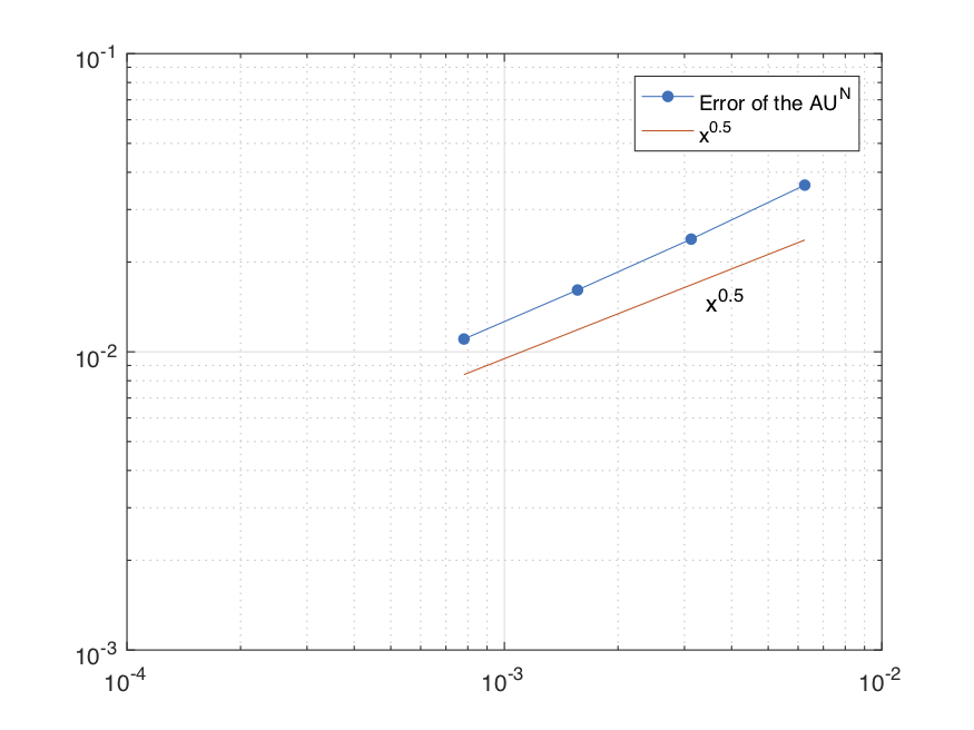
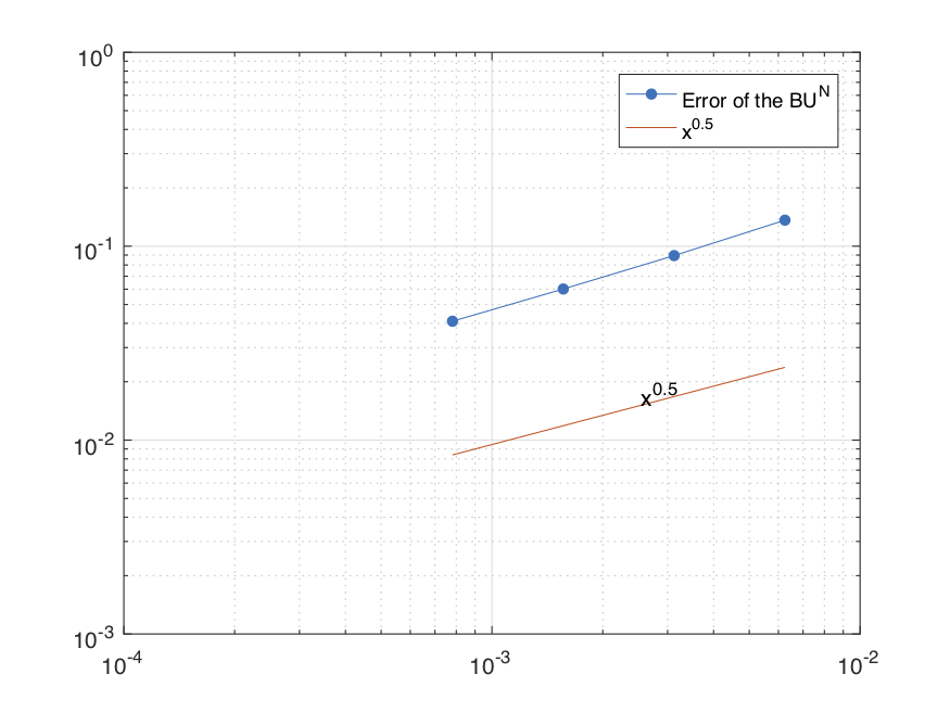
Fig. 1: Test 1: (a) The convergence rates $AU^{N}$; (b) the convergence rates $BU^{N}$.

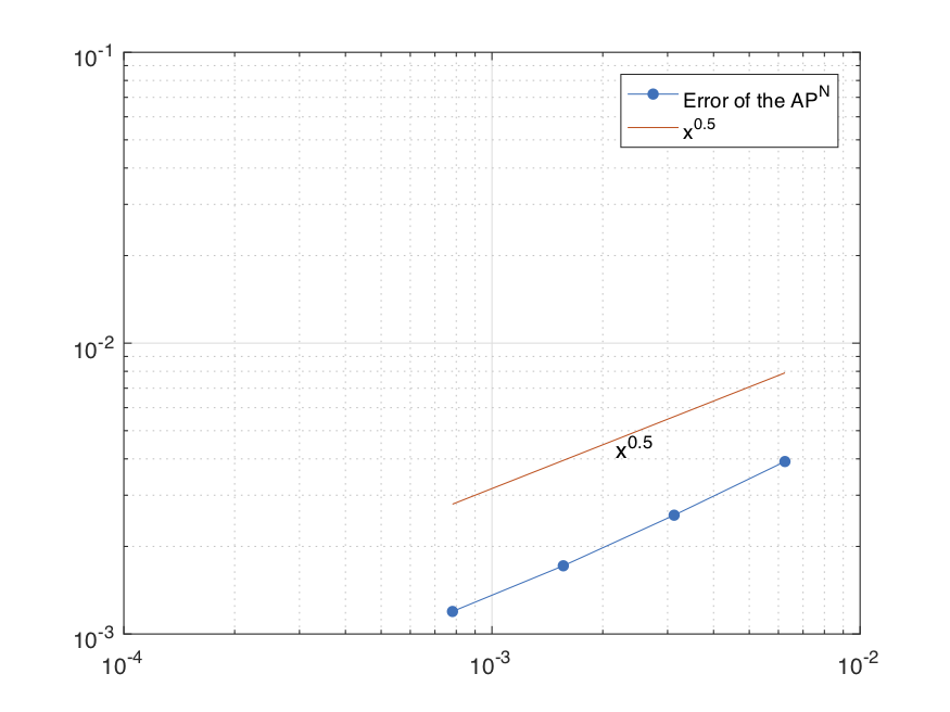
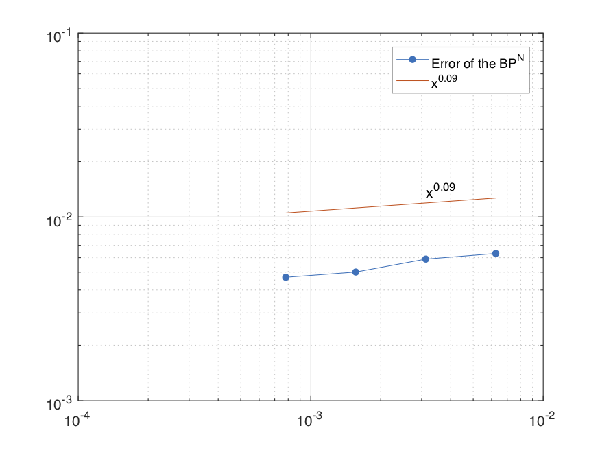
Fig. 2: Test 1: (a) The convergence rates $AP^{N}$; (b) the convergence rates $BP^{N}$.

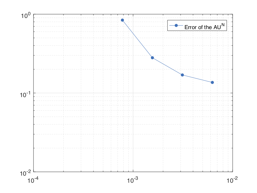
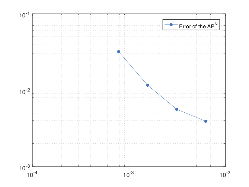
Fig. 3: Test 1: (a) The convergence rates $AU^{N}$; (b) the convergence rates $AP^{N}$.

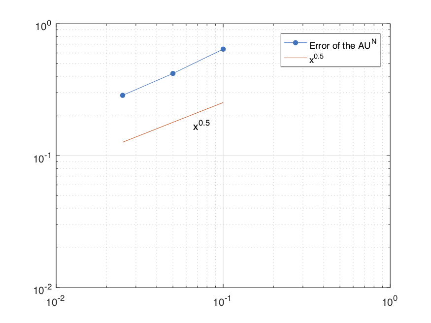
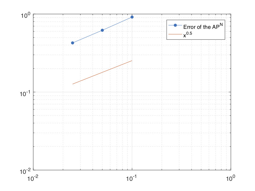
Fig. 4: Test 1: (a) The convergence rates $AU^{N}$; (b) the convergence rates $AP^{N}$.

Test 2. In the second numerical test, we compute the driven cavity flow on a unit square $(0,1)^{2}$. In this test the force function $f$ is chosen to be the constant zero-vector $(0,0)$. The no-slip boundary condition is only imposed on the part of the boundary $\{(x,1):0<x<1\}$ with the velocity $u=(1,0)$, and the zero Dirichlet condition is imposed on the rest of the boundary. The lowest order Taylor-Hood ($P_{2}-P_{1}$) element is used in this test. The same finite-dimensional Q-Wiener process as in Test 1 is used and we take $B(\cdot,u)=1$ and use the following parameters: $c=1$, $M=10$, $\nu=1$, $T=1$, $h=\frac{1}{20}$, $k=0.005$, and the realization number $N_{p}=5000$.

Figure 8 plots (a) the expected value of the pressure $p_{h}^{N}$; (b) the expected value of the velocity field $u_{h}^{N}$; (c) the streamlines of the expected value of $u_{h}^{N}$. Figures 8–Fig 8 show three computed samples of the pressure $p_{h}^{N}$ and the velocity $u_{h}^{N}$ as well as the streamlines of $u_{h}^{N}$. From Figure 8, we observe that the expectations of the pressure and velocity fields behave similarly to their deterministic counterparts, on the other hand, Figures 8–Fig 8 show that the stochastic pressure and velocity samples could be very different from their deterministic fields.

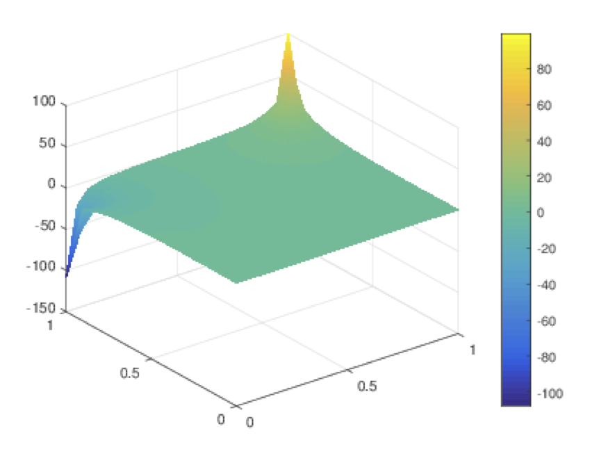
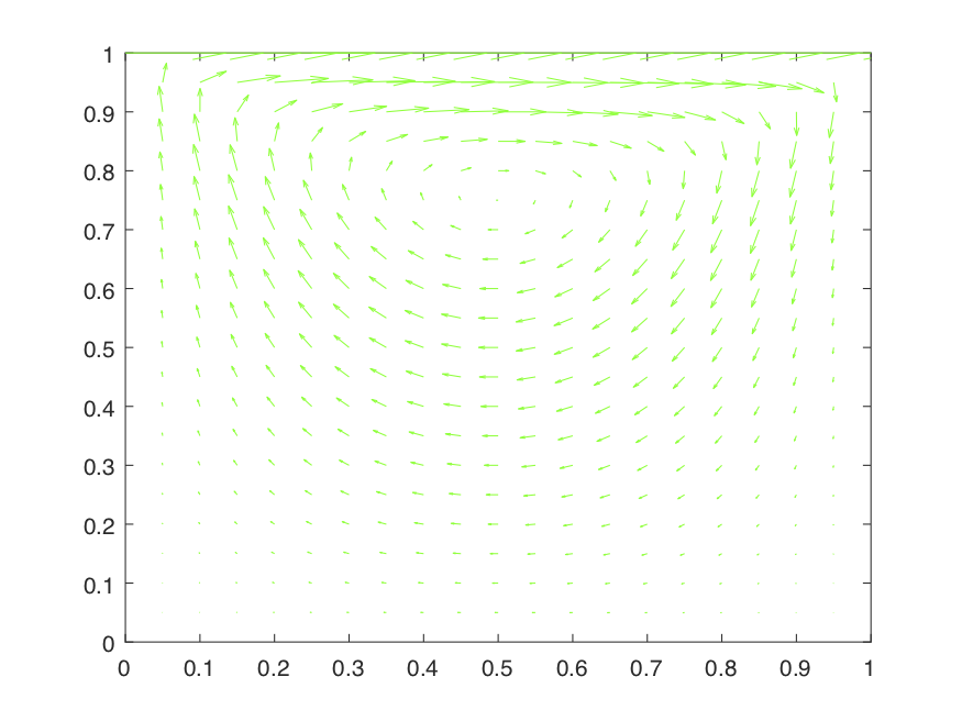
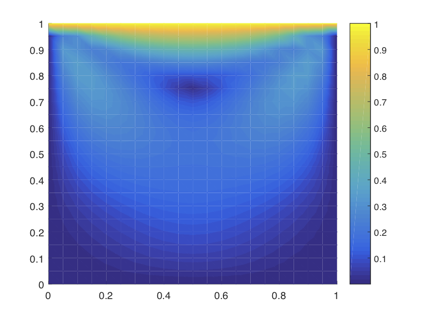
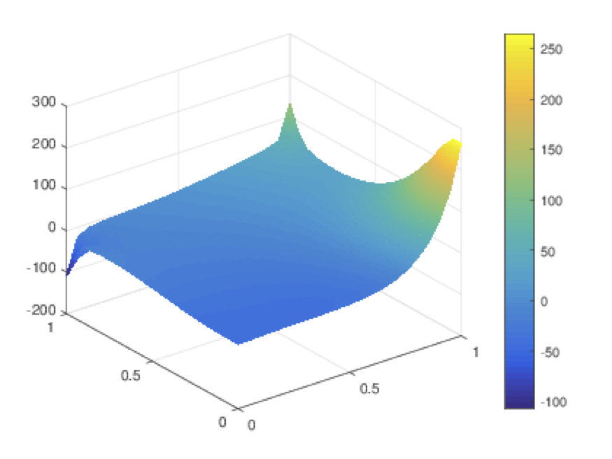
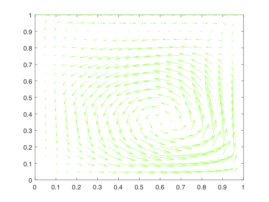
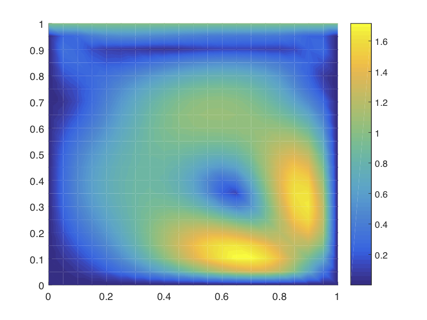
Fig. 5: Test 2: (a) The expected value of $p_{h}^{N}$; (b) the expected value of $u_{h}^{N}$; (c) the streamlines of the expected value of $u_{h}^{N}$.

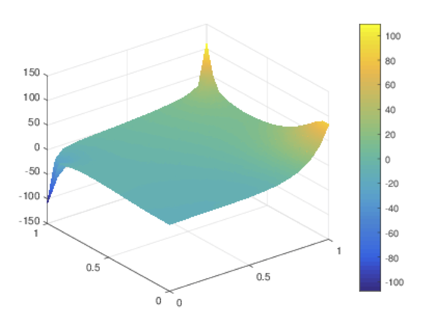
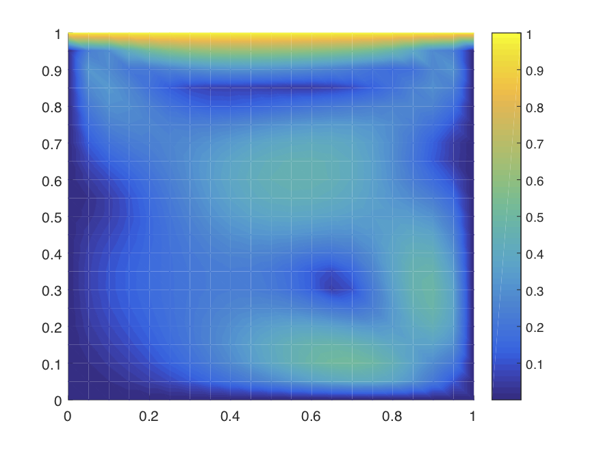
Fig. 6: Test 2: The first realization of (a) $p_{h}^{N}$; (b) $u_{h}^{N}$; (c) the streamlines of $u_{h}^{N}$.

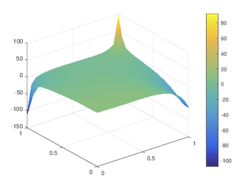
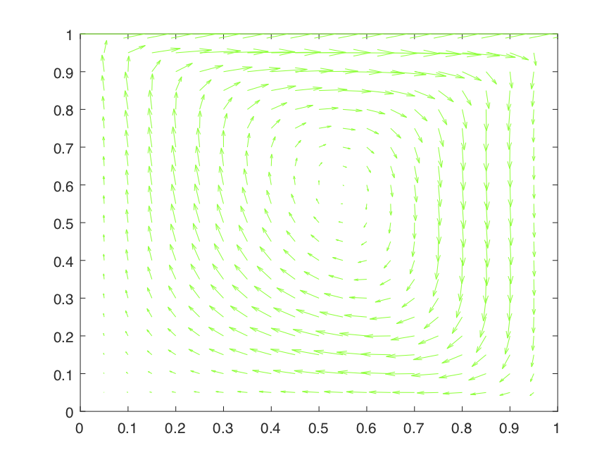
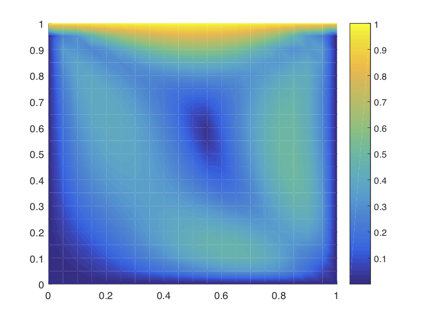
Fig. 7: Test 2: The second realization of (a) $p_{h}^{N}$; (b) $u_{h}^{N}$; (c) the streamlines of $u_{h}^{N}$.

Fig. 8: Test 2: The third realization of (a) $p_{h}^{N}$; (b) $u_{h}^{N}$; (c) the streamlines of $u_{h}^{N}$.

Acknowledgments. The authors would like to thank Professor Andreas Prohl of University of Tübingen (Germany) for his many stimulating discussions and critical comments as well as valuable suggestions which help to improve the early version of the paper considerably. In addition, his help on introducing and explaining several relevant references is also greatly appreciated.

References

- [1] R. A. Adams, Sobolev Spaces, 2nd Edition, Academic Press, 2003.
- [2] A. N.Douglas, L. R. Scott, and M. Vogelius, Regular inversion of the divergence operator with Dirichlet boundary conditions on a polygon, Ann. Scuola Norm. Sup. Pisa Cl. Sci., 15(2):169–192 (1988).
- [3] A. Bensoussan, Stochastic Navier-Stokes equations, Acta Appl. Math., 38:267–304 (1995).
- [4] A. Bensoussan and R. Temam, Equations stochastiques du type Navier-Stokes, J. Funct. Anal. 13, 195–222 (1973).
- [5] A. De Bouard and A. Debussche, A semi-discrete scheme for the stochastic nonlinear Schrödinger equation, Numer. Math., 96:733–770 (2004).
- [6] H. Bessaih, Z. Brzeźniak, and A. Millet, Splitting up method for the 2D stochastic Navier-Stokes equations, Stoch. PDE: Anal. Comp., 2:433–470 (2014).
- [7] H. Bessaih and A. Millet, On strong convergence of time numerical schemes for the stochastic 2D Navier-Stokes equations, arXiv:1801.03548 [math.PR], to appear in IMA J. Numer. Anal.
- [8] F. Brezzi and M. Fortin, Mixed and Hybrid Finite Element Methods, Springer, New York, 1991.
- [9] Z. Brzeźniak, E. Carelli, and A. Prohl, Finite element based discretizations of the incompressible Navier-Stokes equations with multiplicative random forcing, IMA J. Numer. Anal., 33:771–824 (2013).
- [10] Y. Cao, Z. Chen, M. Gunzburger, Error analysis of finite element approximations of the stochastic Stokes equations, Adv. Comput. Math., 33:215–230 (2010).
- [11] M. Capiński and S. Peszat, On the existence of a solution to stochastic Navier-Stokes equations, Nonlinear Anal., 44:141–177 (2001).
- [12] E. Carelli, E. Hausenblas and A. Prohl, Time-splitting methods to solve the stochastic incompressible Stokes equations, SIAM J. Numer. Anal., 50(6):2917–2939 (2012).
- [13] E. Carelli and A. Prohl, Rates of convergence for discretizations of the stochastic incompressible Navier-Stokes equations, SIAM J. Numer. Anal., 50(5):2467–2496 (2012).
- [14] P.-L. Chow, Stochastic Partial Differential Equations, Chapman and Hall/CRC, 2007.
- [15] T. A. Davis, Algorithm 832: UMFPACK V4.3-an unsymmetric-pattern multifrontal method. ACM Transactions on Mathematical Software. 30:196–199 (2004).
- [16] A. Ern and J.-L. Guermond, Theory and Practice of Finite Elements, Springer, 2004.
- [17] P. Dörsek, Semigroup splitting and cubature approximations for the stochastic Navier-Stokes equations, SIAM J. Numer. Anal., 50(2):729–746 (2012).
- [18] R. Falk, A Fortin operator for two-dimensional Taylor-Hood elements, ESAIM: Math. Model. Num. Anal., 42:411–424 (2008).
- [19] F. Flandoli, Stochastic differential equations in fluid dynamics, Rend. Sem. Mat. Fis. Milano, 66:121–148 (1996).
- [20] F. Flandoli and D. Gatarek, Martingale and stationary solutions for stochastic Navier-Stokes equations, Probab. Theory Related Fields, 102:367–391 (1995).
- [21] M. Hairer, and J. C. Mattingly, Ergodicity of the 2D Navier-Stokes equations with degenerate stochastic forcing, Ann. of Math., 164:993–1032 (2006).
- [22] José A. Langa, José Real, Jacques Simon, Existence and Regularity of the Pressure for the Stochastic Navier-Stokes Equations, Appl. Math. Optim., 48:195–210 (2003).
- [23] F. Hecht, A. LeHyaric, O. Pironneau, Freefem++ version 2.24-1, http://www.freefem.org/ff++, 2008.
- [24] V. Girault and P.-A. Raviart, Finite Element Methods for Navier-Stokes Equations, Springer, New York, 1986.
- [25] I. Gyöngy and A. Millet, Rate of convergence of implicit approximations for stochastic evolution equations, Potential Anal., 30:29–64 (2009).
- [26] J. A. Langa, J. Real, and J. Simon, Existence and regularity of the pressure for the stochastic Navier-Stokes equations, Appl. Math. Optim., 48:195–210 (2003).
- [27] U. Manna, J. L. Menaldi, and S. S. Sritharan, Stochastic 2-D Navier-Stokes equation with artificial compressibility, Commun. Stoch. Anal., 1:123–139 (2007).
- [28] G. Da Prato and J. Zabczyk, Stochastic Equations in Infinite Dimensions, Cambridge University Press, Cambridge, UK, 1992.
- [29] J. Printems On the discretization in time of parabolic stochastic partial differential equations, ESAIM: M2AN 35(6):1055–1078 (2001).
- [30] R. Temam, Navier-Stokes Equations. Theory and Numerical Analysis, 2nd ed., AMS Chelsea Publishing, Providence, RI, 2001.
- [31] X. Yang, Y. Duan and Y. Guo, A posteriori error estimates for finite element approximation of unsteady incompressible stochastic Navier-Stokes equations, SIAM J. Numer. Anal., 48, 1579–1600 (2010).