Transferring Multiscale Map Styles Using Generative Adversarial Networks

Abstract

The advancement of the Artificial Intelligence (AI) technologies makes it possible to learn stylistic design criteria from existing maps or other visual art and transfer these styles to make new digital maps. In this paper, we propose a novel framework using AI for map style transfer applicable across multiple map scales. Specifically, we identify and transfer the stylistic elements from a target group of visual examples, including Google Maps, OpenStreetMap, and artistic paintings, to unstylized GIS vector data through two generative adversarial network (GAN) models. We then train a binary classifier based on a deep convolutional neural network to evaluate whether the transfer styled map images preserve the original map design characteristics. Our experiment results show that GANs have great potential for multiscale map style transferring, but many challenges remain requiring future research.

1 Introduction

A map style is an aesthetically cohesive and distinct set of cartographic design characteristics (Kent and Vujakovic,, 2009). The map style sets the aesthetic tone of the map, evoking a visceral, emotional reaction from the audience based on the interplay of form, color, type, and texture (Gao et al.,, 2017; Roth, forthcoming, ). Two maps can have a very different look and feel based on their map style, even if depicting the same information or region (Figure 1; see Stoter, (2005); Kent and Vujakovic, (2009) for comparisons of in-house styles of national mapping agencies). Arguably, map styling—and the myriad design decisions therein—is a primary way that the cartographer exercises agency, authorship, and subjectivity during the mapping process (see Buckley and Jenny, (2012) for recent discussions on aesthetics, style, and taste).

Increasingly, web cartographers need to develop a coherent and distinct map style that works consistently across multiple map scales to enable interactive panning and zooming of a “map of everywhere” (Roth et al.,, 2011). Such multiscale map styling taps into a rich body of research on generalization and multiple representation databases in cartography (see Mackaness et al., (2011) for a compendium developed by the ICA Commission on Generalization). A large number of generalization taxonomies now exist to inform the multiscale map design process (e.g., DeLucia and Black, (1987); Christophe et al., (2016); McMaster and Shea, (1992); Regnauld and McMaster, (2007); Foerster et al., (2007); Stanislawski et al., (2014); Raposo, (2017); Shen et al., (2018)), most of which focus on vector geometry operations for meaningfully removing detail in geographic information (e.g., simplify, smooth, aggregate, collapse, merge).

Brewer and Buttenfield, (2007) argue that adjusting the symbol styling can have as great an impact in the legibility of multiscale map designs as other selection or geometry manipulations. Accordingly, Roth et al., (2011) discuss how cartographers can manipulate the visual variables, or fundamental building blocks of graphic symbols (e.g., shape, size, orientation, dimensions of color like hue, value, saturation, and transparency), to promote legibility and maintain a coherent style across map scales. A number of web mapping services and technologies now exist to develop and render such multiscale map style rules as interlocking tilesets, such as CartoCSS, Mapbox Studio,TileMill, or TileCache. Beyond authoritative or classic map styles (see Muehlenhaus, (2012) for a review), these tools enable multiscale web map styling that is exploratory, playful, and even subversive (for instance, see Christophe and Hoarau, (2012) for examples of multiscale map styling using Pop Art as inspiration). Despite these advances, establishing a map style that works across regions and scales remains a fundamental challenge for web cartography, given the wide array of stylistic choices available to the cartographer and the limited guidance for integrating creative, artistic styles into multiscale maps like Google Maps and OpenStreetMap (OSM).

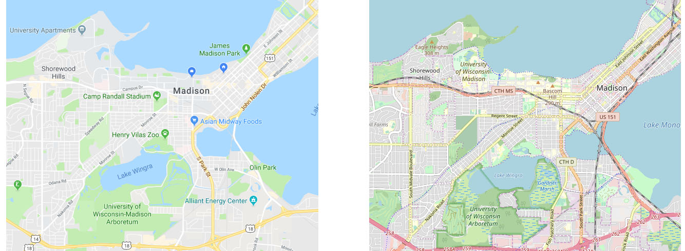
Figure 1: The Google Maps (left) and OpenStreetMap (right) styles for Madison, Wisconsin (USA). Google Maps has a flatter visual hierarchy to emphasize labels and points of interests as well as enable vector overlays, whereas OpenStreetMap is more visually complex and includes a wider variety of features and symbols.

Here, we ask if artificial intelligence (AI) can help illuminate, transfer, and ultimately improve multiscale map styling for cartography, automating some of the multiscale map style recreation and assisting the cartographer in developing novel representations. Our work draws from the active symbolism paradigm in cartography and visualization (Armstrong and Xiao,, 2018), in which “the production of maps switches from a sequence of actions taken by a mapmaker to a process of specifying criteria that are used to create maps using intelligent agents”. Specifically, whether AI can learn map design criteria from existing map examples (or visual art) and then transfer these criteria to new multiscale map designs.

Latest AI technology advancements in the past decade include a range of deep learning methods developed primarily in computer science for image classification, segmentation, objection localization, style transfer, natural language processing, and so forth (LeCun et al.,, 2015; Goodfellow et al.,, 2016; Gatys et al.,, 2016). Recently, GIScientists and cartographers, along with computer scientists have been investigating various AI and deep learning applications such as geographic knowledge discovery (Mao et al.,, 2017; Hu et al.,, 2018), map-type classification (Zhou et al.,, 2018), scene classification (Zou et al.,, 2015; Srivastava et al.,, 2018; Law et al.,, 2018; Zhang et al.,, 2018, 2019), scene generation (Deng et al.,, 2018), automated terrain feature identification from remote sensing imagery (Li and Hsu,, 2018), automatic alignment of geographic features in contemporary vector data and historical maps (Duan et al.,, 2017), satellite imagery spoofing (Xu and Zhao,, 2018), spatial interpolation (Zhu et al.,, 2019), and environmental epidemiology (VoPham et al.,, 2018). Relevant to our work on multiscale map style, a new class of AI algorithms called generative adversarial networks (GANs) have been developed to generate synthetic photographs that mimic real ones (Goodfellow et al.,, 2014). The GANs input real photographs to train the model, and the resulting output photographs look at least superficially authentic to human observers, suggesting a potential application for the multiscale map styling. Several promising studies have used GANs combined with multi-layer neural networks to transfer the styles of existing satellite imagery and vector street maps (Isola et al.,, 2017; Zhu et al.,, 2017; Xu and Zhao,, 2018; Ganguli et al.,, 2019). However, several research questions and uncertainty concerns remain. First, which feature types, symbol styling, and zoom levels best enable map style transfer? Second, which AI algorithm or combinations of algorithms work best for map style transfer? Finally, how usable are the resulting maps after style transfer; do the results appear as authentic maps or not?

To this end, we propose a novel framework to transfer existing style criteria to new multiscale maps using GANs without the input of CartoCSS map style configuration sheets. Specifically, the GANs learn (1) which visual variables encode (2) which map features and distributions at (3) which zoom levels, and then replicate the style using the most salient combinations. In order to evaluate the results of our framework, we then train a deep convolutional neural network (CNN) classifier to judge whether the outputs with transferred map styling still preserve the input map characteristics.

The paper proceeds with four additional sections. In Section 2, we describe the methods framework, including data collection and preprocessing, tiled map generation, and the paired and unpaired GAN models based on Pix2Pix and CycleGAN respectively. We then describe in Section 3 an experiment using geospatial features in Los Angeles and San Francisco (USA) to test the feasibility and accuracy of our framework. Specifically, we provide both a qualitative visual assessment and quantitative assessment of two different GAN models, Pix2Pix and CycleGAN, at two different map scales. We discuss potential applications with challenges in Section 4 and offer conclusions and future work in Section 5.

2 Methods

2.1 Overview

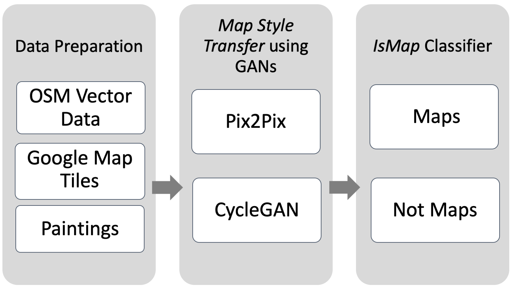
Figure 2: The methodology framework for map style transfer and evaluation: (1) data preparation, (2) map style transfer using GANs, (3) IsMap classifier.

Our proposed methods framework includes three stages as shown in Figure 2. First, we prepare unstyled or “raw” GIS vector data from a geospatial data source that we wish to style (here OpenStreetMap (OSM) vector data, which is given an initial simple styling for the purpose of visual display; details below) as well as example styled data sources we wish to reproduce and transfer (here Google Maps tiles and painted visual art). Second, we configure two generative adversarial network methods to learn the multiscale map styling criteria: Pix2Pix, which uses paired training data between the target and example data sources, and CycleGAN, which can use unpaired training data (details below). Third, we employ a deep convolutional neural network (CNN) classifier (described as IsMap below) to judge whether the outputs with transferred map styling do or do not preserve map characteristics (Krizhevsky et al.,, 2012; Evans et al.,, 2017).

2.2 Data Preparation and Preprocessing

Our framework requires two types of map layers as inputs: we refer to these as simple styled maps and target styled maps. We generate the transfer styled maps by incorporating the geographic features from simple styled maps with the aesthetic styles of the target styled maps. We then collect and generate the input map layers as raster web map tilesets that comprise square images, but contain styling symbols that represent different types of geographic features (e.g., buildings, lakes, roads, and so on).

Tiled map services are among the most popular web mapping technologies for representing geographical information at multiple scales (Roth et al.,, 2015). Such web map tilesets interlock using a multi-resolution, hierarchical pyramid model. Within this pyramid model, map scale is referred to as zoom level and expressed in 1-20 notation, with 1 denoting the smallest cartographic scale (i.e., zoomed out) and 20 the largest cartographic scale (i.e., zoomed in). While the spatial resolution gets coarser from the top to the bottom of the tile pyramid, the size of each image tile in the tileset remains across zoom levels (Peterson,, 2011, 2014), typically captured at 256x256 pixels (8-bit). Therefore, serving pre-rendered image tiles typically is less computationally demanding than dynamically rendering vector map tiles in the browser. We used two popular tilesets for this study: OpenStreetMap, which we downloaded in raw vector format without any map styles and served as a tiled web service for the simple styled maps case using GeoServer, and Google Maps, which we acquired using their API as the target styled maps case. Within OSM data, multiple classes of features exist for each geometry type (i.e., point, line, and polygon). For the simple styled maps, we rendered these different classes using different colors and subtle transparency so that they could be visually discriminated in the resulting tileset. We used the Spherical Mercator (EPSG:900913) coordinate system for georeferencing the OSM tiles to ensure they aligned with the Google Maps tileset.

2.3 GANs

Next, we utilized the GANs to generate transfer styled map images by combining the geographic features of the simple styled maps and the learned map style from the target styled maps. GANs have two primary components (Goodfellow et al.,, 2014): the generator $G$, which generates fake outputs that mimic real examples using the upsampling vectors of random noise, and the discriminator $D$, which distinguishes the real and fake images according to the downsampling procedure. Following the format of an adversarial loss, $G$ iterates through a present number of epochs (an entire dataset is passed forward and backward in one epoch through the deep learning neural network) and becomes optimized when the visual features of the reproduced transfer images have a similar distribution with the ground truth target style and the fake images generated by $G$ cannot be distinguished by the discriminator $D$. The training procedures of both $G$ and $D$ occur simultaneously.

$$\operatorname*{min}_{G}\operatorname*{max}_{D}V(D,G)=\mathbb{E}_{x{\sim}p_{data}(x)}[logD(x)]+$$ (1)

$$\mathbb{E}_{z{\sim}p_{z}(z)}[log(1-D(G(z))]$$

where $x$ is a real image and $z$ is the random noise.

Since the original GAN aims at generating fake images that have a similar distribution of features in the entire training dataset, it may not be suitable for generating specific types of images under certain conditions. Therefore, Mirza and Osindero, (2014) proposed the Conditional GAN (C-GAN) with auxiliary information to generate images with specific information. Different from the original GAN, the C-GAN adds hidden layers $y$ that contain extra conditional information in generator $G$ and discriminator $D$. The objective function is as:

$$\operatorname*{min}_{G}\operatorname*{max}_{D}V(D,G)=\mathbb{E}_{x{\sim}p_{data}(x)}[logD(x|y)]+$$ (2)

$$\mathbb{E}_{z{\sim}p_{z}(z)}[log(1-D(G(z|y))]$$

The auxiliary information in the C-GAN can take many forms of input, such as categorical labels that generate images in a specific category (e.g., food, railways; Mirza and Osindero, (2014)), and embedded text to generate images from annotations (Reed et al.,, 2016). For multiscale map styling, the target styled maps represent auxiliary information, making the C-GAN more suitable for our research.

There are two popular types of C-GAN: paired and unpaired. Paired C-GAN uses image-to-image translation to train a model on two paired groups of images, with output combining content from one image and the style from the other image. Unpaired C-GAN also completes an image-to-image translation, but with the transfer of images between two related domains $X$ and $Y$ in the absence of paired training examples. In this research, we tested both methods, using the Pix2Pix and the CycleGAN respectively, to examine their suitability for multiscale map style transfer.

2.4 Pix2Pix

Pix2Pix is a paired C-GAN algorithm that learns the relationship between the input images and the output images based on the paired-image training set (Isola et al.,, 2017). In addition to minimizing the objective loss function of general C-GAN, the Pix2Pix generator trains not just to fool the discriminator, but also to produce ground truth-like output. The objective function of the extra generator is defined as:

$$\mathcal{L}_{L1}(G)=\mathbb{E}_{x,y,z}[\parallel y-G(x,z)\parallel_{1}]$$ (3)

By combing the two objective functions, the final objective function is computed as:

$$\mathcal{L}_{Pix2Pix}=\mathcal{L}_{cGAN}(G,D)+\lambda\mathcal{L}_{L1}(G)$$ (4)

For this research, we paired the OpenStreetMap and Google Maps tiles for the same locations and at the same zoom levels as the input dataset for training the Pix2Pix model.

2.5 CycleGAN

Pix2Pix is appropriate for pairing two map tilesets containing the same geographic extents and scales. However, Pix2Pix cannot transfer a target artistic style from non-map examples (e.g., a Monet painting) to a map tileset. Compared with Pix2Pix, CycleGAN learns the style from one specific source domain (different styles of images) and transfer to a target domain (Zhu et al.,, 2017). In other words, CycleGAN does not require two input images with the same geographic extent, but instead just two input training datasets that have different visual styles. CycleGAN establishes two associations to achieve the style transfer: $G:X$$\,\to\,$$Y$ and $F:Y$$\,\to\,$$X$. Two adversarial discriminators $D_{X}$ and $D_{Y}$ are trained respectively, where $D_{X}$ distinguishes the images in dataset $X$ and images generated by $F(y)$, and $D_{Y}$ distinguishes the images in dataset $Y$ and images generated by $G(x)$. The objective function for establishing the relationship of the images in domain $X$ to domain $Y$ is represented as:

$$\mathcal{L}_{GAN}(G,D_{Y},X,Y)=\mathbb{E}_{y\sim p_{data}(y)}[logD_{Y}(y)]$$ (5)

$$+\mathbb{E}_{x\sim p_{data}(x)}[log(1-D_{Y}(G(x))]$$

A similar adversarial loss for transforming the images in domain $Y$ to another domain $X$ is introduced as $\mathcal{L}_{GAN}(F,D_{X},Y,X)$, where $G$ generates images that look similar to the images in the other domain, and $D$ distinguishes the fake images and the real images. CycleGAN also introduces an extra loss called the cycle consistency loss. After $G$ and $F$ generate images with the similar distribution to the input domain, the cycle consistency loss guarantees when input the images generated to the other generator, the generated images can be restored to the original domain. In other words, $x\to G(x)\to F(G(x))\approx x$. More details can be found in Zhu et al., (2017). The cycle consistency loss is expressed as:

$$\mathcal{L}_{cyc}(G,F)=\mathbb{E}_{x\sim p_{data}(x)}[\parallel F(G(x))-x\parallel_{1}]$$ (6)

$$+\mathbb{E}_{y\sim p_{data}(y)}[\parallel G(F(y))-y\parallel_{1}]$$

By combining the two adversarial losses and the cycle consistency loss, the full objective function is expressed as:

$$\mathcal{L}_{CycleGAN}=\mathcal{L}_{GAN}(G,D_{Y},X,Y)$$ (7)

$$+\mathcal{L}_{GAN}(F,D_{X},Y,X)$$

$$+\lambda\mathcal{L}_{cyc}(G,F).$$

2.6 IsMap Classifier

Again, GANs’ success in map style transfer relies on the adversarial loss forcing the generated maps to be indistinguishable from the input target-styled maps. In addition to the loss curve reported in the model training process, we employ a deep CNN-based binary classifier called IsMap to judge whether the transfer styled maps are perceived as maps (Evans et al.,, 2017). CNNs can produce significant improvements in image classification tasks compared with other machine learning models (Huang et al.,, 2017; Maggiori et al.,, 2017). However, the deeper the neural network, the greater the computational costs. Based on existing literature review and comparison on ImageNet, we chose the GoogleNet/Inception-v3 deep neural network model. More details about the GoogleNet/Inception architecture is available in Szegedy et al., (2016).

We created two categories for preparing the training dataset for the IsMap classifier: maps and photos. We randomly selected those styled map tiles collected in Section 2.1 as positive samples. We did not include the map tiles used for training the classifier in the style transferring process. In addition, we randomly collected Flickr photos from its search API without map content as negative samples. We resized all maps and photos into consistent 256*256 pixel images (Figure 3).

2.7 Evaluation

After training the aforementioned two C-GAN models, we evaluated the performance of each model based on the IsMap classifier. The IsMap classifier returns four results: true positive (TP), true negative (TN), false positive (FP), and false negative (FN). TP indicates the number of transfer styled maps correctly classified as a map and TN indicates the number of tested photos correctly classified as a photo. FP indicates the number of testing photos incorrectly predicted as maps and FN indicates the number of transfer styled maps incorrectly predicted as photos. We then calculated the following four metrics based on the IsMap output:

1. Precision: The portion of the transfer styled images correctly labeled as maps in all output maps, using the following equation:

   $$Precision=\frac{TP}{TP+FP}$$ (8)

2. Recall: The portion of true positives captured in classification compared to all actual maps in the labeling process, using the following equation:

   $$Recall=\frac{TP}{TP+FN}$$ (9)

3. Accuracy: The portion of images labeled correctly either as maps or as photos, using the following equation:

   $$Accuracy=\frac{TP+TN}{TP+TN+FP+FN}$$ (10)

4. F1 score: Combines both precision and recall values to measure the overall accuracy, using the following equation:

   $$F1=2*\frac{Precision*Recall}{Precision+Recall}$$ (11)

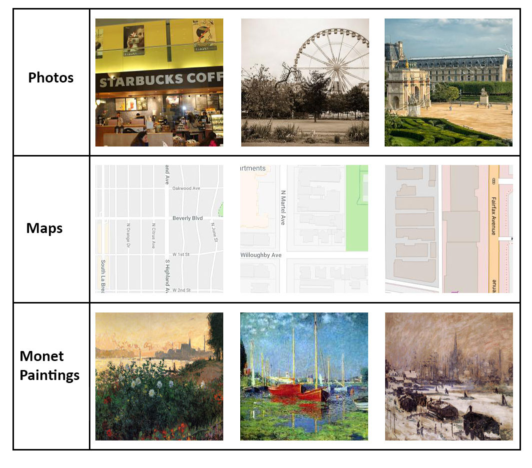
Figure 3: Categories of dataset for training and testing. The first row shows examples of photos collected from Flickr, the second row shows examples of tiled images from both Google Maps and OpenStreetMap, the last line show examples of Monet paintings.

3 Experiment and Results

3.1 Input Datasets

We conducted experiments using the OSM raw vector data as well as Google Maps with two C-GAN models for two U.S. metropolitan areas to test the feasibility and accuracy of our framework. We utilized the same training and testing datasets for both the Pix2Pix and CycleGAN models to compare their performance. Because OSM vector data coverage varies considerably across regions, we focused on two major cities with high quality data: Los Angeles and San Francisco. We downloaded the OSM vector data for these cities from Geofabrik and served the simple styled maps as map tiles using TileCache and GeoServer. To simplify the experiment further, we generated map tiles at only two zoom levels 15 and 18, matching the spatial resolution with the target styled maps from Google Maps. In total, we generated 870 simple styled maps tiles at zoom level 15, and 9,156 image tiles at zoom level 18 for use as the C-GAN training sets. We paired the simple-style maps with the equivalent Google Maps tiles for the Pix2Pix model.

After finishing the training process using the two C-GAN models, we randomly selected 217 and 257 simple styled maps tiles, from zoom levels 15 and 18 respectively, to receive the transferred style as testing cases. These selected simple styled maps tiles were not included in the C-GAN training process, and thus did not influence style learning and only used for validation.To train the GoogleNet-based CNN classifier IsMap, we downloaded 5,500 photos without map content from Flickr, and 500 tiled maps from both Google Maps and OSM styled maps at different zoom levels. We then trained the IsMap classifier using this sample to produce the binary label of True or False.

3.2 Pix2Pix: Style Transferring with Paired Data

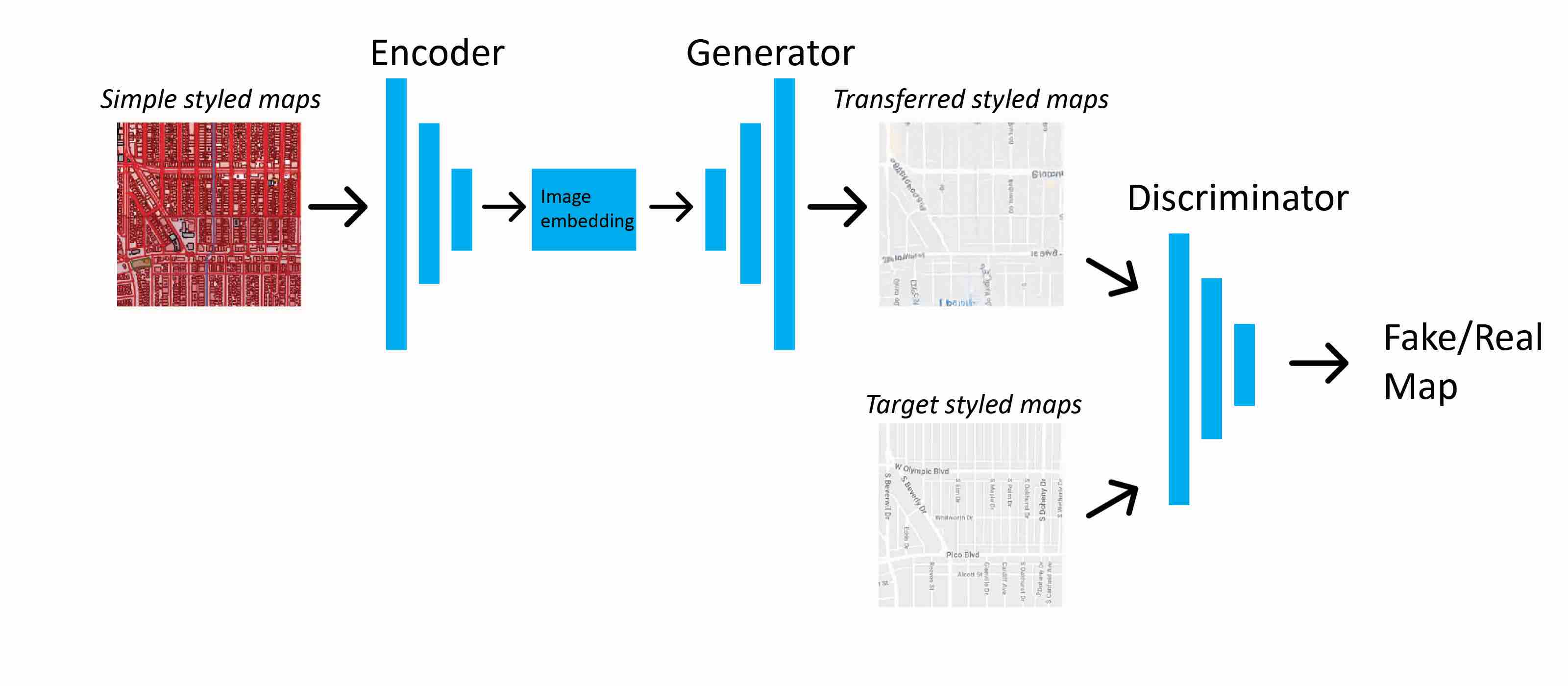
Figure 4: Data flow of Pix2Pix in this research.

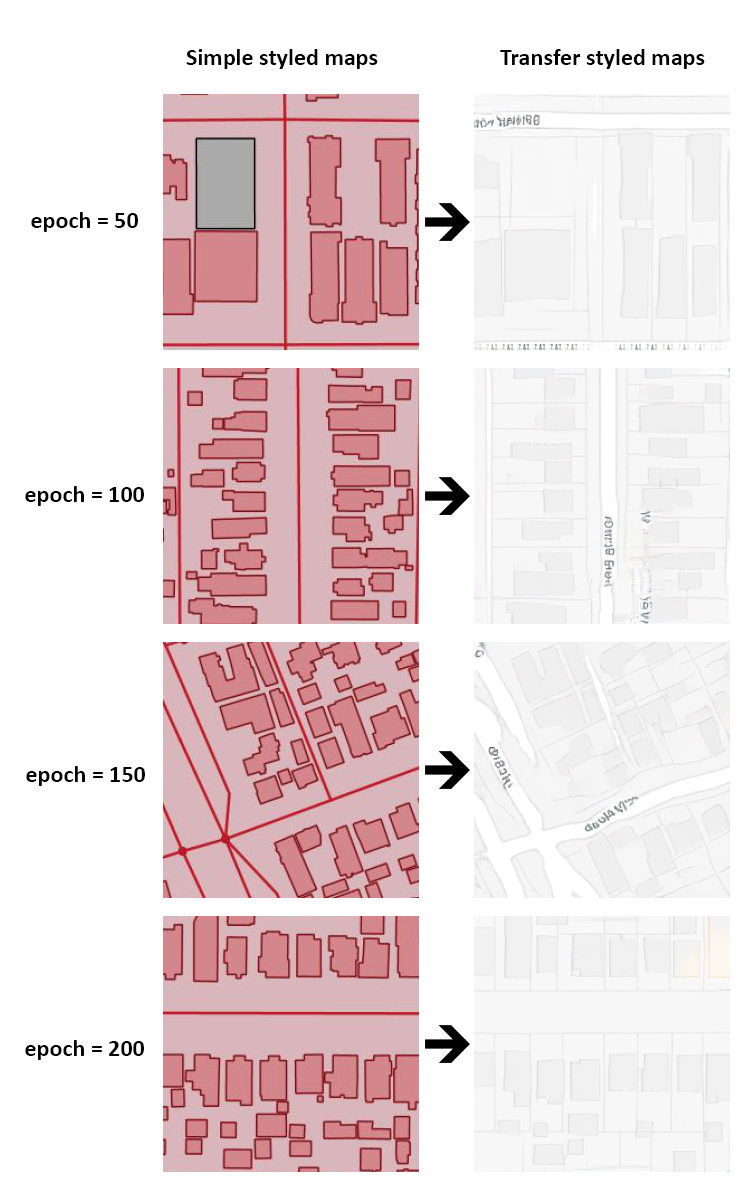
Figure 5: Training process using Pix2Pix at zoom level 18. Examples of simple styled maps and target styled maps in epoch 50, 100, 150 and 200 are shown individually.

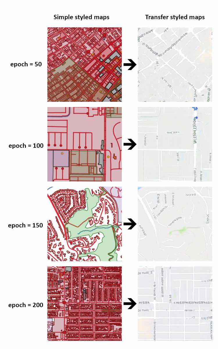
Figure 6: Training process using Pix2Pix at zoom level 15. Examples of simple styled maps and target styled maps in epoch 50, 100, 150 and 200 are shown individually.

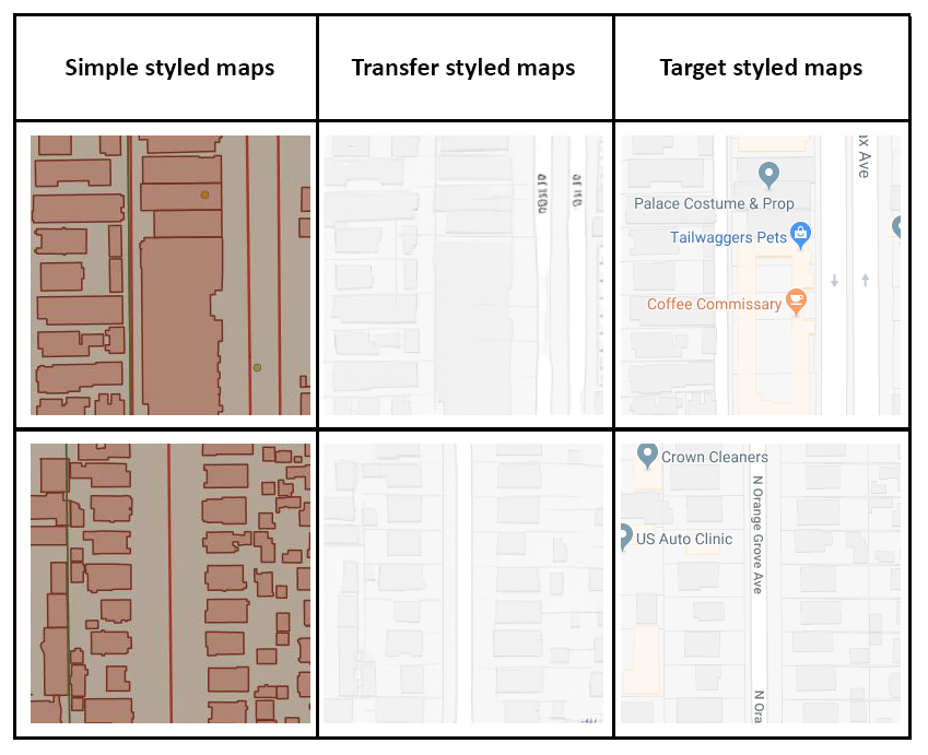
Figure 7: Results of the map style Transfer using Pix2Pix at zoom level 18. Examples of simple styled maps are shown in the first column, transfer styled maps based on Pix2Pix are shown in the second column, and the target styled maps from Google Maps are shown in the last column.

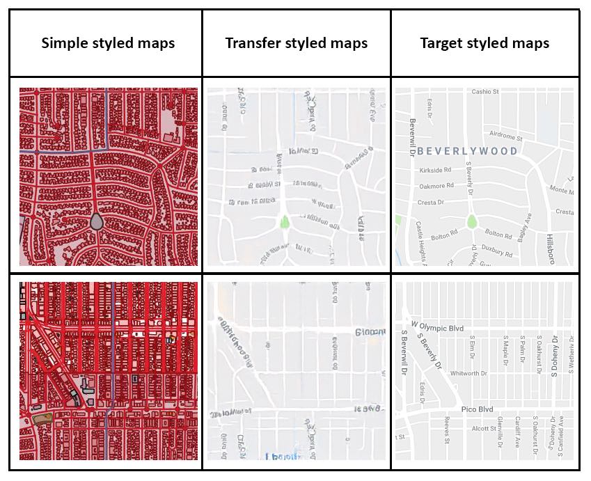
Figure 8: Results of the map style transfer using Pix2Pix at zoom level 15. Examples of simple styled maps are shown in the first column, transfer styled maps based on Pix2Pix are shown in the second column, and the target styled maps from Google Maps are shown in the last column.

Figure 4 illustrates the training process for the Pix2Pix model. First, we created the simple styled maps tiles from the OSM vector data, and then fed these tiles into the generator $G$ by encoding and embedding those images as vectors to generate the “fake” transfer styled maps. Then, we input the generated target styled maps and the transfer styled maps into the discriminator $D$, which iterated through 200 epochs until the discriminator no longer delineate the real versus fake maps. Figures 5 and 6 provide examples of Pix2Pix transfer styled maps tiles at 50, 100, 150, and 200 epochs for zoom level 18 and 15 respectively.

3.2.1 Generative Process with Map Tiles at a Large Scale

Figure 7 depicts Pix2Pix transfer styled maps generated at zoom level 18. Intuitively, the transfer styled maps look similar to the Google Maps tiles, which proves the basic feasibility of our AI framework broadly and the utility of Pix2Pix C-GAN model specifically. Compared with the original simple styled tiled maps, Pix2Pix preserves the detailed geometry of the roads and buildings with minimal observed generalization, but fails to maintain legible labels and colored markers (see discussion below). Notably, Pix2Pix consistently applies the target white road styling with a consistently line thickness to input line features and also applies the target grey building styling with rigid corners to input rectangular features, showing a relationship between salient visual variables and feature types in the transfer style generative process.

3.2.2 Generative Process with Tiles at a Small Scale

Figure 8 shows Pix2Pix transfer styled maps at zoom level 15. Compared with the original simple styled maps, Pix2Pix overgeneralizes the geometry of road features at zoom level 15, with many intermediate-size streets removed from the target styled maps. This overgeneralization potentially is explained by differences in the vector data schemas between OSM and Google Maps, resulting in a thinner road network in the OSM-based transfer styled maps. In comparison, Pix2Pix appropriately thinned the building features in the transfer styled maps, eliminating most buildings at zoom level 15 compared to zoom level 18 based on differences in the target styled maps. Thus, Pix2Pix is reasonably successful at multiscale generalization and style transfer, with the Pix2Pix model preserving feature types from the simple styled maps that are most salient in the target styled maps when changing zoom levels.

3.2.3 Limitations of the Pix2Pix

Although the generated transfer styled maps are similar to the target styled maps at both zoom levels, several limitations in the output exist. First, the map labels are important parts of the target styled maps, but are not preserved in the transfer styled maps, a major shortcoming of the image-based Pix2Pix model. Thus, while labeling and annotation falls outside of style learning, Pix2Pix does still learn knowledge of where to put the labels on the map for subsequent manual label placement. Second, Pix2Pix does not preserve less frequently observed colors in the target styled maps, such as the colored markers in Figure 7, instead basing the style transfer on the most common colors in the target style. Accordingly, the transfer styled maps does not capture grassland, lakes, etc., compared to the road and building colors dominating the urban landscapes of Los Angeles and San Francisco. However, color sensitivity may improve when expanding the geographic extent, and thus feature diversity, of the tilesets.

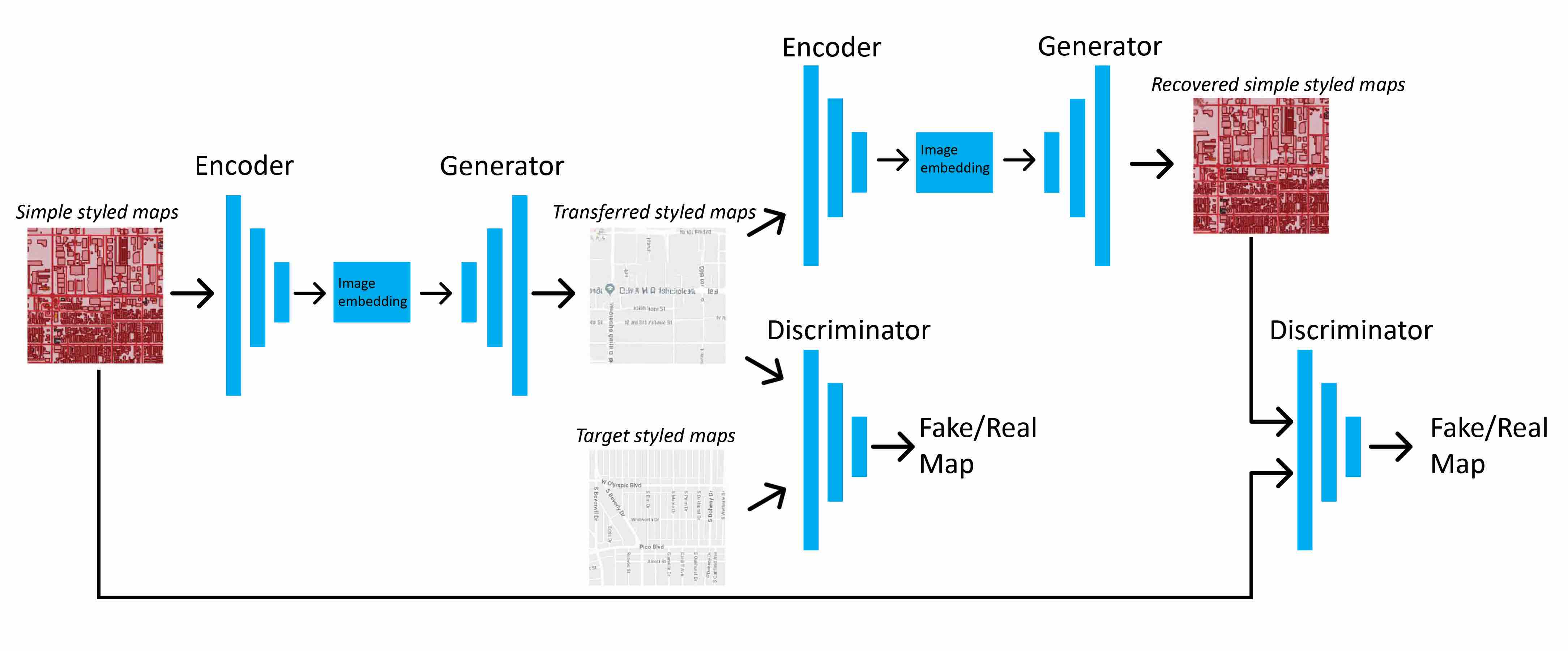
Figure 9: Data flow of CycleGAN in this research.

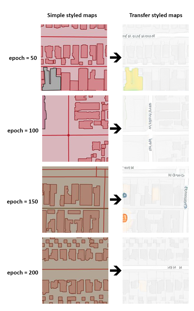
Figure 10: Training process using CycleGAN at zoom level 18. Examples of simple styled maps and target styled maps in epoch 50, 100, 150 and 200 are shown individually.

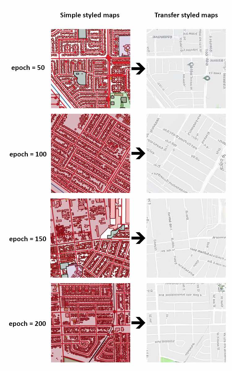
Figure 11: Training process using CycleGAN at zoom level 15. Examples of simple styled maps and target styled maps in epoch 50, 100, 150 and 200 are shown individually.

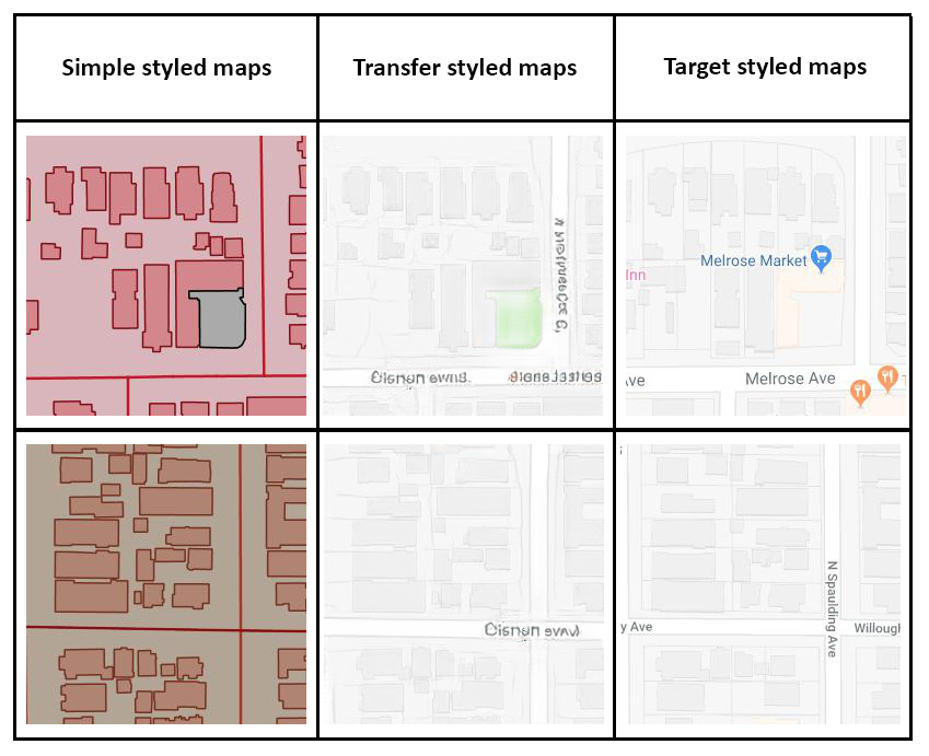
Figure 12: Results of the map style transfer using CycleGAN at zoom level 18. Examples of simple styled maps are shown in the first column, transfer styled maps based on CycleGAN are shown in the second column, and the target styled maps from Google Maps are shown in the last column.

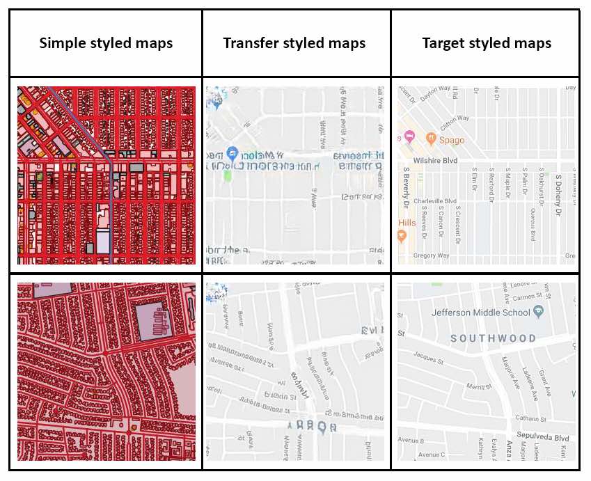
Figure 13: Results of the map style transfer using CycleGAN at zoom level 15. Examples of simple styled maps are shown in the first column, transfer styled maps based on CycleGAN are shown in the second column, and the target styled maps from Google Maps are shown in the last column.

3.3 CycleGAN Style Rendering with Unpaired Data

Figure 9 illustrates the training process for the CycleGAN model. Similar to the Pix2Pix training, we encoded the OSM vector data to create the simple styled maps tiles. These simple styled maps are used as input to generator $G$ to produce transfer styled maps and also represent knowledge that can be restored for discriminator $D$. Again, CycleGAN does not used paired data, with the target styled maps generated using randomly selected images from Google Maps. Similar to the Pix2Pix model training, we also trained the CycleGAN model across 200 epochs, enabling comparison performance between the two models. Figures 10 and 11 provide examples of CycleGAN transfer styled maps tiles at 50, 100, 150, and 200 epochs for zoom level 18 and 15 respectively.

3.3.1 Generative Process with Tiles at a Large Scale

Figure 12 shows CycleGAN transfer styled maps generated at zoom level 18. CycleGAN preserves the shapes of roads and building well. Notably, CycleGAN includes marker overlays from the target styled maps in some of the transfer styled maps, a benefit over Pix2Pix, although the colors and locations are incorrect. Like Pix2Pix, CycleGAN failed to apply legible text from the target styled maps. Finally, a broader range of colors are included in the CycleGAN transfer styled maps compared to the Pix2Pix output, although the coloring is not applied to the correct locations (e.g., the highlighted Melrose Market in Figure 12).

3.3.2 Generative Process with Tiles at a Small Scale

Figure 13 depicts CycleGAN transfer styled maps generated at zoom level 15. Results show that the skeletons of the roads are remained. Similar to the results in Pix2Pix at zoom level 15, buildings are generalized at this level. Markers again are generated, with the marker shape relatively well preserved. Many different features types are distinguishable in the output results, including primary and secondary roads, building footprints, and less common features such as grasslands. Most generated maps look in realistic.

3.3.3 Limitations of the CycleGAN

Although CycleGAN can generate maps with with a similar style to the target styled maps, challenges remained. Similar to the results from Pix2Pix, the generated labels are illegible and do not contain valuable information. Although CycleGAN does generate marker overlays in the appropriate shape, the color and location of the markers are incorrect. Compared to Pix2Pix, CycleGAN inconsistently applies line widths (sizes) to features like roads and the directions (orientations) of roads change considerably from the simple styled maps, a major hindrance to the usability of the resulting maps.

3.4 Evaluation and Comparison

Qualitatively, the transfer styled maps by CycleGAN are visually similar to those generated by Pix2Pix, with several notable differences by visual variable, feature type, and zoom level. Table 1 presents comparative quantitative results using measures derived from the IsMap classifier, including the aforementioned precision, recall, accuracy, and F1-score. For reference, Figure 14 provides two outcomes of the IsMap classifier from the experiment: a transfer styled maps tile classified as a map and one rejected as a map. As shown in Table 1, the CycleGAN performs better than the Pix2Pix in transferring the map styles from target styled maps to simple styled maps. The higher the evaluation metrics is, the better the model is for map style transfer. The F1-scores of CycleGAN in both zoom levels 15 and 18 are higher than that of Pix2Pix. The transfer styled maps generated at zoom level 15 are more realistic with the F1-score 0.998 compared with results at zoom level 18 with F1-score 0.841 using Pix2Pix. The result is similar for CycleGAN, in which the quality of transfer styled maps at zoom level 15 with F1-score 1.0 is better than that at zoom level 18 with F1-score 0.95. Hence, it can be concluded that zoom level 15 is more suitable for generating transfer styled maps in this study, an important finding pointing to the feasibility of AI broadly and GANs specifically to assist with multiscale generalization and styling. The results also demonstrate that the CycleGAN model is more effective for the map style transfer task at both zoom levels 15 and 18 compared with the Pix2Pix model.

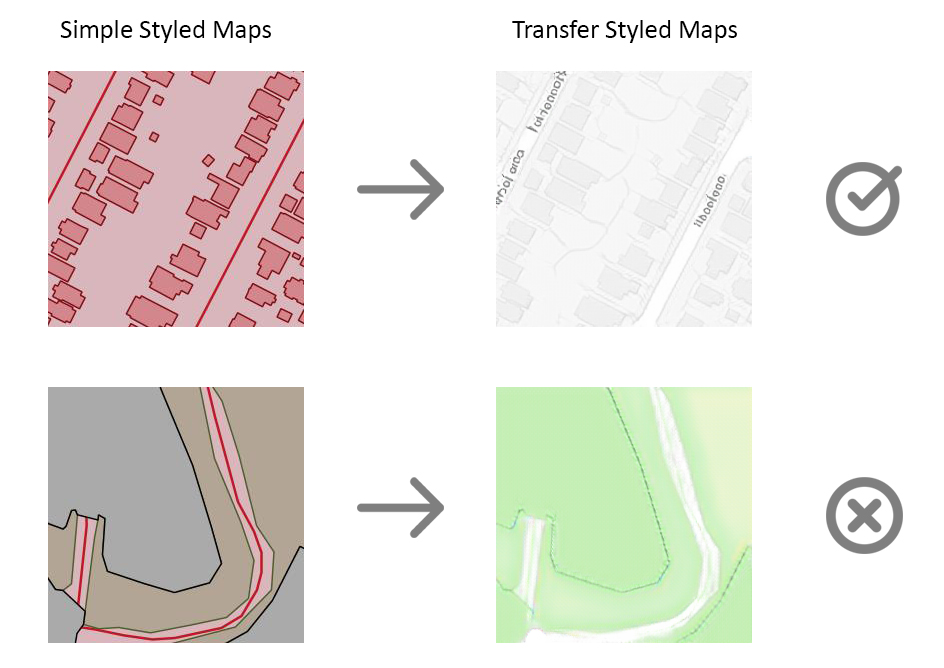
Figure 14: Examples of binary classification results of IsMap classifier. The transfer styled maps in above figure is classified as map correctly while in bottom is wrongly classified as photo.

Model	Pix2Pix		CycleGAN
Data	Level 15	Level 18	Level 15	Level 18
Precision	1.000	0.989	1.000	0.992
Recall	0.995	0.732	1.000	0.911
Accuracy	0.998	0.862	1.000	0.951
F1-Score	0.998	0.841	1.000	0.950

Table 1: Evaluation metrics of two GAN models at different map zoom levels

4 Discussion

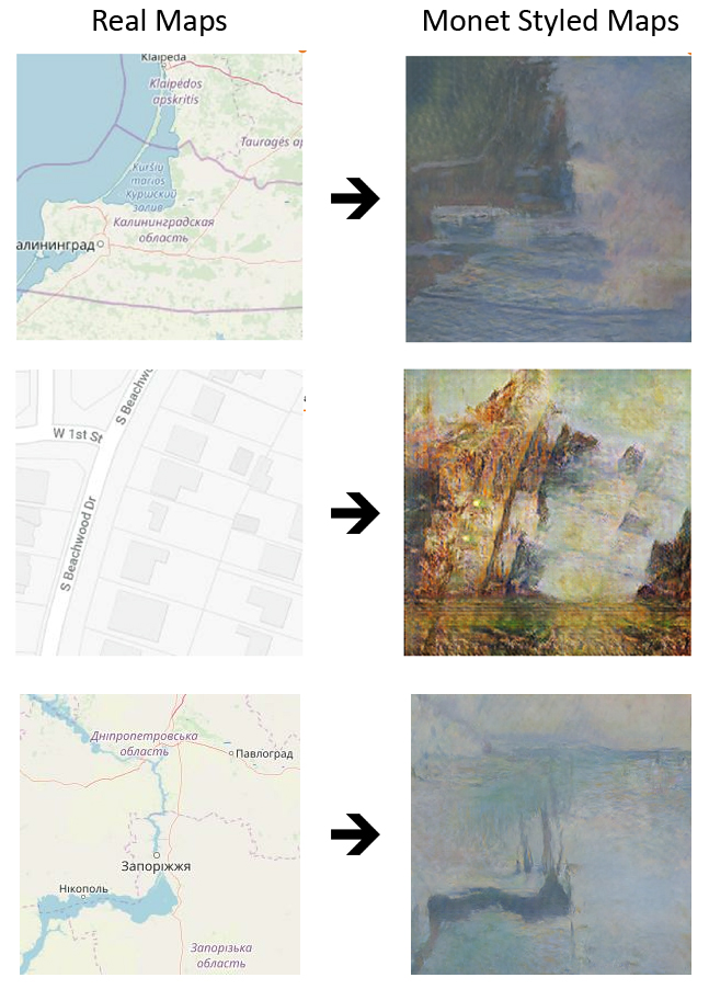
Figure 15: Results with transferred Monet painting styles using CycleGAN. The left column is real OSM maps, and the right column is the maps with Monet painting styles transferred. Results are not good.

The results of our experiments with the Google Maps style are encouraging, and generate several insights into future research at the intersections of AI and cartographic design. First, we explored if non-map input also might work for map style transfer using GANs. As an example, we downloaded an artwork library by Claude Monet—an impressionist painter with an aesthetic style characterized by vivid use of color and dramatic interplay of light and shadow—for use as a target painting style. Figure 3 shows several Monet examples used as the target painting style. While Monet primarily painted landscapes, there is no georeferenced information in the downloaded Monet artwork library and thus requires the unpaired CycleGAN model for style transfer. We again employed OSM for the simple styled maps receiving the target painting style. Figure 15 shows several transfer styled maps generated by CycleGAN using the Monet target style. Qualitatively, the output transfer styled maps appear to resemble paintings more than maps, although some map-like shapes and structures emerge. To confirm our visual interpretation, we again imported the Monet inspired transfer styled maps into the IsMap classifier and then used a modified deep-CNN classifier to categorize the images as photos, maps, or (new to the modified classifier) paintings. Less than 1$\%$ of the transfer styled maps are classified as maps, with most instead classified as paintings. One possible reason for the poorer results is less intensive training on the limited set of input visual art compared to the voluminous map tilesets. Therefore, transferring styles from visual art to maps might not be effective using the current workflow and requires further research.

Second, we took a deeper look at the way that the GANs generalize linework from the input simple styled maps in the resulting transfer style maps. Figure 16 shows how the GAN transfer effectively approximates several generalization operators (including enhancement, selection, and typify) to mimic the target Google Maps style at zoom level 15. First, enhancement of the road width is applied to create an artificial road hierarchy present across the target styled maps but not included in the original simple styled maps (Figure 16, top). Based on our analysis, the distance from buildings to roads is the primary spatial structure that affects how the GANs apply the enhanced road weight. Second, many roads are selectively eliminated from the simple styled maps in the resulting zoom level 15 transfer styled maps (Figure 16, middle). Roads that do not follow the orientation of the general street network are more likely candidates for elimination, such as the circled road running southeast to northwest. Finally, point markers are typified in the transfer styled maps, with the marker placed in the general location of a number of representative points of interest (POIs) from the simple styled maps (Figure 16, bottom). It is important to note that the GAN models are unlikely applying specific rule-based generalization operators, but rather the resulting transfer styled maps exhibit characteristics of these operators. Studying the generalization operators approximated by GANs may help optimize manual generalization and provide new insights for cartographic design broadly.

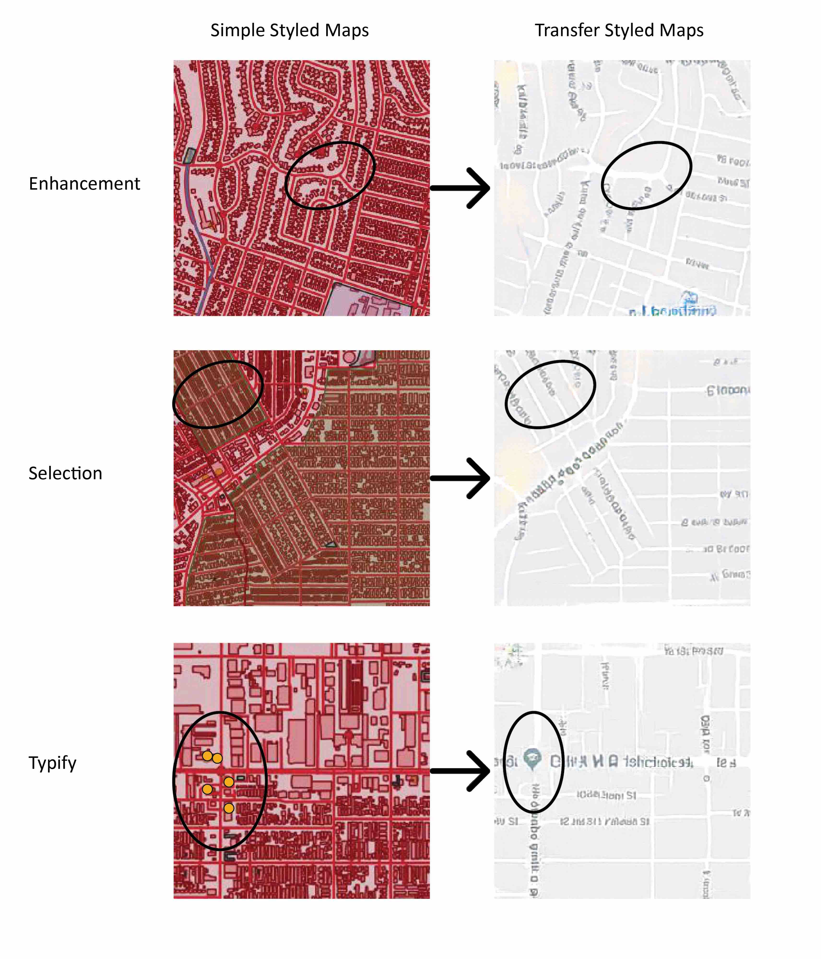
Figure 16: Examples of map generalization. The first row shows enhancement as the road in the black circle thickened; the second row shows selection as the road in the black circle is not selected in the transfer styled maps; the last row shows typify as several POIs are represented as one marker.

Finally, most existing research about map styling is based on vector data. Vector data records spatial coordinates and feature attributes separately, making it convenient and suitable for geometry generalization and symbol styling. However, our research is based on raster data, as GANs more commonly are used to process images. Each approach has pros and cons. Different map features are stored in different layers of vector data, meaning the styling of each layer is independent from others. As a result, styling of different layers may not work in concert in some places, making it difficult to achieve an optimal set of styles that work cohesively across the ‘map of everywhere’. Additionally, rich vector data requires more computing resources to apply the styles, limiting both design exploration by the cartographer and real-time rendering for the audience. In comparison, raster data—such as the tilesets used in this research—collapse both the spatial and attribute information into a single pixel value. With advanced image processing methods like convolutional neural networks and GANs, it is easier to calculate the output styling for raster tilesets, enabling large volume style transfer without complex style lists. However, the topology relationship of spatial features may break because such raster-based methods only use the single pixel value for computation. For example, Figure 17 shows one common topology error occurring in our research: road intersections. In the transferred styled maps, the bold roads pass one over another rather than intersect, while in the target styled maps, roads are connected via the intersection. In the future, we plan on exploring techniques to minimize topology errors in the transfer styled maps.

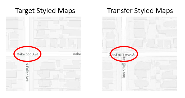
Figure 17: Example of a topology error in this study. Compared with the target styled maps, the topology of the road intersection in the transfer styled maps is wrong.

5 Conclusion and Future Work

In this research, we investigate multiscale map style transfer using state-of-the-art AI techniques. Specifically, two conditional generative adversarial network models, the Pix2Pix based on paired data and the CycleGAN based on unpaired data, are employed for the cartographic style transfer. The results of two methods show that GANs have the capability to transfer styles from customized styled maps like Google Maps to another without CartoCSS style sheets.

To answer the three research questions proposed in section 1, the study explored whether the two models can preserve both the complex patterns of spatial features and the aesthetic styles in generated maps. From the qualitative visual analysis, several visual variables of the target styled maps are retained, including the feature color, the line width (size), and feature shape, especially in urban areas with buildings and roads. The locations of some markers and annotations are also learned from the transfer styled maps. However, the GANs failed to apply legible text labels from the target styled maps. Moreover, we tested the performance of two models at two different zoom levels of the map data with different geographic ranges and feature compositions. In order to check whether the output still appears to be maps, we implemented a deep convolutional neural network to evaluate the results.

The CycleGAN model performs better than the Pix2Pix model using quantitative measures in our experiments regardless of the map zoom level. The transfer styled maps at level 15 perform better than that at level 18 using both Pix2Pix and CycleGAN models. There is a wide gap in performance at zoom level 18, with CycleGAN producing an F1-score of 0.95 but Pix2Pix only reaching a score of 0.841. Thus, geographic features at small scales can be generalized automatically, and important result with positive implications for the use of AI to assist with multiscale generalization and styling. Taken together, these findings prove that GANs have a great potential for map style rendering, transferring, and maybe other tasks in cartography.

Although most generated maps look realistic, several problems and challenges remain. First, since the GAN models are based on pixels from the input images, the topology of geographic features may not be well retained as discussed in Section 4. Second, because of the existence of point markers and textual labels in the tiled maps, the quality of transfer styled maps are influenced by them. However, the markers and text labels are important to the map purpose and might require separate pattern recognition models (Chiang,, 2016) to achieve better results. Therefore, in our future work, we also plan to train maps without labels and markers to reduce the bias caused by them.

In sum, this research demonstrates substantial potential for implementing artificial intelligence techniques in cartography. We outline several important directions for the use of AI in cartography moving forward. First, our use of GANs can be extended to other mapping contexts to help cartographers deconstruct the most salient stylistic elements that constitute the unique look and feel of existing designs, using this information to improve designs in future iterations. This research also can help non-experts who lack professional cartographic knowledge and experience to generate reasonable cartographic style sheet templates based on inspiration maps or visual art. Finally, integration of AI with cartographic design may automate part of the generalization process, a particularly promising avenue given the difficult of updating high resolution datasets and rendering new tilesets to support the ’map of everywhere’.

References

- Armstrong and Xiao, (2018) Armstrong, M. P. and Xiao, N., 2018. Retrospective deconstruction of statistical maps: A choropleth case study. Annals of the American Association of Geographers 108(1), pp. 179–203.