Abstract

This article is concerned with the approximation and expressive powers of deep neural networks. This is an active research area currently producing many interesting papers. The results most commonly found in the literature prove that neural networks approximate functions with classical smoothness to the same accuracy as classical linear methods of approximation, e.g. approximation by polynomials or by piecewise polynomials on prescribed partitions. However, approximation by neural networks depending on $n$ parameters is a form of nonlinear approximation and as such should be compared with other nonlinear methods such as variable knot splines or $n$-term approximation from dictionaries.

The performance of neural networks in targeted applications such as machine learning indicate that they actually possess even greater approximation power than these traditional methods of nonlinear approximation. The main results of this article prove that this is indeed the case. This is done by exhibiting large classes of functions which can be efficiently captured by neural networks where classical nonlinear methods fall short of the task.

The present article purposefully limits itself to studying the approximation of univariate functions by ReLU networks. Many generalizations to functions of several variables and other activation functions can be envisioned. However, even in this simplest of settings considered here, a theory that completely quantifies the approximation power of neural networks is still lacking.

AMS subject classification: 41A25, 41A30, 41A46, 68T99, 82C32, 92B20
Key Words: neural networks, rectified linear unit (ReLU), expressiveness, approximation power

1 Introduction

Neural networks produce structured parametric families of functions that have been studied and used for almost 70 years, going back to the work of Hebb in the late 1940’s [14] and of Rosenblatt in the 1950’s [24]. In the last several years, however, their popularity has surged as they have achieved state-of-the-art performance in a striking variety of machine learning problems, from computer vision [17] (e.g. self-driving cars) to natural language processing [30] (e.g. Google Translate) and to reinforcement learning (e.g. superhuman performance at Go [27, 28]). Despite these empirical successes, even their proponents agree that neural networks are not yet well-understood and that a rigorous theory of how and why they work could lead to significant practical improvements [3, 19].

An often cited theoretical feature of neural networks is that they produce universal function approximators [5, 16] in the sense that, given any continuous target function $f$ and a target accuracy $\epsilon>0$, neural networks with enough judiciously chosen parameters give an approximation to $f$ within an error of size $\epsilon$. Their universal approximation capacity has been known since the $1980$’s, yet it is not the main reason why neural networks are so effective in practice. Indeed, many other families of functions are universal function approximators. For example, one can approximate a fixed univariate real-valued continuous target function $f:[0,1]\rightarrow\mathbb{R}$ using Fourier expansions, wavelets, orthogonal polynomials, etc. [11]. All of these approximation methods are universal. Not only that, but in these more traditional settings, through the core results of Approximation Theory [11, 8], we have a complete understanding of the properties of the target function $f$ which determine how well it can be approximated given a budget for the number of parameters to be used. Such characterizations do not exist for neural network approximation, even in the simplest setting when the target function is univariate and the network’s activation function is the Rectified Linear Unit ($\mathrm{ReLU}$).

The neural networks used in modern machine learning are distinguished from those popular in the $1980$’s$/90$’s by an emphasis on using deep networks (as opposed to shallow networks with one hidden layer). If the universal approximation property were key to the impressive recent successes of neural networks, then the depth of the network would not matter since both shallow and deep networks are universal function approximators.

The present article focuses on the advantages of deep versus shallow architectures in neural networks. Our goal is to put mathematical rigor into the empirical observation that deep networks can approximate many interesting functions more efficiently, per parameter, than shallow networks (see [15, 29, 31, 32] for a selection of rigorous results).

In recent years, there has been a number of interesting papers that address the approximation properties of deep neural networks. Most of them treat ReLU networks since the rectified linear unit is the activation function of preference in many applications, particularly for problems in computer vision. Let us mention, as a short list, some papers most related to our work. It is shown in [12] that deep ReLU networks can approximate functions of $d$ variables as well as linear approximation by algebraic polynomials with a comparable number of parameters. This is done by using the fact (proved by Yarotsky [31]) that power functions $x^{\nu}$ can be approximated with exponential efficiency by deep ReLU networks. Yarotsky also showed that certain classes of classical smoothness (Lipschitz spaces) can be approximated with rates slightly better than that of classical linear methods (see [32]). The main advantage of deep neural networks is that they can output compositions of functions cheaply. This fact has been exploited by many authors (see e.g. [23], where this approach is formalized, and [2] where this property is used to compare deep network approximation with nonlinear shearlet approximation).

In the present paper, we address the approximation power of $\mathrm{ReLU}$ networks and, in particular, whether such networks are truly more powerful in approximation efficiency than the classical methods of approximation. Although most of our results generalize to the approximation of multivariate functions, we discuss only the univariate setting since this gives us the best chance for definitive results. Our main focus is on the advantages of depth, i.e., what advantages are present in deep networks that do not appear in shallow networks. We restrict ourselves to ReLU networks since they have the simplest structure and should be easiest to understand.

We emphasize that, when discussing approximation efficiency, we assume that $f$ is fully accessible and we ask how well $f$ can be approximated by a neural network with $n$ parameters. This is in contrast to problems of data fitting where, instead of full access to $f$, we only have some data observations about it. In the latter case, the approximation can only use the given data and its performance would depend on the amount and form of that data. Performance in data fitting is often formulated in a stochastic setting in which it is assumed that the data is randomly generated and both the observations and the gradient descent parameter updates are noisy. The data fitting problem, using a specific form of approximation like neural networks, has two components, commonly referred to as bias and variance. We are concentrating on the bias component. It plays a fundamental role not only in data fitting but also in any numerical procedures based on neural network approximation.

Given two integers $W\geq 2$ and $L\geq 1$, we let (precise definitions are given in the next section)

$$\Upsilon^{W,L}:=\{S:\mathbb{R}\rightarrow\mathbb{R},\,\,S\text{ \ is produced by a }\mathrm{ReLU}\text{ network of width }W\text{ and depth }L\},$$ (1)

and denote by $n(W,L)$ the number of its parameters. We fix $W$ and study the approximation families $\Upsilon^{W,L}$ when the number of layers $L$ is allowed to vary. Our interest is in understanding why taking $L$ large, i.e., why using deep networks is beneficial. One way to investigate the approximation power of $\Upsilon^{W,L}$ is to first compare it to known nonlinear approximation families with essentially the same number of degrees of freedom. Since every element in $\Upsilon^{W,L}$ is a Continuous Piecewise Linear (CPwL) function, the classical approximation family closest to $\Upsilon^{W,L}$ is the nonlinear set

$$\Sigma_{n}:=\{S:\mathbb{R}\rightarrow\mathbb{R},\,\,S\text{ is a CPwL function with at most }n\text{ distinct breakpoints in }(0,1)\}.$$

The elements of $\Sigma_{n}$ are also called free knot linear splines. We place the restriction that the breakpoints are in $(0,1)$ because we are concerned with approximation on the interval $[0,1]$.

When $n\asymp n(W,L)$, the sets $\Sigma_{n}$ and $\Upsilon^{W,L}$ have comparable complexity in terms of parameters needed to describe them, since the elements in $\Sigma_{n}$ are determined by $2n+2$ parameters. This comparison also probes the expressive power of depth for $\mathrm{ReLU}$ networks because $\Sigma_{W}$ is (essentially) the same as the one-layer $\mathrm{ReLU}$ network $\Upsilon^{W,1}$, see (4).

Several interesting results [6, 21, 29] show that, for arbitrarily large $k\geq 1$ and $n=n(W,L)$ sufficiently large,

$$\Upsilon^{W,L}\setminus\Sigma_{{n}^{k}}\neq\emptyset,$$ (2)

cf e.g. [29, Theorem 1.2]. This means that sufficiently deep $\mathrm{ReLU}$ networks with $n$ parameters can compute certain CPwL functions whose number of breakpoints exceeds any power of $n$ (the increase of the network depth is necessary as $k$ grows). The reason for (2) is that composing two CPwL functions can multiply the number of breakpoints, allowing networks with $L$ layers of width $W$ to create roughly $W^{L}$ breakpoints for very special choices of weights and biases. By choosing to use the available $n$ parameters in a deep rather than shallow network, one can thus produce functions with many more breakpoints than parameters, albeit these functions have a very special structure.

The first natural question to answer in comparing $\Sigma_{n}$ with $\Upsilon^{W,L}$ is whether, for every fixed $W\geq 2$, each function $S\in\Sigma_{n}$ is in a corresponding set $\Upsilon^{W,L}$ with $n(W,L)\asymp n$, i.e., with a comparable number of parameters. This would guarantee we do not lose anything in terms of expressive power when considering deep networks with fixed width $W$ over shallow networks with fixed depth $L$. One of our results, Theorem 3.1, gives a resolution to this question and shows that, up to a constant multiplicative factor, fixed-width $\mathrm{ReLU}$ networks depending on $n$ parameters are at least as expressive as the free knot linear splines $\Sigma_{n}$. In other words, deep ReLU networks retain all of the approximation power of free knot linear splines but also add something since they can create functions which are far from being in $\Sigma_{n}$. We want to understand the new functions being created and how they can assist us in approximation and thus in data fitting. In this direction, we showcase in §5 and §6 two classes of functions easily produced by $\mathrm{ReLU}$ networks, one consisting of self-similar functions and the other emulating trigonometric functions. Appending these classes to $\Sigma_{n}$ naturally provides a powerful dictionary for nonlinear approximation.

What types of results could effectively explain the increased approximation power of deep networks as compared with other forms of approximation? One possibility is to exhibit classes $K$ of functions on which the decay rate of approximation error for neural networks is better than for other methods (linear or nonlinear) while depending on the same number of parameters. On this point, let us mention that by now there are several theorems in the literature (see e.g. [2, 4, 22, 26]) which show that neural networks perform as well as certain classical methods such as polynomials, wavelets, shearlets, etc., but they do not show that neural networks perform any better than these methods.

We seek more convincing results providing compact classes $K$ that are subsets of Banach spaces $X$ on which neural networks perform significantly better than other methods of approximation. In this direction, we mention at the outset that such sets $K$ cannot be described by classical smoothness (such as Lipschitz, Sobolev, or Besov regularity) because for classical smoothness classes $K$, there are known lower bounds on the performance for any methods of approximation (linear or nonlinear). These lower bounds are provided by concepts such as entropy and widths. However, let us point out that there is an interesting little twist here that allows deep neural networks to give a slight improvement over classical approximation methods for certain Lipschitz, Sobolev, and Besov classes (see Theorems 7.3 and 7.4). This improvement is possible when the selection of parameters used in the approximation is allowed to be unstable.

Our results on the expressive power of depth describe certain classes of functions that can be approximated significantly better by $\Upsilon^{W,L}$ than by $\Sigma_{n}$ when $n(W,L)$ is comparable to $n$, see §7.3. The construction of these new classes of functions exploits the fact that, when $S$ and $T$ are functions in $\Sigma_{n}$, their composition $S\circ T$, can be produced by fixed-width $\mathrm{ReLU}$ networks depending on a number of parameters comparable to $n$, This composition property allows one to construct broad classes of functions, based on self similarity, whose approximation error decays exponentially using deep networks but only polynomially using $\Sigma_{n}$ (due to the utter failure of this composition property for $\Sigma_{n}$).

2 Preliminaries and notation

To set some notation, recall the definition of the ReLU function applied to $x=(x_{1},\dots,x_{d})\in\mathbb{R}^{d}$:

$$\mathrm{ReLU}(x_{1},\ldots,x_{d})=(\mathrm{ReLU}(x_{1}),\ldots,\mathrm{ReLU}(x_{d}))=(\max\left\{0,x_{1}\right\},\ldots,\max\left\{0,x_{d}\right\}).$$

Definition 2.1.

A fully connected feed-forward $\mathrm{ReLU}$ network ${\cal N}$ with width $W$ and depth $L$ is a collection of weight matrices $M^{(0)},\dots,$ $M^{(L)}$ and bias vectors $b^{(0)},\dots,b^{(L)}$. The matrices $M^{(\ell)}$, $\ell=1,\ldots,L-1$, are of size $W\times W$, whereas $M^{(0)}$ has size $W\times 1$, and $M^{(L)}$ has size $1\times W$. The biases $b^{(\ell)}$ are vectors of size $W$ if $\ell=0,\dots,L-1$ and a scalar if $\ell=L$. Each such network ${\cal N}$ produces a univariate real-valued function

$$A^{(L)}\circ\mathrm{ReLU}\circ A^{(L-1)}\circ\cdots\circ\mathrm{ReLU}\circ A^{(0)}(x),\quad x\in\mathbb{R},$$

where

$$A^{(\ell)}(y)=M^{(\ell)}y+b^{(\ell)},\quad\ell=0,\dots,L.$$

We define $\Upsilon^{W,L}$ as the set of such functions resulting from all possible choices of weights and biases.

Every $S\in\Upsilon^{W,L}$ is a CPwL function on the whole real line. For each input $x:=x^{(0)}\in\mathbb{R}$, the value $S(x^{(0)})$ of any $S\in\Upsilon^{W,L}$ is computed after the calculation of a series of intermediate vectors $x^{(\ell)}\in\mathbb{R}^{W}$, called vectors of activation at layer $\ell$, $\ell=1,\ldots,L$, before finally producing the output $x^{(L+1)}=M^{(L)}x^{(L)}+b^{(L)}$. The computations performed by such a network to produce an $S\in\Upsilon^{W,L}$ are shown schematically in Figure 1.

Figure 1: The computation graph associated to a neural network with input/output dimension $1$, width $W=3$ and $L$ hidden layers. The edges between layers $\ell-1$ and $\ell$ are labeled by the entries of the weight matrix $M^{(\ell-1)}$. The $j^{th}$ node (called a neuron) at layer $\ell$ computes the $j^{th}$ component of $x^{(\ell)}$ by taking the dot product of the $j^{th}$ row of $M^{(\ell-1)}$ with the entries of $x^{(\ell-1)}$ and adding it to the $j^{th}$ entry of the vector $b^{(\ell-1)}$ of biases.

For example, the hat function (also called triangle function) $H:[0,1]\rightarrow\mathbb{R}$, defined as

$$H(x)=2(x-0)_{+}-4\Big{(}x-\frac{1}{2}\Big{)}_{+}=\begin{bmatrix}2&-4\end{bmatrix}\mathrm{ReLU}\left\{\begin{bmatrix}1\\ 1\end{bmatrix}x+\begin{bmatrix}0\\ -\frac{1}{2}\end{bmatrix}\right\}=\begin{cases}2x,\quad 0\leq x\leq\frac{1}{2},\\ 2(1-x),\,\,\frac{1}{2}<x\leq 1,\end{cases}$$ (3)

belongs to $\Upsilon^{2,1}$, see Figure 2.

Figure 2: The computation graph and usual graph associated to $H$.

For $L=1$, each function in $\Upsilon^{W,1}$ is a CPwL function with at most $W$ breakpoints determined by the nodes in the first layer. Conversely, any CPwL function with $(W-1)$ breakpoints interior to $[0,1]$, when considered on the interval $[0,1]$, is the restriction of a function from $\Upsilon^{W,1}$ to that interval. Indeed, the elements ${\mathcal{S}}\in\Sigma_{W-1}$ on $[0,1]$ can be represented as

$$ax+b+\sum_{j=1}^{W-1}m_{j}(x-\xi_{j})_{+}=\begin{bmatrix}a&m_{1}&\ldots&m_{W-1}\end{bmatrix}\mathrm{ReLU}\left\{\begin{bmatrix}1\\ 1\\ \ldots\\ 1\end{bmatrix}x+\begin{bmatrix}0\\ -\xi_{1}\\ \ldots\\ -\xi_{W-1}\end{bmatrix}\right\}+b,$$

where $\xi_{1},\ldots,\xi_{W-1}$ are the interior breakpoints. In other words, as functions on $[0,1]$, we have

$$\Sigma_{W-1}\subset\Upsilon^{W,1}\subset\Sigma_{W},$$ (4)

which means that, for large $W$, the sets $\Upsilon^{W,1}$ and $\Sigma_{W}$ are essentially the same. Therefore, neural networks with one hidden layer have the same approximation power as CPwL functions with the same number of parameters.

The number of parameters used to generate functions in $\Upsilon^{W,L}$ is

$$n(W,L)~{}=~{}W(W+1)L-(W-1)^{2}+2.$$ (5)

Not all counted parameters (the weights, i.e., entries of $M^{(\ell)}$, and biases, i.e., entries of $b^{(\ell)}$) are independent, since for instance some of the multipliers used in the transition $x^{(L)}\rightarrow x^{(L+1)}$ could have been absorbed in the preceding layer. We write

$$n(W,L)\asymp W^{2}L$$

to indicate that $n(W,L)$ is comparable to $W^{2}L$, in the sense that there are constants $c,C>0$ such that $c\ W^{2}L\leq n(W,L)\leq C\ W^{2}L$ — one could take $c=1/2$ and $C=2$ when $W\geq 2$ and $L\geq 2$.

3 ReLU networks are at least as expressive as free knot linear splines

In this section, we fix $W\geq 4,L\geq 2$, and consider the set $\Upsilon^{W,L}$ defined in (1). Our goal is to prove that $\Sigma_{n}\subset\Upsilon^{W,L}$, where the number of its parameters $n(W,L)\leq Cn$ for a certain fixed constant $C$. In order to formulate our exact result we define $q:=\lfloor\frac{W-2}{6}\rfloor$ when $W\geq 8$ and $q:=2$ for $4\leq W<7$.

Theorem 3.1.

Fix a width $W\geq 4$. For every $n\geq 1$, the set $\Sigma_{n}$ of free knot linear splines with $n$ breakpoints is contained in the set $\Upsilon^{W,L}$ of functions produced by width-$W$ and depth-$L$ ReLU networks, where

$$L=\begin{cases}2\left\lceil\frac{n}{q(W-2)}\right\rceil,\quad&n\geq q(W-2),\\ 2,&n<q(W-2),\end{cases}$$

$$n(W,L)\leq\begin{cases}Cn,\quad&n\geq q(W-2),\\ W^{2}+4W+1,&n<q(W-2),\end{cases}$$

with $C$ an absolute constant.

Before giving the proof of Theorem 3.1 in §3.2 below we first introduce in §3.1 some notation.

3.1 Special $\mathrm{ReLU}$ neural networks

Our main vehicle for proving Theorem 3.1 is a special subset $\overline{\underline{\Upsilon}}^{W,L}\subset\Upsilon^{W,L}$, which we now describe. Given a width $W\geq 4$ and a depth $L\geq 2$, we focus on networks where a special role is reserved for two nodes in each hidden layer, see Figure 3, which depicts these nodes as the first (“top”) and at the last (“bottom”) node of each hidden layer, respectively.

Figure 3: The computation graph associated to $\overline{\underline{\Upsilon}}^{5,6}$.

The top neuron (first node), which is $\mathrm{ReLU}$ free, is used to simply copy the input $x$. The concatenation of all these top nodes can be viewed as a special “channel” (a term borrowed from the electrical engineering filter-bank literature) that skips computation altogether and just carries $x$ forward. We call this the source channel (SC). The bottom neuron (last node) in each layer, which is also $\mathrm{ReLU}$ free, is used to collect intermediate results. We call the concatenation of all these bottom nodes the collation channel (CC). This channel never feeds forward into subsequent calculations, it only accepts previous calculations. The rest of the channels are computational channels (CmC). The fact that a special role is reserved for two channels enforces the natural restriction $W\geq 4$, since we need at least two computational channels. We call these networks (with SC and CC) special neural networks, for which we introduce a special notation, featuring a top and a bottom horizontal line to represent the SC and CC, respectively. Namely, we set

$$\overline{\underline{\Upsilon}}^{W,L}=\{S:[0,1]\rightarrow\mathbb{R},\,\,S\text{ \ is produced by a special network of width }W\text{ and depth }L\}.$$

We feel that these more structured networks are not only useful in proving results on approximation but may be useful in applications such as data fitting. In practice, the designation of the first row as a SC and the last row as a CC amounts to having matrices $M^{(\ell)}$ and vectors $b^{(\ell)}$ of the form

$$M^{(0)}=\begin{bmatrix}1&m_{2}^{(0)}&\ldots&m_{W-1}^{(0)}&0\end{bmatrix}^{\top},\quad b^{(0)}=\begin{bmatrix}0&b_{2}^{(0)}&\ldots&b_{W-1}^{(0)}&0\end{bmatrix}^{\top},$$

$$M^{\ell)}=\begin{bmatrix}1&0&\ldots&0&0\\ m_{2,1}^{(\ell)}&m_{2,2}^{(\ell)}&\ldots&m_{2,W-1}^{(\ell)}&0\\ m_{3,1}^{(\ell)}&m_{3,2}^{(\ell)}&\ldots&m_{3,W-1}^{(\ell)}&0\\ \ldots&\ldots&\\ m_{W-1,1}^{(\ell)}&m_{W-1,2}^{(\ell)}&\ldots&m_{W-1,W-1}^{(\ell)}&0\\ m_{W,1}^{(\ell)}&m_{W,2}^{(\ell)}&\ldots&m_{W,W-1}^{(\ell)}&1\end{bmatrix},\quad b^{(\ell)}=\begin{bmatrix}0\\ b_{2}^{(\ell)}\\ b_{3}^{(\ell)}\\ \ldots\\ b_{W-1}^{(\ell)}\\ b_{W}^{(\ell)}\end{bmatrix},\quad\ell=1,\ldots,L-1,$$ (6)

and

$$M^{(L)}=\begin{bmatrix}m_{1}^{(L)}&\ldots&m_{W-1}^{(L)}&1\end{bmatrix},\quad b^{(L)}\in\mathbb{R}.$$

Remark 3.1.

Note that since the SC and CC are ReLU-free, the width-$W$ depth-$L$ special networks do not form a subset of the set of width-$W$ depth-$L$ ReLU networks. However, in terms of sets of functions produced by these networks, the inclusion

$$\overline{\underline{\Upsilon}}^{W,L}\subset\Upsilon^{W,L}$$ (7)

is valid. Indeed, given $\bar{S}\in\overline{\underline{\Upsilon}}^{W,L}$, determined by the set of matrices and vectors $\{\bar{M}^{(\ell)},\bar{b}^{(\ell)}\}$, $\ell=0,\ldots,L$, we will construct $\{M^{(\ell)},b^{(\ell)}\}$, $\ell=0,\ldots,L$, such that $\bar{S}$ is also the output of a $\mathrm{ReLU}$ network with the latter matrices and vectors. First, notice that the input $x\in[0,1]$, and therefore we have $x=\mathrm{ReLU}(x)$. Next, since the bottom neuron in the $\ell$-th layer, $\ell=1,\ldots,L$, collects a function $\bar{S}^{(\ell)}(x)$ depending continuously on $x\in[0,1]$, there is a constant $C_{\ell}$ such that $\bar{S}^{(\ell)}(x)+C_{\ell}\geq 0$ for all $x\in[0,1]$. Hence $\bar{S}^{(\ell)}(x)=\mathrm{ReLU}(\bar{S}^{(\ell)}(x)+C_{\ell})-C_{\ell}$. Therefore, the $\mathrm{ReLU}$ network that produces $\bar{S}$ has the same matrices $M^{(\ell)}=\bar{M}^{(\ell)}$ and vectors $b^{(\ell)}$, $\ell=1,\ldots,L-1$, where

$$b^{(\ell)}_{j}=\bar{b}^{(\ell)}_{j},\quad j=1,\ldots,W-1,\quad b^{(\ell)}_{W}=\bar{b}^{(\ell)}_{W}+C_{\ell},$$

and $b^{(L)}=\bar{b}^{(L)}-\sum_{\ell=1}^{L-1}C_{\ell}$.

Proposition 3.2.

Special $\mathrm{ReLU}$ neural networks produce sets of CPwL functions that satisfy the following properties:
(i) For all $W,L,Q$,

$$\overline{\underline{\Upsilon}}^{W,L}+\overline{\underline{\Upsilon}}^{W,Q}\subset\overline{\underline{\Upsilon}}^{W,L+Q}.$$ (8)

(ii) For $L<P$,

$$\overline{\underline{\Upsilon}}^{W,L}\subset\overline{\underline{\Upsilon}}^{W,P}.$$

Proof: To show (i), we first fix $S\in\overline{\underline{\Upsilon}}^{W,L}$ and $T\in\overline{\underline{\Upsilon}}^{W,Q}$ and use the following ‘concatenation’  of the special networks for $S$ and $T$. The concatenated network has the same input and first $L$ hidden layers as the network that produced $S$. Its $(L+1)$-st layer is the same as the first hidden layer of the network that produced $T$ except that in the collation channel it places $S$ rather than $0$. The remainder of the concatenated network is the same as the remaining layers of the network producing $T$ except that the collation channel is updated, see Figure 4. The proof of (ii) follows the proof of (i) with $Q=P-L$ and $T\equiv 0$. $\Box$

Figure 4: The computational graph for summation.

3.2 Proof of Theorem 3.1

In this section, we prove Theorem 3.1. Namely, we show that for any fixed width $W\geq 4$, any element $T$ in $\Sigma_{n}$ is the output of a special network with a number of parameters comparable to $n$.

Our constructive proof begins with Lemma 3.3, in which we create a special $\mathrm{ReLU}$ network with only $2$ layers that generates a particular collection of CPwL functions, see (9). To describe this collection, we consider any positive integer $N$ of the form $N:={q(W-2)}$, where $q:=\lfloor(W-2)/6\rfloor$. Since it is meaningful to have only cases when $q\geq 1$, we impose the restriction $W\geq 8$. In the Appendix, we treat the remaining cases when $4\leq W<8$. Notice that $N$ is small and so at this stage we are only showing how to construct CPwL functions with a few breakpoints.

Let $x_{1}<\cdots<x_{N}\in(0,1)$ be any $N$ given breakpoints in $(0,1)$ and choose $x_{0}$ and $x_{N+1}$ to be any two additional points such that $0\leq x_{0}<x_{1}$ and $1\geq x_{N+1}>x_{N}$. The set of all CPwL functions which vanish outside of $[x_{0},x_{N+1}]$ and have breakpoints only at the $x_{0},x_{1},\dots,,x_{N},x_{N+1}$ is denoted by

$${\cal S}:={\cal S}(x_{0},\dots,x_{N+1})$$ (9)

and is a linear space of dimension $N$. We create a basis for ${\cal S}$ the following way. We denote by $\xi_{j}$, $j=1,\dots,(W-2)$, the points $\xi_{j}:=x_{jq}$, which we call principal breakpoints and to each principal breakpoint $\xi_{j}$, we associate $q$ basis functions $H_{i,j}$, $i=1,\dots,q$. Here $H_{i,j}$, see Figure 5,

Figure 5: The graphs of $H_{i,j}$.

is a hat function supported on $I_{i,j}:=[x_{jq-i,},x_{jq+1}]$ which takes the value $0$ at the endpoints of this interval, the value one at $\xi_{j}$ and is linear on each of the two intervals $[x_{jq-i,},x_{jq}]$ and $[x_{jq},x_{jq+1}]$, that is

$$H_{i,j}(x) = \begin{cases}\frac{x-x_{jq-i}}{x_{jq}-x_{jq-i}},&\mbox{ if }x\in(x_{jq-i},x_{jq}),\\ 0,&\mbox{ if}\ x\notin I_{i,j},\\ \frac{x-x_{jq+1}}{x_{jq}-x_{jq+1}},&\mbox{ if }x\in(x_{jq},x_{jq+1}).\end{cases}$$

We rename these hat functions as $\phi_{k}$, $k=1,\dots,N$, and order them in such a way that $\phi_{k}$ has leftmost breakpoint $x_{k-1}$. We say $\phi_{k}$ is associated with $\xi_{j}$ if $\xi_{j}$ is the principal breakpoint where it is nonzero. We claim that these $\phi_{k}$’s are a basis for ${\cal S}$. Indeed, since there are $N$ of them, we need only check that they are linearly independent. If $\sum_{k=1}^{N}c_{k}\phi_{k}=0$, then $c_{1}=0$ because $\phi_{1}$ is the only one of these functions which is nonzero on $[x_{0},x_{1}]$. We then move from left to right getting that each coefficient $c_{k}$ is zero.

Lemma 3.3.

For any $N$ breakpoints $x_{1}<\cdots<x_{N}\in(0,1)$, $N:={q(W-2)}$, $q:=\lfloor(W-2)/6\rfloor$, $W\geq 8$, ${\cal S}(x_{0},\dots,x_{N+1})\subset\overline{\underline{\Upsilon}}^{W,2}$.

Proof: Consider $T\in{\cal S}(x_{0},\dots,x_{N+1})$, $T=\sum_{k=1}^{N}c_{k}\phi_{k}$, and determine its principal breakpoints $\xi_{1},\ldots,\xi_{W-2}$ (every $q$-th point from the sequence $(x_{1},x_{2},\ldots,x_{N})$ is a principal breakpoint). We next represent the set of indices $\Lambda=\{1,\dots,N\}$ as a disjoint union of $K\leq 6q\leq W-2$ sets $\Lambda_{i}$,

$$\Lambda=\cup_{i=1}^{K}\Lambda_{i},$$

where the $\Lambda_{i}$’s have the following two properties:

• for any $\Lambda^{\prime}\in\{\Lambda_{1},\dots,\Lambda_{K}\}$, all of the coefficients $c_{k}$ with $k\in\Lambda^{\prime}$ of $T$ have the same sign.

• if $k,k^{\prime}\in\Lambda^{\prime}$, then the principal breakpoints $\xi_{j}$ and $\xi_{j^{\prime}}$ associated to $\phi_{k},\phi_{k^{\prime}}$ respectively, satisfy the separation property $|j-j^{\prime}|\geq 3$.

We can find such a partition as follows. First, we divide $\Lambda=\Lambda_{+}\cup\Lambda_{-}$ where for each $i\in\Lambda_{+}$, we have $c_{i}\geq 0$ and for each $i\in\Lambda_{-}$, we have $c_{i}<0$. We then divide each of $\Lambda_{+}$ and $\Lambda_{-}$ into at most $3q$ sets having the desired separation property. If $K<W-2$, we set $\Lambda_{K+1}=\ldots=\Lambda_{W-2}=\emptyset$. It may also happen that some of the $\Lambda_{k}$’s, $k\leq K$, are empty. In all cases for which $\Lambda_{k}=\emptyset$, we set $T_{k}=0$, and write

$$T=\sum_{k=1}^{W-2}T_{k},\quad T_{k}:=\sum_{i\in\Lambda_{k}}c_{i}\phi_{i},\quad k=1,\dots,W-2.$$ (10)

Notice that the $\phi_{i}$, $i\in\Lambda_{k}\neq\emptyset$, have disjoint supports and so $c_{i}=T_{k}(\xi_{j})$ where $\xi_{j}$ is the principal breakpoint associated to $\phi_{i}$.

We next show that each of the $T_{k}$ corresponding to a nonempty $\Lambda_{k}$ is of the form $\pm[S_{k}(x)]_{+}$ for some linear combination $S_{k}$ of the $(x-\xi_{j})_{+}$. Fix $k$ and first consider the case where all of the $c_{i}$ in $\Lambda_{k}$ are nonnegative. We consider the CPwL function $S_{k}$ which takes the value $c_{i}$ at each principal breakpoint $\xi_{j}$ associated to an $i\in\Lambda_{k}$. At the remaining principal breakpoints, we assign negative values to the $S_{k}(\xi_{j})$’s. We choose these negative values so that for any $i\in\Lambda_{k}$, $S$ vanishes at the leftmost and rightmost breakpoints of all $\phi_{i}$ with $i\in\Lambda_{k}$. This is possible because of the separation property (see the appendix for a particular strategy for defining the $\Lambda_{k}$). It follows that $[S_{k}(x)]_{+}=T_{k}(x)$. A similar construction applies when all the coefficients in $\Lambda_{k}$ are negative. In this case, $T_{k}=-[S_{k}]_{+}$ for the constructed $S_{k}$. A typical $T_{k}$, which for the sake of simplicity we call $\tilde{T}$, and its decomposition is pictured in Figure 6, see §9.1.

Figure 6: A typical $\tilde{T}$ computed by a node in the second layer of $\overline{\underline{\Upsilon}}^{W,2}$.

We can now describe the $\mathrm{ReLU}$ network that generates $T$. Since it is special, we focus only the computational channels. The computational nodes in the first layer are $(x-\xi_{j})_{+}$, $j=1,\dots,W-2$, where the $\xi_{j}$’s are the principal breakpoints. The computational nodes in the second layer are equal to the $[S_{k}]_{+}$ or $0$. Because of (10), the target $T$ is the output of this network with output layer weights $\pm 1$ or $0$. $\Box$

Remark 3.2.

If we want to generate with the same special $\mathrm{ReLU}$ network all spaces ${\cal S}(x_{0},\ldots,x_{N_{0}+1})$ with $N_{0}<N$, we can artificially add $(N-N_{0})$ distinct points in the interval $(x_{N_{0}},x_{N_{0}+1})$ and view the elements in ${\cal S}(x_{0},\ldots,x_{N_{0}+1})$ as CPwL with $N$ breakpoints vanishing outside $[x_{0},x_{N_{0}+1}]$, even though the last $N-N_{0}+1$ points are not really a breakpoints, except possibly $x_{N_{0}+1}$.

Figure 7: The graphs of $S_{j}$, $j=0,\ldots,L-1$.

Our next lemma shows how to carve up the target function $T\in\Sigma_{n}$ with a (possibly) large number of breakpoints into “bitesize” pieces that are handled by Lemma 3.3.

Lemma 3.4.

If $T\in\Sigma_{N}$ is any CPwL function on $[0,1]$ with $N=q(W-2)L$, $q:=\lfloor\frac{W-2}{6}\rfloor$, $W\geq 8$, then $T$ is the output of a special $\mathrm{ReLU}$ network $\overline{\underline{\Upsilon}}^{W,2L}$ with at most $2L$ layers.

Proof: Let $x_{1}<\cdots<x_{N}$ be the breakpoints of $T$ in $(0,1)$ and set $x_{0}:=0,x_{N+1}:=1$. We define $\ell(x):=ax+b$ to be the linear function which interpolates $T$ at the endpoints $0,1$ and set $S:=T-\ell$. We can write $S=S_{0}+\dots+S_{L-1}$, where $S_{j}\in\Sigma_{N}$ is the CPwL function which agrees with $S$ at the points $x_{i}$, for all indices $i\in\{jq(W-2)+1,\dots,(j+1)q(W-2)\}$ and is zero at all other breakpoints of $T$, see Figure 7.

Clearly, see (9),

$$S_{j}\in{\cal S}(x_{jq(W-2)},\ldots,x_{(j+1)q(W-2)+1}),\quad j=0,\ldots,L-1,$$

and therefore, it follows from Lemma 3.3 that each $S_{j}\in\overline{\underline{\Upsilon}}_{j}^{W,2}$. We concatenate the $L$ networks that produce $S_{j}\in\overline{\underline{\Upsilon}}_{j}^{W,2}$, $j=0,\ldots,L-1$, as described in Proposition 3.2 and thereby produce $S$. In order to account for the linear term $\ell(x)$, we assign weight $a$ and bias $b$ to the output of the node of the skip channel in the last layer of the concatenated network, see Figure 8.

Figure 8: The resulting network with $2L$ layers.

$\Box$

Proof of Theorem 3.1: Now we are ready to complete the proof of Theorem 3.1.

Case 1: We first consider the case when $W\geq 8$. Lemma 3.4 and inclusion (7) show that $\Sigma_{N}\subset\Upsilon^{W,2L}$ with $N=q(W-2)L$ and $q:=\lfloor\frac{W-2}{6}\rfloor$. Given $n$, we choose $N$ as the smallest $N$ of the above form for which $n\leq N$, Let $N_{1}:=q(W-2)$. If $n\geq N_{1}$, we choose $L$ as

$$L~{}=~{}L(n,W)~{}:=~{}\left\lceil\frac{n}{q(W-2)}\right\rceil,$$

and thus $L<\frac{n}{q(W-2)}+1.$ Using (5), we have that the number of parameters in $\Upsilon^{W,2L}$ is

$$n(W,2L)<2W(W+1)\left(\frac{n}{q(W-2)}+1\right)-(W-1)^{2}+2=\frac{2W(W+1)}{q(W-2)}n+W^{2}+4W+1.$$

Optimizing over $W$ show that the maximum of $\frac{2W(W+1)}{q(W-2)}$ over integers $W\geq 8$ is achieved at $W=13$ and $q=1$, giving the value $\frac{364}{11}<34$. Hence,

$$n(W,2L)<34n+W^{2}+4W+1<34n+27q(W-2)\leq 61n,$$

where we used that $W/13\leq q$ and $q(W-2)=N_{1}\leq n$.

On the other hand if $n<N_{1}:=q(W-2)$, then Lemma 3.4 and inclusion (7) show that $\Sigma_{n}\subset\Sigma_{N_{1}}\subset\Upsilon^{W,2}$. Then, we have

$$n(W,2)=W^{2}+4W+1,$$

as desired.

Case 2: The proof of the case $4\leq W<7$ is discussed in the appendix.

$\Box$

Remark 3.3.

We have not tried to optimize constants in the above theorem. If one counts the actual number of parameters used in $\Upsilon^{W,L}$ (rather than the parameters available), one obtains a much better constant. We know, in fact, that we can present other constructions (different than those given here) which provide a better constant in the statement of Theorem 3.1.

4 More about standard and special networks

In this section, we discuss further properties of the sets $\Upsilon^{W,L}$ and $\overline{\underline{\Upsilon}}^{W,L}$. We highlight in particular Theorem 4.1, which is a generalization of Theorem 3.1, and whose proof is deferred to the appendix. Note that the conclusion of Theorem 3.1 depends on the ranges of the width $W$ and the parameter $n$ in $\Sigma_{n}$. To avoid excessive notation, we concentrate on only one of these ranges in the theorem below.

Theorem 4.1.

The following statement holds for compositions and sums of compositions of free knot linear splines:

(i) For nonconstant functions $S_{1}\in\Sigma_{n_{1}},\ldots,S_{k}\in\Sigma_{n_{k}}$ with $n_{i}\geq(W-2)\lfloor\frac{W-2}{6}\rfloor$, and $W\geq 8$, the composition

$$S_{k}\circ\cdots\circ S_{1}\in\Upsilon^{W,L},\qquad\quad L=2\sum_{j=1}^{k}\left\lceil\frac{n_{j}}{\lfloor\frac{W-2}{6}\rfloor(W-2)}\right\rceil,$$ (11)

where the number of parameters describing $\Upsilon^{W,L}$ satisfies the bound

$$n(W,L)\leq 34\sum_{j=1}^{k}n_{j}+2k(W^{2}+W).$$

(ii) For nonconstant functions $S_{i,j}\in\Sigma_{n_{i,j}}$, $i=1,\ldots,m$, $j=1,\ldots,\ell_{i}$, with $n_{i,j}\geq(W-4)\lfloor\frac{W-4}{6}\rfloor$, and $W\geq 10$, the sum of compositions satisfies

$$\sum_{i=1}^{m}a_{i}S_{i,\ell_{i}}\circ\cdots\circ S_{i,1}\in\overline{\underline{\Upsilon}}^{W,L}\subset\Upsilon^{W,L},$$ (12)

where the number of parameters describing $\Upsilon^{W,L}$ satisfies the unequality

$$n(W,L)\leq 44\sum_{i=1}^{m}\sum_{j=1}^{\ell_{i}}n_{i,j}+2W(W+1)\sum_{i=1}^{m}\ell_{i}.$$

Theorem 4.1 relies on some properties of standard and special networks. We state and prove below the ones that are explicitly needed in the remainder of paper, starting with the following results.

Proposition 4.2.

Let $W\geq 2$. For any ${\cal Y}_{1}\in\Upsilon^{W,L_{1}},\ldots,{\cal Y}_{k}\in\Upsilon^{W,L_{k}}$,

(i) the composition of the ${\cal Y}_{i}$ satisfies

$${\cal Y}_{k}\circ\cdots\circ{\cal Y}_{1}\in\Upsilon^{W,L},\qquad L=L_{1}+\cdots+L_{k};$$ (13)

(ii) the sum of the ${\cal Y}_{i}$ satisfies

$${\cal Y}_{1}+\cdots+{\cal Y}_{k}\in\overline{\underline{\Upsilon}}^{W+2,L},\qquad L=L_{1}+\cdots+L_{k};$$ (14)

(iii) the sum of the $({\cal Y}_{i})_{+}:=\mathrm{ReLU}({\cal Y}_{i})$ satisfies

$$({\cal Y}_{1})_{+}+\cdots+({\cal Y}_{k})_{+}\in\overline{\underline{\Upsilon}}^{W+2,L},\qquad L=k+L_{1}+\cdots+L_{k}.$$ (15)

Proof: The argument is constructive. First, to prove (13), let ${\cal N}_{j}$ be the $\mathrm{ReLU}$ network with width $W$ and depth $L_{j}$ producing ${\cal Y}_{j}$. We concatenate the networks ${\cal N}_{1},\cdots,{\cal N}_{k}$ as shown in Figure 9 for the case of ${\cal Y}_{2}\circ{\cal Y}_{1}$.

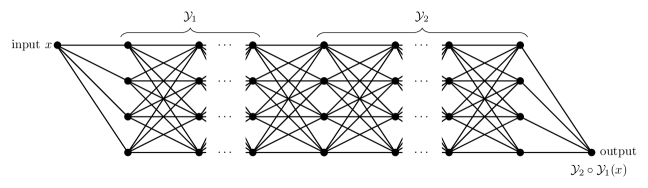
Figure 9: The network computing ${\cal Y}_{2}\circ{\cal Y}_{1}$.

The concatenated network has the same input and first $L_{1}$ hidden layers as the network ${\cal N}_{1}$. Its $(L_{1}+1)$-st layer is the same as the first hidden layer of the network ${\cal N}_{2}$. The weights between the $L_{1}$-st and $(L_{1}+1)$-st layer are the output weights of ${\cal Y}_{1}$, multiplied by the input weights for the first hidden layer of ${\cal Y}_{2}$.

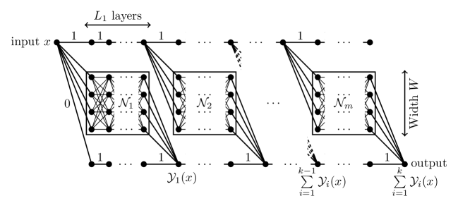
Figure 10: The computational graph of the special $\mathrm{ReLU}$ network producing $\sum_{j=1}^{k}{\cal Y}_{j}$.

The remainder of the concatenated network is the same as the remaining layers of ${\cal N}_{2}$. Clearly, the resulting network will have $n=L_{1}+\cdots+L_{k}$ hidden layers.

To show (14), we concatenate the networks ${\cal N}_{1},\ldots,{\cal N}_{k}$ as shown in Figure 10 by adding a source channel and a collation channel. The resulting network is a special network with width $W+2$ and depth $L_{1}+\cdots+L_{k}$.

Finally, for (15), we concatenate the networks ${\cal N}_{1},\ldots,{\cal N}_{k}$ by adding an extra layer after each ${\cal N}_{j}$ to perform the $\mathrm{ReLU}$ operation on its output, see Figure 11. The rest of the construction is similar to the one for (14).

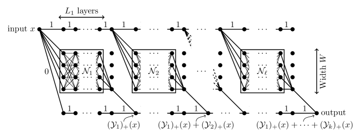
Figure 11: The computational graph of the special $\mathrm{ReLU}$ network producing $\sum_{j=1}^{k}({\cal Y}_{j})_{+}$.

$\Box$

The following two results will also be needed later. We use the notation $g^{\circ k}$ to denote the function which results when $g$ is composed with itself $k$ times.

Proposition 4.3.

If $T\in\Upsilon^{{\rm w},L}$, $2\leq{\rm w}\leq W$, then $S=\sum_{i=1}^{m}a_{i}T^{\circ i}$ can be produced by a special $\mathrm{ReLU}$ network with width $W+2$ and depth $Lm$ , that is $S\in\overline{\underline{\Upsilon}}^{W+2,Lm}$.

Proof: First, note that we have the inclusion $\Upsilon^{{\rm w},L}\subset\Upsilon^{W,L}$ for every $2\leq{\rm w}\leq W$. We can always assign zero weights and biases to any selected nodes of the network producing $\Upsilon^{W,L}$, and therefore we can always assume that $T\in\Upsilon^{W,L}$. We adjust the network generating $T^{\circ m}$ encountered in the proof of (13). We augment it to a special network in such a way that, after the computation of each of the $T^{\circ i}$, we place $a_{i}T^{\circ i}(x)$ into the collation channel, see Figure 12.

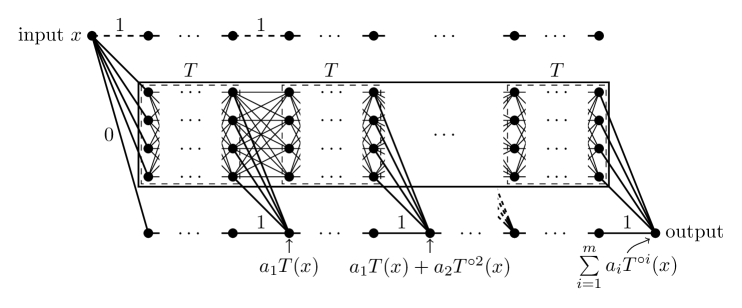
Figure 12: The computational graph of the special $\mathrm{ReLU}$ network producing S.

The source channel is not needed in this case, but we include it nonetheless since it will be used when creating the sum of $S$ with another function. $\Box$

Proposition 4.4.

If $T\in\Upsilon^{W_{1},\ell}$, $g\in\Upsilon^{W_{2},\ell}$, and $W_{1}+W_{2}=W$, then $S_{g}=\sum_{i=1}^{m}a_{i}g(T^{\circ i})$ can be produced by a special $\mathrm{ReLU}$ network with width $W+2$ and depth $\ell(m+1)$, i.e., $S_{g}\in\overline{\underline{\Upsilon}}^{W+2,\ell(m+1)}$.

Proof: As before, we use the network of width $W_{1}$ generating $T^{\circ m}$. For the other $W_{2}$ channels, we use $m$ copies of the network ${\cal G}$ producing $g$ and combine them as shown in Figure 13. After the computation of each of the $T^{\circ i}$, we place $T^{\circ i}(x)$ as an input in the $i$-th copy of ${\cal G}$ and put $a_{i}$ times its output into the collation channel.

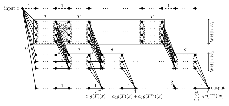
Figure 13: The computational graph of the special $\mathrm{ReLU}$ network producing $S_{g}$.

Again, the source channel is not needed here but can be used at a later time. $\Box$

5 $\mathrm{ReLU}$ networks efficiently produce functions with self similarity

Having established that $\mathrm{ReLU}$ networks contain sums and compositions of CPwL functions, we show that they also contain CPwL functions with certain self-similar patterns. We formalize this structure below.

Let $0<\xi_{1}<\xi_{2}<\cdots<\xi_{k}<1$ be a fixed set of breakpoints and let $S$ be any element of ${\cal S}({\bf\xi}):={\cal S}(0,\xi_{1},\ldots,\xi_{k},1)$. In particular, $S$ vanishes outside of $[0,1]$. We think of $S$ as a pattern. It is easy and cheap for $\mathrm{ReLU}$ networks to replicate this pattern on many intervals. To describe this, let $\{J_{1},\dots,J_{m}\}$ denote a collection of $m$ intervals contained in $[0,1]$ whose interiors are pairwise disjoint. We order these intervals from left to right. We say that a CPwL function $F$ is self similar with pattern $S\in{\cal S}({\bf\xi})$ if

$$F(x)=\sum_{i=1}^{m}S(h_{i}(x-a_{i})),\quad x\in[0,1],$$ (16)

where $J_{i}=[a_{i},b_{i}]$ and $h_{i}=|J_{i}|^{-1}$, $i=1,\dots,m$. Thus, the function $F$ consists of a dilated version of $S$ on each of the $m$ intervals $J_{i}$. It has roughly $km$ breakpoints but is only described by $2(k+m)$ parameters. We show below that, in order to produce such a function $F$, $\mathrm{ReLU}$ networks only need a number of parameters of the order $k+m$, and not $km$ as would be naively inferred by regarding $F$ as an element of $\Sigma_{km}$.

Theorem 5.1.

Let $W\geq 8$. Any self-similar function $F$ of the form (16) with $S\in{\cal S}({\bf\xi})\subset\Sigma_{k}$ belongs to $\overline{\underline{\Upsilon}}^{W,L}$, for a suitable value of $L$ that satisfies $n(W,L)\leq C_{1}(k+m)+C_{2}W^{2}$ for some absolute constants $C_{1},C_{2}>0$.

Proof: We start with the case when $S$ is nonnegative and the intervals $J_{i}=[a_{i},b_{i}]$ (not just their interiors) are disjoint. For each $i=1,\ldots,m$, we introduce a point $c_{i}$ in the interval $(b_{i},a_{i+1})$, where $a_{m+1}:=1$. We consider the hat function ${\cal H}_{i}$ which is zero outside $[a_{i},c_{i}]$, equal to one at $b_{i}$, and linear on $[a_{i},b_{i}]$ and $[b_{i},c_{i}]$, as well as the hat function $\hat{\cal H}_{i}$ which is zero outside $[b_{i},a_{i+1}]$, equal to one at $c_{i}$, and linear on $[b_{i},c_{i}]$ and $[c_{i},a_{i+1}]$. In the case when $b_{m}=1$, we cannot construct ${\cal H}_{m}$ and $\hat{\cal H}_{m}$ as above, and instead set ${\cal H}_{m}(x)=\frac{1}{1-a_{m}}(x-a_{m})_{+}$ and $\hat{\cal H}_{m}(x)=0$. With $\hat{S}(x):=S(1-x)$, we claim that

$$F=\big{(}S\circ T-\hat{S}\circ\hat{T}\big{)}_{+},\qquad\quad\text{where}\quad T:=\sum_{i=1}^{m}{\cal H}_{i},\qquad\hat{T}:=\sum_{i=1}^{m}\hat{\cal H}_{i}.$$

This can be easily verified by separating into the three cases $x\in[a_{i},b_{i}]$, $x\in[b_{i},c_{i}]$, and $x\in[c_{i},a_{i+1}]$. According to Theorem 3.1, we have $S,\hat{S}\in\Upsilon^{W-4,L^{\prime}}$ with either $W^{2}L^{\prime}\asymp n(W-4,L^{\prime})\leq C^{\prime}k$ or $L^{\prime}=2$, and $T,\hat{T}\in\Upsilon^{W-4,L^{\prime\prime}}$ with either $W^{2}L^{\prime\prime}\asymp n(W-4,L^{\prime\prime})\leq C^{\prime\prime}m$ or $L^{\prime\prime}=2$. Then, by Proposition 4.2, we obtain that both $S\circ T,\hat{S}\circ\hat{T}\in\Upsilon^{W-4,L^{\prime}+L^{\prime\prime}}$, that their difference $S\circ T-\hat{S}\circ\hat{T}\in\overline{\underline{\Upsilon}}^{W-2,2(L^{\prime}+L^{\prime\prime})}\subset\Upsilon^{W-2,2(L^{\prime}+L^{\prime\prime})}$. At last, the function $F=\big{(}S\circ T-\hat{S}\circ\hat{T}\big{)}_{+}\in\overline{\underline{\Upsilon}}^{W,L^{\prime\prime\prime}}$, where $L^{\prime\prime\prime}=1+2(L^{\prime}+L^{\prime\prime})$, and therefore $n(W,L^{\prime\prime\prime})\asymp W^{2}L^{\prime\prime\prime}\leq c_{1}(k+m)+c_{2}W^{2}$.

Now, in the case of a general pattern $S$ with $k$ breakpoints, we write $S=S_{+}-S_{-}$, where $S_{+},S_{-}$ are nonnegative, vanish outside $[0,1]$, and have $k^{\prime}\leq 2k$ breakpoints. We also decompose each sum (16) corresponding to $S_{+}$ and $S_{-}$ into a sum over odd indices and a sum over even indices to guarantee disjointness of the underlying intervals. In this way, $F$ is represented as a sum of the $\mathrm{ReLU}$ of four functions of the form $(S_{i}\circ T_{i}-\hat{S}_{i}\circ\hat{T}_{i})$ each of them belonging to $\overline{\underline{\Upsilon}}^{W-2,2(L^{\prime}+L^{\prime\prime})}$ and according to Proposition 4.2, it follows that $F\in\overline{\underline{\Upsilon}}^{W,L}$, where $L=4+8(L^{\prime}+L^{\prime\prime})$. Finally, a parameter count gives

$$n(W,L)\asymp W^{2}L=4W^{2}+8W^{2}(L^{\prime}+L^{\prime\prime})\leq C_{1}(k+m)+C_{2}W^{2},$$

where $C_{1}$ and $C_{2}$ are absolute constants and concludes the proof. $\Box$

Remark 5.1.

The above argument also works if the condition $S\in{\cal S}({\bf\xi})\subset\Sigma_{k}$ is replaced by $S\in\Upsilon^{W-4,L}$, where $S(0)=S(1)$ and $n(W-4,L)\leq Ck$, with $C$ being an absolute constant.

6 $\mathrm{ReLU}$ networks are at least as expressive as Fourier-like sums

In this section, we show that $\mathrm{ReLU}$ networks can efficiently produce linear combinations of functions from a certain Riesz basis that emulates the trigonometric basis. The main point to emphasize here is that the linear combinations we consider can involve any of these basis functions not just the first consecutive ones. Such a linear combination consisting of $n$ basis functions is commonly referred to as an $n$ term approximation from a dictionary (a basis in our case). Approximation by such sums is a classic example of nonlinear approximation.

To describe the Riesz basis we have in mind, we consider the functions ${\cal C},{\cal S}:[0,1]\to\mathbb{R}$, given by

$${\cal C}(x):=\left\{\begin{matrix}1-4x,&x\in[0,1/2),\\ 4x-3,&x\in[1/2,1],\end{matrix}\right.\qquad{\cal S}(x):=\left\{\begin{matrix}4x,&x\in[0,1/4),\\ 2-4x,&x\in[1/4,3/4),\\ 4x-4,&x\in[3/4,1].\end{matrix}\right.$$

Next, for each $k\geq 1$, we introduce ${\cal C}_{k},{\cal S}_{k}:[0,1]\to\mathbb{R}$, defined for any $x\in[0,1]$ by

$${\cal C}_{k}(x):={\cal C}(kx-\lfloor kx\rfloor),\qquad{\cal S}_{k}(x):={\cal S}(kx-\lfloor kx\rfloor).$$

Examples of representatives of this family of functions are depicted in Figure 14.

Figure 14: The graphs of ${\cal C}$, ${\cal S}$, ${\cal C}_{3}$, and ${\cal S}_{3}$.

The system ${\cal F}:=({\cal C}_{k},{\cal S}_{k})_{k\geq 1}$ is an important example of a family of CPwL functions, since it forms a Riesz basis for $L_{2}^{0}[0,1]$, the set of square integrable functions on $[0,1]$ with zero mean. Namely, the following statement holds.

Proposition 6.1.

The system $({\cal C}_{k},{\cal S}_{k})_{k\geq 1}$ is a Riesz basis for $L_{2}^{0}[0,1]$, that is it spans $L_{2}^{0}[0,1]$ and there are absolute constants $c,C>0$ such that, for any two sequences $a,b\in\ell_{2}(\mathbb{N})$ of real numbers we have,

$$c\sum_{k\geq 1}(a_{k}^{2}+b_{k}^{2})\leq\bigg{\|}\sum_{k\geq 1}(a_{k}{\cal C}_{k}+b_{k}{\cal S}_{k})\bigg{\|}_{L_{2}[0,1]}^{2}\leq C\sum_{k\geq 1}(a_{k}^{2}+b_{k}^{2}).$$ (17)

Proof: The proof of this statement is deferred to the appendix. $\Box$

The following theorem shows how we can produce via $\mathrm{ReLU}$ networks $2k$-term linear combinations of elements from ${\cal F}$ with a good control on the depth $L$.

Theorem 6.2.

Let $W\geq 6$. For every $k\geq 1$, and set of indices $\Lambda\subset\mathbb{N}$ with $|\Lambda|=k$, the set

$${\cal F}_{\Lambda}:=\bigg{\{}\sum_{j\in\Lambda}(a_{j}\mathcal{C}_{j}+b_{j}\mathcal{S}_{j}),\;a_{j},b_{j}\in\mathbb{R},j\in\Lambda,\,\ |\Lambda|=k\bigg{\}}\subset\Upsilon^{W,L},$$

where $\Upsilon^{W,L}$ is produced by a $\mathrm{ReLU}$ network of depth

$$L=2\left\lceil\frac{k}{\lfloor\frac{W-2}{4}\rfloor}\right\rceil(\lceil\log_{2}(\lambda)\rceil+2),\qquad\quad\text{with}\quad\lambda:=\max\{j:\,j\in\Lambda\}.$$

Proof: With $H$ denoting the hat function from Figure 2, we observe that $H^{\circ m}=H\circ\cdots\circ H$ is a sawtooth function, see Figure 15, i.e., a CPwL function taking alternatively the values $0$ and $1$ at its breakpoints $\ell 2^{-m}$, $\ell=0,1,\ldots,2^{m}$. Note that the restriction of the function $(2^{m}x-\lfloor 2^{m}x\rfloor)$ on each interval $[\ell 2^{-m},(l+1)2^{-m})$ is a linear function passing through $\ell 2^{-m}$ with slope $1$. Since ${\cal C}(0)={\cal C}(1)$, one can easily see that

$$\mathcal{C}_{2^{m}}(x)={\cal C}(2^{m}x-\lfloor 2^{m}x\rfloor)=\mathcal{C}(H^{\circ m}(x)).$$

Since $H$ and $\mathcal{C}=1-2H$ can both be produced by $\mathrm{ReLU}$ networks of width $2$ and depth $1$, it follows from (13) that $\mathcal{C}_{2^{m}}\in\Upsilon^{2,m+1}$, $m=0,1,\dots$.

Next, given an integer $j$, we find the smallest $m$ with the property $j\leq 2^{m}$. In view of $\mathcal{C}_{j}(x)=\mathcal{C}_{2^{m}}(j2^{-m}x)$, $j\leq 2^{m}$, we also derive that $\mathcal{C}_{j}\in\Upsilon^{2,m+1}=\Upsilon^{2,\lceil\log_{2}j\rceil+1}$. Likewise, because $\mathcal{S}$ can be produced by a $\mathrm{ReLU}$ network of width $2$ and depth $2$ (by virtue of the identity $\mathcal{S}(x)=\mathcal{C}_{2}(x/2+3/8)$, $x\in[0,1]$), we can show that $\mathcal{S}_{j}\in\Upsilon^{2,m+2}=\Upsilon^{2,\lceil\log_{2}j\rceil+2}$. Thus, we have established that, according to (14), for each $j\in\Lambda$,

$$a_{j}\mathcal{C}_{j}+b_{j}\mathcal{S}_{j}\in\overline{\underline{\Upsilon}}^{4,2\lceil\log_{2}j\rceil+4}\subset\Upsilon^{4,2(\lceil\log_{2}\lambda\rceil+2)},\quad\text{where}\quad\lambda:=\max\{j:\,j\in\Lambda\}.$$

Let us denote by $p:=2(\lceil\log_{2}\lambda\rceil+2)$. By stacking networks on top of each other, a sum of $\lfloor\frac{W-2}{4}\rfloor$ terms $a_{j}\mathcal{C}_{j}+b_{j}\mathcal{S}_{j}$ belongs to the set $\Upsilon^{4\lfloor\frac{W-2}{4}\rfloor,p}\subset\Upsilon^{W-2,p}$. Then, again by (14), a sum of $k\leq\lceil k/\lfloor\frac{W-2}{4}\rfloor\rceil\times\lfloor\frac{W-2}{4}\rfloor$ elements $a_{j}\mathcal{C}_{j}+b_{j}\mathcal{S}_{j}$ belongs to $\Upsilon^{W,\lceil k/\lfloor(W-2)/4\rfloor\rceil p}$, as announced. $\Box$

Remark 6.1.

Describing the set ${\cal F}_{\Lambda}$ requires $2k$ parameters, while the number of parameters $n(W,L)$ for the set $\Upsilon^{W,L}$ above has the order of $W^{2}L\asymp Wk\log_{2}(\lambda)$. Ignoring the logarithmic factor, this is comparable with $2k$ only when the width $W$ is viewed as an absolute constant.

We can take another approach and rather than stacking the networks producing ${\cal S}_{j}$ and ${\cal C}_{j}$ on the top of each other, concatenate them into a special network with width $W=4$. This way we will obtain that

$${\cal F}_{\Lambda}\subset\Upsilon^{4,2k(\lceil\log_{2}(\lambda)\rceil+2)}.$$

7 Approximation by (deep) neural networks

So far, we have seen in §3, §5, and §6 that $\mathrm{ReLU}$ networks can produce free knot linear splines, self-similar functions, and expansions in Fourier-like Riesz basis of CPwL functions using essentially the same number of parameters that are used to describe these sets. This implies that $\mathrm{ReLU}$ networks are at least as expressive as any of these sets of functions. In fact, they are at least as expressive as the union of these sets, which intuitively forms a powerful incoherent dictionary.

We are more interested in the approximation power of deep neural networks rather than their expressiveness. Of course, one expects these two concepts are closely related. The remainder of this paper aims at providing convincing results about the approximation power of $\mathrm{ReLU}$ networks that establishes their superiority over the existing and more traditional methods of approximation. We shall do so by concentrating on special $\mathrm{ReLU}$ networks $\overline{\underline{\Upsilon}}^{W+2,L}$ with a fixed width $W+2$. We introduce the notation

$$\overline{\underline{\Upsilon}}_{m}:=\overline{\underline{\Upsilon}}^{W+2,m}\subset\Upsilon^{W+2,m},\qquad\mbox{when}\,\,m\geq 1,$$

and $\overline{\underline{\Upsilon}}_{0}:=\{0\}$, and formally define the approximation family

$$\overline{\underline{\Upsilon}}:=(\overline{\underline{\Upsilon}}_{m})_{m\geq 0}.$$

The number of parameters determining the set $\overline{\underline{\Upsilon}}_{m}$ is $n(W+2,m)\asymp W^{2}m$, and in going further, we shall refer to them as roughly $W^{2}m$. Recall that according to Proposition 3.2, this nonlinear family possesses the following favorable properties:

• Nestedness: $\overline{\underline{\Upsilon}}_{m^{\prime}}\subset\overline{\underline{\Upsilon}}_{m}$ when $m^{\prime}\leq m$;

• Summation property: $\overline{\underline{\Upsilon}}_{m^{\prime}}+\overline{\underline{\Upsilon}}_{m}\subset\overline{\underline{\Upsilon}}_{m^{\prime}+m}$.

7.1 Nonlinear approximation

Let $X$ be any Banach space of functions defined on $[0,1]$. The typical examples of $X$ are the $L_{p}[0,1]$ spaces, $1\leq p\leq\infty$, $C[0,1]$, Sobolev and Besov spaces. Our only stipulation on $X$, at this point, is that it should contain all continuous piecewise linear functions on $[0,1]$. Given $f\in X$, we define its approximation error when using deep neural networks to be

$$\sigma_{m}(f,\overline{\underline{\Upsilon}})_{X}:=\inf_{S\in\overline{\underline{\Upsilon}}_{m}}\|f-S\|_{X},\quad m\geq 0.$$

Since $\overline{\underline{\Upsilon}}_{0}:=\{0\}$, we have $\sigma_{0}(f,\overline{\underline{\Upsilon}})=\|f\|_{X}$. Given a compact subset $K\subset X$, we define the performance on $K$ to be

$$\sigma_{m}(K,\overline{\underline{\Upsilon}})_{X}:=\sup_{f\in K}\sigma_{m}(f,\overline{\underline{\Upsilon}})_{X},\quad m\geq 0.$$

In other words, the approximation error on the class $K$ is the worst error.

In a similar way, we define approximation error for other approximation families, in particular $\sigma_{m}(f,\Sigma)_{X}$ and $\sigma_{m}(K,\Sigma)_{X}$ when $\Sigma:=(\Sigma_{m})_{m\geq 0}$ is the family of continuous piecewise linear functions. We want to understand the decay rate of $(\sigma_{m}(f,\overline{\underline{\Upsilon}})_{X})_{m\geq 0}$ for individual functions $f$ and of $(\sigma_{m}(K,\overline{\underline{\Upsilon}})_{X})_{m\geq 0}$ for compact classes $K\subset X$ and to compare them with the decay rate for other methods of approximation.

Another common way to understand the approximation power of a specific method of approximation such as neural networks is to characterize the following approximation classes. Given $r>0$, the approximation class ${\cal A}^{r}(\overline{\underline{\Upsilon}})_{X}$, $r>0$, is defined as the set of all functions $f\in X$ for which

$$\|f\|_{{\cal A}^{r}(\overline{\underline{\Upsilon}})_{X}}:=\sup_{m\geq 0}(m+1)^{r}\sigma_{m}(f,\overline{\underline{\Upsilon}})_{X},$$

is finite. While approximation rates other than $(m+1)^{-r}$ are also interesting, understanding the classes ${\cal A}^{r}$, $r>0$, matches many applications in numerical analysis, statistics, and signal processing. The approximation spaces ${\cal A}^{r}(\overline{\underline{\Upsilon}})_{X}$ are linear spaces. Indeed, if $f,g\in{\cal A}^{r}(\overline{\underline{\Upsilon}})_{X}$ and $S_{m},T_{m}\in\overline{\underline{\Upsilon}}_{m}$ provide the approximants to $f,g$ satisfying

$$\|f-S_{m}\|_{X}\leq M(m+1)^{-r}\quad{\rm and}\quad\|g-T_{m}\|_{X}\leq M^{\prime}(m+1)^{-r},\quad m\geq 0,$$

then $S_{m}+T_{m}$ provides an approximant to $f+g$ satisfying

$$\|f+g-(S_{m}+T_{m})\|_{X}\leq(M+M^{\prime})(m+1)^{-r}\leq 2^{r}(M+M^{\prime})(2m+1)^{-r},\quad m\geq 0.$$

Since $S_{m}+T_{m}$ is in $\overline{\underline{\Upsilon}}_{2m}$ , we derive that $f+g\in{\cal A}^{r}(\overline{\underline{\Upsilon}})_{X}$. We notice in passing that $\|\cdot\|_{{\cal A}^{r}(\overline{\underline{\Upsilon}})_{X}}$ is a quasi-norm.

Approximation classes are defined for other methods of approximation in the same way as for neural networks. Thus, given a sequence ${\cal X}:=(X_{m})_{m\geq 1}$ of spaces (linear or nonlinear), we define ${\cal A}^{r}({\cal X})_{X}$ as above with $\overline{\underline{\Upsilon}}$ replaced by ${\cal X}$. The approximation spaces for all classical linear methods of approximation have been characterized for all $r>0$ when $X=L_{p}[0,1]$ space, $1\leq p<\infty$, and $X=C[0,1]$. For example, these approximation classes are known for approximation by algebraic polynomials, by trigonometric polynomials, and by piecewise polynomials on an equispaced partition. Interestingly enough, these characterizations do not expose any advantage of one classical linear method over another. All of these approximation methods have essentially the same approximation classes. For example, the approximation classes ${\cal A}^{r}$ for approximation in $C[0,1]$ by piecewise constants on equispaced partition of $[0,1]$ are the ${\rm Lip}\ r$ spaces when $0<r\leq 1$. Here, the space Lip $r$ is specified by the condition

$$|f(x)-f(y)|\leq M|x-y|^{r}$$

and the smallest $M\geq 0$ for which this holds is by definition the semi-norm $|f|_{{\rm Lip}\ r}$. The space ${\cal A}^{r}$, $0<r<1$, remains the same if we use trigonometric polynomials of degree $m$. The notion of Lipschitz spaces can be extended to $r>1$ and then can be used to characterize approximation spaces ${\cal A}^{r}$ when $r>1$. We do not go into more detail on approximation spaces for the classical linear spaces but we refer the reader to [11] for a complete description.

The situation changes dramatically when using nonlinear methods of approximation. There is typically a huge gain in favor of nonlinear approximation in the sense that their approximation classes are much larger than for linear approximation, and so it is easier for a function to have the approximation order $O(m^{-r})$. We give just one example, important for our discussion of neural networks, to pinpoint this difference. It is easy to see that any continuous function of bounded variation is in ${\cal A}^{1}(\Sigma)$. Namely, given such a target function $f$ defined on $[0,1]$ and with total variation one, we partition $[0,1]$ into $m$ intervals such that the variation of $f$ on each of these intervals is $1/m$. Then, the CPwL function which interpolates $f$ at the endpoints of these intervals is in $\Sigma_{m}$ and approximates $f$ with error at most $1/m$. Notice that such functions of bounded variation are far from being in ${\rm Lip}\ 1$ because they can change values quite abruptly. This illustrates the central theme of nonlinear approximation that their approximation spaces are much larger than their linear counterparts. We refer the reader to [8] for an overview of nonlinear approximation.

7.2 Approximation of classical smoothness spaces

Let us start this section by revisiting Theorem 3.1, which states that

$$\Sigma_{m}\subset\Upsilon^{W,\frac{C}{W^{2}}m},\quad m\geq q(W-2),$$

and

$$\Sigma_{m}\subset\overline{\underline{\Upsilon}}^{W,2},\quad 1\leq m<q(W-2),$$

where $q=2$ when $2\leq W<7$ and otherwise $q=\lfloor\frac{W-2}{6}\rfloor$. This follows from the simple observation that $W^{2}L\asymp n(W,L)\leq Cm$, when $m\geq q(W-2)$. In addition, for any $m$ we can embed $\Upsilon^{W,m}\subset\overline{\underline{\Upsilon}}^{W+2,m}=\overline{\underline{\Upsilon}}_{m}$ by adding a source and collation channel. Hence, in the view of the new notation, Theorem 3.1 can be restated the following way.

Theorem 7.1.

For $m\geq q(W-2)$, we have

$$\Sigma_{m}\subset\overline{\underline{\Upsilon}}_{\gamma m},\quad\text{where}\quad\gamma=\gamma(W)=\frac{C}{W^{2}},$$

and thus for any $f\in C[0,1]$

$$\sigma_{\gamma m}(f,\overline{\underline{\Upsilon}})_{C[0,1]}\leq\sigma_{m}(f,\Sigma)_{C[0,1]}.$$

For $1\leq m<q(W-2)$,

$$\Sigma_{m}\subset\overline{\underline{\Upsilon}}_{2},$$

and thus for any $f\in C[0,1]$ we have $\sigma_{2}(f,\overline{\underline{\Upsilon}})_{C[0,1]}\leq\sigma_{m}(f,\Sigma)_{C[0,1]}$.

Therefore, all approximation results that involve the error of best approximation $\sigma_{m}(f,\Sigma)_{C[0,1]}$ by the family $\Sigma$ of free knot linear splines will hold for the error of best approximation $\sigma_{\gamma m}(f,\overline{\underline{\Upsilon}})_{C[0,1]}$ by the family $\overline{\underline{\Upsilon}}$.

While we do not expect improvement in the approximation power of classical smoothness classes when using neural networks, there is a little twist here that was exposed in the work of Yarotsky [32]. He proved that for $W=5$,

$$\sup_{f\in{\rm Lip}\ 1}\inf_{S\in\Upsilon^{W,m}}\|f-S\|_{C[0,1]}\leq C\frac{|f|_{{\rm Lip}\ 1}}{m\ln m}.$$

Since $\Upsilon^{W,m}\subset\overline{\underline{\Upsilon}}_{m}$ (by just adding a source and collation channel), his result can be restated using our notation as the following result for approximating functions in ${\rm Lip}\ 1$ by $\mathrm{ReLU}$ networks

$$\sigma_{m}(f,\overline{\underline{\Upsilon}})_{C[0,1]}\leq C(W)\frac{|f|_{{\rm Lip}\ 1}}{m\ln m},\quad m\geq 2,$$ (18)

in the particular case $W=5$. Note that the number of parameters describing $\overline{\underline{\Upsilon}}_{m}$ is roughly $W^{2}m$ , and the surprise in (18) is the favorable appearance of the logarithm. Indeed, for all other standard methods of linear or nonlinear approximation depending on $Cm$ parameters, including $\Sigma$, there is a function $f\in{\rm Lip}\ 1$ which cannot be approximated with accuracy better than $c/m$, $m\geq 1$.

7.2.1 The space Lip $\alpha$

Yarotsky’s theorem can be generalized in many ways. We begin by discussing the Lip $\alpha$ spaces. For this, we isolate a simple remark about the Kolmogorov entropy of the unit ball of ${\rm Lip}\ \alpha$. Let $K_{\alpha}$ be the set of functions with $|f|_{{\rm Lip}\ \alpha}\leq 1$ vanishing at the endpoints $0$ and $1$.

Lemma 7.2.

For each $0<\alpha\leq 1$ and for each integer $k\geq 2$, there are at most $3^{k}$ patterns $S_{1},\dots,S_{3^{k}}$ from ${\cal S}(\xi)$, $\xi=(0,\frac{1}{k},\dots,\frac{k-1}{k},1)$, such that whenever $g\in K_{\alpha}$, there is a $j\in\{1,\dots,3^{k}\}$ with

$$\|g-S_{j}\|_{C[0,1]}\leq 2h^{\alpha},\quad h:=\frac{1}{k}.$$ (19)

In other words, the set $K_{\alpha}$ can be covered by $3^{k}$ balls in $C[0,1]$ of radius $2k^{-\alpha}$ with centers from ${\cal S}(\xi)$.

Proof: We consider the following set ${\cal P}$ of patterns from ${\cal S}(\xi)$. For $T$ to be in ${\cal P}$, we require that $T(\xi_{j})=m_{j}h^{\alpha}$, with $m_{0},\dots,m_{k}$ integers satisfying the conditions

$$m_{0}=m_{k}=0,\quad|m_{j}-m_{j-1}|\leq 1,\quad j=1,\dots,k.$$ (20)

There are at most $3^{k}$ such patterns, i.e., $\#({\cal P})\leq 3^{k}$.

For the proof of our claim, given $g\in K_{\alpha}$, we first notice that $|g(\xi_{j})-g(\xi_{j-1})|\leq h^{\alpha}$, $j=1,\dots,k$. We then approximate $g$ by the CPwL function $S\in{\cal S}(\xi)$, where the values $S(\xi_{j})$ are of the form $\beta_{j}h^{\alpha}$, $\beta_{j}\in\mathbb{Z}$, and are chosen so that $S(\xi_{j})=\beta_{j}h^{\alpha}$ is the closest to $g(\xi_{j})$, $j=1,\ldots,k$. Note that this gives $\beta_{0}=\beta_{k}=0$ since $g(\xi_{0})=0=g(\xi_{k})$ and

$$\left|S(\xi_{j})-g(\xi_{j})\right|\leq h^{\alpha}/2.$$ (21)

When assigning the values $S(\xi_{j})$, starting with $S(\xi_{0})=0$ and moving from left to right, if it happens that there are two possible choices for $\beta_{j}$ (which happens if $g(\xi_{j})\pm h^{\alpha}/2$ is an integer multiple of $h^{\alpha}$), we select the $\beta_{j}$ that is closest to the already determined $\beta_{j-1}$. Since

$$\left|\beta_{j}-\beta_{j-1}\right|h^{\alpha} = \left|S(\xi_{j})-S(\xi_{j-1})\right|$$

$$\leq \left|S(\xi_{j})-g(\xi_{j})\right|+\left|g(\xi_{j})-g(\xi_{j-1})\right|+\left|g(\xi_{j-1})-S(\xi_{j-1})\right|$$

$$\leq h^{\alpha}/2+h^{\alpha}+h^{\alpha}/2=2h^{\alpha},$$

we have $|\beta_{j}-\beta_{j-1}|\leq 2$. But the case of equality is not possible since it would mean that at step $j$ we have not selected $\beta_{j}$ to be the closest to $\beta_{j-1}$. Therefore $|\beta_{j}-\beta_{j-1}|\leq 1$, and thus (20) holds, i.e., the constructed approximant $S$ is a pattern from ${\cal P}$. Finally, we notice that any pattern from ${\cal P}$ has slopes with absolute value at most $h^{\alpha-1}$. Hence, for any $x\in[0,1]$, picking the point $\xi_{j}$ the closest to $x$, we have

$$|g(x)-S(x)|\leq|g(x)-g(\xi_{j})|+|g(\xi_{j})-S(\xi_{j})|+|S(\xi_{j})-S(x)|\leq(h/2)^{\alpha}+h^{\alpha}/2+h^{\alpha-1}(h/2)\leq 2h^{\alpha},$$

where we used (21) and the fact that $|x-\xi_{j}|\leq h/2$. Taking the maximum over $x\in[0,1]$ establishes (19) and concludes the proof. $\Box$

The following theorem generalizes (18) to Lip $\alpha$ spaces.

Theorem 7.3.

Let $W\geq 8$. If $X=C[0,1]$ and $f\in{\rm Lip}\ \alpha$, $0<\alpha\leq 1$, then

$$\sigma_{m}(f,\overline{\underline{\Upsilon}})_{X}\leq C(W)\frac{|f|_{{\rm Lip}\ \alpha}}{(m\ln m)^{\alpha}},\quad m\geq 2.$$ (22)

Proof: Without loss of generality, we can assume that $|f|_{{\rm Lip}\ \alpha}=1$. Fixing $f$ and $m$, we first choose $T$ as the piecewise linear function which interpolates $f$ at the equally spaced points $x_{0},\dots,x_{m}$, where $x_{i}:=i/m$, $i=0,\dots,m$. Since $f$ and $T$ agree at the endpoints of the interval $J_{i}:=[x_{i},x_{i+1}]$, the slope of $T$ on $J_{i}$ has absolute value at most $m^{1-\alpha}$. Therefore,

$$|T(x)-T(y)|\leq m^{1-\alpha}|x-y|\leq|x-y|^{\alpha},\quad x,y\in J_{i},$$

and hence $T$ is also in Lip $\alpha$ with semi-norm at most one on each of these intervals.

We now define $g:=f-T$ and write $g=\sum_{i=1}^{m}g\chi_{J_{i}}$. Each $g_{i}:=g\chi_{J_{i}}$ is a function in Lip $\alpha$ with $|g_{i}|_{{\rm Lip}\ \alpha}\leq 2$. Let $k$ be the largest integer such that $3^{k}k\leq m$ and let ${\cal P}=\{S_{1},\dots,S_{3^{k}}\}$ be the set of the $3^{k}$ patterns given by Lemma 7.2. Applying this lemma to each of the functions $\bar{g}_{i}:[0,1]\rightarrow\mathbb{R}$, defined by $\bar{g}_{i}(x):=2^{-1}m^{\alpha}g_{i}((x+i)/m)\in K_{\alpha}$, we find a pattern $S_{j_{i}}\in{\cal P}$, $S_{j_{i}}:[0,1]\rightarrow\mathbb{R}$, such that

$$\|\bar{g}_{i}-S_{j_{i}}\|_{C[0,1]}\leq 2k^{-\alpha}.$$

Shifting back to the interval $J_{i}$ provides a function $S_{j_{i}}\in{\cal P}$ such that

$$|g_{i}(x)-2m^{-\alpha}S_{j_{i}}(m(x-x_{i}))|\leq 4{(km)^{-\alpha}},\quad x\in J_{i},$$

and therefore the function $\hat{T}$ given by

$$\hat{T}(x):=T(x)+2m^{-\alpha}\sum_{i=1}^{m}S_{j_{i}}(m(x-x_{i}))$$ (23)

approximates $f$ to accuracy $4(km)^{-\alpha}$ in the uniform norm.

Since there are $3^{k}<m$ patterns, some of them must be repeated in the sum (23). For each $j=1,\ldots,3^{k}$, we consider the (possibly empty) set of indices $\Lambda_{j}=\{i\in\{1,\ldots,m\}:j_{i}=j\}$. We have

$$\hat{T}=T+\sum_{j=1}^{3^{k}}T_{j},\qquad\mbox{where}\quad T_{j}:=2m^{-\alpha}\sum_{i\in\Lambda_{j}}S_{j}(m(x-x_{i})).$$

Since $T\in\Sigma_{m}$, Theorem 3.1 says that $T$ belongs to $\overline{\underline{\Upsilon}}^{W,L_{0}}$ with either $W^{2}L_{0}\asymp n(W,L_{0})\leq C^{\prime}m$ or $L_{0}=2$. According to Lemma 5.1, each function $T_{j}$ is in $\overline{\underline{\Upsilon}}^{W,L_{j}}$ with either $W^{2}L_{j}\asymp n(W,L_{j})\leq C_{1}(k+m_{j})+C_{2}W^{2}$ or $L_{j}=2$, where $m_{j}:=|\Lambda_{j}|$. Therefore, in view of (14), we derive that $\hat{T}$ belongs to $\overline{\underline{\Upsilon}}^{W,L}$ with $L=L_{0}+\sum_{j=1}^{3^{k}}L_{j}$, and

$$L=L_{0}+\sum_{j=1}^{3^{k}}L_{j}\leq\frac{1}{W^{2}}\left(C^{\prime}m+C_{1}3^{k}k+C_{1}\sum_{j=1}^{3^{k}}m_{j}\right)+C_{3}3^{k}\leq\left(\frac{\tilde{C}_{1}}{W^{2}}+\tilde{C}_{2}\right)m=c(W)m,$$

where we have used the facts that $3^{k}k\leq m$ and $\sum_{j=1}^{3^{k}}m_{j}=m$. This shows that $\hat{T}\in\overline{\underline{\Upsilon}}_{c(W)m}$ and in turn that

$$\sigma_{c(W)m}(f,\overline{\underline{\Upsilon}})_{C[0,1]}\leq\|f-\hat{T}\|_{C[0,1]}\leq\frac{4}{(km)^{\alpha}}\leq\frac{\widetilde{C}}{(m\ln m)^{\alpha}},$$

where in the last inequality we have used that $k\geq c\ln m$ since $3^{k+1}(k+1)>m$. Up to the change of $m$ in $c(W)m$, this is the result announced in (22). $\Box$

7.2.2 Other classical smoothness spaces

We can also exhibit a certain logarithmic improvement in the approximation rate for functions in other smoothness classes. Since we do not wish to delve too deeply into the theory of smoothness spaces in the present paper, we illustrate this with just one example.

Theorem 7.4.

Let $W\geq 8$. If $X=C[0,1]$ and $f\in C[0,1]$ satisfies $f^{\prime}\in L_{p}[0,1]$, $1\leq p\leq\infty$, then

$$\sigma_{m}(f,\overline{\underline{\Upsilon}})_{X}\leq C(W)\frac{\|f^{\prime}\|_{L_{p}}}{m(\ln m)^{1-1/p}},\quad m\geq 2,$$ (24)

where $C(W)$ depends also on $p$ (when $p$ is close to one).

Proof: When $p=\infty$, (24) follows from Theorem 7.3 since $f^{\prime}\in L_{\infty}$ is equivalent to $f\in{\rm Lip}\ 1$ and $|f|_{{\rm Lip}\ 1}=\|f^{\prime}\|_{L_{\infty}}$. The case $p=1$ follows from

$$\sigma_{\gamma m}(f,\overline{\underline{\Upsilon}})_{X}\leq\sigma_{m}(f,\Sigma)_{X}\leq\|f^{\prime}\|_{L_{1}}m^{-1},\quad m\geq 1.$$ (25)

Here, the first inequality follows from Theorem 7.1 and the second inequality is a consequence of an estimate (already mentioned) for CPwL approximation of continuous functions of bounded variation, which applies to $f$ since $f^{\prime}\in L_{1}$. Now, given $1<p<\infty$ and $f\in C[0,1]$ with $f^{\prime}\in L_{p}$, for any $t>0$, we can write

$$f=f_{0}+f_{1},$$

where

$$\max\{\|f_{1}^{\prime}\|_{L_{1}},t\|f_{0}^{\prime}\|_{L_{\infty}}\}\leq\|f_{1}^{\prime}\|_{L_{1}}+t\|f_{0}^{\prime}\|_{L_{\infty}}\leq C\|f^{\prime}\|_{L_{p}}t^{1-1/p},$$

and $C$ is a constant depending on $p$ when $p$ is close to $1$. This is a well-known result in interpolation of operators (see [7]). We take $t:=(\ln m)^{-1}$ and find

$$\sigma_{2\gamma m}(f,\overline{\underline{\Upsilon}})_{X} \leq \sigma_{\gamma m}(f_{0},\overline{\underline{\Upsilon}})_{X}+\sigma_{\gamma m}(f_{1},\overline{\underline{\Upsilon}})_{X}$$

$$\leq C(W)\{\|f_{0}^{\prime}\|_{L_{\infty}}(m\ln m)^{-1}+\|f_{1}^{\prime}\|_{L_{1}}m^{-1}\}$$

$$\leq C(W)\|f^{\prime}\|_{L_{p}}\{(m\ln m)^{-1}t^{-1/p}+m^{-1}t^{1-1/p}\}$$

$$\leq C(W)\|f^{\prime}\|_{L_{p}}m^{-1}(\ln m)^{-1+1/p},$$

where we used the summation property for the elements of the family $\overline{\underline{\Upsilon}}$. The second inequality followed from Theorem 7.3 with $\alpha=1$ and from the estimate (25). $\Box$

7.3 The power of depth

The previous subsection showed that functions taken from classical smoothness spaces typically enjoy some mild improvement in approximation efficiency when using $\mathrm{ReLU}$ networks rather than more classical methods of approximation. However, this modest gain does not give any convincing reason for the success of deep networks, at least from the viewpoint of their approximation properties. In this subsection, we highlight several classes of functions whose approximation rates by neural networks far exceed their approximation rates by free knots linear splines or any other standard approximation family. Our constructions are based on variants of the following simple observation.

Proposition 7.5.

For functions $f_{k}\in\overline{\underline{\Upsilon}}_{k}$ satisfying $\|f_{k}\|_{C[0,1]}=1$ for all $k\geq 1$ and for a sequence $(\beta_{k})_{k\geq 1}$ in $\ell_{1}(\mathbb{N})$, the function

$$F:=\sum_{k\geq 1}\beta_{k}f_{k}$$

has approximation error satisfying

$$\sigma_{m^{2}}(F,\overline{\underline{\Upsilon}})_{C[0,1]}\leq\sum_{k>m}|\beta_{k}|,\quad m\geq 1.$$

Proof. The function $S_{m}:=\sum_{k=1}^{m}\beta_{k}f_{k}$ belongs to $\overline{\underline{\Upsilon}}_{m^{2}}$, thanks to the summation and inclusion properties for $\overline{\underline{\Upsilon}}$. A triangle inequality gives

$$\|F-S_{m}\|_{C[0,1]}\leq\sum_{k>m}|\beta_{k}|,$$

and the statement follows immediately. $\Box$.

Remark 7.1.

When the functions $f_{k}$ are related to one another, the proposition can be improved by replacing $m^{2}$ with a smaller quantity. For example, if $f_{k}=\phi^{\circ k}$ for a fixed function $\phi$ in $\Upsilon^{{\rm w},\ell}$, with width $2\leq{\rm w}\leq W-2$, and fixed depth $\ell$, then Proposition 4.3 reveals that $m^{2}$ can be changed to $\ell m$.

We now present some classes of such functions $F$ that are well approximated by $\mathrm{ReLU}$ networks. For the most part, these functions cannot be well approximated by standard approximation families.

7.3.1 The Takagi class of functions

For our first set of examples, let us recall that functions of the form

$$F=\sum_{k\geq 1}t^{k}g(\psi^{\circ k}),\quad|t|<1,$$ (26)

with $\psi:[0,1]\to[0,1]$ and $g:[0,1]\to\mathbb{R}$, provide primary examples of self similar functions and dynamical systems [33]. If $g\in\Upsilon^{W_{1},\ell}$ and $\psi\in\Upsilon^{W_{2},\ell}$, with $W_{1}+W_{2}=W$, Proposition 4.4 implies that the partial sum $S_{m}:=\sum_{k=1}^{m}t^{k}g(\psi^{\circ k})$ belongs to $\overline{\underline{\Upsilon}}^{W,\ell(m+1)}\subset\overline{\underline{\Upsilon}}_{\ell(m+1)}$. Therefore, in this case, the function $F$ defined via (26) is approximated by the partial sum $S_{m}$ with exponential accuracy by $\mathrm{ReLU}$ networks, that is

$$\sigma_{\ell(m+1)}(F,\overline{\underline{\Upsilon}})_{C[0,1]}\leq Ct^{m+1},\quad|t|<1.$$

Figure 15: The graphs of $H$, $H^{\circ 2}$, and $H^{\circ 3}$.

Now, we consider a special class of functions. For this purpose, we recall that the hat function $H\in\Upsilon^{2,1}$ and its $k$-fold composition $H^{\circ k}:=H\circ H\circ\cdots\circ H$, according to the composition property (13), belongs to $\overline{\underline{\Upsilon}}^{2,k}$. On the other hand, the same function $H^{\circ k}$ is in $\Sigma_{n}$ only if $n$ is exponential in $k$. For an absolutely summable sequence $(c_{k})_{k\geq 1}$ of real numbers, we consider continuous functions $F$ of the form

$$F:=\sum_{k\geq 1}c_{k}H^{\circ k},$$

approximations to which are produced by the special $\mathrm{ReLU}$ networks shown in Figure 16. The collection of all such functions is called the Takagi class. It contains a number of interesting and important examples. A good source of information on the Takagi class is [1], from which the two examples below are taken.

Figure 16: The computation graph associated to the approximation of the Takagi class.

For the first example, we take $c_{k}:=2^{-k}$, which gives the Takagi function

$$T:=\sum_{k\geq 1}2^{-k}H^{\circ k}.$$

From Remark 7.1, we have

$$\sigma_{m}(T,\overline{\underline{\Upsilon}})_{X}\leq 2^{-m},\quad m\geq 1,$$

and so theoretically $T$ can be approximated with exponential accuracy by $\mathrm{ReLU}$ networks with roughly $W^{2}m$ parameters. In practice, see Figure 16, we can approximate it using $m$ parameters. However, $T$ is nowhere differentiable and so it has very little smoothness in the classical sense. This means that all of the traditional methods of approximation will fail miserably to approximate it. Note that the function $T$ has self similarity, in that it satisfies a simple refinement equation.

Other examples take a highly lacunary sequence of coefficients and thereby construct functions in the Takagi class that do not satisfy a Lipschitz condition of any order and yet they can be approximated to exponential accuracy by $\overline{\underline{\Upsilon}}$. Many functions from the Takagi class are fractals, in the sense that the Hausdorff dimension of their graph is strictly greater than one.

We do not go into the Takagi class more deeply but refer the reader to [1, 13] where the properties and applications of the Takagi functions are given as well as numerous examples of similar constructions. The main point to draw from these examples is that the approximation classes ${\cal A}^{r}$ for $r$ large contain many functions which are not smooth in any classical sense.

7.3.2 Analytic functions

Another example in the Takagi class is the function

$$x(1-x)=\sum_{k\geq 1}4^{-k}H^{\circ k}.$$ (27)

This formula is used as a starting point to show that analytic functions are well approximated by deep neural networks (see [31, 20, 12]), as we briefly discuss below.

It follows from (27) that the function $x^{2}$ is approximated with exponential accuracy by $\mathrm{ReLU}$ networks. From this, one derives that all power functions $x^{k}$ also are approximated with exponential accuracy. Then, using the summation property, one concludes that analytic functions and functions in Sobolev spaces are approximated with the same accuracy as their approximation by algebraic polynomials. Similarly, we can approximate functions on $[0,1]$ from their power series representation. The point we emphasize here is the flexibility of $\mathrm{ReLU}$ networks, in that they approximate well functions with little classical smoothness but retain the property of approximating classically smooth functions with the same accuracy as other methods of approximation.

8 Neural network approximation as manifold approximation

Up to this point, we reflected the expressive power and the corresponding approximation power of deep ReLU networks. In other words, we wondered how well the best approximation from $\overline{\underline{\Upsilon}}_{m}$ to a target function performs. An important practical issue is the construction of reasonable methods of approximation that yield near-best approximations to any given target function $f\in X$ with e.g. $X=C[0,1]$.

To discuss this problem, we need to formulate what would be considered a reasonable approximation procedure. The set $\overline{\underline{\Upsilon}}_{m}$ is described by roughly $W^{2}m$ parameters, which are identified by a point in $\mathbb{R}^{m}$. We let $M=M_{m}$ be the mapping that sends $z\in\mathbb{R}^{m}$ to the function $M(z)$ generated by the neural network with the chosen parameters $z$. We view the collection ${\cal M}={\cal M}_{m}$ of all $M(z)$, $z\in\mathbb{R}^{m}$, as an $m$-dimensional manifold. In this context, we also view any approximation method as providing a mapping $a=a_{m}:X\to\mathbb{R}^{m}$ which, for a given $f\in X$, selects the parameters of the network used to approximate $f$. The approximation to $f$ is then

$$A_{m}(f)=M_{m}(a_{m}(f)),\quad n\geq 0.$$

A fundamental question for both theory and numerical practice is what conditions to impose on $a_{m}$ and $M_{m}$ so that the resulting scheme $A_{m}$ is reasonable. In keeping with the notion of numerical stability, we could require that each of these mappings is a Lip $1$ with a fixed constant $\Gamma$ independent of $m$. This means that there is a norm $\|\cdot\|$ on $\mathbb{R}^{m}$ (typically an $\ell_{p}$ norm) such that, for any $f_{1},f_{2}\in X$,

$$\|a_{m}(f_{1})-a_{m}(f_{2})\|\leq\Gamma\|f_{1}-f_{2}\|_{X}.$$

The stability of $M_{m}$ means that, for any $z_{1},z_{2}\in\mathbb{R}^{m}$,

$$\|M_{m}(z_{1})-M_{m}(z_{2})\|_{X}\leq\Gamma\|z_{1}-z_{2}\|.$$

One can lessen the demand on numerical stability to requiring only that the mappings $a_{m}$ and $M_{m}$ are continuous, not necessarily Lipschitz. This weaker assumption was used in the definition of manifold widths [9]. This manifold width of a compact set $K\subset X$ is defined as

$$\delta_{m}(K):=\inf_{(a,M)}\sup_{f\in K}\|f-M(a(f))\|_{X},$$

where the infimum is taken over all continuous maps. It is shown in [10] that this milder requirement still puts a restriction on how well sets characterized by classical smoothness can be approximated. For example, if $K$ is the unit ball of Lip $\alpha$, then $\delta_{m}(K)\geq Cm^{-\alpha}$. Therefore, the logarithmic improvement featured in §7.2 cannot be obtained with continuous selection of parameters. This lack of continuity for some approximation schemes was also recognized in [18]. This may be a crucial point in the framing of recent results on the instability of certain methods for constructing deep network approximations to target functions from data via optimization methods (such as least squares or constrained least squares methods).

9 Appendix

9.1 The matrices of Lemma 3.3

In order to explicitly write the affine transforms $A^{(1)}$ and $A^{(2)}$ that determine the $\mathrm{ReLU}$ net, we describe here one of the possible ways to partition the set of indices $\Lambda$ so that the constant sign and separation properties are satisfied. To do this, we first consider $\Lambda_{+}$ and only the main breakpoints $\xi_{j}$ with indices $j$ for which $j\!\!\mod 3=\ell$. We collect into the set $\Lambda_{i}^{\ell,+}$ all indices $k\in\Lambda_{+}$ that correspond to the $i$-th hat function $H_{i,j}$ associated to a principal breakpoint $\xi_{j}$ with the above mentioned property. Recall that there are $q$ hat functions $H_{i,j}$ associated to each principal breakpoint $\xi_{j}$. We do this for every $\ell=0,1,2$, and $\Lambda_{-}$, and we get the partition

$$\Lambda_{i}^{\ell,+}:=\{s:\,s\in\Lambda_{+}\,\,\text{and}\,\,\phi_{s}=H_{i,j}\,\,\text{with}\,\,j\!\!\!\mod 3=\ell\},$$

$$\Lambda_{i}^{\ell,-}:=\{s:\,k\in\Lambda_{-}\,\,\text{and}\,\,\phi_{s}=H_{i,j}\,\,\text{with}\,\,j\!\!\!\mod 3=\ell\},$$

where $\ell=0,1,2$, $i=1,\ldots,q$. The matrices that determine the special $\mathrm{ReLU}$ network are

$$M^{(1)}=\begin{bmatrix}1&1&\ldots&1&0\end{bmatrix}^{T},\quad b^{(1)}=\begin{bmatrix}0&\xi_{1}&\ldots&\xi_{W-2}&0\end{bmatrix}^{T},$$

$$M^{(2)}=\begin{bmatrix}1&0&\ldots&0&0\\ m_{2,1}^{(2)}&m_{2,2}^{(2)}&\ldots&m_{2,W-1}^{(2)}&0\\ \ldots&\ldots&\\ m_{W-1,1}^{(2)}&m_{W-1,2}^{(2)}&\ldots&m_{W-1,W-1}^{(2)}&0\\ 0&0&\ldots&0&1\end{bmatrix},\quad b^{(2)}=\begin{bmatrix}0\\ b_{2}^{(2)}\\ \ldots\\ b_{W-2}^{(2)}\\ 0\end{bmatrix}$$

$$M^{(3)}=\begin{bmatrix}0&\varepsilon^{(3)}_{1}&\ldots&\varepsilon^{(3)}_{W-2}&1\end{bmatrix},\quad b^{(3)}=0,$$

where $\varepsilon^{(3)}_{k}=1$ if $\Lambda_{k}\subset\Lambda_{+}$, $\varepsilon^{(k)}_{k}=-1$ if $\Lambda_{k}\subset\Lambda_{-}$, and $\varepsilon^{(3)}_{k}=0$ if $\Lambda_{k}=\emptyset$. Next, we demonstrate how to find the entrances of one row in $M^{(2)}$. The rest of the rows are computed likewise. The index $k=1,\ldots,W-2$ in (10) corresponds to a different labeling of the index set

$$\{(i,\ell,+),(i,\ell,-),\,i=1,\ldots,q,\,\ell=0,1,2\},$$

of the particular partition we work with here. We take the index $(1,1,+)$ and compute the corresponding $\tilde{T}$,

$$\tilde{T}:=T_{(1,1+)}=\sum_{s\in\Lambda_{1}^{1,+}}c_{s}\phi_{s}=[\tilde{S}]_{+},$$

see Figure 6, where $\tilde{S}$ is a CPwL function with breakpoints the principal breakpoints $\xi_{1},\ldots,\xi_{W-2}$, with the property

$$\tilde{S}(\xi_{4s+1})=c_{4s+1},\quad\tilde{S}(x_{(4s+1)q-1})=\tilde{S}(x_{(4s+1)q+1})=0,\quad s=0,\ldots,\left\lfloor\frac{W-2}{4}\right\rfloor.$$

Then the entries in the second row in $M^{(2)}$ and $b^{(2)}$ are the coefficients from the representation,

$$\tilde{S}(x)=m_{2,1}^{(2)}x+\sum_{j=2}^{W-2}m_{2,j}^{(2)}(x-\xi_{j})_{+}+b_{2}^{(2)}.$$

9.2 Theorem 3.1, Case $4\leq W\leq 7$

In this case we have to show that for every $n\geq 1$ the set $\Sigma_{n}$ of free knot linear splines with $n$ breakpoints is contained in the set $\Upsilon^{W,L}$ of functions produced by width-$W$ and depth-$L$ $\mathrm{ReLU}$ networks where

$$L=\begin{cases}2\left\lceil\frac{n}{2(W-2)}\right\rceil,\quad&n\geq 2(W-2),\\ 2,&n<2(W-2),\end{cases}$$

and whose number of parameters

$$n(W,L)\leq\begin{cases}Cn,\quad&n\geq 2(W-2),\\ W^{2}+4W+1,&n<2(W-2),\end{cases}$$

where $C$ is an absolute constant. We start with the case $W-2=2$. Given $n\geq 4$, we choose $L:=\lceil\frac{n}{4}\rceil$. If $n<4L$, we add artificial breakpoints so that we represent $T\in\Sigma_{n}\subset\Sigma_{4L}$ as

$$T(x)=ax+b+\sum_{j=1}^{4L}c_{j}(x-\xi_{j})_{+}=ax+b+\sum_{j=1}^{2L}S_{j},\quad S_{j}:=c_{2j-1}(x-\xi_{2j-1})_{+}+c_{2j}(x-\xi_{2j})_{+}.$$

Now we can construct the special $\mathrm{ReLU}$ network $\overline{\underline{\Upsilon}}^{4,2L}$ that generates T via the successive transformations $A^{(j)}$ given by the matrices

$$M^{(1)}=\begin{bmatrix}1&1&1&0\end{bmatrix}^{T},\quad b^{(1)}=\begin{bmatrix}0&-\xi_{1}&-\xi_{2}&0\end{bmatrix}^{T},$$

The $j$th layer, $j=2,\ldots,2L$, produces $S_{j-1}$ in its CC node via the matrix

$$M^{(j)}=\begin{bmatrix}1&0&0&0\\ 1&0&0&0\\ 1&0&0&0\\ 0&c_{2j-3}&c_{2j-2}&1\end{bmatrix},\quad b^{(j)}=\begin{bmatrix}0\\ -\xi_{2j-1}\\ -\xi_{2j}\\ 0\end{bmatrix}.$$

Finally, the output layer is given by the matrix

$$M^{(2L)}=\begin{bmatrix}a&c_{2L-1}&c_{2L}&1\end{bmatrix},\quad b^{(2L)}=b,$$

where the first entry $a$ and the bias $b$ account for the linear function $ax+b$ in $T$. In this case we have $\Sigma_{4L}\subset\overline{\underline{\Upsilon}}^{4,2L}\subset\Upsilon^{4,2L}$, with number of parameters

$$n(4,2L)=40L-7=40\left\lceil\frac{n}{4}\right\rceil-7<10n+33<19n,\quad n\geq 4.$$

For the case $n<4$, we again add artificial breakpoints so that we represent $T\in\Sigma_{n}\subset\Sigma_{4}$ as

$$T(x)=ax+b+\sum_{j=1}^{4}c_{j}(x-\xi_{j})_{+}=ax+b+\sum_{j=1}^{2}S_{j},\quad S_{j}:=c_{2j-1}(x-\xi_{2j-1})_{+}+c_{2j}(x-\xi_{2j})_{+},$$

and as above generate a special $\mathrm{ReLU}$ network $\overline{\underline{\Upsilon}}^{4,2}$ for which $\Sigma_{n}\subset\overline{\underline{\Upsilon}}^{4,2}$, and whose parameters

$$n(4,2)=33=W^{2}+4W+1,\quad W=4.$$

Now, for the case $(W-2)\in\{3,4,5\}$, let us first consider $n\geq 2(W-2)$ and take $L:=\left\lceil\frac{n}{2(W-2)}\right\rceil$. If $n<2(W-2)L$, we add artificial breakpoints so that we represent $T\in\Sigma_{n}\subset\Sigma_{2(W-2)L}$. We do the same construction as in the case $W-2=2$, by dividing the indices $\{1,\ldots,2(W-2)L\}$ into $2L$ groups of $W-2$ numbers, as shown in

$$T(x)=ax+b+\sum_{j=1}^{2(W-2)L}c_{j}(x-\xi_{j})_{+}=ax+b+\sum_{j=1}^{2L}S_{j},\quad S_{j}:=\sum_{i=0}^{W-3}c_{(W-2)j-i}(x-\xi_{(W-2)j-i})_{+},$$

and execute the same construction as before by concatenating the networks producing $S_{j}$. In this case, we have $\Sigma_{n}\subset\Sigma_{2(W-2)L}\subset\overline{\underline{\Upsilon}}^{W,2L}$, and when $n\geq 2(W-2)$,

$$n(W,2L)=2W(W+1)\left\lceil\frac{n}{2(W-2)}\right\rceil-(W-1)^{2}+2<\frac{W(W+1)}{W-2}n+W^{2}+4W+1<25n.$$

When $n<2(W-2)$, we again add artificial breakpoints so that we represent $T\in\Sigma_{n}\subset\Sigma_{2(W-2)}$ as

$$T(x)=ax+b+\sum_{j=1}^{2(W-2)}c_{j}(x-\xi_{j})_{+}=ax+b+\sum_{j=1}^{2}S_{j},\quad S_{j}:=\sum_{i=0}^{W-3}c_{(W-2)j-i}(x-\xi_{(W-2)j-i})_{+},$$

and as above generate a special $\mathrm{ReLU}$ network $\overline{\underline{\Upsilon}}^{W,2}$ with depth $L=2$ for which $\Sigma_{n}\subset\overline{\underline{\Upsilon}}^{W,2}$, and whose parameters

$$n(W,2)=2W(W+1)-(W-1)^{2}+2=W^{2}+4W+1,\quad n<2(W-2).$$

This completes the proof. $\square$

9.3 Proof of Theorem 4.1

Proof: Note that for every $k$-tuple $(\tilde{S}_{k},\cdots,\tilde{S}_{1})\in\Sigma_{n_{k}}\times\cdots\times\Sigma_{n_{1}}$, we can find another $k$-tuple $(S_{k},\ldots,S_{1})\in\Sigma_{n_{k}}\times\cdots\times\Sigma_{n_{1}}$, which we call a representative of the composition, with the properties:

• $S_{j}([0,1])\subset[0,1]$, $j=1,\ldots,k-1$.

• $\tilde{S}_{k}\circ\cdots\circ\tilde{S}_{1}=S_{k}\circ\cdots\circ S_{1}$.

Indeed, if we denote by $m_{1}:=\min_{x\in[0,1]}\tilde{S}_{1}(x)$, $M_{1}:=\max_{x\in[0,1]}\tilde{S}_{1}(x)$, define inductively

$$m_{j}:=\min_{x\in[m_{j-1},M_{j-1}]}\tilde{S}_{j},\quad M_{j}:=\max_{x\in[m_{j-1},M_{j-1}]}\tilde{S}_{j},\quad j=2,\ldots,k-1,$$

and consider the functions

$$S_{1} := \frac{\tilde{S}_{1}-m_{1}}{M_{1}-m_{1}}\in\Sigma_{n_{1}},$$

$$S_{j} := \frac{\tilde{S}_{j}(x(M_{j-1}-m_{j-1})+m_{j-1})-m_{j-1}}{M_{j}-m_{j}}\in\Sigma_{n_{j}},\quad j=2,\ldots,k-1,$$

$$S_{k} := \tilde{S}_{k}(x(M_{k-1}-m_{j-1})+m_{k-1}).$$

The $k$-tuple $(S_{k},\ldots,S_{1})$ will be a representative of the composition $\tilde{S}_{k}\circ\ldots\circ\tilde{S}_{1}$. So, in going further, we will always assume that we are dealing with representatives of all compositions we consider and with $\mathrm{ReLU}$ networks that output these representatives.

Relation (11) follows from Proposition 4.2 and Theorem 3.1. Indeed, if we fix an element in $\Sigma^{n_{k}\circ\cdots\circ n_{1}}:=\{\tilde{S}_{k}\circ\cdots\circ\tilde{S}_{1}:\,\tilde{S}_{j}\in\Sigma_{n_{j}},j=1,\ldots,k\}$ and consider its representative $(S_{k},\ldots,S_{1})$, each $S_{j}$ in the composition $S_{k}\circ\cdots\circ S_{1}$ can be produced by a $\mathrm{ReLU}$ network ${\cal C}_{j}$ with width $W$ and depth

$$L_{j}=2\left\lceil\frac{n_{j}}{\lfloor\frac{W-2}{6}\rfloor(W-2)}\right\rceil,$$

and therefore, part (i) of Proposition 4.2 ensures that $S_{k}\circ\cdots\circ S_{1}\in\Upsilon^{W,\sum_{j=1}^{k}L_{j}}$. A similar estimate as in the proof of Theorem 3.1 yields

$$n(W,L) < 34\sum_{j=1}^{k}n_{j}+2k(W^{2}+W),$$

as desired.

To establish (12), for each $i=1,\ldots,m$, let us denote by ${\cal N}_{i}$ the $\mathrm{ReLU}$ network from (11) with width $W-2$ that produces the composition $S_{i,\ell_{i}}\circ\cdots\circ S_{i,1}$ and has depth

$$L_{i}=L(n_{i,\ell_{i}},\ldots,n_{i,1})=2\sum_{j=1}^{\ell_{i}}\left\lceil\frac{n_{i,j}}{\lfloor\frac{W-4}{6}\rfloor(W-4)}\right\rceil.$$

Then, Proposition 4.2, part (ii) gives

$$S=\sum_{i=1}^{m}a_{i}S_{i,\ell_{i}}\circ\cdots\circ S_{i,1}\in\overline{\underline{\Upsilon}}^{W,L},$$

with

$$L=\sum_{i=1}^{m}L_{i}=2\sum_{i=1}^{m}\sum_{j=1}^{\ell_{i}}\left\lceil\frac{n_{i,j}}{\lfloor\frac{W-4}{6}\rfloor(W-4)}\right\rceil.$$

A similar estimate as in the proof of Theorem 3.1 yields

$$n(W,L) < 44\sum_{i=1}^{m}\sum_{j=1}^{\ell_{i}}n_{i,j}+2W(W+1)\sum_{i=1}^{m}\ell_{i}.$$

As discussed in Remark 3.1, $\overline{\underline{\Upsilon}}^{W,L}$ can always be viewed as a subset of $\Upsilon^{W,L}$, and the proof is completed. $\Box$

9.4 Proof of Proposition 6.1

Let us first start with the notation

$${\bf 1}_{\{i=j\}}:=\begin{cases}1,\quad&i=j,\\ 0,&i\neq j,\end{cases}$$

and isolate the following technical observation.

Lemma 9.1.

For any nonnegative sequence $u\in\ell_{2}(\mathbb{N})$,

$$\sum_{\begin{subarray}{c}k,\ell\geq 1\\ k\not=\ell\end{subarray}}u_{k}u_{\ell}\sum_{m,n\geq 0}\frac{1}{(2m+1)^{2}}\frac{1}{(2n+1)^{2}}{\bf 1}_{\{(2m+1)k=(2n+1)\ell\}}\leq\frac{\pi^{4}}{192}\|u\|_{2}^{2}.$$ (28)

Proof. For each integer $m\geq 0$, let us introduce the sequence $u^{(2m+1)}\in\ell_{2}(\mathbb{N})$ defined by

$$u^{(2m+1)}_{j}=\left\{\begin{matrix}u_{\frac{j}{2m+1}},&\mbox{if }j\in(2m+1)\mathbb{N},\\ 0,&\mbox{if }j\not\in(2m+1)\mathbb{N},\end{matrix}\right.$$

i.e., we consider a new sequence obtained from the original one by separating every two consecutive terms with $2m$ zeroes, starting with $2m$ zeroes. We easily see that

$$\langle u^{(2m+1)},u^{(2n+1)}\rangle = \sum_{j\in\mathbb{N}}u^{(2m+1)}_{j}u^{(2n+1)}_{j}=\sum_{k,\ell\in\mathbb{N}}u_{k}u_{\ell}{\bf 1}_{\{(2m+1)k=(2n+1)\ell\}},$$

and in particular $\|u^{(2m+1)}\|_{2}^{2}=\|u\|_{2}^{2}$ for every $m\geq 0$. Thus, the left-hand side of (28), which we denote by $\Sigma$, can be written as

$$\Sigma = \sum_{\begin{subarray}{c}m,n\geq 0\\ m\not=n\end{subarray}}\frac{1}{(2m+1)^{2}}\frac{1}{(2n+1)^{2}}\sum_{k,\ell\geq 1}u_{k}u_{\ell}{\bf 1}_{\{(2m+1)k=(2n+1)\ell\}}$$ (29)

$$= \sum_{\begin{subarray}{c}m,n\geq 0\\ m\not=n\end{subarray}}\frac{1}{(2m+1)^{2}}\frac{1}{(2n+1)^{2}}\langle u^{(2m+1)},u^{(2n+1)}\rangle$$

$$= \bigg{\|}\sum_{m\geq 0}\frac{1}{(2m+1)^{2}}u^{(2m+1)}\bigg{\|}_{2}^{2}-\sum_{m\geq 0}\frac{1}{(2m+1)^{4}}\|u\|_{2}^{2}.$$

By a simple triangle inequality, we have

$$\bigg{\|}\sum_{m\geq 0}\frac{1}{(2m+1)^{2}}u^{(2m+1)}\bigg{\|}_{2}\leq\sum_{m\geq 0}\frac{1}{(2m+1)^{2}}\|u\|_{2}=\frac{\pi^{2}}{8}\|u\|_{2}.$$ (30)

Moreover, it is well-known that

$$\sum_{m\geq 0}\frac{1}{(2m+1)^{4}}=\frac{\pi^{4}}{96}.$$ (31)

Substituting (30) and (31) into (29) yields the announced result. $\Box$

Proof of Proposition 6.1. We equivalently prove the result for the $L_{2}$-normalized version of the system $(\mathcal{C}_{k},\mathcal{S}_{k})_{k\geq 1}$, i.e., for $(\widetilde{\mathcal{C}}_{k}:=\sqrt{3}\ \mathcal{C}_{k},\widetilde{\mathcal{S}}_{k}:=\sqrt{3}\ \mathcal{S}_{k})_{k\geq 1}$. Let $(c_{k},s_{k})_{k\geq 1}$ denote the orthonormal basis for $L_{2}^{0}[0,1]$ made of the usual trigonometric functions

$$c_{k}(x)=\sqrt{2}\cos(2\pi kx),\qquad s_{k}(x)=\sqrt{2}\sin(2\pi kx),\qquad x\in[0,1].$$

It is routine to verify (by computing Fourier series) that

$${\cal C}=\lambda\sum_{m\geq 0}\frac{1}{(2m+1)^{2}}c_{2m+1},\qquad{\cal S}=\lambda\sum_{m\geq 0}\frac{(-1)^{m}}{(2m+1)^{2}}s_{2m+1},$$

for some constant $\lambda>0$, from which one immediately obtains that, for any $k\geq 1$,

$$\widetilde{\cal C}_{k}=\mu\sum_{m\geq 0}\frac{1}{(2m+1)^{2}}c_{(2m+1)k},\qquad\widetilde{\cal S}_{k}=\mu\sum_{m\geq 0}\frac{(-1)^{m}}{(2m+1)^{2}}s_{(2m+1)k},$$

for some constant $\mu>0$. The normalization $\|{\cal C}\|_{L_{2}[0,1]}=\|{\cal S}\|_{L_{2}[0,1]}=1$ imposes

$$\mu^{2}\sum_{m\geq 0}\frac{1}{(2m+1)^{4}}=1,\qquad\mbox{i.e.,}\qquad\mu^{2}\frac{\pi^{4}}{96}=1.$$

Let us introduce operators $T_{\mathcal{C}},T_{\mathcal{S}}$ defined for $v\in\ell_{2}(\mathbb{N})$ and $j\in\mathbb{N}$, by

$$T_{\mathcal{C}}(v)_{j} = \sum_{k\geq 1}v_{k}\langle\widetilde{\mathcal{C}}_{k},c_{j}\rangle=\mu\sum_{k\geq 1}v_{k}\sum_{m\geq 0}\frac{1}{(2m+1)^{2}}{\bf 1}_{\{(2m+1)k=j\}},$$

$$T_{\mathcal{S}}(v)_{j} = \sum_{k\geq 1}v_{k}\langle\widetilde{\mathcal{S}}_{k},s_{j}\rangle=\mu\sum_{k\geq 1}v_{k}\sum_{m\geq 0}\frac{(-1)^{m}}{(2m+1)^{2}}{\bf 1}_{\{(2m+1)k=j\}},$$

and let us first verify that these are well-defined operators from $\ell_{2}(\mathbb{N})$ to $\ell_{2}(\mathbb{N})$, i.e., that both $\|T_{\mathcal{C}}v\|_{2}$ and $\|T_{\mathcal{S}}v\|_{2}$ are finite when $v\in\ell_{2}(\mathbb{N})$. To do so, we observe that

$$\|T_{\mathcal{C}}v\|_{2}^{2} = \mu^{2}\sum_{j\geq 1}\sum_{k,\ell\geq 1}v_{k}v_{\ell}\sum_{m,n\geq 0}\frac{1}{(2m+1)^{2}}\frac{1}{(2n+1)^{2}}{\bf 1}_{\{(2m+1)k=j\}}{\bf 1}_{\{(2n+1)\ell=j\}}$$

$$= \Sigma_{(=)}+\Sigma_{(\not=)},$$

where $\Sigma_{(=)}$ represents the contribution to the sum when $k$ and $\ell$ are equal and $\Sigma_{(\not=)}$ represents the contribution to the sum when $k$ and $\ell$ are distinct. We notice that

$$\Sigma_{(=)}=\sum_{k\geq 1}v_{k}^{2}\,\mu^{2}\sum_{m\geq 0}\frac{1}{(2m+1)^{4}}\sum_{j\geq 1}{\bf 1}_{\{(2m+1)k=j\}}=\sum_{k\geq 1}v_{k}^{2}\,\mu^{2}\sum_{m\geq 0}\frac{1}{(2m+1)^{4}}=\sum_{k\geq 1}v_{k}^{2}.$$

Therefore, relying on Lemma 9.1, we obtain

$$\left|\|T_{\mathcal{C}}v\|_{2}^{2}-\|v\|_{2}^{2}\right| = \left|\Sigma_{(\not=)}\right|\leq\mu^{2}\sum_{\begin{subarray}{c}k,\ell\geq 1\\ k\not=\ell\end{subarray}}|v_{k}||v_{\ell}|\sum_{m,n\geq 0}\frac{1}{(2m+1)^{2}}\frac{1}{(2n+1)^{2}}\sum_{j\geq 1}{\bf 1}_{\{(2m+1)k=j\}}{\bf 1}_{\{(2n+1)\ell=j\}}$$ (32)

$$= \mu^{2}\sum_{\begin{subarray}{c}k,\ell\geq 1\\ k\not=\ell\end{subarray}}|v_{k}||v_{\ell}|\sum_{m,n\geq 0}\frac{1}{(2m+1)^{2}}\frac{1}{(2n+1)^{2}}{\bf 1}_{\{(2m+1)k=(2n+1)\ell\}}$$

$$\leq \mu^{2}\frac{\pi^{4}}{192}\|v\|_{2}^{2}=\frac{1}{2}\|v\|_{2}^{2}.$$

This clearly justifies that $\|T_{\mathcal{C}}v\|_{2}^{2}<\infty$, and $\|T_{\mathcal{S}}v\|_{2}^{2}<\infty$ is verified in a similar fashion. In fact, the inequality (32) and the analogous one for $T_{\mathcal{S}}$ show that

$$\|T_{\mathcal{C}}^{*}T_{\mathcal{C}}-I\|_{2\to 2}=\max_{\|v\|_{2}=1}|\langle v,(T_{\mathcal{C}}^{*}T_{\mathcal{C}}-I)v\rangle|\leq\frac{1}{2},\qquad\|T_{\mathcal{S}}^{*}T_{\mathcal{S}}-I\|_{2\to 2}\leq\frac{1}{2}.$$ (33)

This ensures that the operators $T_{\mathcal{C}}^{*}T_{\mathcal{C}}$ and $T_{\mathcal{S}}^{*}T_{\mathcal{S}}$ are invertible. Let us admit for a while that the operators $T_{\mathcal{C}}T_{\mathcal{C}}^{*}$ and $T_{\mathcal{S}}T_{\mathcal{S}}^{*}$ are also invertible. Then we derive that $T_{\mathcal{C}}$ is invertible with inverse $(T_{\mathcal{C}}^{*}T_{\mathcal{C}})^{-1}T_{\mathcal{C}}^{*}$, since $(T_{\mathcal{C}}^{*}T_{\mathcal{C}})^{-1}T_{\mathcal{C}}^{*}T_{\mathcal{C}}=I$ is obvious and $T_{\mathcal{C}}(T_{\mathcal{C}}^{*}T_{\mathcal{C}})^{-1}T_{\mathcal{C}}^{*}=I$ is equivalent, by the invertibility of $T_{\mathcal{C}}T_{\mathcal{C}}^{*}$, to $T_{\mathcal{C}}T_{\mathcal{C}}^{*}T_{\mathcal{C}}(T_{\mathcal{C}}^{*}T_{\mathcal{C}})^{-1}T_{\mathcal{C}}^{*}=T_{\mathcal{C}}T_{\mathcal{C}}^{*}$, which is obvious. We derive that $T_{\mathcal{S}}$ is invertible in a similar fashion. From here, we can show that the system $(\widetilde{\mathcal{C}}_{k},\widetilde{\mathcal{S}}_{k})_{k\geq 1}$ spans $L_{2}^{0}[0,1]$. Indeed, we claim that any $f\in L_{2}^{0}[0,1]$ can be written, with $\alpha:=(\langle f,c_{j}\rangle)_{j\geq 1}$ and $\beta:=(\langle f,s_{j}\rangle)_{j\geq 1}$, as

$$f=\sum_{k\geq 1}(T_{\mathcal{C}}^{-1}\alpha)_{k}\widetilde{\mathcal{C}}_{k}+\sum_{k\geq 1}(T_{\mathcal{S}}^{-1}\beta)_{k}\widetilde{\mathcal{S}}_{k}.$$

This identity is verified by taking the inner product with any $c_{j}$ and any $s_{j}$. For instance, the right-hand side has an inner product with $c_{j}$ equal to

$$\sum_{k\geq 1}(T_{\mathcal{C}}^{-1}\alpha)_{k}\langle\widetilde{\mathcal{C}}_{k},c_{j}\rangle+0=\left(T_{\mathcal{C}}(T_{\mathcal{C}}^{-1}\alpha)\right)_{j}=\alpha_{j}=\langle f,c_{j}\rangle,$$

which confirms our claim. As for a normalized version of (17), it follows from (33) by noticing that

$$\bigg{\|}\sum_{k\geq 1}(a_{k}\widetilde{\cal C}_{k}+b_{k}\widetilde{\cal S}_{k})\bigg{\|}_{L_{2}[0,1]}^{2}-(\|a\|_{2}^{2}+\|b\|_{2}^{2})=\bigg{\|}\sum_{k\geq 1}a_{k}\widetilde{\cal C}_{k}\bigg{\|}_{L_{2}[0,1]}^{2}-\|a\|_{2}^{2}+\bigg{\|}\sum_{k\geq 1}b_{k}\widetilde{\cal S}_{k}\bigg{\|}_{L_{2}[0,1]}^{2}-\|b\|_{2}^{2},$$

combined with the observation that

$$\bigg{\|}\sum_{k\geq 1}a_{k}\widetilde{\cal C}_{k}\bigg{\|}_{L_{2}[0,1]}^{2}-\|a\|_{2}^{2} = \sum_{j\geq 1}\bigg{(}\sum_{k\geq 1}a_{k}\left\langle\widetilde{\mathcal{C}}_{k},c_{j}\right\rangle\bigg{)}^{2}-\|a\|_{2}^{2}=\sum_{j\geq 1}(T_{\mathcal{C}}a)_{j}^{2}-\|a\|_{2}^{2}=\|T_{\mathcal{C}}a\|_{2}^{2}-\|a\|_{2}^{2}$$

$$= \langle(T_{\mathcal{C}}^{*}T_{\mathcal{C}}-I)a,a\rangle\leq\frac{1}{2}\|a\|_{2}^{2},$$

and the similar observation that

$$\bigg{\|}\sum_{k\geq 1}b_{k}\widetilde{\cal S}_{k}\bigg{\|}_{L_{2}[0,1]}^{2}-\|b\|_{2}^{2}\leq\frac{1}{2}\|b\|_{2}^{2}.$$

We deduce that a normalized version of (17) holds with constants $\widetilde{c}=1/2$ and $\widetilde{C}=3/2$, hence (17) holds with $c=1/6$ and $C=1/2$.

It now remains to establish that the operators $T_{\mathcal{C}}T_{\mathcal{C}}^{*}$ and $T_{\mathcal{S}}T_{\mathcal{S}}^{*}$ are invertible, which we do by showing that

$$\|T_{\mathcal{C}}T_{\mathcal{C}}^{*}-I\|_{2\to 2}\leq\rho\qquad\mbox{and}\qquad\|T_{\mathcal{S}}T_{\mathcal{S}}^{*}-I\|_{2\to 2}\leq\rho$$ (34)

for some constant $\rho<1$. We concentrate on the case of $T_{\mathcal{C}}$, as the case of $T_{\mathcal{S}}$ is handled similarly. We first remark that the adjoint of $T_{\mathcal{C}}$ is given, for any $v\in\ell_{2}(\mathbb{N})$ and $j\in\mathbb{N}$, by

$$T_{\mathcal{C}}^{*}(v)_{j}=\sum_{k\geq 1}v_{k}\langle\widetilde{\mathcal{C}}_{j},c_{k}\rangle=\mu\sum_{k\geq 1}v_{k}\sum_{m\geq 0}\frac{1}{(2m+1)^{2}}{\bf 1}_{\{(2m+1)j=k\}}.$$

We then compute

$$\|T_{\mathcal{C}}^{*}v\|_{2}^{2} = \mu^{2}\sum_{j\geq 1}\sum_{k,\ell\geq 1}v_{k}v_{\ell}\sum_{m,n\geq 0}\frac{1}{(2m+1)^{2}}\frac{1}{(2n+1)^{2}}{\bf 1}_{\{(2m+1)j=k\}}{\bf 1}_{\{(2n+1)j=\ell\}}$$

$$= \Sigma_{(=)}^{*}+\Sigma_{(\not=)}^{*},$$

where $\Sigma_{(=)}^{*}$ represents the contribution to the sum when $k$ and $\ell$ are equal and $\Sigma_{(\not=)}^{*}$ represents the contribution to the sum when $k$ and $\ell$ are distinct. We notice that

$$\Sigma_{(=)}^{*}=\sum_{k\geq 1}v_{k}^{2}\,\mu^{2}\sum_{m\geq 0}\frac{1}{(2m+1)^{4}}\sum_{j\geq 1}{\bf 1}_{\{(2m+1)j=k\}}$$

satisfies, on the one hand,

$$\Sigma_{(=)}^{*}\leq\sum_{k\geq 1}v_{k}^{2}\,\mu^{2}\sum_{m\geq 0}\frac{1}{(2m+1)^{4}}=\sum_{k\geq 1}v_{k}^{2}=\|v\|_{2}^{2},$$

and on the other hand, by considering only the summand for $m=0$ and $j=k$,

$$\Sigma_{(=)}^{*}\geq\sum_{k\geq 1}v_{k}^{2}\,\mu^{2}=\mu^{2}\|v\|_{2}^{2}.$$

Moreover, we have

$$\left|\Sigma_{(\not=)}\right| \leq \mu^{2}\sum_{\begin{subarray}{c}k,\ell\geq 1\\ k\not=\ell\end{subarray}}|v_{k}||v_{\ell}|\sum_{m,n\geq 0}\frac{1}{(2m+1)^{2}}\frac{1}{(2n+1)^{2}}\sum_{j\geq 1}{\bf 1}_{\{(2m+1)j=k\}}{\bf 1}_{\{(2n+1)j=\ell\}}$$ (35)

$$\leq \mu^{2}\sum_{\begin{subarray}{c}k,\ell\geq 1\\ k\not=\ell\end{subarray}}|v_{k}||v_{\ell}|\sum_{m,n\geq 0}\frac{1}{(2m+1)^{2}}\frac{1}{(2n+1)^{2}}{\bf 1}_{\{(2m+1)\ell=(2n+1)k\}}$$

$$\leq \mu^{2}\frac{\pi^{4}}{192}\|v\|_{2}^{2}=\frac{1}{2}\|v\|_{2}^{2},$$

where the last inequality used Lemma 9.1 again. Therefore, we obtain

$$\left|\langle(T_{\mathcal{C}}T_{\mathcal{C}}^{*}-I)v,v\rangle\right|=\left|\|T_{\mathcal{C}}^{*}v\|_{2}^{2}-\|v\|_{2}^{2}\right|=\left|(\Sigma_{(=)}^{*}-\|v\|_{2}^{2})+\Sigma_{(\not=)}^{*}\right|\leq(1-\mu^{2})\|v\|_{2}^{2}+\frac{1}{2}\|v\|_{2}^{2}.$$

Taking the maximum over all $v\in\ell_{2}(\mathbb{N})$ with $\|v\|_{2}=1$, we arrive at the result announced in (34) with $\rho:=1-\mu^{2}+1/2\leq 0.5145$. The proof is now complete. $\Box$

ID, Dept. of Mathematics, Duke University, Durham, NC 27708; ingrid@math.duke.edu

{RD,SF,BH,GP}, Dept. of Mathematics, Texas A$\&$M University, College Station, TX, 77843; {rdevore,foucart,bhanin,gpetrova}@math.tamu.edu

BH, Facebook AI Research, NYC; bhanin@fb.com

References

- [1] P. Allaart, K. Kawamura, The Takagi Function: A Survey, Real Analysis Exchange, 37(1) (2011-2012), 1–54.
- [2] H. Bölcskei, P. Grohs, G. Kutyniok, P. Petersen, Optimal Approximation with Sparsely Connected Deep Neural Networks, SIAM J. Math. Data Sci,, 1(1) (2019), 8–45.
- [3] M. Bronstein, J. Bruna, Y. LeCun, A. Szlam, and P. Vandergheyn., Geometric deep learning: going beyond euclidean data, IEEE Signal Processing Magazine, 34(4) (2017), 18–42.
- [4] C. Chui, X. Li, H. Mhaskar, Neural networks for localized approximation, Math. Comp., 63 (1994), 607–623.
- [5] G. Cybenko, Approximation by superpositions of a sigmoidal function, Mathematics of Control, Signals, and Systems (MCSS), 2(4) (1989), 303–314.
- [6] A. Daniely, Depth separation for neural networks, Proceedings of Machine Learning Research (COLT), 65 (2017), 690–696.
- [7] R. DeVore and K. Scherer, Interpolation of linear operators on Sobolev spaces, Annals of Math. 109 (1979) 583–589.
- [8] R. DeVore, Nonlinear approximation, Acta Numer., 7 (1998), 51–150.
- [9] R. DeVore, R. Howard and C. Micchelli, Optimal non-linear approximation, Manuscripta Math., 63 (1989) 469–478.
- [10] R. DeVore, G. Kyriazis, D. Leviatan, and V.M. Tikhomirov, Wavelet compression and nonlinear n-widths, Advances in Computational Math., 1 (1993) 197–214.
- [11] R. DeVore, G. Lorentz, Constructive Approximation, Springer-Verlag, Berlin, 1993.
- [12] W. E, Q. Wang, Exponential Convergence of the Deep Neural Network Approximation for Analytic Functions, arXiv:1807.00297.
- [13] M. Hata, Fractals in Mathematics, Patterns and Waves-Qualitative Analysis of Nonlinear Differential Equations, (1986), 259–278.
- [14] D. Hebb, The organization of behavior: A neuropsychological theory, Wiley, (1949).
- [15] B. Hanin and M. Sellke, Approximating continuous functions by relu nets of minimal width, arXiv:1710.11278.
- [16] K. Hornik, M. Stinchcombe, and H. White, Multilayer feedforward networks are universal approximators, Neural networks, 2(5) (1989), 359–366.
- [17] A. Krizhevsky, I. Sutskever, and G. Hinton, Imagenet classification with deep convolutional neural networks, NIPS (2012).
- [18] P. Kainen, V. Kurkova, and A. Vogt, Approximation by neural networks is not continuous, Neurocomputing, 29 (1999), 47–56.
- [19] Y. LeCun, Y. Bengio, and G. Hinto., Deep learning, Nature, 521(7553) (2015), 436.
- [20] S. Liang, R. Srikant, Why Deep Neural Networks for Function Approximation?, arXiv:1610.04161
- [21] M. Mehrabi, A. Tchamkerten, and M. Yousefi, Bounds on the Approximation Power of Feedforward Neural Networks, ICML, (2018).
- [22] H. N. Mhaskar, T. Poggio, Deep vs. shallow networks: An approximation theory perspective, Analysis and Applications, 14 (2016), 829–848.
- [23] T. Poggio, H. Mhaskar, L. Rosasco, B. Miranda, Q. Liao, Why and When Can Deep-but Not Shallow-Networks Avoid the Curse of Dimensionality: A Review, International Journal of Automation and Computing, 14(5) (2017), 503–519.
- [24] F. Rosenblatt, The perceptron: a probabilistic model for information storage and organization in the brain, Psychological review, 65(6) (1958), 386.
- [25] Ch. Schwab and J. Zec, Deep Learning in High Dimension, preprint.
- [26] U. Shaham, A. Cloninger, R. Coifman, Provable approximation properties for deep neural networks, Applied and Computational Harmonic Analysis, 44(3) (2018), 537–557.
- [27] D. Silver, A. Huang, C. Maddison, A. Guez, L. Sifre, G. Van Den Driessche, J. Schrittwieser, I. Antonoglou, V. Panneershelvam, M. Lanctot, et al., Mastering the game of Go with deep neural networks and tree search, Nature, 529(7587) (2016), 484–489.
- [28] D. Silver, J. Schrittwieser, K. Simonyan, I. Antonoglou, A. Huang, A. Guez, T. Hubert, L. Baker, M. Lai, A. Bolton, et. al., Mastering the game of Go without human knowledge, Nature, 550(7676) (2017), 354.
- [29] M. Telgarsky, Representation benefits of deep feedforward networks, arXiv preprint arXiv:1509.08101 (2015).
- [30] Y. Wu, M. Schuster, Z. Chen, Q. Le, M. Norouzi, W. Macherey, M. Krikun, Y. Cao, Q. Gao, K. Macherey, et al., Google’s neural machine translation system: Bridging the gap between human and machine translation, arXiv preprint arXiv:1609.08144 (2016).
- [31] D. Yarotsky, Error bounds for approximations with deep ReLU networks, Neural Networks, 94 (2017), 103–114.
- [32] D. Yarotsky, Quantified advantage of discontinuous weight selection in approximations with deep neural networks, arXiv:1705.01365.
- [33] M. Yamaguti and M. Hata, Weirstrass’s function and Chaos, Hokkaido. Math. J. 12 (1983), 333–342.