CO Outflow Candidates Toward the W3/4/5 Complex I: The Sample and its Spatial Distribution

Abstract

Using the Purple Mountain Observatory Delingha 13.7 m telescope, we conducted a large-scale ¹²CO $\left(J=1\rightarrow 0\right)$ outflow survey (over $\sim$ 110 deg²) toward the W3/4/5 complex and its surroundings. In total, 459 outflow candidates were identified. Approximately 62% (284) were located in the Perseus arm, including W3/4/5 complex and its surroundings, while $\sim$ 35% (162) were located in the Local arm, $\sim$ 1% (5) in the Outer arm, and $\sim$ 2% (8) in two interarm regions. This result indicated that star formation was concentrated in the Galactic spiral arms. The detailed spatial distribution of the outflow candidates showed that the Perseus arm presented the most active star formation among the study regions. The W3/4/5 complex is a great region to research massive star formation in a triggered environment. A key region, which has been well-studied by other researches, is in the eastern high-density W3 complex that neighbors the W4 complex. Two shell-like structures in the Local arm contain candidates that can be used to study the impact on star formation imposed by massive or intermediate-mass stars in relatively isolated systems. The majority of outflow candidates in the two interarm regions and the Outer arm are located in filamentary structures.

1 Introduction

Associated with all stages of early stellar evolution, from deeply embedded protostellar objects to optically visible young stars, outflows are ubiquitous in star-forming regions (Reipurth & Bally, 2001). They are intrinsic processes that are related to the mass-loss phase of both low- and high-mass stars (e.g., Arce et al., 2007). Entraining and accelerating ambient gas, outflowing supersonic winds produce molecular outflows, which in turn affect the dynamics and structure of their parent clouds (Norman & Silk, 1980; Arce et al., 2010). For moderate- and high-mass stars, such outflow activity is followed by ever more powerful momentum and energy injection mechanisms, such as ejection by UV radiation, ionizing radiation, stellar winds and even explosions (Frank et al., 2014; Bally, 2016). These processes may play a role in determining the star formation efficiency (SFE) in cluster environments (Elmegreen, 1998), and perhaps sculpturing the shape of the stellar initial mass function (e.g., Adams & Fatuzzo, 1996; Peters et al., 2010).

CO spectral lines are capable of revealing outflow activities in star forming regions (e.g., Shu et al., 1987). In comparison to optical outflows, CO outflows occur during younger stages (Ginsburg et al., 2011). Having velocity information, CO transitions can be used to roughly measure the mass and momentum ejected from protostars or swept by ejecta (Bachiller, 1996; Ginsburg et al., 2011). Therefore, CO outflows are used to investigate star formation activities in this work.

Large-scale single dish surveys can provide superb samples that merit further investigations with higher resolution facilities such as interferometers. Due to their large beam sizes (typically larger than 5$\arcsec$), single dish surveys usually take several cluster outflows as a single one (Moscadelli et al., 2016; Li et al., 2018). This also happens with interferometers; for instance, a single outflow observed with several 0.1$\arcsec$ in the G31.41+0.31 (using the VLA and SMA, Araya et al., 2008; Cesaroni et al., 2011) was proved to be a double-jet system traced by water masers (Moscadelli et al., 2013) with angular resolutions $\sim 1.6$ mas $\times 1.0$ mas using the VLBA. However, a large beam yields a fast survey speed, and consequently, single dish surveys usually cover large sky regions, which provide relatively complete samples for further studies using interferometers. For example, we could use single dishes to identify outflow candidates and investigate them subsequently with more powerful telescopes, which is the purpose of this work.

Giant HII regions such as the W3, W4 and W5 (W3/4/5) Complexs, which are excited by the Cas OB6 association of stars, are nearby massive star forming regions on the Perseus arm in the outer Galaxy (Westerhout, 1958; Heyer & Terebey, 1998). Because of its importance to high-mass star formation studies (Ginsburg et al., 2011), the entire W3/4/5 complex has been investigated insensitively in multi-wavelength bands that cover the X-ray (e.g., Romine et al., 2016), optical (e.g., Sung et al., 2017), infrared (e.g., Rivera-Ingraham et al., 2011, 2013), and (sub-)millimeter and centimeter (e.g., Wilson et al., 2003; Fish & Sjouwerman, 2007; Dunham et al., 2014a), and different tracers including outflows (e.g., Bretherton et al., 2002; Ginsburg et al., 2011; Zhu et al., 2011), masers (e.g., Sutton et al., 2001; Moscadelli et al., 2010), HII regions (e.g., Hirsch et al., 2012), and so on. However, most outflow surveys either detected a small number of outflows (e.g., Bretherton et al., 2002) or were confined to relatively small regions (e.g., the search for outflows only in the W5 complex by Ginsburg et al., 2011). In addition, gas clouds in the W3/4/5 complex provide a great opportunity for studying the range of properties of outflow and star-formation in different spiral arms and in interarm regions. Therefore, it is still meaningful to conduct a larger-scale (unbiased) ¹²CO (1 $\rightarrow$ 0) (frequently used as an outflow tracer) outflow survey towards the W3/4/5 complex and its surroundings.

Sun et al. (2019, in preparation) is going to study the structures and physical properties of the molecular (¹²CO and its other two isotopic molecules) gas toward the W3/4/5 complex and its surroundings, which include the Local arm, the Perseus arm (the W3/4/5 complex and other clouds/complexes), the Outer arm and the gaps between spiral arms (see the summaries of the distances and velocity ranges of the entire observed area in Table 1).

Table 1: Summary of Distances and Velocity Ranges for ¹³CO

Sub-region	Distance	Velocity Range	Reference
	(pc)	(km s-1)
Local arm	600	[-20, 7)	1
Interarm 1	1280	[-30, -20)	1
Perseus arm	1960	[-62, -30)	2, 3, 4
Interarm 2	3975	[-68, -62)	1
Outer arm	5990	[-88, -68]	2, 3

References. — (1) Sun et al. in preparation, and references therein; (2) Reid et al. (2009); (3) Reid et al. (2014); (4) Xu et al. (2006).

The remainder of the paper is organized as follows. In Section 2, we describe the data used in this work. Next, in Section 3 we present the outflow detection process and our estimation of, including their statistics, their physical parameters, and compare the identified outflow candidates with the CO (3 $\rightarrow$ 2) outflow survey of Ginsburg et al. (2011). In Section 4, we describe the spatial distribution of the outflow candidates, which are followed by discussions about star formation activities and triggered star-formation in Section 5. A summary of the main results is given in Section 6.

2 Data

The Milky Way Imaging Scroll Painting (MWISP) project led by the Purple Mountain Observatory (PMO) is a large ongoing project whose goal is to map CO and its isotopic transitions towards the Galactic plane (Su et al., 2018). We selected a pilot region of $\sim$ 110 deg² ($129\arcdeg.75\leq l\leq 140\arcdeg.25$, $-5\arcdeg.25\leq b\leq 5\arcdeg.25$) to search for outflows by using the data of ¹²CO (J = 1 $\rightarrow$ 0) (115.271 GHz) and ¹³CO (J = 1 $\rightarrow$ 0) (110.201 GHz). The ¹²CO and ¹³CO molecular lines were observed from November 2011 to November 2017 using the Purple Mountain Observatory Delingha (PMODLH) 13.7 m telescope with the nine-beam superconducting array receiver (SSAR). SSAR works in the sideband separation mode and uses a fast Fourier transform spectrometer (Zuo et al., 2011; Shan et al., 2012).

The spectral resolution was 61 kHz, which is equivalent to a velocity resolution of $\sim 0.16$ km s^-1 for ¹²CO and $\sim 0.17$ km s^-1 for ¹³CO. The half-power beam-width (HPBW) was 49$\arcsec$ for ¹²CO, and 51$\arcsec$ for ¹³CO, and the data were gridded to 30$\arcsec$ pixels for both transitions. During the observations, the typical system temperature was $\sim 280$ K for ¹²CO, and $\sim 185$ K for ¹³CO. The main beam root mean squared noise (RMS) after main beam efficiency correction for a single 61 kHz channel was $\sim 0.45$ K for ¹²CO, and $\sim 0.25$ K for ¹³CO.

In the process of data reduction, the baseline was fitted with a first order (or linear) profile for the CO spectra. The baseline fluctuation which was evaluated by the RMS of the mean spectrum over $10\arcmin\times 10\arcmin$ was $\lesssim 0.13$ K for ¹²CO and $\lesssim 0.07$ K for ¹³CO.

3 Data Analysis and Result

3.1 Outflow Identification

A set of semi-automated IDL scripts (for details see Li et al., 2018) was used to search for outflows. Specifically, the scripts are based on longitude-latitude-velocity space, which is used to trace the cores found in the three-dimensional ¹³CO data, and then search for and identify outflows in the three-dimensional ¹²CO data. After searching for ¹²CO velocity bulges based on the ¹³CO peak velocity distribution maps, and after conducting line diagnoses of the positions with velocity bulges (which require the outflow candidate’s position and velocity range), the outflow candidate sample was finally obtained (see Li et al., 2018).

During this process, we also built a scoring system to estimate the quality of the outflow candidates based on their line profiles, contour morphologies, and their P-V (Position-Velocity) diagrams (see the detailed criteria in table 10 of Li et al., 2018). The scores range from “A” to “D”, where “A” denotes the most reliable outflow candidates, which are typically high-velocity ones and “B” denotes reliable outflow candidates (which include the majority of outflow candidates). The characteristics of the outflows are not obvious for those with quality level “C”, but we cannot rule out the possibility of outflow activities in those candidates. Outflow candidates with score “D” were removed from our candidate samples, owing to their ambiguous characteristics. For more detail of the quality levels (scores) see Li et al. (2018).

If the blue and red lobes were close (within 1.5 pc) or showed similar core component structures, they were paired to form a bipolar outflow candidate (see Li et al., 2018). The score and quality level of a bipolar outflow candidate was determined by the highest level of the two lobes. Mis-assignations are inevitable owing to the moderate spatial resolution of the data considered in this work (i.e., the HPBW is 49$\arcsec$ for ¹²CO). To avoid the negative impact of these flaws, we treated outflow candidates as single candidate lobes when we compared outflow candidates to each other.

Wide-field Infrared Survey Explorer (WISE) sources, especially those with excesses in the 12 $\mu$m and 22 $\mu$m bands, are indicators of star formation activity (Wright et al., 2010). WISE images were therefore useful to search for the driving sources of the outflow candidates. We superimposed the contours of an outflow candidate onto its corresponding WISE image and checked by eye for a point of light in the WISE image (e.g., see panel (a) in Figure 1). These maps were used to judge whether the outflow candidates had any WISE associations (for detail criteria see Li et al., 2018). Future high-resolution investigations will be of great interest to confirm these preliminary associations.

We have displayed the outflow candidates in Figure 1, while a list of the outflow candidates’ positions and other properties are given in Table 2, and a summary of the outflow survey results are provided in Table 3. In Figure 1, for a given bipolar outflow candidate, the integral velocity range of its corresponding ¹³CO core component is indicated by the shading shown in panel (d). For a monopolar outflow candidate, the integral velocity ranges from the incipient velocity of the blue/red line wing to its symmetrical point with the symmetry axis of the peak velocity. The number of contour levels of the ¹³CO integrated intensity was 15, and the contour intervals are 1/15 of the difference between the maximum and minimum integrated intensity in the mapped region. The incipient value of the contours is typically $\gtrsim 40$% of the maximum integrated intensity in mapped regions.

   
 

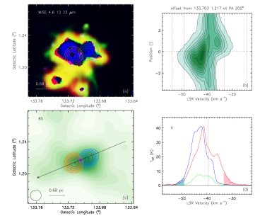
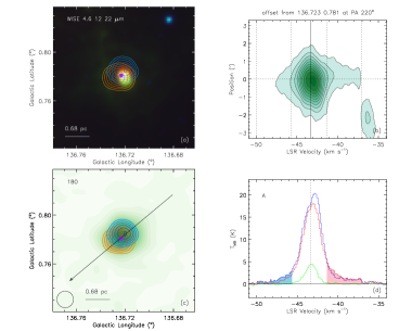
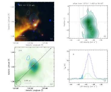
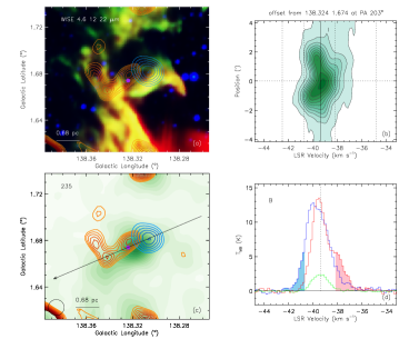
Figure 1: Four example outflow candidates with indexes 85, 180, 214, 235 (see the indexes in panel (c) for each). (a): blue/red lobe contours superpose on WISE false color (blue, green and red for 4.6, 12 and 22 $\mu$m, respectively) image. (b): P-V diagram is along the black arrow (the position angle, PA, is reported at the top of the panel) which is shown in panel (c); the width to draw the P-V diagram is 1$\arcmin$ (2 pixels). (c): blue/red ¹²CO lobe contours overlay on the integrated intensity of ¹³CO cores depicted as green-filled contours. (d): the blue/red spectrum is the ¹²CO averaged over $3\times 3$ pixels centered at the blue/red emission peak positions, respectively; the green spectrum is the ¹³CO averaged over $3\times 3$ pixels centered at the purple point (denotes the position of outflow candidate) in panel (a) or (c); the blue/red line wing velocity range of each outflow candidate is specified with shading; the black dotted line in the center is of the peak velocity of ¹³CO. The physical scale or HPBW of ¹²CO is shown in the left-bottom corner of panels (a) or (c). The quality level of each outflow candidate is reported in the top left corner of panel (d).
(The complete figure set (459 images) is available in the online material.)

Table 2: The Outflow Candidates

Index	$l$	$b$	Blue Line Wing	Red Line Wing	Quality level	WISE Detection
	(°)	(°)	(km s-1)	(km s-1)	Blue$|$Red
the Perseus arm
1	130.136	-4.467	$(-44.3,-43.0)$	$\cdots$	B	?
2	130.155	-4.537	$(-44.6,-43.3)$	$\cdots$	B	Y
3	130.399	-0.728	$\cdots$	$(-29.8,-28.4)$	B	?
4	130.401	1.667	$\cdots$	$(-41.5,-40.4)$	C	Y
5	130.425	-0.831	$(-36.4,-34.9)$	$(-31.7,-29.7)$	C$|$C	Y
…

Note. — “Y” = Yes, “?” = Possible, “N” = No. For the quality levels, “A” denotes the most reliable outflow candidates which are typically high-velocity ones, “B” denotes reliable outflow candidates (which include the majority of the outflow candidates), and “C” denotes outflow candidates whose characteristics were not obvious. Outflow candidates with scores of “D” were removed from our sample, owing to their ambiguous outflow characteristics. For more details of the quality levels see Li et al. (2018).

(This table is available in its entirety in machine-readable form. A portion is shown here for guidance.)

Table 3: Outflow candidate Sample Statistics

Sub-region	Numbers of Outflow	Numbers of	Quality Level				WISE Detection
	Total(Blue$|$Red)	Bipolar Outflow	A	B	C		Y	?	N
Perseus arm	284(186$|$180)	82	41$|$14%	160$|$56%	83$|$29%		133$|$47%	136$|$48%	15$|$5%
Local arm	162(67$|$107)	12	10$|$6%	79$|$49%	73$|$45%		12$|$7%	87$|$54%	63$|$39%
Interarm 1	5(2$|$3)	0	3$|$60%	2$|$40%	0$|$0%		2$|$40%	3$|$50%	0$|$0%
Interarm 2	3(2$|$3)	2	2$|$67%	1$|$33%	0$|$0%		1$|$33%	2$|$67%	0$|$0%
Outer arm	5(5$|$4)	4	2$|$40%	2$|$40%	1$|$20%		5$|$100%	0$|$0%	0$|$0%
Total	459(262$|$297)	100	58$|$13%	244$|$53%	157$|$34%		153$|$33%	228$|$50%	78$|$17%

Note. — See Table 2 for the description of quality level and WISE detection. In addition, we present the numbers and percentages and separate them with a “$|$” for quality level and WISE detection.

Table 3 shows that the outflow candidates in the two interarm regions (interarms 1 and 2) contained only a minority of the total outflow candidates, indicating that star formation was primarily concentrated in the Galactic spiral arms. The quality level revealed that the interarm regions were excellent locations to study relatively isolated star formation. In addition, more bipolar outflow candidates were detected in the Perseus arm than in the Local arm. The outflow candidates in the Perseus arm also had a higher quality level and possessed a larger proportion of WISE associations than those in the Local arm. All these indicated that the Perseus arm contained more active star forming activities.

3.2 Comparison with W5 Complex CO (3 $\rightarrow$ 2) Outflow Surveys

There are a number of outflow studies toward the W3/4/5 complex, such as (e.g., Bretherton et al., 2002; Ginsburg et al., 2011; Zhu et al., 2011). Among these studies, Ginsburg et al. (2011) conducted a CO (3 $\rightarrow$ 2) outflow survey toward the entire W5 complex (a total of $\sim$ 3 deg² with $136\arcdeg.1\lesssim l\lesssim 138\arcdeg.7$ and $0\arcdeg.3\lesssim b\lesssim 2\arcdeg.0$) with data acquired at the 15 m James Clerk Maxwell Telescope (JCMT) using the HARP array, and they detected 40 outflows. We therefore compared our work with their survey. With a final map HPBW resolution of 18$\arcsec$ and RMS of $\sim$ 0.06 – 0.11 K at 0.42 km s^-1 channels, the sensitivity of the data used by Ginsburg et al. (2011) was superior to that considered in the current study (HPBW is 49$\arcsec$, RMS is 0.45 K in a $0.16$ km s^-1 channel). After comparing with the outflow detection in L1448 from Hatchell et al. (2007), Ginsburg et al. (2011) concluded that they were able to detect any outflow, but might count fewer lobes and it was also difficult to make flow-counterflow associations. Their results (see their figure 7) also showed that they might miss candidate outflow lobes by a factor of $\sim$ 2.

Figure 2 superposes the outflow survey of Ginsburg et al. (2011) to that from this work. Overall, the outflow candidates in this work shared a similar distribution to those in their survey, and 90% of the outflows in their survey were detected. The circles marked by “unmatched 1” and “unmatched 2” denote the unmatched regions, where “unmatched 1” corresponds to outflows 18 and 19, and “unmatched 2” to outflows 39 and 40, in their survey. The sizes of the major axis of these four outflows were less than 23$\arcsec$, which could be the likely reason for our failure to detect them. In addition, CO (3 $\rightarrow$ 2) lines require warmer temperatures for excitation ($E_{\nu}/k=33.2$ K above ground states) and may show higher detection rates in warmer regions than CO (1 $\rightarrow$ 0) lines (e.g., Takahashi et al., 2008; Curtis et al., 2010). One can consult figures 3 and 4 in Nakamura et al. (2011) as examples that demonstrate the difference between CO (1 $\rightarrow$ 0) and CO (3 $\rightarrow$ 2) outflows.

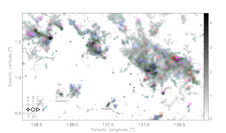
Figure 2: Outflow candidate distribution in the W5 complex. The background gray-scale map is the integrated intensity map of ¹²CO in the range of [-62, -30] km s^-1, the gray value is the square root of the integrated intensity, and the color bar is in units of (K km s^-1)^1/2. The green contours are the integrated intensity map of ¹³CO in the same velocity range as the ¹²CO map. Their levels are 10, 30, 60, 90, 120 $\times$ 0.58 K km s^-1 (1$\sigma$). The cyan contours denote ¹³CO emission boundaries, where the main beam brightness temperatures are larger than 3 $\times$ RMS in at least three successive channels. The blue/red open circles denote the blue/red lobes. The markers to describe quality level and classification of outflow candidates are placed in the bottom left corner of the panel, where 3, 2 and 1 denote high-, intermediate- and low-mass outflow candidates (see the criterion in Section 3.3), respectively. The magenta and red/blue colors of the shapes and the indexes denote bipolar outflow candidates and outflow candidates that have only a red/blue lobe, respectively. The diamonds represent the outflows found by Ginsburg et al. (2011). The brown circles denote the unmatched regions between (candidate) outflows in Ginsburg et al. (2011) and this work. The stars indicate OB stars (see the description in Section 4.1). The physical scale bar is reported in the bottom left corner of the panel.

There were many outflow candidates that were not reported in Ginsburg et al. (2011). One reason may be the difference between the CO (3 $\rightarrow$ 2) and (1 $\rightarrow$ 0) lines (see the panels (a) and (b) of Figure 3). The CO (3 $\rightarrow$ 2) presented a possible red high-velocity line wing while the CO (1 $\rightarrow$ 0) showed a blue one (e.g., Figure 1 and the panels (a) and (d) in Figure 3). Another reason may be that they were likely to miss many outflow candidates with large size (the mapped size in their studies was $\sim$ 2$\arcmin$) and/or in complex environments (e.g., the panel (d) in Figure 3). The CO (3 $\rightarrow$ 2) lines were likely to present more complex structures (e.g., Figure 1 and the panel (e) in Figure 3) or absent some structures (see an example close to the regions labeled by “EL 32” and “LFAM 36” in figures 3 and 4 in Nakamura et al., 2011) relative to CO (1 $\rightarrow$ 0) lines.

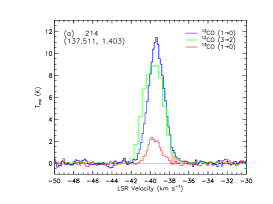
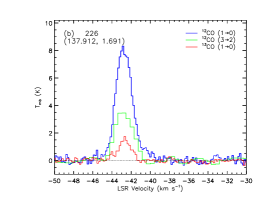
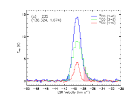
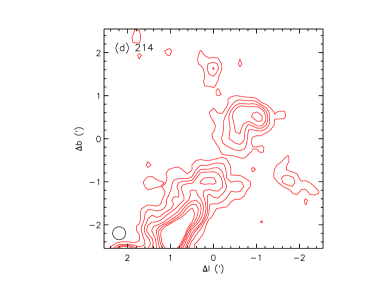
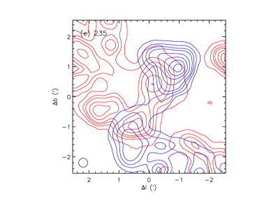
Figure 3: (a) – (c): mean spectra of ¹²CO (1 $\rightarrow$ 0), ¹²CO (3 $\rightarrow$ 2) and ¹³CO (1 $\rightarrow$ 0) averaged over $3\times 3$ pixels centered at the position shown in the spectra using Galactic coordinates. The possible velocity range of each high-velocity line wing of ¹²CO (3 $\rightarrow$ 2) is specified with shading. Indexes of outflow candidates in this work are reported in the top left corner of panels (a) – (e). (d) and (e): blue/red integrated intensity contours (integrated over the velocities indicated in upper panels with the same indexes) of the possible blue/red high-velocity line wings of ¹²CO (3 $\rightarrow$ 2). The contour levels are 0.5, 1, 1.5, 2, 3, 4, 5, 6 K km s^-1. The coordinate origin of panels (d) and (e) refers to the positions shown in panels (a) and (c), respectively. The circle in the lower left corner in panels (d) or (e) shows HPBW (18$\arcsec$) of ¹²CO (3 $\rightarrow$ 2) whose diameter is corresponding to $\sim 0.17$ pc with distance of $\sim$ 1960 pc.

3.3 Calculation of the Outflow Candidates’ Parameters

The area of an outflow lobe candidate, $A_{\mathrm{lobe}}$, is typically estimated by the contour that contains 40% of its peak integrated intensity. However, if an outflow candidate is contaminated by other components but can be resolved, $A_{\mathrm{lobe}}$ is estimated by the maximum area of the vicinity of the lobe where the outflow candidate’s components can be distinguished from the cloud. Owing to the limited capacity to resolve the detailed structures of an outflow candidate, the length of an outflow lobe candidate, $l_{\mathrm{lobe}}$, is estimated with an average collimation factor (2.45) derived by Wu et al. (2004) from 213 outflows. The collimation factor is defined as the ratio of the major and minor diameters (denoted them as $a$ and $b$, respectively, $a=2.45b$) of the region of an outflow lobe candidate. Therefore, $A_{\mathrm{lobe}}\sim\pi ab/4$ and $l_{\mathrm{lobe}}\sim a\sim 1.77\sqrt{A_{\mathrm{lobe}}}$.

The column density is estimated with ¹²CO assuming local thermal equilibrium (LTE), an area filling factor $f=1$, and optically thin line wings using $N(^{12}\mathrm{CO})=1.5\times 10^{15}\int{T_{\mathrm{mb}}}dv$ with $T_{ex}=30$ K (see Snell et al., 1984). If the ¹³CO emission is above the noise (i.e., $>$ RMS) over the line wing velocity range of the outflow lobe candidate, the correction factor for the opacity is $f_{\tau}=\tau_{12}/(1-e^{\tau_{12}})$ and $N(^{12}\mathrm{CO})$ is corrected to be $f_{\tau}N(^{12}\mathrm{CO})$, where $\tau_{12}$ is the optical depth of the ¹²CO line. In such a situation, $\tau_{12}$ can be calculated by multiplying $\tau_{13}$ (the optical depth of the ¹³CO line) by the abundance ratio, $[^{12}\mathrm{CO}]/[^{13}\mathrm{CO}]\sim 70$ (Milam et al., 2005) assuming that ¹²CO is optical thick, ¹³CO is optical thin, LTE, and identical filling factors (i.e., 1) and excitation temperatures (i.e., 30 K) for both isotopologues. The factor $\tau_{13}$ therein equals $-\ln(1-T^{13}_{\mathrm{mb}}/26.6)$ (for an excitation temperature of 30 K, Kawamura et al., 1998), where $T^{13}_{\mathrm{mb}}$ is the main beam brightness temperature of ¹³CO line. The total column density of an outflow lobe candidate of H₂ gas, $N_{\mathrm{lobe}}$, can be calculated by multiplying the corrected $N(^{12}\mathrm{CO})$ by a conversion factor $[\mathrm{H}]/[^{12}\mathrm{CO}]$ $=1\times 10^{4}$ (see e.g., Snell et al., 1984).

The mass of the outflow lobe candidate reads $M_{\mathrm{lobe}}=(N_{\mathrm{lobe}}\times A_{\mathrm{lobe}})m_{\mathrm{H_{2}}}$, where $m_{\mathrm{H_{2}}}$ is the mass of a hydrogen molecule. The momentum, $P_{\mathrm{lobe}}$, and kinetic energy, $E_{\mathrm{lobe}}$, of an outflow lobe candidate are based on the outflow candidate’s velocity relative to the central cloud (the lobe velocity, $\langle\Delta v_{\mathrm{lobe}}\rangle$). These physical parameters are

$$\langle\Delta v_{\mathrm{lobe}}\rangle=\frac{\sum_{i}\left(v_{i}-v_{\mathrm{peak}}\right)T_{i}\Delta v_{\mathrm{res}}}{\sum_{i}T_{i}\Delta v_{\mathrm{res}}},$$

$$\langle\Delta v^{2}_{\mathrm{lobe}}\rangle=\frac{\sum_{i}\left(v_{i}-v_{\mathrm{peak}}\right)^{2}T_{i}\Delta v_{\mathrm{res}}}{\sum_{i}T_{i}\Delta v_{\mathrm{res}}},$$

$$P_{\mathrm{lobe}}=\displaystyle\sum_{A_{\mathrm{lobe}}}M_{\mathrm{lobe}}\langle\Delta v_{\mathrm{lobe}}\rangle,$$

$$E_{\mathrm{lobe}}=\frac{1}{2}\displaystyle\sum_{A_{\mathrm{lobe}}}M_{\mathrm{lobe}}\langle\Delta v^{2}_{\mathrm{lobe}}\rangle,$$

where $i$ and $T_{i}$ are the channel index of the blue/red wing and the main beam brightness temperature of each channel, respectively, and $\Delta v_{\mathrm{res}}$ is the velocity resolution of the channel.

The total mass, momentum and energy of the outflow lobe candidates in the W5 complex (see Figure 2) were $M_{\mathrm{tot}}\sim 72$ $M_{\sun}$, $P_{\mathrm{tot}}\sim 193$ $M_{\sun}$ km s^-1, and $E_{\mathrm{tot}}\sim 6\times 10^{45}$ erg. These values were much higher than those reported in Ginsburg et al. (2011) whose corresponding values were $\sim 1.5$ $M_{\sun}$, $\sim 10.9$ $M_{\sun}$ km s^-1, and $\sim 7\times 10^{44}$ erg, respectively. Considering only A-rated outflow candidates, the values were $\sim 18$ $M_{\sun}$, $\sim 61$ $M_{\sun}$ km s^-1, and $\sim 2\times 10^{45}$ erg, respectively. The mass, momentum and energy ratios between the A-rated outflow candidates in this work and those in their survey were $\sim$ 12, $\sim$ 6 and $\sim$ 3. These were similar to the mean ratios for the (candidate) outflows that both detected in this work and in their survey, where the selected relatively isolated outflow candidates were 180, 212, 213, 215 and 231 (corresponding to outflows 10, 16, 17, 20 and 25 in their survey, respectively). The specific value decreased from mass ratio to momentum ratio and from momentum ratio to energy ratio, likely implying that this work exhibited a bias towards detecting mass at lower velocities. Therefore the mass and momentum in this work was higher than those reported in Ginsburg et al. (2011) because lower-velocity gas was likely to dominate the column density in outflow lobes. Another reason for obtaining a higher mass and momentum in this work was possible that the outflows’ parameters reported in their work did not include optical depth correction for the CO (3 $\rightarrow$ 2) lines (the correction factor ranged from 1.8 to 14.3, Curtis et al., 2010).

The dynamical timescale of an outflow lobe candidate is measured by $t_{\mathrm{lobe}}=l_{\mathrm{lobe}}/\Delta v_{\mathrm{max}}$, where $\Delta v_{\mathrm{max}}$ is the maximum velocity of an outflow lobe candidate (similar to Beuther et al., 2002) which is based on the sensitivity of our data, i.e., 0.45 K per 61 kHz channel for ¹²CO. The luminosity of an outflow lobe candidate is then $L_{\mathrm{lobe}}=E_{\mathrm{lobe}}/t_{\mathrm{lobe}}$. The physical properties of the outflow candidates in the Perseus arm, the Local arm and interarm 1 are listed in Table 4. Outflow candidates in interarm 2 and the Outer arm are not included in the table because they are highly clustered and hence causes large errors in $A_{\mathrm{lobe}}$ and other related physical parameters (see more details in Li et al., 2018).

Table 4: Physical Properties of the Outflow Candidate Samples

Index	Lobe	$l$	$b$	$v_{\mathrm{c}}$	$\langle\Delta v_{\mathrm{lobe}}\rangle$	$l_{\mathrm{lobe}}$	$M_{\mathrm{lobe}}$	$P_{\mathrm{lobe}}$	$E_{\mathrm{lobe}}$	$t_{\mathrm{lobe}}$	$L_{\mathrm{lobe}}$
		($\arcdeg$)	($\arcdeg$)	(km s-1)	(km s-1)	(pc)	($M_{\odot}$)	($M_{\odot}$ km s-1)	(1043 erg)	(105 yr)	(1030 erg s-1)
the Perseus arm
1	Blue	130.136	-4.467	-41.68	2.10	1.56	0.23	0.49	1.02	5.82	0.55
2	Blue	130.155	-4.537	-42.65	1.43	1.98	0.36	0.51	0.72	9.94	0.23
3	Red	130.399	-0.728	-31.84	2.60	1.87	0.60	1.55	4.01	5.30	2.40
4	Red	130.401	1.667	-42.86	1.80	0.95	0.05	0.09	0.16	3.79	0.14
5	Blue	130.417	-0.842	-33.79	2.01	1.53	0.31	0.62	1.23	5.74	0.68
	Red	130.433	-0.819	-33.34	2.44	5.65	9.22	22.50	54.20	15.20	11.30
…

Note. — $v_{\mathrm{c}}$ denotes the center velocity of ¹³CO for an outflow lobe candidate.

(This table is available in its entirety in machine-readable form. A portion is shown here for guidance.)

In addition to the opacity, inclination and blending can also affect the derived outflow parameters (Arce & Goodman, 2001). Inclination effects can greatly reduce the amount of $l_{\mathrm{lobe}}$, $\langle\Delta v_{\mathrm{lobe}}\rangle$, $P_{\mathrm{lobe}}$, $E_{\mathrm{lobe}}$, $t_{\mathrm{lobe}}$ and $L_{\mathrm{lobe}}$. Assuming a random distribution of inclination angles, the mean value is given by $\langle\theta\rangle=\int^{\pi/2}_{0}\theta\sin\theta d\theta=57\arcdeg.3$ (Bontemps et al., 1996; Dunham et al., 2014a). The blending effect can reduce the amount of $M_{\mathrm{lobe}}$ and other physical parameters related to $M_{\mathrm{lobe}}$ (e.g., $P_{\mathrm{lobe}}$, $E_{\mathrm{lobe}}$, and $L_{\mathrm{lobe}}$) by a factor of $\sim 2.0$, as previous studies have shown (Margulis & Lada, 1985; Arce et al., 2010; Narayanan et al., 2012). The effect that strong shocks dissociate molecular gas into atomic material only introduces a small error to the calculated mass and its related physical parameters, and it is equally true for the assumption of a single constant temperature (e.g., Downes & Ray, 1999; Downes & Cabrit, 2007; Curtis et al., 2010). For more information regarding the correction factors for the inclination and blending see the summary in table 5 of Li et al. (2018). Caution was taken that those corrections were only applied to statistics. We do not consider inclination or blending effects in this work except where otherwise noted.

The outflow candidates were classified as high-, intermediate- and low-mass for the Perseus arm, the Local arm and interarm 1 using the mass criteria of Yang et al. (2018). An outflow candidate was classified as high-mass if the corrected mass for any one lobe was greater than 5 $M_{\sun}$. An intermediate-mass classification was given to candidates whose corrected mass ranged from 0.5 – 5 $M_{\sun}$, while a low-mass designation was assigned to the rest.

3.4 The Limitations of the Survey

Because of the sensitivity of 0.45 K per 61 kHz channel (corresponding to $\sim$ 0.16 km s^-1 at 115.271 GHz) and moderate HPBW of 49$\arcsec$ for ¹²CO, some outflows with faint emissions, low velocities, complex environments or small sizes could be missed. Some clustered outflows might be presented as extended lobes because of poor resolution and might be omitted. The identified outflow candidates might actually be multi-outflows owing to the moderate resolution, or highly clustered in regions with distance $\gtrsim$ 3.8 kpc(see Section 3.3). Some outflow candidates were regarded as monopolar because their counterflows could be too faint/confused to be detected.

The total mass, momentum and energy of the outflow lobe candidates in the W5 complex (see Section 3.3) are $\sim$ 2 – 3 times higher than those in the Perseus molecular cloud complex (their corresponding parameters were $\sim$ 26 $M_{\sun}$, $\sim$ 60 $M_{\sun}$ km s^-1, and $\sim$ 2 $\times$ $10^{45}$ erg, see Arce et al., 2010). The (candidate) outflow mass ratio between those in W5 and those in the Perseus molecular cloud complex (i.e., $\sim$ 2 – 3) was less than their corresponding gas mass ratio (i.e., $\sim$ 3 – 5, Bally et al., 2008; Ginsburg et al., 2011). Two factors might be responsible for the deficiency of the mass, momentum and energy of the outflow candidates: a greater fraction of the outflow mass was blended with the cloud in the more turbulent W5 region (Ginsburg et al., 2011), and/or the limiting mass, momentum and energy of the outflow candidates in the Perseus arm were higher than those in the Perseus molecular cloud complex.

Figure 4 shows the physical parameters of the candidates in the Perseus arm, the Local arm and interarm 1. The lobe candidate velocity, $\langle\Delta v_{\mathrm{lobe}}\rangle$, was less than the extensional velocity of a minimum velocity extent relative to the ambient gas. We saw a $\langle\Delta v_{\mathrm{lobe}}\rangle$ that was lower than 1.0 km s^-1 for some sample points in panel (b). In panel (c), because the main beam brightness temperatures in some channels were less than 3 $\times$ RMS over the line wing velocity range of the outflow lobe candidates, we saw smaller candidate lobe mass ($M_{\mathrm{lobe}}$) than the limiting mass for some sample points. $\langle\Delta v_{\mathrm{lobe}}\rangle$ was less affected by distance effect.

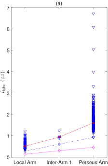
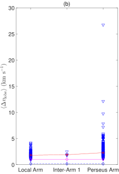
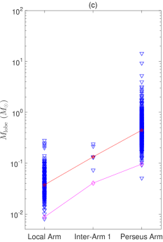
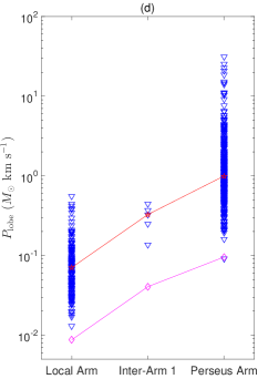
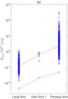
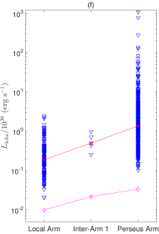
Figure 4: Physical parameters of the candidate outflow lobes in Perseus arm, the Local arm and the interarm 1. The red lines and open pentagrams show the median values for all panels. (a) The lengths of the candidate outflow lobes, where the purple and blue line/diamonds denote the HPBW of ¹²CO and three pixel sizes, respectively. (b) The velocities of the candidate outflow lobes, where the dash line shows the velocity resolution (0.16 km s^-1) for ¹²CO, and the purple line indicates 1.0 km s^-1, which refers to the threshold of the extensional velocity for a minimum velocity extent relative to the ambient gas (see Li et al., 2018). (c)–(f): The mass, momentum, energy and luminosity, respectively, of the candidate outflow lobes. The purple lines and diamonds denote the sensitivities of this work, where the HPBW, the velocity of candidate outflow lobe (1.0 km s^-1) and a main beam brightness temperature of 3 $\times$ RMS were used to calculate the sensitivities.

From Figure 4, the length, mass, momentum, energy and luminosity of the majority of the outflow lobe candidates in the Perseus arm were much greater than those in the other two regions (the Local arm and interarm 1). This implied that the amount of outflow missed in the Perseus arm was larger than those in the other two regions (i.e., we were more likely to see outflow clusters as single candidates).

Now we will discuss how many outflows we may have missed. From Figure 2, there are seven CO (3 $\rightarrow$ 2) outflows (26 – 32, from a total of 8 blue/red lobes, Ginsburg et al., 2011) near the densest region of the W5 complex, the bipolar outflow candidate 233. Combining the fact that Ginsburg et al. (2011) might have missed candidate outflow lobes by a factor of $\sim 2$ (see Section 3.2), we may have missed possible outflow lobes by a factor (scale-up factor, SUF, see Li et al., 2018) of $\lesssim$ 8 in the Perseus arm. This value is similar to the SUFs used for the Gem OB1 molecular cloud complex, where a different method was applied by comparing the outflow column densities $N_{\mathrm{o}}$ (Li et al., 2018). It is expected that the SUFs for the Local arm and interarm 1 were also $\lesssim$ 8 (see above). In addition, because $N_{\mathrm{o}}$ in the Local arm was $\sim$ 6 times higher than that in the Perseus arm, the SUF in the Local arm was probably less than $\sim$ 2.

4 The Spatial Distribution of The Outflow Candidates

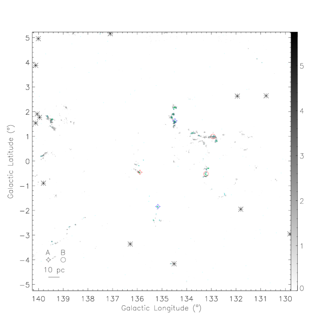
Figure 9: Outflow candidate distribution in the interarm 1. The background gray-scale map is the integrated intensity map of ¹²CO in the range of [-30, -20] km s^-1, the gray value is the square root of the integrated intensity, and the color bar is in units of (K km s^-1)^1/2. The green contours are the integrated intensity map of ¹³CO in the same velocity range as the ¹²CO map. They start at 5$\sigma$ with $\sigma=0.33$ K km s^-1, and the contour interval is 20% of the difference between the peak intensity and 5$\sigma$. The cyan contour denotes ¹³CO emission boundaries, where the main beam brightness temperatures are larger than 3 $\times$ RMS in at least three successive channels. The markers to describe quality level of outflow candidates is placed in the bottom left corner of the panel. The red/blue color of the shapes denote outflow candidates that have only a red/blue lobe, respectively. All the outflow candidates are low-mass ones (see the Section 3.3). The stars indicate OB stars. The physical scale bar is reported in the bottom left corner of the panel.

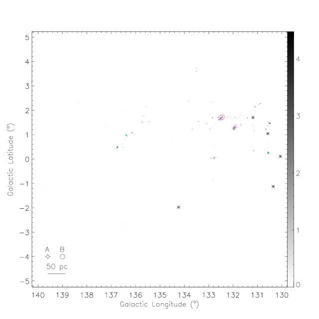
Figure 10: Outflow candidate distribution in the interarm 2. The background gray-scale map is the integrated intensity map of ¹²CO in the range of [-68, -62] km s^-1, the gray value is the square root of the integrated intensity, and the color bar is in units of (K km s^-1)^1/2. The green contours are the integrated intensity map of ¹³COin the same velocity range as the ¹²CO map. They start at 5$\sigma$ with $\sigma=0.25$ K km s^-1, and the contour interval is 20% of the difference between the peak intensity and 5$\sigma$. The cyan contours denote ¹³CO emission boundaries, where the main beam brightness temperatures are larger than 3 $\times$ RMS in at least three successive channels. The markers to describe quality level of outflow candidates is placed in the bottom left corner of the panel. The magenta and red colors of the shapes denote bipolar outflow candidates and outflow candidates that have only a red lobe, respectively. The stars indicate OB stars. The physical scale bar is reported in the bottom left corner of the panel.

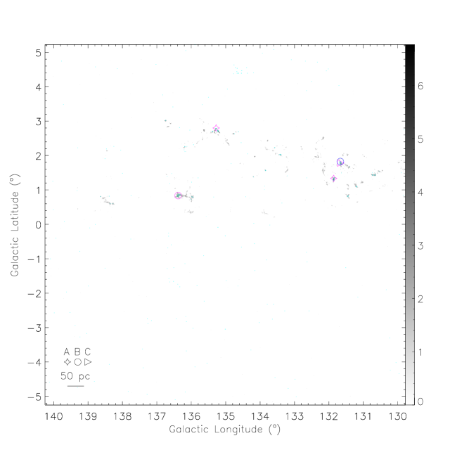
Figure 11: Outflow candidate distribution in the Outer arm. The background gray-scale map is the integrated intensity map of ¹²CO in the range of [-88, -68] km s^-1, the gray value is the square root of the integrated intensity, and the color bar is in units of (K km s^-1)^1/2. The green contours are the integrated intensity map of ¹³CO in the same velocity range as the ¹²CO map. They start at 5$\sigma$ with $\sigma=0.46$ K km s^-1, and the contour interval is 20% of the difference between the peak intensity and 5$\sigma$. The cyan contours denote ¹³CO emission boundaries, where the main beam brightness temperatures are larger than 3 $\times$ RMS in at least three successive channels. The markers to describe quality level of outflow candidates is placed in the bottom left corner of the panel. The magenta and blue colors of the shapes denote bipolar outflow candidates and outflow candidates that have only a blue lobe, respectively. The physical scale bar is reported in the bottom left corner of the panel.

In this section the spatial distribution of the outflow candidates in each arm or inter-arm region are described. Further steps were subsequently made to present close-up views of interesting active regions (IARs hereafter) in the W3/4/5 complex. The maps are shown in Figures 2 and 5 – 11.

4.1 The Perseus Arm — the W3/4/5 Complex

Figure 5 shows the spatial distribution of the outflow candidates in the Perseus arm. The OB stars (Xu et al., 2018, and references therein) are marked by stars in Figures 2 and 5 – 10. Most outflow candidates were located at the rectangles marked in Figure 5, where the red one indicates the W5 complex that was magnified in Figure 2. The detailed distribution of the outflow candidates in these IARs is discussed in the following subsections.

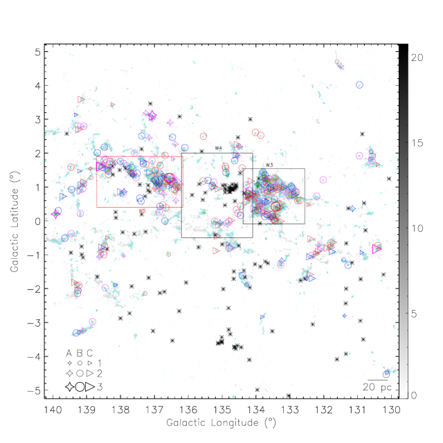
Figure 5: Outflow candidate distribution in the Perseus arm. The background gray-scale map is the integrated intensity map of ¹²CO in the range of [-62, -30] km s^-1, the gray value is the square root of the integrated intensity, and the color bar is in units of (K km s^-1)^1/2. The green contours are the integrated intensity map of ¹³CO in the same velocity range as the ¹²CO map. Their levels are 10, 30, 60, 90 120 $\times$ 0.58 K km s^-1 (1$\sigma$). The cyan contours denote ¹³CO emission boundaries, where the main beam brightness temperatures are larger than 3 $\times$ RMS in at least three successive channels. The blue/red open circles denote the blue/red lobes. The markers to describe quality level and classification of outflow candidates is placed in the bottom left corner of the panel, where 3, 2 and 1 denote high-, intermediate- and low-mass outflow candidates, respectively. The magenta, red/blue colors of the shapes denote bipolar outflow candidates and outflow candidates that have only a red/blue lobe, respectively. The stars indicate OB stars. The physical scale bar is reported in the bottom right corner of the panel. The rectangles denote IARs.

4.1.1 W5 Complex

Ginsburg et al. (2011) divided the W5 complex into eight sub-regions to analyze the outflows’ properties (see figure 3 and section 4 in their paper). It is convenient to describe CO (1 $\rightarrow$ 0) outflow candidates in Figure 2 (the eight individual regions are not marked in the figure to avoid complicating the map) based on these sub-regions.

Outflow candidates in S201. This region contains outflow candidates 247, 248, 250 (a high-mass one) and 253. Here the star-forming process was not affected by the HII region Sh 2-201 or by radiation-driven shocks from the nearest W5 O-stars (Ginsburg et al., 2011).

Outflow candidates in LWCas. A ridge separated the W5 complex into two HII region bubbles (i.e., HII regions W5-E and W5-W; Deharveng et al., 2012). This region contained outflow candidates 214, 215, and 217 – 222. The consistence of the CO (1 $\rightarrow$ 0) and (3 $\rightarrow$ 2) outflow candidates (20 from Ginsburg et al., 2011, and 215 from this work) went a step further to confirm this outflow. This region thus provided candidates for radiation-driven implosion and for investigating the relationship between HII regions and a new generation of star formation. As stated by Ginsburg et al. (2011), this region could serve as an example to explore the transition from molecular to atomic gas under the influence of ionizing radiation regions.

Outflow candidates in W5S (containing outflow candidates 212 and 213). Three cometary clouds in W5S have been pushed in different directions by the HII region IC 1396 (Ginsburg et al., 2011; Huang et al., 2013). Protostars driving the candidate outflows in these cometary clouds were probably triggered by the radiation-driven implosion mechanism (e.g., Ginsburg et al., 2011).

Outflow candidates in W5SW. Outflow candidate 180 was associated with an isolated clump that showed little evidence of interaction with the HII region (similar to outflow 10 from Ginsburg et al., 2011).

Outflow candidates in W5NW. This region contained outflow candidates 163, 166, 169, 171, 172, 174, 178 and 181, and therefore contained actively forming stars. Similar to the conclusion of Ginsburg et al. (2011), this region has not been directly impacted by W5 O-stars.

Outflow candidates in other regions in the W5 complex. Outflow candidates 221, 223, 226 and 229 surrounded the east HII region bubble relative to the W5 ridge (i.e., HII region W5-E, Deharveng et al., 2012) which was excited by the double or multiple star HD 18326 (see also the star marked in Figure 2, Chauhan et al., 2011; Deharveng et al., 2012; Gaia Collaboration et al., 2018) whose spectral type was O6.5V+O9/B0V (Sota et al., 2014). This implied that these candidates might be affected by the HII region W5-E.

4.1.2 W4 Complex

The expanding superbubble/HII region W4 was suggested as being driven by the open cluster IC 1805 (centered at the W4 complex; Basu et al., 1999; Lagrois & Joncas, 2009). A total of 126 stars were intrinsic to the open cluster, where the presence of numerous massive stars has been confirmed (about 40 from spectral types O4 to B2, see the OB stars in Figures 5 – 6, and Shi & Hu, 1999; Reed, 2003; Lagrois & Joncas, 2009). However, this region showed very few CO clouds, which were mainly concentrated to the east of this open cluster as well as in a shell-like structure with a radius of $\sim$ 35 pc (see Figure 6 and Lagrois & Joncas, 2009).

Overall, CO outflow activities in the W4 complex are much fewer than that in the W3 (see below) and W5 complexes. One reason may be that the CO gas was collapsed by UV photons from the OB association IC 1805. Outflow candidates 138 – 140 were located in a cometary cloud in the north of this region. The HII region W4 was probably responsible for impacting or even triggering the formation of the driving protostars of these three outflow candidates. In the southern region, CO emission in a thin shell (see above) with a width of $\lesssim$ 1 pc was concentrated on the north side (i.e., toward the HII region). The formation of the driving protostars of the ten outflow candidates located at this thin shell were probably impacted by the interaction between the HII regions and the surrounding clouds. Outflow candidates 143 and 147 – 149 were close to elephant-trunk-like structures (extracted from homogeneous infrared data-sets obtained by the 2MASS, GLIMPSE, MIPS and WISE surveys) in which the star formation therein was possibly due to a triggering effect caused by the expanding W4 bubble (Panwar et al., 2019). It was difficult to understand the outflow candidates in the eastern part of the HII region (i.e., 150 and 152). They were weak and could be radiation-driven flows.

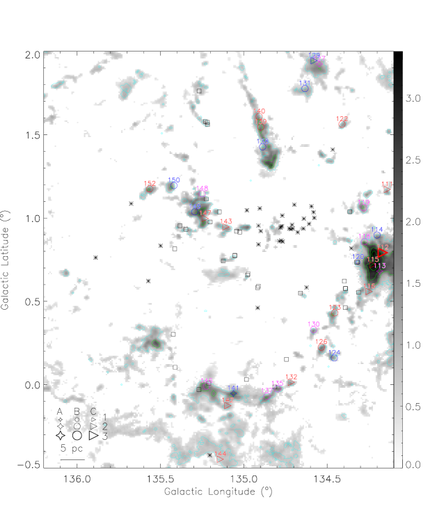
Figure 6: Outflow candidate distribution in W4 complex. The description refers to Figure 5. The blue/red numbers are the indexes of the outflow candidates that have only a blue/red lobe, and the magenta numbers mark the bipolar outflow candidates. The squares present elephant trunk-like structures in which the star formation is going on possibly due to triggering effect of expanding W4 bubble (Panwar et al., 2019).

4.1.3 W3 Complex

The W3 complex is a smaller relative to the W4 and W5 complexes, and is on the western edge of the W4 shell (see Figure 5 and Oey et al., 2005). W3 North, W3 Main, W3(OH), W3(H₂O) and AFGL 333 consist of a ridge that forms a boundary between the W3 and W4 complexes (Oey et al., 2005; Rivera-Ingraham et al., 2011).

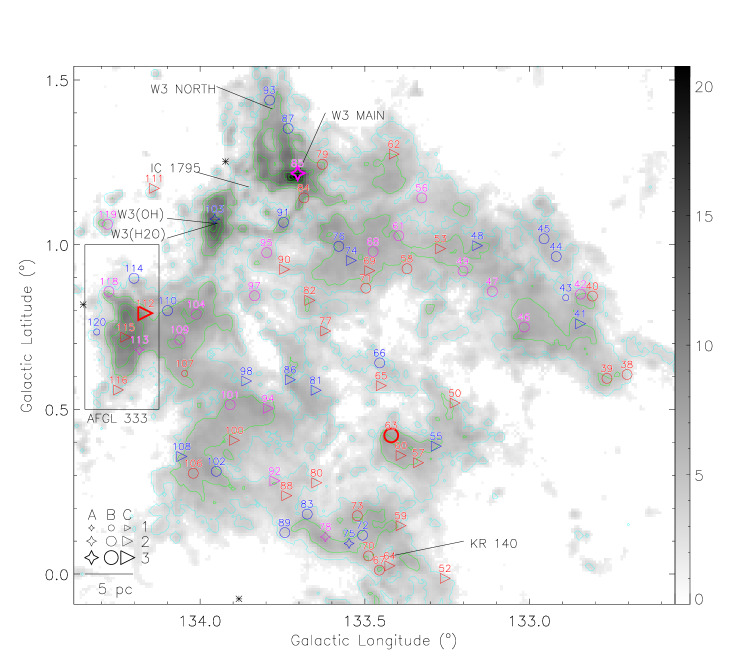
Figure 7: Outflow candidate distribution in W3 complex. The description refers to Figure 5. The blue/red numbers are the indexes of the outflow candidates that have only a blue/red lobe, and the magenta numbers mark the bipolar outflow candidates.

Overall, the W3 complex showed much more active star formation in the view of outflow activities relative to the W5 and W4 complexes, i.e., the outflow column density (see e.g., Li et al., 2018) in the W3 complex ($\sim$ 0.021 pc^-2) was larger than that in the W5 complex ($\sim$ 0.016 pc^-2) and in the W4 complex ($\lesssim$ 0.006 pc^-2). Most of the high-mass outflow candidates were located in the IARs, such as outflow candidates 112 in AFGL 333 and 85 in W3 Main. Outflow candidates for each IARs are described as follows:

In AFGL 333, outflow candidate 115 was associated with an outflow identified from the CO (2 $\rightarrow$ 1) line and an H₂O maser (see Nakano et al., 2017). They also suggested that star formation in the AFGL 333 region proceeded without significant external triggers.

Hosting a bright O6.5V star, an O9.7I star and two B stars (Mathys, 1989; Oey et al., 2005), the IC 1795 cluster ionized a diffuse HII region G133.71+1.21 in the W3 complex (Wink et al., 1983; Roccatagliata et al., 2011). This region contained several sites of high- and low-mass star formations: W3(OH), W3 Main, and W3 North (Oey et al., 2005; Roccatagliata et al., 2011).

The W3(OH) complex, which contained W3(OH) itself and W3(H₂O), was a well-studied high-mass star forming region (Qin et al., 2016). The only outflow candidate, 103, was associated with CO (2 $\rightarrow$ 1) outflows (Zapata et al., 2011) and HCN outflows detected by Qin et al. (2016). A sketch of the dynamical state of the W3(OH) star forming complex can be found in Figure 8 of Qin et al. (2016).

W3 Main is an ideal region to simultaneously investigate massive star formation at different evolutionary stages (Wang et al., 2012). High-mass outflow candidate 85 was located in the midst of outflows W3 SMS1 and W3 SMS2 (see figures 11 and 13 in Wang et al., 2012, respectively). Triggered star formation may be responsible for this outflow, because evidence for interactions between the molecular cloud and the HII regions has been found in the W3 Main complex (such as the ultracompact HII regions W3 C and W3 F; see Wang et al., 2012, and references therein).

The bright HII region W3 North (G133.8+1.4) was less well studied than those mentioned above. An O6 star was detected at ($02^{\mathrm{h}}26^{\mathrm{m}}49.62^{\mathrm{s}},+62\arcdeg 15\arcmin 35.0\arcsec$)(J2000) via Chandra observations (Feigelson & Townsley, 2008). Because of its small size of $\sim 5\arcmin$ (Quireza et al., 2006), it was difficult to see a shell-like structure even if it has one. The nearest outflow candidate, 93, is $\sim 2\arcmin$ to the north of this HII region. This outflow candidate may be impacted by the HII region W3 North.

The HII region KR 140, powered by an O star Ves 735 (Kerton et al., 1999), has been investigated in multi-wavelength sub-mm (include 450 and 850 $\mu$m) studies (Ballantyne et al., 2000; Kerton et al., 2001). Kerton et al. (2001) detected numerous sub-mm dust cores located at the interface between the ionized and molecular gas, likely implying that the star formation was impacted by the expansion of the HII region. Outflow candidates 59, 64, 70, and 72 were located in a shell-like structure with a diameter of $\sim$ 5 pc that surrounded HII region KR 140 (consistent with the size of this HII region, see Kerton et al., 2008). They shared a similar distribution of sub-mm dust cores seen by Kerton et al. (2001), which indicated that these outflow candidates were probably impacted by the expansion of the HII region.

The outflow candidates in the other regions were well distributed in the shell-like structure of the superbubble/HII region W3 with a radius of $\sim$ 13 pc for the inner side. They were likely to be impacted by the HII region W3. It was noticeable that outflow candidates were distributed nearly uniformly across the field. Such distribution was probably real at least in current angular resolution, because such distribution was obeyed by both B-rated and C-rated outflow candidates (there were only five A-rated outflow candidates) but did not appear in the W4 (Figure 6) and W5 (Figure 2) cloud complex and in the entire Perseus arm regions (Figure 5).

4.1.4 Other Regions in the Perseus Arm

Some outflow candidates also surrounded OB stars in other regions in the Perseus arm. For example, to the south of the W5 complex, with a projected distance to the boundary of the W5 complex of $\sim$ 42 pc, eight outflow candidates were located in a shell-like cloud (radius is $\sim$ 10 pc) which surrounded the B2III star ALS 7530 (centered at $(l,b)=(138\arcdeg.394,-0\arcdeg.834)$ at a distance of $\sim 2088$ pc, Rydstrom, 1978; Reed, 2003; Gaia Collaboration et al., 2016). These outflow candidates were likely impacted by the OB stars.

A small number of outflow candidates were located far from OB stars, indicating that they were untriggered (spontaneous). Overall, the studied regions in the Perseus arm, especially the W3 complex, contained massive stars at various evolutionary stages (e.g., Tieftrunk et al., 1997). This region, especially in the eastern HDL in the W3 complex that neighbors the W4 complex (see the eastern part of Figure 7), contained the most active star-forming sites with signatures of massive star formation in a triggered environment (Oey et al., 2005).

4.2 The Local Arm

Some outflow candidates, including the the only two intermediate-mass ones, were located in shell-like regions (IARs, see the five rectangles marked in Figure 8). Four outflow candidates were located in a shell-like region (radius of the shell is $\sim 3$ pc) which surrounded an open cluster, Cl Stock 2 with an age of 300 Myr ($l$ = 133.°33, $b$ = 1.°69, Kharchenko et al., 2013; Schmeja et al., 2014; Scholz et al., 2015). Surrounding the shell-like structure in the other four IARs (mark by rectangles and labelled as regions II – V) with radii of approximately 5, 4, 3, and 4 pc, we detected 10 (include an intermediate-mass one), 3, 6 and 8 (include an intermediate-mass one) outflow candidates, respectively. Eight weak OB stars were found to be close to the center of these four IARs in SIMBAD:

1. For region II they were B9V star TYC 3699-871-1 (Høg et al., 2000; Cutri et al., 2003; Gaia Collaboration et al., 2016), at a distance of $\sim$ 700 pc and located at ($l,b$) $\sim$ (134$\arcdeg$.8, -0$\arcdeg$.6), and B8/B9 star GSC 03699-00325 (Morrison et al., 2001; Cutri et al., 2003; Gaia Collaboration et al., 2016) with a distance of $\sim$ 600 pc located at ($l,b$) $\sim$ (135$\arcdeg$.2, -0$\arcdeg$.6);

2. For region III they were B1 star GSC 0369-02027 (Morrison et al., 2001; Cutri et al., 2003; Gaia Collaboration et al., 2016) located at ($l,b$) $\sim$ (136$\arcdeg$.5, -1$\arcdeg$.1) and B9V star HD 15979 (Nesterov et al., 1995; Cutri et al., 2003; Gaia Collaboration et al., 2016) located at ($l,b$) $\sim$ (136$\arcdeg$.1, -1$\arcdeg$.1) with a distance of $\sim$ 500 pc;

3. For region IV they were B9V star HD 16025 located at ($l,b$) $\sim$ (136$\arcdeg$.5, -2$\arcdeg$.0) and B9 III star HD 16494 located at ($l,b$) $\sim$ (137$\arcdeg$.1, -2$\arcdeg$.0) with a distance of $\sim$ 500 pc (Nesterov et al., 1995; Cutri et al., 2003; Gaia Collaboration et al., 2016);

4. And for region V they were B9 star TYC 3714-344-1 (Høg et al., 2000; Cutri et al., 2003; Gaia Collaboration et al., 2016) located at ($l,b$) $\sim$ (139$\arcdeg$.7, 1$\arcdeg$.4) with a distance of 800 pc and B8 II-III star V^∗ V368 (Kukarkin et al., 1971; Morrison et al., 2001; Gaia Collaboration et al., 2016) located at ($l,b$) $\sim$ (139$\arcdeg$.8, 1$\arcdeg$.7) with a distance of $\sim$ 900 pc.

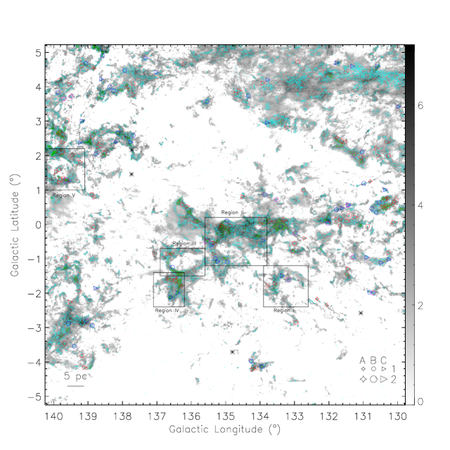
Figure 8: Outflow candidate distribution in the Local arm. The background gray-scale map is the integrated intensity map of ¹²CO in the range of [-20, 7] km s^-1, the gray value is the square root of the integrated intensity, and the color bar is in units of (K km s^-1)^1/2. The green contours are the integrated intensity map of ¹³CO in the same velocity range as the ¹²CO map. They start at 5$\sigma$ with $\sigma=0.55$ K km s^-1, and the contour interval is 20% of the difference between the peak intensity and 5$\sigma$. The cyan contours denote ¹³CO emission boundaries, where the main beam brightness temperatures are larger than 3 $\times$ RMS in at least three successive channels. The markers to describe quality level and classification of outflow candidates is placed in the bottom right corner of the panel, where 2 and 1 denote intermediate- and low-mass outflow candidates (see the criterion in Section 3.3), respectively. The magenta, red/blue colors of the shapes denote bipolar outflow candidates and outflow candidates that have only a red/blue lobe, respectively. The stars indicate OB stars. The physical scale bar is reported in the bottom left corner of the panel. The rectangles denote IARs.

For region III, the bubble size of the B1 star is $\sim$ 3 – 8 pc (Chen et al., 2013), and the typical radius of the HII regions was $\sim$ 5 pc (Quireza et al., 2006). They are approximated to the radius of the four shell-like structures. If the association among the stars and the shell-like structures is confirmed by future studies, these five IARs could be candidates to study the impact on star formation imposed by massive or intermediate-mass stars.

4.3 Other Regions

CO clouds in the Outer arm are much rarer than those in the Perseus arm and the Local arm, but were more crowded than those in interarm 1 and interarm 2. The outflow candidates were distributed in these rare CO clouds in the Outer arm, interarm 1 and interarm 2.

In interarm 1, all the outflow candidates were low-mass. The southernmost outflow candidate (index is 450) was located in a relatively isolated cloud, which might be a great example to investigate star formation. The other four outflow candidates were located in filamentary structures that had little mixture to ambient gas.

Because their distances were $\gtrsim$ 4 kpc, the outflow candidates in interarm 2 and the Outer arm were highly clustered (see Section 3.3), and their physical parameters are not reported here. We detected two candidate (bulk) outflows (the north ones) in a filamentary-like cloud with a length of dozens of pc in interarm 2.

All the candidate (bulk) outflows in the Outer arm were located in filamentary structures with lengths of dozens of pc. The northernmost and the southernmost filamentary structures, especially the former, showed a heavy head or tail, which was evidence for interactions with external forces such as those driven by high- or intermediate-mass stars. For example, the ultracompact HII region IRAS 02395+6244 with ($l,b$) = (135$\arcdeg$.278, 2$\arcdeg$.797) and $V_{\mathrm{lsr}}$ = -71.5 km s^-1 (Bronfman et al., 1996; Yan et al., 2018), was probably an indicator of such a driven source.

5 Discussion

5.1 Star Formation Activity

CO (1 $\rightarrow$ 0) outflow candidates were used to evaluate star formation in this work. Because a protostar outflow is a common phenomenon for star formation in the stage of Class 0 and I (e.g., Bachiller, 1996; Bally, 2016), we will compare outflow candidates with class 0/I sources in the following discussion.

Koenig et al. (2008) detected 171 Class I sources in the W5 complex and Rivera-Ingraham et al. (2011) detected 184 Class 0/I and 560 Class 0/I^∗ (highly embedded YSOs) sources in W3 Main/(OH), KR 140 and AFGL 333, using Spitzer photometry. Outflows are nearly always associated with Class 0/I objects in nearby star-forming regions (e.g., Hatchell et al., 2007; Curtis et al., 2010). The low number of detected outflow candidates (284 in the Perseus arm, a region that contains W5, W3 Main/(OH), KR 140 and AFGL 333) can be explained as follows.

First, CO outflows were not detected in some Class I sources due to the removal or dissociation of CO gas by the protostar, such as in the HH34 complex (see Bally & Devine, 1994; Ginsburg et al., 2011; Bally, 2016). Optical or infrared jets can be used to test the association. Second, many outflow candidates were clusters of outflows rather than individual ones. For instance, there were a number of WISE spots located within the contours of the outflow candidate 152. Third, some outflows that exhibited faint emission, low velocity, complex environment, or small size could be missed.

We also detected some outflow candidates that did not have any WISE associations. These outflow candidates were probably driven by first hydrostatic cores, very young protostellar or proto-brown dwarfs, or driven by more evolved protostars with low accretion rates (Dunham et al., 2014b; Friesen et al., 2018). These sources may also be fake outflows. Because the Local arm contained a higher proportion of quantity level “C” candidates relative to other four regions, we might attribute the high percentage of “N” classifications (i.e. no WISE associations) for the Local arm in Table 4 to fake outflows or outflows with the abovementioned driven sources (for examples of outflows driven by candidates with the youngest protostars or first hydrostatic cores see Friesen et al., 2018). That is to say, outflow candidates with both “C” and “N” classifications( $\sim$ 20%, i.e., 33/162) were more likely to be fake outflows or outflows with the aforementioned driven sources.

5.2 Discussion of Triggering

The majority of the star formation in the W3/4/5 complex were likely impacted by their corresponding HII regions, although they may not be directly triggered by these HII regions. In the Local arm, star formation in the IARs marked in Figure 8 may be under the impact of massive or intermediate-mass stars. The outflow candidates in interarms 1 and 2 were far from OB stars, indicating that the star formation in these regions was probably untriggered (spontaneous). The OB stars were not shown in the Outer arm due to the large uncertainties in their calculated distances. Nevertheless, we still found that the formation of the driving protostars of the candidate (bulk) outflow (i.e., 458) in the Outer arm could be induced, triggered, or at least impacted by the HII region IRAS 02395+6244 (the projected distance between them was $\sim$ 0.4 pc, see Section 4.3). Infrared data, such as in the 5.8, 8.0, 12 and 24 $\mu$m bands (Watson et al., 2008; Deharveng et al., 2010; Yan et al., 2018), are helpful when studying HII regions in detail and are therefore advantageous for further investigations regarding induced or triggered star formation (traced by CO (1 $\rightarrow$ 0) outflow candidates) by HII regions.

6 Summaries

We conducted a large-scale survey of outflow features toward the W3/4/5 complex region (a total of $\sim$ 110 deg²) using ¹²CO and ¹³CO molecular lines. A set of semi-automated IDL scripts based on longitude-latitude-velocity space was used to search for and evaluate outflows over a large area. We detected 459 outflow candidates, of which 284 were in the Perseus arm, 162 in the Local arm, 5 in the Outer arm and the rest (i.e., 8) in interarm regions. Many of the identified outflow candidates were probably multi-outflow candidates resulting from the limited resolution, especially in regions at distances $\gtrsim$ 4 kpc.

As a summary, star formation was mainly concentrated to the Galactic spiral arms. The Perseus arm revealed more activities of stellar formation than those in the Local arm and other regions. There were still a few cases of star formation occurring in the interarm regions, and they were good examples to study relatively isolated star formation. The W3/4/5 complex in the Perseus arm, especially in the eastern HDL where the W3 complex neighbors the W4 complex, presented intense star formation activities. Most of the star formation in these complexes were likely impacted by the HII regions surrounding them.

References

- Adams & Fatuzzo (1996) Adams, F. C., & Fatuzzo, M. 1996, ApJ, 464, 256
- Araya et al. (2008) Araya, E., Hofner, P., Kurtz, S., Olmi, L., & Linz, H. 2008, ApJ, 675, 420
- Arce et al. (2010) Arce, H. G., Borkin, M. A., Goodman, A. A., Pineda, J. E., & Halle, M. W. 2010, ApJ, 715, 1170
- Arce & Goodman (2001) Arce, H. G., & Goodman, A. A. 2001, ApJ, 554, 132
- Arce et al. (2007) Arce, H. G., Shepherd, D., Gueth, F., et al. 2007, Protostars and Planets V, 245
- Bachiller (1996) Bachiller, R. 1996, ARA&A, 34, 111
- Ballantyne et al. (2000) Ballantyne, D. R., Kerton, C. R., & Martin, P. G. 2000, ApJ, 539, 283
- Bally (2016) Bally, J. 2016, ARA&A, 54, 491
- Bally & Devine (1994) Bally, J., & Devine, D. 1994, ApJ, 428, L65
- Bally et al. (2008) Bally, J., Walawender, J., Johnstone, D., Kirk, H., & Goodman, A. 2008, Handbook of Star Forming Regions, Volume I, 4, 308
- Basu et al. (1999) Basu, S., Johnstone, D., & Martin, P. G. 1999, ApJ, 516, 843
- Berry (2015) Berry, D. S. 2015, Astronomy and Computing, 10, 22
- Berry et al. (2007) Berry, D. S., Reinhold, K., Jenness, T., & Economou, F. 2007, Astronomical Data Analysis Software and Systems XVI, 376, 425
- Beuther et al. (2002) Beuther, H., Schilke, P., Sridharan, T. K., et al. 2002, A&A, 383, 892
- Bontemps et al. (1996) Bontemps, S., Andre, P., Terebey, S., & Cabrit, S. 1996, A&A, 311, 858
- Bretherton et al. (2002) Bretherton, D. E., Moore, T. J. T., & Ridge, N. A. 2002, Hot Star Workshop III: The Earliest Phases of Massive Star Birth, 267, 347
- Bronfman et al. (1996) Bronfman, L., Nyman, L.-A., & May, J. 1996, A&AS, 115, 81
- Cesaroni et al. (2011) Cesaroni, R., Beltrán, M. T., Zhang, Q., Beuther, H., & Fallscheer, C. 2011, A&A, 533, A73
- Chauhan et al. (2011) Chauhan, N., Pandey, A. K., Ogura, K., et al. 2011, MNRAS, 415, 1202
- Chen et al. (2013) Chen, Y., Zhou, P., & Chu, Y.-H. 2013, ApJ, 769, L16
- Curtis et al. (2010) Curtis, E. I., Richer, J. S., Swift, J. J., & Williams, J. P. 2010, MNRAS, 408, 1516
- Cutri et al. (2003) Cutri, R. M., Skrutskie, M. F., van Dyk, S., et al. 2003, VizieR Online Data Catalog, 2246
- Deharveng et al. (2010) Deharveng, L., Schuller, F., Anderson, L. D., et al. 2010, A&A, 523, A6
- Deharveng et al. (2012) Deharveng, L., Zavagno, A., Anderson, L. D., et al. 2012, A&A, 546, A74
- Deharveng et al. (1997) Deharveng, L., Zavagno, A., Cruz-Gonzalez, I., et al. 1997, A&A, 317, 459
- Downes & Cabrit (2007) Downes, T. P., & Cabrit, S. 2007, A&A, 471, 873
- Downes & Ray (1999) Downes, T. P., & Ray, T. P. 1999, A&A, 345, 977
- Dunham et al. (2014a) Dunham, M. M., Arce, H. G., Mardones, D., et al. 2014, ApJ, 783, 29
- Dunham et al. (2014b) Dunham, M. M., Vorobyov, E. I., & Arce, H. G. 2014, MNRAS, 444, 887
- Elmegreen (1998) Elmegreen, B. G. 1998, in ASP Conf. Ser. Vol. 148, Origins, ed. Charles E. Woodward, J. Michael Shull, and Harley A. Thronson, Jr. (San Francisco, CA: ASP), 150
- Feigelson & Townsley (2008) Feigelson, E. D., & Townsley, L. K. 2008, ApJ, 673, 354
- Fish & Sjouwerman (2007) Fish, V. L., & Sjouwerman, L. O. 2007, ApJ, 668, 331
- Frank et al. (2014) Frank, A., Ray, T. P., Cabrit, S., et al. 2014, in Protostars and Planets VI, ed. H. Beuther et al. (Tucson, AZ: Univ. Arizona Press), 451
- Friesen et al. (2018) Friesen, R. K., Pon, A., Bourke, T. L., et al. 2018, ApJ, 869, 158
- Gaia Collaboration et al. (2018) Gaia Collaboration, Brown, A. G. A., Vallenari, A., et al. 2018, A&A, 616, A1
- Gaia Collaboration et al. (2016) Gaia Collaboration, Prusti, T., de Bruijne, J. H. J., et al. 2016, A&A, 595, A1
- Ginsburg et al. (2011) Ginsburg, A., Bally, J., & Williams, J. P. 2011, MNRAS, 418, 2121
- Hatchell et al. (2007) Hatchell, J., Fuller, G. A., & Richer, J. S. 2007, A&A, 472, 187
- Høg et al. (2000) Høg, E., Fabricius, C., Makarov, V. V., et al. 2000, A&A, 355, L27
- Heyer & Terebey (1998) Heyer, M. H., & Terebey, S. 1998, ApJ, 502, 265
- Hirsch et al. (2012) Hirsch, L., Adams, J. D., Herter, T. L., et al. 2012, ApJ, 757, 113
- Huang et al. (2013) Huang, Y. F., Zeng Li, J., Rector, T. A., & Mallamaci, C. C. 2013, AJ, 145, 126
- Kawamura et al. (1998) Kawamura, A., Onishi, T., Yonekura, Y., et al. 1998, ApJS, 117, 387
- Kerton et al. (2008) Kerton, C. R., Arvidsson, K., Knee, L. B. G., & Brunt, C. 2008, MNRAS, 385, 995
- Kerton et al. (1999) Kerton, C. R., Ballantyne, D. R., & Martin, P. G. 1999, AJ, 117, 2485
- Kerton et al. (2001) Kerton, C. R., Martin, P. G., Johnstone, D., & Ballantyne, D. R. 2001, ApJ, 552, 601
- Kharchenko et al. (2013) Kharchenko, N. V., Piskunov, A. E., Schilbach, E., Röser, S., & Scholz, R.-D. 2013, A&A, 558, A53
- Koenig et al. (2008) Koenig, X. P., Allen, L. E., Gutermuth, R. A., et al. 2008, ApJ, 688, 1142
- Kukarkin et al. (1971) Kukarkin, B. V., Kholopov, P. N., Pskovsky, Y. P., et al. 1971, General Catalogue of Variable Stars, 3rd ed. (1971)
- Lagrois & Joncas (2009) Lagrois, D., & Joncas, G. 2009, ApJ, 691, 1109
- Li et al. (2015) Li, H., Li, D., Qian, L., et al. 2015, ApJS, 219, 20
- Li et al. (2018) Li, Y., Li, F.-C., Xu, Y., et al. 2018, ApJS, 235, 15
- Margulis & Lada (1985) Margulis, M., & Lada, C. J. 1985, ApJ, 299, 925
- Mathys (1989) Mathys, G. 1989, A&AS, 81, 237
- Morrison et al. (2001) Morrison, J. E., Röser, S., McLean, B., Bucciarelli, B., & Lasker, B. 2001, AJ, 121, 1752
- Moscadelli et al. (2013) Moscadelli, L., Li, J. J., Cesaroni, R., et al. 2013, A&A, 549, A12
- Moscadelli et al. (2016) Moscadelli, L., Sánchez-Monge, Á., Goddi, C., et al. 2016, A&A, 585, A71
- Moscadelli et al. (2010) Moscadelli, L., Xu, Y., & Chen, X. 2010, ApJ, 716, 1356
- Milam et al. (2005) Milam, S. N., Savage, C., Brewster, M. A., Ziurys, L. M., & Wyckoff, S. 2005, ApJ, 634, 1126
- Nakamura et al. (2011) Nakamura, F., Kamada, Y., Kamazaki, T., et al. 2011, ApJ, 726, 46
- Nakano et al. (2017) Nakano, M., Soejima, T., Chibueze, J. O., et al. 2017, PASJ, 69, 16
- Narayanan et al. (2012) Narayanan, G., Snell, R., & Bemis, A. 2012, MNRAS, 425, 2641
- Nesterov et al. (1995) Nesterov, V. V., Kuzmin, A. V., Ashimbaeva, N. T., et al. 1995, A&AS, 110, 367
- Norman & Silk (1980) Norman, C., & Silk, J. 1980, ApJ, 238, 158
- Oey et al. (2005) Oey, M. S., Watson, A. M., Kern, K., & Walth, G. L. 2005, AJ, 129, 393
- Panwar et al. (2019) Panwar, N., Samal, M. R., Pandey, A. K., Singh, H. P., & Sharma, S. 2019, AJ, 157, 112
- Peters et al. (2010) Peters, T., Banerjee, R., Klessen, R. S., et al. 2010, ApJ, 711, 1017
- Pety (2005) Pety, J. 2005, SF2A-2005: Semaine de l’Astrophysique Francaise, 721
- Qin et al. (2016) Qin, S.-L., Schilke, P., Wu, J., et al. 2016, MNRAS, 456, 2681
- Quireza et al. (2006) Quireza, C., Rood, R. T., Bania, T. M., Balser, D. S., & Maciel, W. J. 2006, ApJ, 653, 1226
- Reed (2003) Reed, B. C. 2003, AJ, 125, 2531
- Reid et al. (2014) Reid, M. J., Menten, K. M., Brunthaler, A., et al. 2014, ApJ, 783, 130
- Reid et al. (2009) Reid, M. J., Menten, K. M., Zheng, X. W., et al. 2009, ApJ, 700, 137
- Reipurth & Bally (2001) Reipurth, B., & Bally, J. 2001, ARA&A, 39, 403
- Rivera-Ingraham et al. (2013) Rivera-Ingraham, A., Martin, P. G., Polychroni, D., et al. 2013, ApJ, 766, 85
- Rivera-Ingraham et al. (2011) Rivera-Ingraham, A., Martin, P. G., Polychroni, D., & Moore, T. J. T. 2011, ApJ, 743, 39
- Romine et al. (2016) Romine, G., Feigelson, E. D., Getman, K. V., Kuhn, M. A., & Povich, M. S. 2016, ApJ, 833, 193
- Roccatagliata et al. (2011) Roccatagliata, V., Bouwman, J., Henning, T., et al. 2011, ApJ, 733, 113
- Rydstrom (1978) Rydstrom, B. A. 1978, A&AS, 32, 25
- Schmeja et al. (2014) Schmeja, S., Kharchenko, N. V., Piskunov, A. E., et al. 2014, A&A, 568, A51
- Scholz et al. (2015) Scholz, R.-D., Kharchenko, N. V., Piskunov, A. E., Röser, S., & Schilbach, E. 2015, A&A, 581, A39
- Shan et al. (2012) Shan, W., Yang, J., Shi, S., et al. 2012, IEEE Transactions on Terahertz Science and Technology, 2, 593
- Shi & Hu (1999) Shi, H. M., & Hu, J. Y. 1999, A&AS, 136, 313
- Shu et al. (1987) Shu, F. H., Adams, F. C., & Lizano, S. 1987, ARA&A, 25, 23
- Snell et al. (1984) Snell, R. L., Scoville, N. Z., Sanders, D. B., & Erickson, N. R. 1984, ApJ, 284, 176
- Sota et al. (2014) Sota, A., Maíz Apellániz, J., Morrell, N. I., et al. 2014, ApJS, 211, 10
- Su et al. (2018) Su, Y., Yang, J., Zhang, S., et al. 2019, ApJS, 240, 9
- Sung et al. (2017) Sung, H., Bessell, M. S., Chun, M.-Y., et al. 2017, ApJS, 230, 3
- Sutton et al. (2001) Sutton, E. C., Sobolev, A. M., Ellingsen, S. P., et al. 2001, ApJ, 554, 173
- Takahashi et al. (2008) Takahashi, S., Saito, M., Ohashi, N., et al. 2008, ApJ, 688, 344
- Tieftrunk et al. (1997) Tieftrunk, A. R., Gaume, R. A., Claussen, M. J., Wilson, T. L., & Johnston, K. J. 1997, A&A, 318, 931
- Wang et al. (2012) Wang, Y., Beuther, H., Zhang, Q., et al. 2012, ApJ, 754, 87
- Watson et al. (2008) Watson, C., Povich, M. S., Churchwell, E. B., et al. 2008, ApJ, 681, 1341
- Westerhout (1958) Westerhout, G. 1958, Bull. Astron. Inst. Netherlands, 14, 215
- Wilson et al. (2003) Wilson, T. L., Boboltz, D. A., Gaume, R. A., & Megeath, S. T. 2003, ApJ, 597, 434
- Wink et al. (1983) Wink, J. E., Wilson, T. L., & Bieging, J. H. 1983, A&A, 127, 211
- Wright et al. (2010) Wright, E. L., Eisenhardt, P. R. M., Mainzer, A. K., et al. 2010, AJ, 140, 1868
- Wu et al. (2004) Wu, Y., Wei, Y., Zhao, M., et al. 2004, A&A, 426, 503
- Xu et al. (2018) Xu, Y., Bian, S. B., Reid, M. J., et al. 2018, A&A, 616, L15
- Xu et al. (2006) Xu, Y., Reid, M. J., Zheng, X. W., & Menten, K. M. 2006, Science, 311, 54
- Yan et al. (2018) Yan, Q.-Z., Xu, Y., Walsh, A. J., et al. 2018, MNRAS, 476, 3981
- Yang et al. (2018) Yang, A. Y., Thompson, M. A., Urquhart, J. S., & Tian, W. W. 2018, ApJS, 235, 3
- Zapata et al. (2011) Zapata, L. A., Rodríguez-Garza, C., Rodríguez, L. F., Girart, J. M., & Chen, H.-R. 2011, ApJ, 740, L19
- Zhu et al. (2011) Zhu, L., Zhao, J.-H., & Wright, M. C. H. 2011, ApJ, 740, 114
- Zuo et al. (2011) Zuo, Y. X., Li, Y., Sun, J. X., et al. 2011, Acta Astronomica Sinica, 52, 152