Einstein relation for a driven disordered quantum chain in subdiffusive regime

Abstract

A quantum particle propagates subdiffusively on a strongly disordered chain when it is coupled to itinerant hard-core bosons. We establish a generalized Einstein relation (GER) that relates such subdiffusive spread to an unusual time-dependent drift velocity, which appears as a consequence of a constant electric field. We show that GER remains valid much beyond the regime of the linear response. Qualitatively, it holds true up to strongest drivings when the nonlinear field–effects lead to the Stark-like localization. Numerical calculations based on full quantum evolution are substantiated by much simpler rate equations for the boson-assisted transitions between localized Anderson states.

Introduction– Over two decades after the outstanding discovery of the Anderson localization (AL) phenomena Anderson (1958), the effect of the interplay between the disorder and many-body interactions on transport properties of metals started to be recognized as one of the fundamental unsolved problems in solid state physics Lee and Ramakrishnan (1985); Fleishman and Anderson (1980). The importance of interactions on AL systems is now identified as a concept of the many-body localization (MBL) Basko et al. (2006); Oganesyan and Huse (2007). The presence of MBL has been theoretically confirmed predominantly in systems that posses only spin or charge degrees of freedom Monthus and Garel (2010); Luitz et al. (2015); Andraschko et al. (2014); Ponte et al. (2015a); Lazarides et al. (2015); Vasseur et al. (2015); Serbyn et al. (2014); Pekker et al. (2014); Torres-Herrera and Santos (2015); Távora et al. (2016); Laumann et al. (2014); Huse et al. (2014); Gopalakrishnan et al. (2017); Hauschild et al. (2016); Herbrych et al. (2013); Imbrie (2016); Steinigeweg et al. (2016). Moreover, the existence of MBL has been found in a few experimental studies Kondov et al. (2015); Schreiber et al. (2015); Choi et al. (2016); Bordia et al. (2016, 2017a); Smith et al. (2016). Among several characteristic features of strongly disordered systems is unusually slow time evolution of characteristic physical properties Žnidarič et al. (2008); Bardarson et al. (2012); Kjäll et al. (2014); Serbyn et al. (2015); Luitz et al. (2016); Serbyn et al. (2013); Bera et al. (2015); Altman and Vosk (2015); Agarwal et al. (2015); Gopalakrishnan et al. (2015); Žnidarič et al. (2016); Mierzejewski et al. (2016); Bar Lev and Reichman (2014); Bar Lev et al. (2015); Barišić et al. (2016); Bonča and Mierzejewski (2017); Bordia et al. (2017a); Sierant et al. (2017); Protopopov and Abanin (2018); Schecter et al. (2018); Zakrzewski and Delande (2018) that typically emerges as subdiffusive dynamics as a precursor to MBL transition Luitz and Bar Lev (2016a, b); Žnidarič et al. (2016); Gopalakrishnan et al. (2017); Kozarzewski et al. (2018); Prelovšek and Herbrych (2017); Lev et al. (2017); Prelovšek et al. (2018).

In this Letter we consider the effect of driving (via the constant electric field) on a quantum particle in a random chain coupled to itinerant hard-core bosons (HCB). We note that such a system simulates the propagation of a (single) charge coupled to spin degrees in strongly correlated systems, as e.g., the disordered Hubbard type-models Mondaini and Rigol (2015); Prelovšek et al. (2016); Bonča and Mierzejewski (2017), being realized in cold-atom experiments Kondov et al. (2015); Schreiber et al. (2015); Choi et al. (2016); Bordia et al. (2016, 2017a); Smith et al. (2016). It has long been assumed that the AL phenomenon is destroyed by the electron–phonon coupling via the mechanism of phonon-assisted hopping Mott (1968); Emin (1975). Recently the absence of localization and the onset of normal diffusion of a particle coupled to standard itinerant bosons has been confirmed via a direct quantum evolution Di Sante et al. (2017). Still, the itinerant HCB appear to be a separate case with a transient or even persistent subdiffusive dynamics Bonča et al. (2018); Prelovšek et al. (2018). While the subdiffusive dynamics has been found in various disordered interacting systems, the behavior of such system under constant driving remains predominantly unexplored Kozarzewski et al. (2016) whereby in driven MBL systems the focus has been mostly on periodic drivings Ponte et al. (2015a, b); Bordia et al. (2017b); Agarwal et al. (2017); Lee et al. (2017).

Transport properties of disordered quantum interacting many-body systems depend on the disorder strength. Weakly disordered systems typically display generic transport properties. In particular, a one-dimensional (1D) chain reveals normal diffusion Žnidarič et al. (2016), i.e., a nonuniform particle density spreads as $\langle x^{2}(t)\rangle_{0}=2Dt$, where $D$ is the diffusion constant. A weak external field, $F$, induces a drift, $\langle x(t)\rangle_{F}=\mu Ft$, where $\mu$ is the mobility. According to the Einstein relation Zwanzig (1965), $\mu=\beta D$, where $\beta=1/{k_{B}T}$ with temperature $T$, the relation being valid also for quantum particles at high-enough $T$.

Strongly disordered chains of spinless fermions show MBL when the d.c. transport is completely suppressed. Here, we are interested in the intermediate case when the particles spread subdiffusively, i.e., with the d.c. value $D_{0}=0$ but $\langle x^{2}(t)\rangle_{0}\propto t^{\gamma}$ with $0<\gamma<1$. There is a vast theoretical evidence for such subdiffusive evolution without external driving in disordered 1D systems, whereby the anomalous spread has been explained via the ”weak–link” scenario Agarwal et al. (2015); Bordia et al. (2017a); Agarwal et al. (2016); Lüschen et al. (2017). Despite $D_{0}=0$, one expects the relevance of generalized Einstein relation (GER) Steinigeweg et al. (2009); Bouchaud and Georges (1989)

$$\langle x(t)\rangle_{F}=F\frac{\beta}{2}\langle x^{2}(t)\rangle_{0},$$ (1)

as long as the system remains in the linear response (LR) regime. However, subdiffusive systems display very slow relaxation, hence even a weak field can drive the system far from equilibrium. Then, $\beta$ in Eq. (1) might be ill defined, hence the limits of the LR regime and the applicability of Eq. (1) should be methodically explored.

In the following we show that the GER holds true even for large fields within the quasiequlibrium LR when the temperature increases in time due to heating. For even stronger fields the particle dynamics gradually slows down (approaching the effective exponent $\gamma=0$), related in this regime to the phenomenon of Stark localization. We also show that results obtained via full quantum evolution can be well explained with much simpler rate equations, where the transition rates between Anderson states are evaluated via the Fermi golden rule (FGR).

Model and method– We study a model of quantum particle moving in a disordered chain (Anderson model) and coupled to bosons,

$$H = -t_{h}\sum_{j}(c^{\dagger}_{j+1}c_{j}+{\mathrm{h}.c.})+\sum_{j}h_{j}n_{j}+g\sum_{j}n_{j}(a^{\dagger}_{j}+a_{j})$$ (2)

$$+ \omega_{0}\sum_{j}a_{j}^{\dagger}a_{j}-t_{b}\sum_{j}(a_{j+1}^{\dagger}a_{j}+\mathrm{H.c.}).$$

where $n_{j}=c^{\dagger}_{j}c_{j}$ is local particle density and the random potential $h_{j}$ is assumed to be uniformly distributed in $[-W,W]$. Bosons in Eq. (2) are itinerant due to finite hopping $0<t_{b}<\omega_{0}/2$. We consider (predominantly) bosons being HCB with only two states per site. However, we briefly discuss also the coupling to standard bosons which leads to a normal diffusive transport Prelovšek et al. (2018).

In order to study the particle driven with a constant electric field $F$ one considers either a system with periodic boundary conditions (p.b.c.) and time–dependent Peierls phase $t_{h}\rightarrow t_{h}\exp(-iFt)$ or a chain with open boundary conditions and additional electrostatic potential $H\rightarrow H-\sum_{j}jFn_{j}$. While both approaches are equivalent Turkowski and Freericks (2005), the former one is more convenient for full quantum dynamics and the latter one with time–independent $H$ facilitates calculations of the transition rates between the Anderson states. Finally, we take $|t_{h}|=1$ as the energy unit.

Numerical results – First, we numerically study the Hamiltonian, Eq. (2), with a Peierls driving $t_{h}(t)=\exp(-iFt)$, $F=$const. We consider only relatively strong disorder, $W\geq 3$. It has been shown in Ref. Prelovšek et al. (2018) that in this regime (at $F=0$) the particle coupled to HCB spreads subdiffusively, i.e., $\langle x^{2}(t)\rangle_{0}\propto t^{\gamma}$ with $\gamma<1$. The key question is whether the GER, Eq. (1), holds true and the transport anomaly shows up in the current that is induced by $F\neq 0$. In principle, Eq. (1) can be directly tested only for $F\rightarrow 0$, when $\beta(t)=\beta(0)$. otherwise the system’s energy increases due to driving, $\Delta E(t)=F\langle x(t)\rangle_{F}$. Still, recalling that in the high–temperature regime $T\gg t_{h}$ the kinetic energy is proportional to the inverse temperature $E_{k}(t)\propto-\beta(t)$, where $E_{k}=\langle\sum_{j}e^{-iFt}c^{\dagger}_{j+1}c_{j}\rangle+{\mathrm{c}.c.}$, the instantaneous $\beta(t)$ can be also directly monitored. Utilizing the latter proportionality, we rewrite Eq. (1) in a form that may be directly tested also for driven closed systems

$$R(t)=-\frac{\Delta E(t)}{F^{2}E_{k}(t)}\propto\langle x^{2}(t)\rangle_{0}\propto t^{\gamma}.$$ (3)

Numerical calculations were performed on 1D systems with up to $L=14$ sites with p.b.c. The size of the Hilbert space is given by $N_{\mathrm{st}}=L\leavevmode\nobreak\ 2^{L}$, whereas the finite–size effects are discussed in the Supplemental Material sup . Both energies in Eq. (3) were obtained by sampling over $N_{\mathrm{s}}=10^{3}$ realizations of disorder. Full quantum time evolutions were performed while taking the advantage of the Lanczos technique Park and Light (1986) starting from the corresponding ground state of $H$. To achieve sufficient accuracy of time propagation, we used time step $\Delta t=0.02$ and reached times $t\sim 10^{3}$. In Fig. 1(a) we show the sample-averaged energy increase $\Delta E(t)=(1/N_{\mathrm{s}})\sum_{i}(E_{i}(t)-E_{i}(0))$, where $E_{i}(0)$ is the ground-state energy of $H$, Eq. (2), corresponding to $i$-th particular random-potential configuration $\{h_{j}\}$. Figs. 1(b) and (c) show the ratio $R(t)$ for two values of disorder $W=4,6$. The main observation is that results are consistent with $R(t)\propto t^{\gamma}$, based on the assumption of the GER. In Fig.  1 (d) we show extracted exponents $\gamma$ for different values of $W$ along with those obtained from the spread of $\langle x^{2}(t)\rangle_{0}$ using analytical approach based on FGR, as discussed below.

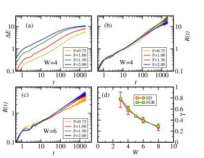
Figure 1: Results of full time propagation on systems with $L=14$ for energy increase $\Delta E(t)$ in (a), and $R(t)$ in (b) and (c). In (d) $\gamma$ vs. $W$ is shown, as obtained from fitting $R(t)\propto t^{\gamma}$ for $t\gtrsim 1$ in case of ED (circles) and using FGR (squares). In the latter case $\gamma$ was extracted from $\langle x^{2}(t)\rangle_{0}\propto t^{\gamma}$, see Ref. Prelovšek et al. (2018). Note that unless otherwise specified, we have used: $\omega_{0}=g=1$, and $t_{g}=0.5$.

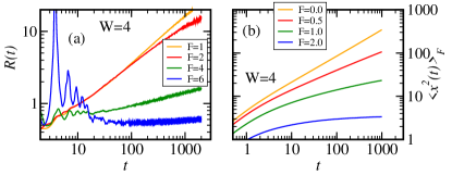
Figure 2: In (a) we show $R(t)$ for $W=4$ for different $F>0$, up to maximal $F=6$ using ED on $L=14$ sites, and in (b) the spread $\langle x^{2}(t)\rangle_{F}$, using FGR for $L=400$.

Fig. 2a shows numerical results for $R(t)$ for a fixed disorder strength $W$ but various drivings $F$. It is evident that for stronger driving $F>2$, exponent $\gamma$ (as well as particle dynamics) is significantly reduced and eventually, for very strong $F\sim 6$ the particle becomes almost localized, here due to the Stark phenomenon.

Dynamics via rate equations.– In the following we describe the system’s dynamics using the rate equations for the transitions between the localized Anderson states. The method has been shown to reproduce for $F=0$ the subdiffusive particle dynamics as well as (at least qualitatively) values for the exponent $\gamma$, Prelovšek et al. (2018). Direct comparison of numerical results obtained from ED and the rate equations is shown in the Supplemental Metarial sup . We stress that it is essential to study the distribution of the transition rates and not just their average values, since the averaging erases the essential information on their large and singular fluctuations. In particular, averaging of localized and delocalized samples would (mistakenly) indicate that the particle is always delocalized.

Here, we recall only main steps of Ref.  Prelovšek et al. (2018) for derivation of the transition rates, now taking into account $F\neq 0$. First we solve the single–particle eigenproblem for open boundary conditions

$$\sum_{j}\left[-t_{h}(c^{\dagger}_{j+1}c_{j}+{\mathrm{h}.c.})+(h_{j}-jF)n_{j}\right]=\sum_{l}\epsilon_{l}\varphi^{\dagger}_{l}\varphi_{l},$$ (4)

where $\varphi^{\dagger}_{l}=\sum_{j}\phi_{lj}c^{\dagger}_{j}$ creates a particle in the localized Anderson–Stark state $|l\rangle$. Using the FGR one obtains transition rates between states $l,l^{\prime}$ which originate from the coupling to HCB,

$$\Gamma_{l,l^{\prime}} = \int_{-\infty}^{\infty}{\mathrm{d}}t\;e^{-it\Delta_{l,l^{\prime}}}\frac{1}{L}\sum_{q}|\eta_{l,l^{\prime},q}|^{2}$$ (5)

$$\times\left[f(\omega_{q})e^{-i\omega_{q}t}+f(-\omega_{q})e^{i\omega_{q}t}\right],$$

$$\eta_{l,l^{\prime},q} = g\sum_{j}\mathrm{e}^{-iqj}\phi_{l^{\prime}j}\phi_{lj},$$ (6)

where $\omega_{q}=\omega_{0}-2t_{B}\cos(q)$, $f(\omega_{q})$ is the Fermi-Dirac distribution function and $\Delta_{l,l^{\prime}}=\epsilon_{l}-\epsilon_{l^{\prime}}$. Within the FGR, the particle dynamics can be described via the rate equations for occupations $n_{l}(t)=\langle\varphi^{\dagger}_{l}\varphi_{l}\rangle(t)$,

$$\frac{{\rm d}n_{l}}{{\rm d}t}=\sum_{l^{\prime}}(\Gamma_{l^{\prime}l}n_{l^{\prime}}-\Gamma_{ll^{\prime}}n_{l}).$$ (7)

Fig. 2b shows the evolution of the averaged spread, $\langle x^{2}(t)\rangle_{F}=\sum_{l}(x_{l}-x_{l_{0}})^{2}n_{l}(t)$, where $x_{l}=\sum_{j}j|\phi_{lj}|^{2}$, as obtained via rate equations at $\beta\to 0$ for $L=400$ and open boundary conditions. Particle is initially put in the middle of the system, well away from the boundaries, i.e., $n_{l}(0)=\delta_{l,l_{0}}$. Due to strong disorder, $W=4$, the particle spread is subdiffusive already for $F=0$. For larger $F>1$, the diffusion further slows down and eventually for $F\geq 2$ the particle tends to localize due to the Stark effect, i.e., $\langle x^{2}(t\to\infty)\rangle_{F}$ saturates. We stress a clear qualitative similarity between the spread and the rescaled drift, $R(t)$, shown in Fig. 2a. This similarity persists even when both quantities are determined for strong $F$, well beyond the the LR regime relevant for Eq. (1).

Eqs. (5)-(7) can be studied numerically even for large systems. However, in order to derive the GER within rate-equation approach, we rewrite Eq. (5) in a more symmetric form, representing it as $\Gamma_{l,l^{\prime}}=\Gamma^{0}_{l,l^{\prime}}[1+\tanh(\beta\Delta_{l,l^{\prime}}/2)]$, where $\Gamma^{0}_{l,l^{\prime}}$ refer to rates for $\beta\rightarrow 0$,

$$\Gamma^{0}_{l,l^{\prime}}=\frac{\pi}{L}\sum_{q}|\eta_{l,l^{\prime},q}|^{2}\left[\delta(\omega_{q}+\Delta_{l,l^{\prime}})+\delta(\omega_{q}-\Delta_{l,l^{\prime}})\right].$$ (8)

In general, $F\neq 0$ enters via the (symmetric) overlaps, $\eta_{l,l^{\prime},q}=\eta_{l^{\prime},l,q}$, and the (antisymmetric) energy differences, $\Delta_{l,l^{\prime}}=-\Delta_{l^{\prime},l}$. The antisymmetry of $\Gamma_{l,l^{\prime}}$ originates solely from $\tanh(\beta\Delta_{l,l^{\prime}}/2)$. The time-evolution of the particle drift due to $F\neq 0$ can be evaluated as the current, $I(t)={\rm d}\langle x(t)\rangle/{\rm dt}=\sum_{l}x_{l}{\rm d}n_{l}/{\rm dt}$. Using Eq. (7) one then obtains

$$I(t) = -\sum_{l,l^{\prime}}\frac{(x_{l}-x_{l^{\prime}})^{2}}{2}\Gamma^{0}_{l,l^{\prime}}\times$$ (9)

$$\left[\frac{n_{l}-n_{l^{\prime}}}{x_{l}-x_{l^{\prime}}}+(n_{l}+n_{l^{\prime}})\frac{\tanh[\frac{\beta(\epsilon_{l}-\epsilon_{l^{\prime}})}{2}]}{x_{l}-x_{l^{\prime}}}\right].$$

For high $T$, the second term may be expanded in $\beta$. Then, Eq.  (9) becomes the Einstein relation which states that the current is induced by the gradient of the particle density (first term) and the gradient of the potential (second term), where the latter is weighted by $\beta$ and the local density, $(n_{l}+n_{l^{\prime}})/2$.

For strong disorder and weak $F$ one may assume that $\epsilon_{l}\simeq\epsilon^{0}_{l}-x_{l}F$, where $\epsilon^{0}_{l}$ refers the Anderson state at $F=0$. Since on average $\epsilon^{0}_{l}-\epsilon^{0}_{l^{\prime}}$ vanishes, the term $(\epsilon^{0}_{l}-\epsilon^{0}_{l^{\prime}})/(x_{l}-x_{l^{\prime}})$ does not contribute to the uniform current. Then, the meaning of Eq. (9) becomes even more evident,

$$I(t) \simeq \sum_{l,l^{\prime}}\frac{(x_{l}-x_{l^{\prime}})^{2}}{2}\Gamma^{0}_{l,l^{\prime}}\left[-\frac{n_{l}-n_{l^{\prime}}}{x_{l}-x_{l^{\prime}}}+\frac{n_{l}+n_{l^{\prime}}}{2}\beta F\right].$$

We may further simplify the analysis by neglecting the explicit momentum dependence of $|\eta_{l,l^{\prime},q}|^{2}$,

$$|\eta_{l,l^{\prime},q}|^{2}\simeq|\eta_{l,l^{\prime}}|^{2}=\frac{1}{L}\sum_{q}|\eta_{l,l^{\prime},q}|^{2}=g^{2}\sum_{i}(\phi_{l^{\prime}i}\phi_{li})^{2}.$$ (11)

and assume an uniform bosonic density of states $1/L\sum_{q}\delta(\omega-\omega_{q})\simeq\frac{1}{\Omega}\theta(\Omega-\omega)$ where $\Omega=\omega_{0}+2t_{B}$. Then the transition rates at $\beta\rightarrow 0$ read

$$\Gamma^{0}_{l,l^{\prime}}\simeq\pi|\eta_{l,l^{\prime}}|^{2}\frac{1}{\Omega}\theta(\Omega-|\Delta_{l,l^{\prime}}|).$$ (12)

In order to explain the interplay between strong disorder and strong driving we calculate $\Gamma_{l}=\sum_{l^{\prime}\neq l}\Gamma^{0}_{l,l^{\prime}}$ representing the inverse lifetime of a particle occupying the Anderson state $|l\rangle$, $\tau_{l}=1/\Gamma_{l}$. As stressed before, it is essential to avoid averaging of $\Gamma_{l}$ over disorder. Instead one may consider it as a random variable and discuss the probability density $f_{\Gamma}(\Gamma_{l})$ or equivalently $f_{\tau}(\tau_{l})$. Without driving Prelovšek et al. (2018); Kozarzewski et al. (2018), the qualitative transport properties can be read out from the latter distribution using the random–trap model Bouchaud and Georges (1989). Namely, for $f_{\tau}(\tau_{l})\propto 1/\tau_{l}^{\alpha+1}$ the normal diffusive transport exists for $\alpha\geq 1$, whereas for $0<\alpha<1$ the particle spreads subdiffusively with $\langle x^{2}(t)\rangle\propto t^{\gamma}$ and $\gamma=2\alpha/(1+\alpha)$. By comparing the cumulative distribution functions one finds that the distribution $f_{\tau}(\tau_{l})\propto 1/(\tau_{l})^{\alpha+1}$ corresponds to $I(\Gamma)=\int_{0}^{\Gamma}f_{\Gamma}(\Gamma_{l}){\rm d}\Gamma_{l}\propto\Gamma^{\alpha}$, so the type of dynamics (i.e., the value of $\alpha$) can be recognized directly from $I(\Gamma)$.

Fig. 3 shows the FGR results for $I(\Gamma)$. Results in panels a) and b) are obtained from Eqs. (5)-(6), whereas panel c) shows results for the simplified transition rates, Eq. (12), labeled as Toy-model. The dashed lines show $I(\Gamma)\propto\Gamma$ hence they mark the threshold for the normal diffusive transport. Comparing panels b) and c) it becomes quite evident that simplification via Eq. (11) is very accurate. One may also see that upon increasing $F$, the exponent $\alpha$ decreases and eventually becomes vanishingly small for $F\geq 2$. The latter result means that $f_{\Gamma}(\Gamma_{l})$ acquires a $\delta(\Gamma_{l})$ contribution or, in other words, that some states remain localized despite being coupled to HCB. Since this effect originates from strong electric field, it is legitimate to attribute it as the Stark localization.

Finally, we argue that the Stark localization doesn’t occur if the particle is coupled to standard bosons, e.g., phonons. Then, the multi–boson processes significantly contribute to the transition rates, whereas previously, such contributions were strongly suppressed by the hard core–effects. As argued for the standard bosons Prelovšek et al. (2018), the rigid cut-off in Eq. (12) should be replaced by a smooth exponential cut-off, $\theta(\Omega-|\Delta_{l,l^{\prime}}|)\rightarrow\exp(-|\Delta_{l,l^{\prime}}|/\Omega)$. This seemingly harmless modification, changes the distribution of the transition rates, as shown in Fig. 3d. Even for very strong drivings and for very strong disorder the transitions rates are bounded from below $\Gamma_{l}\geq\Gamma_{\rm min}$. Therefore, the diffusion constant might be very small but nevertheless nonzero. Although the subdiffusive transport may show up for a quite long time-window, it is a transient phenomenon that will eventually be replaced by a normal diffusion, irrespectively of $W$ or $F$.

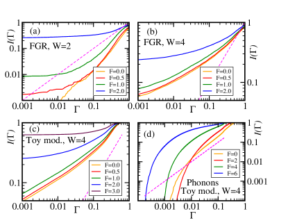
Figure 3: Cumulative distributions $I(\Gamma)$ in panels a) and b) for different $F$ were obtained from Eqs. (5)-(6), based on FGR. In panel (c) we show results for the simplified (toy model) rates as given by, Eq. (12). The dashed lines in all panels represent the threshold for normal diffusion, $I(\Gamma)\propto\Gamma$.

The GER is expected to hold true within the LR theory Steinigeweg et al. (2009); Bouchaud and Georges (1989), whereas we have demonstrated that it remains applicable (at least qualitatively) for stronger drivings when assumptions of LR are not fulfilled in an obvious way. We note that in deriving Eq. (9) from the master equation (7) we have not assumed that driving is weak or that the transport is normal diffusive, since the anomalous transport and nonlinear (in $F$) effects are encoded in $\Gamma^{0}_{l,l^{\prime}}$, see Eq. (12). The essential step in our derivation consist in expanding $\tanh[\frac{\beta(\epsilon_{l}-\epsilon_{l^{\prime}})}{2}]$ linearly in $F$. Here, $\beta$ is the temperature of the bosonic bath so the bosonic bath must be in equilibrium (or close to equilibrium) and the expansion is justified when $\beta$ is small.

One may also expect that the present model is oversimplified in that it describes only single quantum particle coupled to mutually noninteracting HCB. A more realistic description should account for nonzero density of fermions which, in turn, may induce effective interactions among the HCB. In order to check how the latter phenomena affects results presented in this manuscript, we have studied a similar system but with a boson-boson interactions. Results shown in the Supplemental Material sup demonstrate that our qualitative conclusions hold true also for mutually interacting HCB Bonča et al. (2018).

Conclusions. – We have studied the transport properties of a quantum particle that propagates along a disordered chain and is coupled to hard–core bosons, whereby such a case can be considered as the simulation of the charge motion in the spin background in strongly correlated disordered systems. Without external driving, the particle exhibits anomalous subdiffusive propagation with vanishing diffusion constant. The main goal was to establish whether a generalized Einstein relation holds true in such a system. Namely, we have studied the relation between the drift originating from the electric field ($F$) and the spread of the particle density which grows in time mainly due to its inhomogeneous spatial distribution. Both quantities were determined in the presence of $F$. The GER was shown to hold true in the LR regime (as expected) but also within the quasiequilibrium evolution, when the energy (temperature) increases in time due to driving. In particular, we have demonstrated that a single exponent $\gamma$ characterizes the anomalous dynamics of the spread $\langle x^{2}(t)\rangle_{F}$ and the drift $\langle x(t)\rangle_{F}\propto\langle x^{2}(t)\rangle_{0}\propto t^{\gamma}$. Quite unexpectedly, the latter similarity between $\langle x^{2}(t)\rangle_{F}$ and $\langle x(t)\rangle_{F}$ holds true also for much stronger fields beyond the regime of quasiequilibrium evolution. However for strong fields, $\gamma$ decreases with increasing $F$ and eventually, for very strong $F$, it vanishes marking the field-induced Stark localization. Qualitatively, all these properties were demonstrated to follow from the distribution of the transition rates between the Anderson states. We have also argued that the subdiffusive transport and localization should not occur when the particle is coupled to regular itinerant bosons with unbounded energy spectrum. In the latter case, strong driving may lead to a transient slowing down of the particle dynamics, nevertheless the asymptotic transport is expected to be normal diffusive. We cannot exclude that within a more accurate treatment of the multi-boson processes the normal diffusion eventually shows up also in the HCB model, however, for much longer times than for regular bosons.

Supplemental Material

In the Supplemental Material we discuss the finite–size (FS) effects for the exact diagonalization (ED) results. Further on, we compare numerical results obtained from ED and the rate equations (RE) where transition rates are estimated from the Fermi golden rule (FGR). Finally, we present results for a chain where the hard-core boson (HCB) mutually interact with each other.

I Details of numerical calculations and finite–size effects

Numerical ED calculations were performed using full Hilbert spaces on one-dimensional clusters with periodic boundary conditions. First, we have used standard Lanczos procedure to compute ground state wavefunction $\psi(t=0)$ for each realization of random potentials $h_{j}\in[-W,W]$. The time evolution of the initial state was then calculated by step–vise change of the Peierls phase $\delta\phi(t)=F\delta t$ in small time increments $\delta t=0.02$ at each step using Lanczos basis generating the time–evolution $\psi(t-\delta t)\to\psi(t)$. Special attention was used to check the independence of results against the choice of the time–step. The dependence of results on system sizes is presented in Fig. S1 where we show $R(t)$ using different system sizes ranging from $L=10$ to $L=15$. Curves, representing different system sizes are nearly overlapping, indicating that finite-size effects are inessential at least for qualitative conclusions. In addition, we display in Fig. S3 results for two different system sizes also for the generalized model with interacting HCB’s.

In Fig. S1c we show results obtained from FGR and RE on a set of different system sizes ranging from $L=50$ to $L=400$. Here, we average in fixed random-configuration results over all initial sites in the system (away from boundaries) and in addition over $N_{s}\sim 10$ random samples. Results thus become $L$ independent provided that $\langle x^{2}(t)\rangle\ll L^{2}$.

II Direct comparison between exact-diagonalization and the Fermi-golden-rule results

In this section we discuss numerical results which enable quantitative comparison of ED and RE [Eq. (7) in the main text] with transition rates obtained from the FRG [Eq. (5) in the main text]. Although the RE may be formally applied to a particle propagating on a finite lattice, this particle must be coupled to an infinite bosonic bath, since the FGR requires a continuous density of states. In contrast to ED, our system sizes $L\sim 400$ are free from the FS effects, as long as the spread $\langle x^{2}(t)\rangle\ll L^{2}$. In the preceding section we have shown that numerical result for ED weakly depend on $L$. Therefore, we compare numerical results for the largest system sizes, i.e. ED for $L=14$ with RE for $L=400$, see Fig. S1(c).

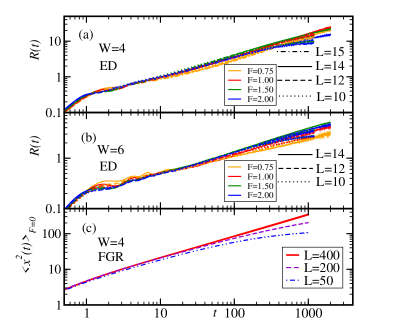
Figure S1: $R(t)$ using ED for system sizes $L=10,12,14$ in (a) and (b) and also $L=15$ in (a). Results are shown for identical parameters of the model as in Fig. 1 of the main paper: $\omega_{0}=g=1$, and $t_{g}=0.5$. In (a) there are 4 nearly overlapping curves for each value of $F$ representing results for $L=12,14,$ and 15. Similarly in (b), there are 3 nearly overlapping curves for each $F$. In (c) we present RE data based on FGR for $<x^{2}(t)>_{F=0}$ for different system sizes ranging from $L=50$ through 400.

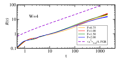
Figure S2: The same as Fig. S1a but compared with $\frac{1}{4}\langle x^{2}(t)\rangle_{F=0}$ (violet dashed line) as obtained from RE based on FGR without driving, $F=0$.

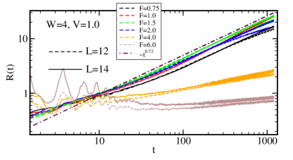
Figure S3: $R(t)$ for $W=4$ and $V=1$ for different $F>0$, up to maximal $F=6$ using ED on $L=12$ (dashed lines) and 14 sites (full lines). Dot-dashed line represents $R(t)\propto t^{0.72}$. Other parameters of the model are the same as in Fig. S1.

Within the high-temperature expansion one obtains the kinetic energy of a single particle, $E_{k}=-2\beta$. Introducing this relation into Eqs. (1) and (3) in the main text one obtains the Einstein relation $R(t)=\frac{1}{4}\langle x^{2}(t)\rangle$, where $R(t)=-\Delta E(t)/F^{2}E_{k}(t)$. Figure S2 shows $R(t)$ obtained from ED in comparison with the spread $\frac{1}{4}\langle x^{2}(t)\rangle_{F=0}$ obtained from RE together with FGR. The quantitative comparison might seem dissatisfactory, since the results clearly differ. However, we notice that differences between both methods arise during the short time dynamics, $t\lessapprox 5$, whereas for longer times both methods give consistent results since curves remain parallel to each other. It is rather clear that the latter differences cannot originate from the FS effects, since FS should be most visible at longer times when the spread of particle becomes comparable to the system size. The differences between both methods may partially originate from different initial states: in the RE we start from a chosen Anderson state while in ED from the ground state of $H$, Eq. 1 (in the main text), before the onset of driving. Nevertheless, the origin of these difference should be attributed predominantly to the failure of the RE for short–times. Since RE represent the classical master equation it must fail if the propagation time is smaller than the decoherence time. To conclude this section, we notice that the RE and ED results obtained for the largest accessible system sizes are consistent except for the short time-window, where the failure of the RE is well justified and expected.

III Interacting Hard–Core Bosons

As argued in the main text, in the case of nonvanishing density of fermions, the fermion-boson interaction may induce an effective interactions among the HCB. Following this arguments, in this section we present additional test for the robustness of the GER by introducing interaction $V$ between HCB’s located on neighboring sites. The introduction of small $V$ lifts the degeneracy among itinerant HCB states. Further increase of $V$ leads to slowing down the propagation of excitations while it concurrently increases the energy of excitations in the HCB subspace. Generalization of the original model to interacting HCB’s thus represents a suitable model to test the stability of GER.

In Fig. S3 we present results for $R(t)$ obtained for a generalized interacting HCB model:

$$H_{U} = -t_{h}\sum_{j}(c^{\dagger}_{j+1}c_{j}+{\mathrm{h}.c.})+\sum_{j}h_{j}n_{j}+g\sum_{j}n_{j}(a^{\dagger}_{j}+a_{j})$$ (S1)

$$+ \omega_{0}\sum_{j}a_{j}^{\dagger}a_{j}-t_{b}\sum_{j}(a_{j+1}^{\dagger}a_{j}+\mathrm{H.c.})$$

$$+ V\sum_{j}a_{j}^{\dagger}a_{j}a_{j+1}^{\dagger}a_{j+1}.$$

Apart for larger extracted $\gamma=0.72$, in comparison to $\gamma=0.58$ in the case of itinerant HCB’s, results are very similar to the ones, presented in Fig. 2(a) of the main text. For small driving up to $F\lesssim 2.0$ we observe scaling, characteristic for GER. The increase of $\gamma$ in comparison to itinerant HCB’s may be attributed to a combination of lifting of the degeneracy as well as to the increased energy of HCB excitations that in turn increases the ability of the HCB subspace to absorb energy from the driving. For stronger driving $F>2$, exponent $\gamma$ (as well as particle dynamics) is significantly reduced and eventually, for very strong $F\sim 6$ the particle becomes almost localized.