Predict-and-recompute conjugate gradient variants

Abstract

The standard implementation of the conjugate gradient algorithm suffers from communication bottlenecks on parallel architectures, due primarily to the two global reductions required every iteration. In this paper, we study conjugate gradient variants which decrease the runtime per iteration by overlapping global synchronizations, and in the case of pipelined variants, matrix-vector products. Through the use of a predict-and-recompute scheme, whereby recursively-updated quantities are first used as a predictor for their true values and then recomputed exactly at a later point in the iteration, these variants are observed to have convergence behavior nearly as good as the standard conjugate gradient implementation on a variety of test problems. We provide a rounding error analysis which provides insight into this observation. It is also verified experimentally that the variants studied do indeed reduce the runtime per iteration in practice and that they scale similarly to previously-studied communication-hiding variants. Finally, because these variants achieve good convergence without the use of any additional input parameters, they have the potential to be used in place of the standard conjugate gradient implementation in a range of applications.

65F10, 65N12, 65Y05

1 Introduction and background

The conjugate gradient method (CG), due to Hestenes and Stiefel [22], is a widely-used method for solving a linear system of equations $\mathbf{A}\mathbf{x}=\mathbf{b}$, when $\mathbf{A}\in\mathbb{R}^{n\times n}$ is a large symmetric positive definite matrix. While the low storage costs and low number of floating point operations per iteration make CG an attractive choice for solving very large sparse systems, the dependency structure of the standard conjugate gradient algorithm given in [22], which we call HS-CG and present in Algorithm 1, requires that nearly every computation be done in sequence. In particular, it requires two inner products and one (typically sparse) matrix-vector product per iteration, none of which can occur simultaneously. On distributed memory parallel systems, this results in a communication bottleneck [13, 1, 2, 14]. This is because inner products require a costly global reduction involving communication between all nodes, and the matrix-vector product, even if sparse or structured, requires some level of communication between individual nodes.

To address this bottleneck, many mathematically equivalent variants of the CG method have been introduced; see for instance [30, 31, 5, 25, 32, 6, 36, 16, 15, 9, 10, etc.]. Broadly speaking, these variants rearrange the HS-CG algorithm such that the communication occurs less frequently or is overlapped with other computations. As a result, the time per iteration of these methods may be reduced on parallel machines in certain settings. The algorithmic variants of CG presented in this paper are most closely related to the communication-hiding variants which we call M-CG, CG-CG, and GV-CG (pipelined CG), introduced by Meurant [25], Chronopoulos and Gear [6], and Ghysels and Vanroose [16], respectively. These communication-hiding variants maintain the iteration structure of HS-CG but add auxiliary vectors such that the computations within an iteration can be arranged so that expensive ones can occur simultaneously, effectively “hiding” the cost of communication. A comparison of these variants is given in Table 1 and full descriptions are given in Appendix D.

Algorithm 1 Hestenes and Stiefel Conjugate Gradient (preconditioned)

1:procedure HS-CG($\mathbf{A}$, $\mathbf{M}$, $\mathbf{b}$, $\mathbf{x}_{0}$)

2:     initialize()

3:     for $k=1,2,\ldots$ do

4:         $\mathbf{x}_{k}=\mathbf{x}_{k-1}+\alpha_{k-1}\mathbf{p}_{k-1}$

5:         $\mathbf{r}_{k}=\mathbf{r}_{k-1}-\alpha_{k-1}\mathbf{s}_{k-1}$,  $\tilde{\mathbf{r}}_{k}=\mathbf{M}^{-1}\mathbf{r}_{k}$

6:         $\nu_{k}=\langle\tilde{\mathbf{r}}_{k},\mathbf{r}_{k}\rangle$

7:         $\beta_{k}=\nu_{k}/\nu_{k-1}$

8:         $\mathbf{p}_{k}=\tilde{\mathbf{r}}_{k}+\beta_{k}\mathbf{p}_{k-1}$

9:         $\mathbf{s}_{k}=\mathbf{A}\mathbf{p}_{k}$

10:         $\mu_{k}=\langle\mathbf{p}_{k},\mathbf{s}_{k}\rangle$

11:         $\alpha_{k}=\nu_{k}/\mu_{k}$

12:     end for

13:end procedure

Notably, however, many communication-hiding variants suffer from numerical problems due to this rearranging of computations within each iteration. Indeed, it is well known that CG is particularly sensitive to rounding errors and any modification to the HS-CG algorithm can have a significant effect on numerical behavior; see [19, 27] for summaries of CG and Lanczos in finite precision. Specifically, both the rate of convergence (the number of iterations to reach a given level of accuracy) and the maximal attainable accuracy of any algorithmic variant of CG may be severely impacted by carrying out computations in finite precision.

These effects are particularly pronounced in pipelined methods, such as GV-CG, because the additional auxiliary recurrences can cause rounding errors to be amplified [4]. For example, as shown in Section 4, there are many problems for which the final accuracy attainable by GV-CG is orders of magnitude worse than that attainable by HS-CG. As a result, the practical use of some of the pipelined variants is potentially limited because the algorithms may fail to reach an acceptable level of accuracy, or require so many iterations to do so that there is no benefit to the overall runtime. While there have been many approaches to improving the numerical properties of these variants, such as residual replacement [16, 8] and the use of shifts in auxiliary recurrences [9], these strategies typically require certain parameters to be selected ahead of time based on user intuition or rely on heuristics for when and how to apply corrections. Moreover, as in the case of residual replacement, these strategies sometimes result in delayed convergence.

In this paper, we present a communication-hiding variant similar to M-CG which requires a single global synchronization per iteration. Like the M-CG algorithm, our variants employ a predict-and-recompute scheme which recursively computes quantities as a predictor for their true values and then recomputes them later in the iteration. We then introduce “pipelined” versions of both this variant and of M-CG which allow the computation and communication from the matrix-vector product and preconditioning steps to be overlapped with the global reduction associated with the inner products. We demonstrate numerically that the convergence behavior of our pipelined variants is comparable to that of HS-CG despite overlapping all matrix products with global reductions as in other pipelined variants such as GV-CG. This observation is complemented by a rounding error analysis, which provides new insight into the way the predict-and-recompute schemes can improve the numerical behavior. More broadly, this work demonstrates that it is reasonable to add extra computation to improve the numerical properties of a communication-hiding CG variant, provided that that the computation is done in a way which does not affect the communication pattern of the algorithm. All of the algorithms introduced in this paper require exactly the same inputs as HS-CG and therefore require no additional tuning by the end user.

Our primary contributions are as follows. First, we provide rounding error analyses of the variants introduced in this paper. In particular, we derive expressions for the residual gap, which is the quantity that dictates the maximum attainable accuracy, as well as for the error in the three-term Lanczos recurrence, which gives some inidcation of the rate of convergence. Our analysis provides a rigorous explanation to a conjecture made by Meurant in [25] that the predict-and-recompute scheme resolves a potential source of instability. In addition, we provide a range of numerical experiments to further support the claim that our pipelined variants can significantly improve the rate of convergence and ultimately attainable accuracy versus existing pipelined variants. In particular, we note that in the numerical experiments in Section 4, our variants appear to converge similarly HS-CG without any additional input parameters. As such, they have the potential to be used as black box solvers wherever HS-CG is used. Finally, we demonstrate through a strong scaling experiment that the new variants can reduce the time per iteration in a parallel setting.

Unless otherwise stated, matrices should be assumed to be of size $n\times n$ and vectors of size $n\times 1$. The transpose of a matrix is denoted with the superscript T, and the inverse of the transpose denoted with the superscript $-\textsf{T}$. The standard Euclidean inner product and corresponding spectral/operator norm are respectively denoted $\langle\cdot,\cdot\rangle$ and $\|\cdot\|$, and the inner product and norm induced by a positive definite matrix $\mathbf{B}$ are denoted $\langle\cdot,\cdot\rangle_{\mathbf{B}}$ and $\|\cdot\|_{\mathbf{B}}$. While much of the theory about the conjugate gradient algorithm applies to complex systems, we consider real systems for convenience.

The variants studied in this paper are all compatible with a preconditioner $\mathbf{M}^{-1}=\mathbf{R}^{-\textsf{T}}\mathbf{R}^{-1}$, which allows the algorithms to implicitly solve the system $\mathbf{R}^{-\textsf{T}}\mathbf{A}\mathbf{R}^{-1}\mathbf{y}=\mathbf{R}^{-\textsf{T}}\mathbf{b}$ and then set $\mathbf{x}=\mathbf{R}^{-1}\mathbf{y}$, using only products with $\mathbf{M}^{-1}$; i.e. the $\mathbf{R}^{-1}$ factors need not be known. As summarized in Table 1, the preconditioned variants require some additional memory to store the preconditioned residual and any related auxiliary vectors, and updating these additional vectors has the potential to introduce additional rounding errors. Throughout this paper, we use a tilde (“ $\sim$ ”) above a vector to indicate that, in exact arithmetic, the tilde vector is equal to the preconditioner applied to the non-tilde vector; i.e., $\tilde{\mathbf{r}}_{k}=\mathbf{M}^{-1}\mathbf{r}_{k}$, $\tilde{\mathbf{s}}_{k}=\mathbf{M}^{-1}\mathbf{s}_{k}$, etc.

variant	mem.	vec.	scal.	time
HS-CG	4 (+1)	3 (+0)	2	$2\,\mathrm{C}_{\text{gr}}+\mathrm{T}_{\text{mv}}+\mathrm{C}_{\text{mv}}$
CG-CG	5 (+1)	4 (+0)	2	$\mathrm{C}_{\text{gr}}+\mathrm{T}_{\text{mv}}+\mathrm{C}_{\text{mv}}$
M-CG	4 (+2)	3 (+1)	3	$\mathrm{C}_{\text{gr}}+\mathrm{T}_{\text{mv}}+\mathrm{C}_{\text{mv}}$
PR-CG	4 (+2)	3 (+1)	4	$\mathrm{C}_{\text{gr}}+\mathrm{T}_{\text{mv}}+\mathrm{C}_{\text{mv}}$
GV-CG	7 (+3)	6 (+2)	2	$\max(\mathrm{C}_{\text{gr}},\mathrm{T}_{\text{mv}}+\mathrm{C}_{\text{mv}})$
pipe-M-CG	6 (+4)	5 (+3)	3	$\max(\mathrm{C}_{\text{gr}},\mathrm{T}_{2\text{mv}}+\mathrm{C}_{\text{mv}})$
pipe-PR-CG	6 (+4)	5 (+3)	4	$\max(\mathrm{C}_{\text{gr}},\mathrm{T}_{2\text{mv}}+\mathrm{C}_{\text{mv}})$

Table 1: Summary of costs for various conjugate gradient variants. Values in parenthesis are the additional costs for the preconditioned variants. The quantity mem. gives the number of vectors stored, vec. gives the number of vector updates (AXPYs) per iteration, scal. gives the number of inner products per iteration, and time gives the dominant costs (ignoring vector updates and inner products). $\mathrm{C}_{\text{gr}}$ is the time spent on communication for a global reduction. $\mathrm{T}_{\text{mv}}$ and $\mathrm{C}_{\text{mv}}$ are the times spent on computation and communication, respectively, for a matrix-vector product which depend on the method of matrix multiplication (for instance a dense matrix has $\mathrm{C}_{\text{mv}}=\mathrm{C}_{\text{gr}}$). $\mathrm{T}_{2\text{mv}}$ is the cost of computing two matrix vector products simultaneously, which is less than $2\,\mathrm{T}_{\text{mv}}$ if implemented in an efficient way. Note that in this abstraction we assume that the communication time is independent of the size of messages sent.

2 Derivation of new variants

In this section we describe PR-CG, a new communication-hiding variant which requires only one global synchronization point per iteration. This variant is similar to M-CG, introduced by Meurant in [25], and the relationship between the two algorithms is discussed.

Then, in the same way that GV-CG is obtained from CG-CG, we “pipeline” PR-CG to overlap the matrix-vector product with the inner products. The order in which operations are done in the pipelined version of PR-CG allows for a vector quantity to be recomputed using an additional matrix-vector product, giving the pipelined predict-and-recompute variant pipe-PR-CG. Since this matrix-vector product can occur at the same time as the other matrix-vector product and as the inner products, the communication costs per iteration are not increased. For comparison, we also derive a pipelined version of Meurant’s M-CG method, which we call pipe-M-CG.

Table 1 provides a comparison between some commonly used communication avoiding variants and the newly introduced variants. It should be noted that although the number of matrix-vector products and inner products in pipe-M-CG and pipe-PR-CG are increased, most of this work can be done locally, and they have the same dominant communication costs as GV-CG.

2.1 A simple communication-hiding variant

Like the derivation of M-CG in [25] and the variants introduced in [23, 30, 31, 32], we derive PR-CG by substituting recurrences into the inner product $\nu_{k}=\langle\tilde{\mathbf{r}}_{k},\mathbf{r}_{k}\rangle$. This allows us to obtain an equivalent expression for the inner product involving quantities which are known earlier in the iteration.

To this end, we first recall that given $\tilde{\mathbf{s}}_{k}=\mathbf{M}^{-1}\mathbf{s}_{k}$, we have

(1) $$\tilde{\mathbf{r}}_{k}=\tilde{\mathbf{r}}_{k-1}-\alpha_{k-1}\tilde{\mathbf{s}}_{k-1}.$$

Then, by substituting the recurrences for $\tilde{\mathbf{r}}_{k}$ and $\mathbf{r}_{k}$ from Algorithm 1 into $\nu_{k}=\langle\tilde{\mathbf{r}}_{k},\mathbf{r}_{k}\rangle$, we can write

$$\nu_{k} =\langle\tilde{\mathbf{r}}_{k-1}-\alpha_{k-1}\tilde{\mathbf{s}}_{k-1},\mathbf{r}_{k-1}-\alpha_{k-1}\mathbf{s}_{k-1}\rangle$$

(2) $$=\langle\tilde{\mathbf{r}}_{k-1},\mathbf{r}_{k-1}\rangle-\alpha_{k-1}\langle\tilde{\mathbf{r}}_{k-1},\mathbf{s}_{k-1}\rangle-\alpha_{k-1}\langle\tilde{\mathbf{s}}_{k-1},\mathbf{r}_{k-1}\rangle+\alpha_{k-1}^{2}\langle\tilde{\mathbf{s}}_{k-1},\mathbf{s}_{k-1}\rangle.$$

Since $\mathbf{M}$, and therefore $\mathbf{M}^{-1}$, are symmetric, $\langle\tilde{\mathbf{s}}_{k-1},\mathbf{r}_{k-1}\rangle=\langle\mathbf{s}_{k-1},\tilde{\mathbf{r}}_{k-1}\rangle$. Thus,

(3) $$\nu_{k}=\nu_{k-1}-2\alpha_{k-1}\langle\tilde{\mathbf{r}}_{k-1},\mathbf{s}_{k-1}\rangle+\alpha_{k-1}^{2}\langle\tilde{\mathbf{s}}_{k-1},\mathbf{s}_{k-1}\rangle.$$

Once $\mathbf{s}_{k}=\mathbf{A}\mathbf{p}_{k}$ and $\tilde{\mathbf{s}}_{k}=\mathbf{M}^{-1}\mathbf{s}_{k}$ have been computed, we can simultaneously compute the three inner products,

(4) $$\mu_{k}=\langle\mathbf{p}_{k},\mathbf{s}_{k}\rangle, \sigma_{k}=\langle\tilde{\mathbf{r}}_{k},\mathbf{s}_{k}\rangle, \gamma_{k}=\langle\tilde{\mathbf{s}}_{k},\mathbf{s}_{k}\rangle.$$

A variant using a similar expression for $\nu_{k}$ was suggested in [24] and briefly mentioned in [4]. However, one term of their formula for $\nu_{k}$ has a sign difference from Eq. 3, and no numerical tests or rounding error analysis were provided.

Algorithm 2 Predict-and-recompute conjugate gradient

1:procedure PR-CG($\mathbf{A}$, $\mathbf{M}$, $\mathbf{b}$, $\mathbf{x}_{0}$)

2:     initialize()

3:     for $k=1,2,\ldots$ do

4:         $\mathbf{x}_{k}=\mathbf{x}_{k-1}+\alpha_{k-1}\mathbf{p}_{k-1}$

5:         $\mathbf{r}_{k}=\mathbf{r}_{k-1}-\alpha_{k-1}\mathbf{s}_{k-1}$,  $\tilde{\mathbf{r}}_{k}=\tilde{\mathbf{r}}_{k-1}-\alpha_{k-1}\tilde{\mathbf{s}}_{k-1}$

6:         $\nu^{\prime}_{k}=\nu_{k-1}-2\alpha_{k-1}\sigma_{k-1}+\alpha_{k-1}^{2}\gamma_{k-1}$

7:         $\beta_{k}=\nu^{\prime}_{k}/\nu_{k-1}$

8:         $\mathbf{p}_{k}=\tilde{\mathbf{r}}_{k}+\beta_{k}\mathbf{p}_{k-1}$

9:         $\mathbf{s}_{k}=\mathbf{A}\mathbf{p}_{k}$,  $\tilde{\mathbf{s}}_{k}=\mathbf{M}^{-1}\mathbf{s}_{k}$

10:         $\mu_{k}=\langle\mathbf{p}_{k},\mathbf{s}_{k}\rangle$,  $\sigma_{k}=\langle\tilde{\mathbf{r}}_{k},\mathbf{s}_{k}\rangle$,  $\gamma_{k}=\langle\tilde{\mathbf{s}}_{k},\mathbf{s}_{k}\rangle$,  $\nu_{k}=\langle\tilde{\mathbf{r}}_{k},\mathbf{r}_{k}\rangle$

11:         $\alpha_{k}=\nu_{k}/\mu_{k}$

12:     end for

13:end procedure

As shown in Fig. 1, if Eq. 3 is used to recursively update $\nu_{k}$, the final accuracy can be severely impacted. This phenomenon was observed previously in [30, 23, 31], all of which study variants which use expressions for $\nu_{k}$ similar to that in M-CG. This catastrophic loss of accuracy is caused by the updated value of $\nu_{k}$ becoming negative. In [25], Meurant suggests using the recursively-updated value of $\nu_{k}$ as a predictor for the true value in order to update any vectors required for the algorithm to proceed, and then to recompute $\nu_{k}=\langle\tilde{\mathbf{r}}_{k},\mathbf{r}_{k}\rangle$ at the same time as the other inner products. We observe experimentally that using this strategy effectively brings the ultimately attainable accuracy to a level similar to that of HS-CG. Our rounding error analysis in Section 3 explains this improvement. This algorithm, denoted PR-CG, is given in Algorithm 2. Note that we use a prime (“ ^′ ”) to distinguish the recursively updated quantity $\nu^{\prime}_{k}$ from the explicitly computed quantity $\nu_{k}$.

It is not hard to see that Eq. 3 can be simplified further. Indeed, observing that $\langle\tilde{\mathbf{s}}_{k},\mathbf{r}_{k}\rangle=\langle\mathbf{p}_{k},\mathbf{s}_{k}\rangle$, which follows from the $\mathbf{A}$-orthogonality of $\mathbf{p}_{k}$ and $\mathbf{p}_{k-1}$, and using the expression $\alpha_{k}=\nu_{k}/\mu_{k}=\langle\tilde{\mathbf{r}}_{k},\mathbf{r}_{k}\rangle/\langle\mathbf{p}_{k},\mathbf{s}_{k}\rangle$, we can write

$$\nu_{k}=-\langle\tilde{\mathbf{r}}_{k-1},\mathbf{r}_{k-1}\rangle+\alpha_{k}^{2}\langle\tilde{\mathbf{s}}_{k-1},\mathbf{s}_{k-1}\rangle=-\nu_{k-1}+\alpha_{k}^{2}\langle\tilde{\mathbf{s}}_{k-1},\mathbf{s}_{k-1}\rangle.$$

This is exactly the expressions studied in [25] and used by M-CG; i.e., M-CG can be obtained by replacing line 6 of PR-CG with $\nu_{k}^{\prime}=-\nu_{k}+\alpha_{k}^{2}\gamma_{k}$. A similar expression, $\nu_{k}=-\alpha_{k}\mu_{k}+\alpha_{k}^{2}\gamma_{k}$, was studied in [36].

The natural question is then: What is the advantage of the expression for $\nu_{k}$ used in PR-CG over the expression used in M-CG? The incomplete response is that experimentally it seems to work a bit better, especially in the pipelined versions of these variants. Intuitively, this is because the less simplification that occurs, the closer the variant is to HS-CG. Of course then it is reasonable to wonder if we should use Eq. 3 instead of Eq. 2. The again incomplete response is that this change doesn’t seem to significantly influence the numerical behavior. This is perhaps not particularly surprising; for instance, in the case of the unpreconditioned variants, Eq. 2 and Eq. 3 are equivalent even in finite precision. An extended discussion on this topic is included in Appendix C; a full theoretical explanation remains future work.

2.2 New pipelined variants

Recall that our goal is to be able to compute the matrix-vector product and inner products simultaneously. To this end, note that in both M-CG and PR-CG we have the recurrence $\mathbf{p}_{k}=\tilde{\mathbf{r}}_{k}+\beta_{k}\mathbf{p}_{k-1}$. Thus, defining $\mathbf{w}_{k}=\mathbf{A}\tilde{\mathbf{r}}_{k}$, we can write

(5) $$\mathbf{s}_{k}=\mathbf{A}\mathbf{p}_{k}=\mathbf{A}\tilde{\mathbf{r}}_{k}+\beta_{k}\mathbf{A}\mathbf{p}_{k-1}=\mathbf{w}_{k}+\beta_{k}\mathbf{s}_{k-1}.$$

Similarly, defining $\mathbf{u}_{k}=\mathbf{A}\tilde{\mathbf{s}}_{k}$,

(6) $$\mathbf{w}_{k}=\mathbf{A}\tilde{\mathbf{r}}_{k} =\mathbf{A}\tilde{\mathbf{r}}_{k-1}-\alpha_{k-1}\mathbf{A}\tilde{\mathbf{s}}_{k-1}=\mathbf{w}_{k-1}-\alpha_{k-1}\mathbf{u}_{k-1}.$$

Using these recurrences allows us to compute the product $\mathbf{u}_{k}=\mathbf{A}\tilde{\mathbf{s}}_{k}$ at the same time as all of the inner products.

To move the preconditioning step, we define $\tilde{\mathbf{w}}_{k}=\mathbf{M}^{-1}\mathbf{w}_{k}$ so that

(7) $$\tilde{\mathbf{s}}_{k}=\mathbf{M}^{-1}\mathbf{s}_{k} =\mathbf{M}^{-1}\mathbf{w}_{k}+\beta_{k}\mathbf{M}^{-1}\mathbf{s}_{k-1}=\tilde{\mathbf{w}}_{k}+\beta_{k}\tilde{\mathbf{s}}_{k-1},$$

and define $\tilde{\mathbf{u}}_{k}=\mathbf{M}^{-1}\mathbf{u}_{k}$ so that

(8) $$\tilde{\mathbf{w}}_{k}=\mathbf{M}^{-1}\mathbf{w}_{k} =\mathbf{M}^{-1}\mathbf{w}_{k-1}-\alpha_{k-1}\mathbf{M}^{-1}\mathbf{u}_{k-1}=\tilde{\mathbf{w}}_{k-1}-\alpha_{k-1}\tilde{\mathbf{u}}_{k-1}.$$

The recurrences above could be used to implement a pipelined variant which, in each iteration, overlaps the matrix product and preconditioning steps with the global reduction. However, like GV-CG, this variant suffers from delayed convergence and reduced final accuracy compared to HS-CG, M-CG, and PR-CG. To address this, we observe that $\mathbf{w}_{k}=\mathbf{A}\tilde{\mathbf{r}}_{k}$ and $\tilde{\mathbf{w}}_{k}=\mathbf{M}^{-1}\mathbf{w}_{k}$ can be recomputed at the same time as the other matrix-vector product and all inner products are being computed. Thus, in the same way we use the recursively-updated value of $\nu_{k}$ as a predictor for the true value, we can use the recursively-updated value of $\mathbf{w}_{k}$ as a predictor for the true value in order to update other vector quantities, and then update the value of $\mathbf{w}_{k}$ later in the iteration. Using this predict-and-recompute approach gives pipe-M-CG and pipe-PR-CG.

Algorithm 3 Pipelined predict-and-recompute conjugate gradient

1:procedure pipe-PR-CG($\mathbf{A}$, $\mathbf{M}$, $\mathbf{b}$, $\mathbf{x}_{0}$)

2:     initialize()

3:     for $k=1,2,\ldots$ do

4:         $\mathbf{x}_{k}=\mathbf{x}_{k-1}+\alpha_{k-1}\mathbf{p}_{k-1}$

5:         $\mathbf{r}_{k}=\mathbf{r}_{k-1}-\alpha_{k-1}\mathbf{s}_{k-1}$ ,  $\tilde{\mathbf{r}}_{k}=\tilde{\mathbf{r}}_{k-1}-\alpha_{k-1}\tilde{\mathbf{s}}_{k-1}$

6:         $\mathbf{w}^{\prime}_{k}=\mathbf{w}_{k-1}-\alpha_{k-1}\mathbf{u}_{k-1}$,  $\tilde{\mathbf{w}}^{\prime}_{k}=\tilde{\mathbf{w}}_{k-1}-\alpha_{k-1}\tilde{\mathbf{u}}_{k-1}$

7:         $\nu^{\prime}_{k}=\nu_{k-1}-2\alpha_{k-1}\sigma_{k-1}+\alpha_{k-1}^{2}\gamma_{k-1}$

8:         $\beta_{k}=\nu^{\prime}_{k}/\nu_{k-1}$

9:         $\mathbf{p}_{k}=\tilde{\mathbf{r}}_{k}+\beta_{k}\mathbf{p}_{k-1}$

10:         $\mathbf{s}_{k}=\mathbf{w}^{\prime}_{k}+\beta_{k}\mathbf{s}_{k-1}$,  $\tilde{\mathbf{s}}_{k}=\tilde{\mathbf{w}}^{\prime}_{k}+\beta_{k}\tilde{\mathbf{s}}_{k-1}$

11:         $\mathbf{u}_{k}=\mathbf{A}\tilde{\mathbf{s}}_{k}$,  $\tilde{\mathbf{u}}_{k}=\mathbf{M}^{-1}\mathbf{u}_{k}$

12:         $\mathbf{w}_{k}=\mathbf{A}\tilde{\mathbf{r}}_{k}$,  $\tilde{\mathbf{w}}_{k}=\mathbf{M}^{-1}\mathbf{w}_{k}$

13:         $\mu_{k}=\langle\mathbf{p}_{k},\mathbf{s}_{k}\rangle$,  $\sigma_{k}=\langle\tilde{\mathbf{r}}_{k},\mathbf{s}_{k}\rangle$,  $\gamma_{k}=\langle\tilde{\mathbf{s}}_{k},\mathbf{s}_{k}\rangle$,  $\nu_{k}=\langle\tilde{\mathbf{r}}_{k},\mathbf{r}_{k}\rangle$

14:         $\alpha_{k}=\nu_{k}/\mu_{k}$

15:     end for

16:end procedure

Algorithm 3 shows pipe-PR-CG, from which pipe-M-CG can be obtained by using the alternate expression $\nu^{\prime}_{k}=-\nu_{k-1}+\alpha_{k-1}^{2}\gamma_{k-1}$ in line 7. Using this expression means that $\sigma_{k}$ need not be computed. As before, we use a prime to denote predicted quantities.

2.2.1 Implementation

The presentation of pipe-PR-CG in Algorithm 3 is intended to match the derivation from HS-CG and to emphasize the mathematical equivalence of the two algorithms. However, as with any parallel algorithm, some care must be taken at implementation time as an inefficient implementation may actually increase the runtime per iteration.

We suggest computing the scalars $\alpha_{k-1},\nu_{k}^{\prime},$ and $\beta_{k}$ (lines 14, 7, 8) at the beginning of each iteration. This will allow all vector updates (lines 4, 5, 6, 9, 10) to occur simultaneously. The vector updates require only local on-node communication and are therefore assumed to be very fast. Finally, the matrix-vector products/preconditioning (lines 11, 12) and inner products (line 13) can all be computed simultaneously. As a result, the dominant cost per iteration will be either the time for the global reduction associated with the inner products or with the matrix-vector products, thus giving the runtime $\max(\mathrm{C}_{\text{gr}},\mathrm{T}_{2\text{mv}}+\mathrm{C}_{\text{mv}})$ as listed in Table 1.

The matrix-vector products (and preconditioning) in lines 11 and 12 can be computed together using efficient kernels. In particular, this means that within a single node, pipe-PR-CG still requires only one pass over $\mathbf{A}$ (and $\mathbf{M}^{-1}$) in each iteration. This is an especially important consideration if $\mathbf{A}$ is too large to store in fast memory. Similarly, three of the inner products involve $\mathbf{s}_{k}$, so the number of passes over $\mathbf{s}_{k}$ can be reduced from three to one. However, this is likely not to have a noticeable effect until the cost of reading $\mathbf{s}_{k}$ from memory becomes large compared to the reduction time. Finally, there is no need to store $\mathbf{w}_{k}$ and $\mathbf{w}_{k}^{\prime}$ as separate vectors.

3 Rounding error analysis

We give a rounding error analysis which provides some insight into how predict-and-recompute schemes may lead to the improved maximal accuracy and convergence behavior observed on test problems.

The maximal attainable accuracy of a CG algorithm in finite precision is typically analyzed in terms of the residual gap $\Delta_{\mathbf{r}_{k}}:=(\mathbf{b}-\mathbf{A}\mathbf{x}_{k})-\mathbf{r}_{k}$ [18, 33], an expression introduced by Greenbaum in [17, Theorem 2]. For many variants, such as HS-CG and those introduced in this paper, it is observed experimentally that the norm of the updated residual $\mathbf{r}_{k}$ decreases to much lower than the machine precision. As a result, the size of the residual gap $\Delta_{\mathbf{r}_{k}}$ can be used to estimate of the size of the smallest true residual which can be attained in finite precision, thereby giving an estimate of the accuracy of the iterate $\mathbf{x}_{k}$. Similar analyses have been done for a three-term CG variant [21], as well as for CG-CG, GV-CG, and other pipelined CG variants [8, 4]. However, for some variants such as GV-CG, the updated residual $\mathbf{r}_{k}$ may not decrease to well below machine precision, so some care must be taken when interpreting such results.

There is also existing theory about the rate of convergence of a CG implementation in finite precision due to Greenbaum [17], which extends the work of Paige [28, 29]. This analysis applies to a perturbed Lanczos recurrence, which, in effect, shows that the error norms of a CG algorithm run in finite precision for $k$ steps correspond to the error norms of exact arithmetic CG applied to a larger matrix whose eigenvalues lie in small intervals about the eigenvalues of $\mathbf{A}$, provided that the updated residuals $\mathbf{r}_{k}$ satisfy certain conditions. This provides a method for applying the well-understood theory about the convergence of CG in exact arithmetic to the finite precision setting.

The conditions required for the analysis in [17] are that (i) successive updated residuals are approximately orthogonal; i.e., $\langle\mathbf{r}_{k},\mathbf{r}_{k-1}\rangle\approx 0$, and (ii) that they approximately satisfy the three-term Lanzos recurrence; i.e.,

(9) $$\mathbf{A}\mathbf{q}_{k} \approx\frac{1}{\alpha_{k-1}}\frac{\|\mathbf{r}_{k}\|}{\|\mathbf{r}_{k-1}\|}\mathbf{q}_{k+1}+\left(\frac{1}{\alpha_{k-1}}+\frac{\beta_{k-1}}{\alpha_{k-2}}\right)\mathbf{q}_{k}+\frac{1}{\alpha_{k-2}}\frac{\|\mathbf{r}_{k-1}\|}{\|\mathbf{r}_{k-2}\|}\mathbf{q}_{k-1},$$

where $\alpha_{k}$ and $\beta_{k}$ are computed in finite precision and $\mathbf{q}_{k+1}:=(-1)^{k}\mathbf{r}_{k}/\|\mathbf{r}_{k}\|$ is obtained from the updated residuals.

If these conditions are satisfied, then for some small $\eta$ which depends on the machine precision and on the technical definition of “approximately” (see [17] for details), the error norms will satisfy the relaxed minimax bound

(10) $$\frac{\|\mathbf{e}_{k}\|_{\mathbf{A}}}{\|\mathbf{e}_{0}\|_{\mathbf{A}}}\leq\min_{p\in\mathcal{P}_{k}}\left[\max_{z\in\mathcal{L}(\mathbf{A})}|p(z)|\right], \mathcal{L}(\mathbf{A})=\bigcup_{i=1}^{n}[\lambda_{i}-\eta,\lambda_{i}+\eta].$$

The degree to which these conditions are satisfied in finite precision directly impacts the size of $\eta$, with better approximations yielding smaller $\eta$ and therefore stronger bounds. In fact, if the conditions are exactly satisfied, then the analysis will yield $\eta=0$ and Eq. 10 becomes the well-known minimax bound for exact arithmetic CG.

However, it remains to be proved that any of the variants discussed in this paper satisfy both of the conditions of [17] in a meaningful way. Experimentally, it seems to be the case that these variants do keep successive residuals approximately orthogonal (this has been essentially proved for HS-CG [26, Proposition 5.19]), and that, with the exception of GV-CG, they approximately satisfy the three-term Lanczos recurrence. In [20], expressions for the degree to which the updated residuals from HS-CG, CG-CG, and GV-CG satisfy Eq. 9 in finite precision are given in terms of roundoff errors, and it is shown that while HS-CG and CG-CG satisfy the three-term recurrence to within local rounding errors, GV-CG does not. While this analysis does not prove the degree to which any of the variants satisfy the conditions of [17], it does provide some indication that the size of $\eta$ for HS-CG and CG-CG will likely be smaller than for GV-CG on most problems.

Experimentally, on many problems the rate of convergence of all variants is roughly the same prior to the stagnation of the true residuals. However, on other problems, the rate of convergence of different variants is observed to differ significantly. Both cases are shown in the experiments in Section 4; see, e.g., Fig. 3. In [20] it is suggested that the first case corresponds to problems where the size of $\eta$ has little effect on the strength of the relaxed minimax bound Eq. 10 (such as those with a relatively uniformly distributed spectrum), while the second case corresponds to problems where the size of $\eta$ has a large effect on the strength of this bound (such as those with large gaps in the upper spectrum). Thus, on the second type of problem where the size of $\eta$ is important, the fact that GV-CG does not do a good job of satisfying the three-term Lanczos recurrence Eq. 9 means that the relaxed minimax bound will be stronger for HS-CG and CG-CG than for GV-CG. Again, while this analysis does not prove that HS-CG and CG-CG will have better rates of convergence on such problems, it is evidence supporting the observation that they do have better rates of convergence in practice.

Throughout the analysis we assume the standard model of floating point arithmetic, i.e.,

(11) $$|\operatorname{fp}(\alpha\circ\beta)-\alpha\circ\beta|\leq\epsilon|\alpha\circ\beta|$$

for real numbers $\alpha$ and $\beta$ with standard operations $\circ\in\{+,-,\times,\div\}$, where $\epsilon$ is the unit roundoff of the machine and all computations inside the $\operatorname{fp}(\cdot)$ are performed in finite precision. From this, to first order we have the bounds

(12) $$\|\operatorname{fp}(\mathbf{x}+\alpha\mathbf{y})-(\mathbf{x}+\alpha\mathbf{y})\| \leq\epsilon\,(\|\mathbf{x}\|+2|\alpha|\|\mathbf{y}\|),$$

(13) $$\|\operatorname{fp}(\mathbf{A}\mathbf{x})-\mathbf{A}\mathbf{x}\| \leq\epsilon\,c\>\|\mathbf{A}\|\|\mathbf{x}\|,$$

(14) $$\|\operatorname{fp}(\langle\mathbf{x},\mathbf{y}\rangle)-\langle\mathbf{x},\mathbf{y}\rangle\| \leq\epsilon\,n\,\|\mathbf{x}\|\|\mathbf{y}\|,$$

where $n$ is the length of the vectors $\mathbf{x}$ and $\mathbf{y}$ and $c$ is a constant depending on sparsity/structure of $\mathbf{A}$ and the method of matrix multiplication used; for instance, it is common to take $c=mn^{1/2}$ where $m$ is the maximum number of nonzero entries in a row of $\mathbf{A}$.

3.1 Predict-and-recompute CG

In finite precision, PR-CG generates the recurrences

(15) $$\begin{aligned} \mathbf{x}_{k}&=\mathbf{x}_{k-1}+\alpha_{k-1}\mathbf{p}_{k-1}+\delta_{\mathbf{p}_{k}},\\ \nu_{k}^{\prime}&=\nu_{k-1}-2\alpha_{k-1}\sigma_{k-1}+\alpha_{k-1}^{2}\gamma_{k-1}+\delta_{\nu_{k}^{\prime}},\\ \mathbf{p}_{k}&=\mathbf{r}_{k}+\beta_{k}\mathbf{p}_{k-1}+\delta_{\mathbf{p}_{k}},\\ \nu_{k}&=\langle\mathbf{r}_{k},\mathbf{r}_{k}\rangle+\delta_{\nu_{k}},\\ \gamma_{k}&=\langle\mathbf{s}_{k},\mathbf{s}_{k}\rangle+\delta_{\gamma_{k}},\end{aligned}\qquad\begin{aligned} \mathbf{r}_{k}&=\mathbf{r}_{k-1}-\alpha_{k-1}\mathbf{s}_{k-1}+\delta_{\mathbf{r}_{k}},\\ \beta_{k}&=\nu_{k}^{\prime}/\nu_{k-1}+\delta_{\beta_{k}},\\ \mathbf{s}_{k}&=\mathbf{A}\mathbf{p}_{k}+\delta_{\mathbf{s}_{k}},\\ \sigma_{k}&=\langle\mathbf{r}_{k},\mathbf{s}_{k}\rangle+\delta_{\sigma_{k}},\\ \end{aligned}$$

where the $\delta_{\text{quantity}}$ terms represent roundoff errors incurred at each step and are bounded by the appropriate application of Eqs. 11, 12, 13, and 14.

It was observed by Meurant [25] that the instability caused by recursive computation of $\nu_{k}$ via the formula Eq. 3 is due to the value of $\nu_{k}$ eventually becoming negative. Our methods, like those in [30, 31, 25], also break down if $\nu_{k}$ becomes negative. Meurant conjectures in [25] that using the predict-and-recompute approach appears to solve this problem, but he does not offer a rigorous theoretical explanation of this behavior.

We begin this section by filling in this gap. We first show that the predict-and-recompute scheme suggested in [25] and used in M-CG, PR-CG, pipe-M-CG, and pipe-PR-CG keeps the estimate for $\nu_{k}^{\prime}$ to within local rounding errors of the true value $\langle\mathbf{r}_{k},\mathbf{r}_{k}\rangle$. To this end, we define the $\nu^{\prime}$-gap as $\Delta_{\nu_{k}^{\prime}}:=\langle\mathbf{r}_{k},\mathbf{r}_{k}\rangle-\nu_{k}^{\prime}$. Then

$$\Delta_{\nu_{k}^{\prime}} =\langle\mathbf{r}_{k-1}-\alpha_{k-1}\mathbf{s}_{k-1}+\delta_{\mathbf{r}_{k}},\mathbf{r}_{k-1}-\alpha_{k-1}\mathbf{s}_{k-1}+\delta_{\mathbf{r}_{k}}\rangle-\nu_{k}^{\prime}$$

$$=\langle\mathbf{r}_{k-1},\mathbf{r}_{k-1}\rangle-2\alpha_{k-1}\langle\mathbf{r}_{k-1},\mathbf{s}_{k-1}\rangle+\alpha_{k-1}^{2}\langle\mathbf{s}_{k-1},\mathbf{s}_{k-1}\rangle$$

$$\hskip 100.00015pt+2\langle\delta_{\mathbf{r}_{k}},\mathbf{r}_{k-1}-\alpha_{k-1}\mathbf{s}_{k-1}\rangle+\langle\delta_{\mathbf{r}_{k}},\delta_{\mathbf{r}_{k}}\rangle-\nu_{k}^{\prime}$$

$$=\nu_{k-1}-\delta_{\nu_{k-1}}-2\alpha_{k-1}(\sigma_{k-1}-\delta_{\sigma_{k-1}})+\alpha_{k-1}^{2}(\gamma_{k-1}-\delta_{\gamma_{k-1}})$$

$$\hskip 100.00015pt+2\langle\delta_{\mathbf{r}_{k}},\mathbf{r}_{k}\rangle-\langle\delta_{\mathbf{r}_{k}},\delta_{\mathbf{r}_{k}}\rangle-\nu_{k}^{\prime}$$

$$=(\nu_{k-1}-2\alpha_{k-1}\sigma_{k-1}+\alpha_{k-1}^{2}\gamma_{k-1})-(\delta_{\nu_{k-1}}-2\alpha_{k-1}\delta_{\sigma_{k-1}}+\alpha_{k-1}^{2}\delta_{\gamma_{k-1}})$$

$$\hskip 100.00015pt+2\langle\delta_{\mathbf{r}_{k}},\mathbf{r}_{k}\rangle-\langle\delta_{\mathbf{r}_{k}},\delta_{\mathbf{r}_{k}}\rangle-\nu_{k}^{\prime}$$

$$=\nu_{k}^{\prime}-\delta_{\nu_{k}^{\prime}}-(\delta_{\nu_{k-1}}-2\alpha_{k-1}\delta_{\sigma_{k-1}}+\alpha_{k-1}^{2}\delta_{\gamma_{k-1}})+2\langle\delta_{\mathbf{r}_{k}},\mathbf{r}_{k}\rangle-\langle\delta_{\mathbf{r}_{k}},\delta_{\mathbf{r}_{k}}\rangle-\nu_{k}^{\prime}$$

(16) $$=2\langle\delta_{\mathbf{r}_{k}},\mathbf{r}_{k}\rangle-\langle\delta_{\mathbf{r}_{k}},\delta_{\mathbf{r}_{k}}\rangle-\delta_{\nu_{k}^{\prime}}-(\delta_{\nu_{k-1}}-2\alpha_{k-1}\delta_{\sigma_{k-1}}+\alpha_{k-1}^{2}\delta_{\gamma_{k-1}}).$$

Applying Eqs. 12, 13, and 14 we have the bound

(17) $$|\Delta_{\nu_{k}^{\prime}}|\leq 2\|\delta_{\mathbf{r}_{k}}\|\|\mathbf{r}_{k}\|+\|\delta_{\mathbf{r}_{k}}\|^{2}+|\delta_{\nu^{\prime}_{k}}|+|\delta_{\nu_{k-1}}|+2|\alpha_{k-1}||\delta_{\sigma_{k-1}}|+|\alpha_{k-1}|^{2}|\delta_{\gamma_{k-1}}|.\$$

We will now bound the terms on the right-hand side of Eq. 17 using standard analysis techniques. We can rearrange the expression for $\mathbf{r}_{k}$ in Eq. 15 to obtain

$$\mathbf{s}_{k-1}=\frac{1}{|\alpha_{k-1}|}(\mathbf{r}_{k-1}-\mathbf{r}_{k}+\delta_{\mathbf{r}_{k}}),$$

which gives the bound

(18) $$\|\mathbf{s}_{k-1}\|\leq\frac{1}{|\alpha_{k-1}|}\left(\|\mathbf{r}_{k-1}\|+\|\mathbf{r}_{k}\|+\|\delta_{\mathbf{r}_{k}}\|\right).$$

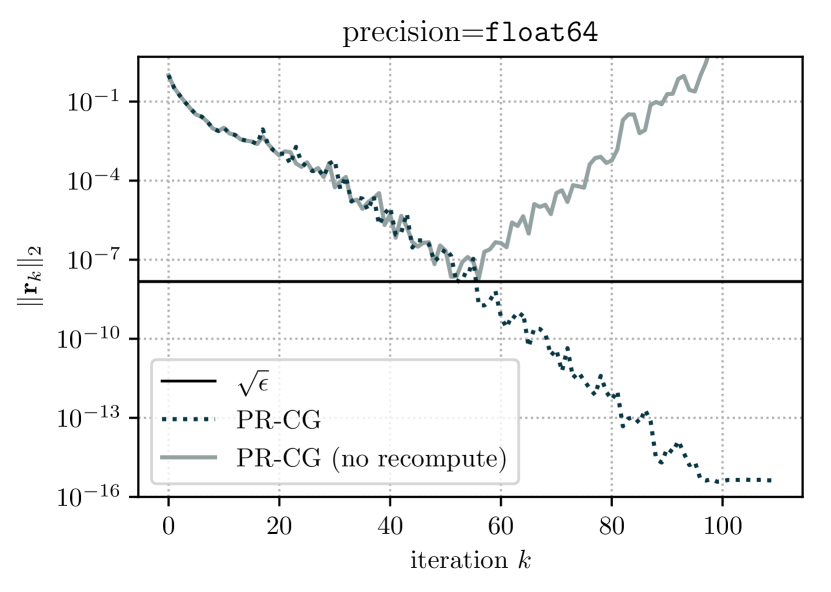
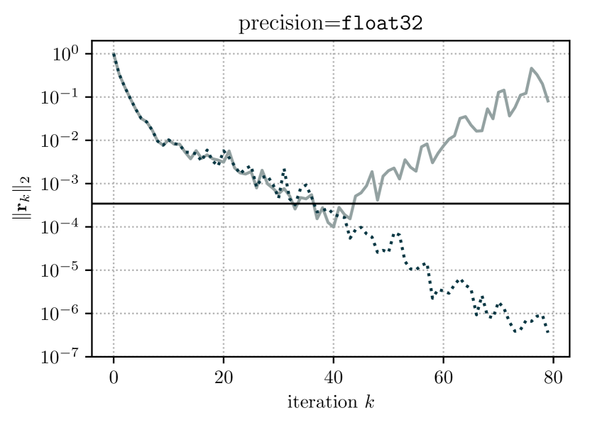
Figure 1: Demonstration, on model_48_8_3 with no preconditioner, of breakdown of PR-CG when $\nu_{k}^{\prime}$ is not recomputed. Breakdown occurs when $\nu_{k}^{\prime}$ becomes negative which can be avoided using the recompute scheme.

We now seek to bound the norms of the quantities $\delta_{\mathbf{r}_{k}}$, $\delta_{\nu_{k-1}}$, $\delta_{\sigma_{k-1}}$, $\delta_{\gamma_{k-1}}$, and $\delta_{\nu^{\prime}_{k}}$. Using Eq. 15, Eq. 18, and the bounds Eq. 12-Eq. 14, and dropping terms of order $O(\epsilon^{2})$, we have

$$\|\delta_{\mathbf{r}_{k}}\| \leq\epsilon\left(\|\mathbf{r}_{k}\|+2|\alpha_{k-1}\|\mathbf{s}_{k-1}\|\right)$$

$$\leq\epsilon\left(\|\mathbf{r}_{k}\|+2|\alpha_{k-1}|\left(\frac{1}{|\alpha_{k-1}|}\left(\|\mathbf{r}_{k-1}\|+\|\mathbf{r}_{k}\|+\|\delta_{\mathbf{r}_{k}}\|\right)\right)\right)$$

$$\leq\epsilon\left(3\|\mathbf{r}_{k}\|+2\|\mathbf{r}_{k-1}\|\right)+2\,\epsilon\,\|\delta_{\mathbf{r}_{k}}\|$$

(19) $$\leq 3\,\epsilon\left(\|\mathbf{r}_{k}\|+\|\mathbf{r}_{k-1}\|\right),$$

(20) $$|\delta_{\nu_{k-1}}| \leq\epsilon\,n\,\|\mathbf{r}_{k-1}\|^{2},$$

$$|\delta_{\sigma_{k-1}}| \leq\epsilon\,n\,\|\mathbf{r}_{k-1}\|\|\mathbf{s}_{k-1}\|$$

$$\leq\epsilon\,n\,\|\mathbf{r}_{k-1}\|\left(\frac{1}{|\alpha_{k-1}|}\left(\|\mathbf{r}_{k-1}\|+\|\mathbf{r}_{k}\|+\|\delta_{\mathbf{r}_{k}}\|\right)\right)$$

(21) $$\leq\epsilon\,n\,\frac{1}{|\alpha_{k-1}|}\left(\|\mathbf{r}_{k-1}\|^{2}+\|\mathbf{r}_{k-1}\|\|\mathbf{r}_{k}\|\right),$$

$$|\delta_{\gamma_{k-1}}| \leq\epsilon\,n\,\|\mathbf{s}_{k-1}\|^{2}$$

(22) $$\leq\epsilon\,n\,\frac{1}{|\alpha_{k-1}|^{2}}\left(\|\mathbf{r}_{k-1}\|+\|\mathbf{r}_{k}\|\right)^{2},$$

$$|\delta_{\nu_{k}^{\prime}}| \leq 3\,\epsilon\left(|\nu_{k-1}|+2|\alpha_{k-1}||\sigma_{k-1}|+|\alpha_{k-1}|^{2}|\gamma_{k-1}|\right)$$

$$\leq 3\,\epsilon\left(\|\mathbf{r}_{k-1}\|^{2}+2|\alpha_{k-1}|\|\mathbf{r}_{k-1}\|\|\mathbf{s}_{k-1}\|+|\alpha_{k-1}|^{2}\|\mathbf{s}_{k-1}\|^{2}\right)$$

$$\leq 3\,\epsilon\left(\|\mathbf{r}_{k-1}\|^{2}+2\|\mathbf{r}_{k-1}\|(\|\mathbf{r}_{k-1}\|+\|\mathbf{r}_{k}\|)+(\|\mathbf{r}_{k-1}\|+\|\mathbf{r}_{k}\|)^{2}\right)$$

$$=3\,\epsilon\left(4\|\mathbf{r}_{k-1}\|^{2}+4\|\mathbf{r}_{k-1}\|\|\mathbf{r}_{k}\|+\|\mathbf{r}_{k}\|^{2}\right).$$

Substituting Eqs. 19, 20, 21, 22, and 3.1 into Eq. 17 gives a bound on the $\nu_{k}^{\prime}$ gap:

(23) $$|\Delta_{\nu_{k}^{\prime}}| \leq\epsilon\left((12+3n)\|\mathbf{r}_{k-1}\|^{2}+(18+4n)\|\mathbf{r}_{k-1}\|\|\mathbf{r}_{k}\|+(9+n)\|\mathbf{r}_{k}\|^{2}\right)$$

(24) $$\leq\epsilon\,(30+7n)\left(\|\mathbf{r}_{k-1}\|^{2}+\|\mathbf{r}_{k}\|^{2}\right).$$

Therefore, given that $\nu^{\prime}_{k}=\|\mathbf{r}_{k}\|^{2}-\Delta_{\nu^{\prime}_{k}}$, it is clear from the above bound that

$$\nu^{\prime}_{k}\geq\|\mathbf{r}_{k}\|^{2}-\epsilon\,(30+7n)\left(\|\mathbf{r}_{k-1}\|^{2}+\|\mathbf{r}_{k}\|^{2}\right)$$

Assuming $\epsilon$ is small enough that the higher order terms do not have an significant impact on the derived bounds, this quantity will remain positive provided $\|\mathbf{r}_{k-1}\|^{2}/\|\mathbf{r}_{k}\|^{2}\leq 1/(\epsilon\,(30+7n))-1$. While we do not explicitly bound $\|\mathbf{r}_{k-1}\|/\|\mathbf{r}_{k}\|$, we note that in practice it is unlikely to be of size $\sim 1/\sqrt{\epsilon n}$, thus explaining why the recompute scheme keeps $\nu_{k}^{\prime}$ positive.

We now consider the case where we do not use the recomputed value $\nu_{k-1}$, i.e., if we were to instead compute

(25) $$\nu_{k}^{\prime}=\nu_{k-1}^{\prime}-2\alpha_{k-1}\sigma_{k-1}+\alpha_{k-1}^{2}\gamma_{k-1}+\underline{\delta}_{\nu_{k}^{\prime}},$$

where $\underline{\delta}_{\nu_{k}^{\prime}}$ represents the local rounding errors in computing this recurrence. In this case we would have, letting $\underline{\Delta}_{\nu_{k}^{\prime}}$ represent the $\nu^{\prime}$-gap without recomputation,

$$\underline{\Delta}_{\nu_{k}^{\prime}} =\langle\mathbf{r}_{k-1},\mathbf{r}_{k-1}\rangle-2\alpha_{k-1}(\sigma_{k-1}-\delta_{\sigma_{k-1}})+\alpha_{k-1}^{2}(\gamma_{k-1}-\delta_{\gamma_{k-1}})$$

$$\phantom{=}+2\langle\delta_{\mathbf{r}_{k}},\mathbf{r}_{k}\rangle-\langle\delta_{\mathbf{r}_{k}},\delta_{\mathbf{r}_{k}}\rangle-\nu_{k-1}^{\prime}+2\alpha_{k-1}\sigma_{k-1}-\alpha_{k-1}^{2}\gamma_{k-1}-\underline{\delta}_{\nu_{k}^{\prime}}$$

$$=(\langle\mathbf{r}_{k-1},\mathbf{r}_{k-1}\rangle-\nu_{k-1}^{\prime})+2\alpha_{k-1}\delta_{\sigma_{k-1}}-\alpha_{k-1}^{2}\delta_{\gamma_{k-1}}+2\langle\delta_{\mathbf{r}_{k}},\mathbf{r}_{k}\rangle-\langle\delta_{\mathbf{r}_{k}},\delta_{\mathbf{r}_{k}}\rangle-\underline{\delta}_{\nu_{k}^{\prime}}$$

$$=\underline{\Delta}_{\nu_{k-1}^{\prime}}+2\alpha_{k-1}\delta_{\sigma_{k-1}}-\alpha_{k-1}^{2}\delta_{\gamma_{k-1}}+2\langle\delta_{\mathbf{r}_{k}},\mathbf{r}_{k}\rangle-\langle\delta_{\mathbf{r}_{k}},\delta_{\mathbf{r}_{k}}\rangle-\underline{\delta}_{\nu_{k}^{\prime}}.$$

Taking the absolute value of both sizes and and ignoring terms of $\mathcal{O}(\epsilon)$, we thus have the bound

(26) $$|\underline{\Delta}_{\nu_{k}^{\prime}}|\leq|\underline{\Delta}_{\nu^{\prime}_{k-1}}|+2|\alpha_{k-1}||\delta_{\sigma_{k-1}}|+\alpha_{k-1}^{2}|\delta_{\gamma_{k-1}}|+2\|\delta_{\mathbf{r}_{k}}\|\|\mathbf{r}_{k}\|+|\underline{\delta}_{\nu_{k}^{\prime}}|.$$

The only term in Eq. 26 that remains to bound is $|\underline{\delta}_{\nu_{k}^{\prime}}|$. From Eq. 25 we have

$$|\underline{\delta}_{\nu_{k}^{\prime}}|\leq 3\,\epsilon\left(|\nu^{\prime}_{k-1}|+2|\alpha_{k-1}||\sigma_{k-1}|+\alpha_{k-1}^{2}\|\gamma_{k-1}\|\right).$$

By definition, $\nu^{\prime}_{k-1}=\|\mathbf{r}_{k-1}\|^{2}-\underline{\Delta}_{\nu^{\prime}_{k-1}}$, so

$$|\underline{\delta}_{\nu_{k}^{\prime}}| \leq 3\,\epsilon\left(\|\mathbf{r}_{k-1}\|^{2}+|\underline{\Delta}_{\nu^{\prime}_{k-1}}|+2|\alpha_{k-1}||\sigma_{k-1}|+\alpha_{k-1}^{2}|\gamma_{k-1}|\right).$$

Thus, using an approach similar to the computation in Section 3.1 we have

(27) $$|\underline{\delta}_{\nu_{k}^{\prime}}|\leq 3\,\epsilon\left(4\|\mathbf{r}_{k-1}\|^{2}+4\|\mathbf{r}_{k-1}\|\|\mathbf{r}_{k}\|+\|\mathbf{r}_{k}\|^{2}+|\underline{\Delta}_{\nu^{\prime}_{k-1}}|\right).$$

Plugging Eq. 27, Eq. 21, Eq. 22, and Eq. 19 into Eq. 26, we obtain

$$|\underline{\Delta}_{\nu_{k}^{\prime}}|\leq(1+3\,\epsilon)|\underline{\Delta}_{\nu_{k-1}^{\prime}}|+\epsilon\,\mathcal{O}(n)\left(\|\mathbf{r}_{k-1}\|^{2}+\|\mathbf{r}_{k}\|^{2}\right).$$

Using that $|\underline{\Delta}_{\nu^{\prime}_{0}}|\leq\epsilon\,n\,\|\mathbf{r}_{0}\|^{2}$, this can be written

(28) $$|\underline{\Delta}_{\nu_{k}^{\prime}}|\leq\epsilon\,\mathcal{O}(n)\sum_{i=0}^{k}\|\mathbf{r}_{i}\|^{2},$$

Thus for the $\nu^{\prime}$-gap without recomputation, we have the bound

(29) $$\nu^{\prime}_{k}\geq\|\mathbf{r}_{k}\|^{2}-\epsilon\,\mathcal{O}(n)\sum_{i=0}^{k}\|\mathbf{r}_{i}\|^{2}.$$

Since now the term subtracted involves the sum of the squares of all previous residuals, which can be large especially at the beginning of the iterations, it is entirely possible that $\nu^{\prime}_{k}$ can become negative at some point during the iterations. While Eq. 29 is only an upper bound, it is more or less clear that this is the cause of instability in the case without recomputation, which explains the observations of Meurant [25]. In fact, if we assume that early residuals have norm $\approx 1$, the form of the expression Eq. 29 suggests that $\nu_{k}^{\prime}$ can no longer be guaranteed to be positive once $\|\mathbf{r}_{k}\|\approx\sqrt{\epsilon}$. This aligns with what we have observed in practice; see for instance Fig. 1.

3.1.1 Maximum attainable accuracy

We now compute an expression for the residual gap in Algorithm 2. Substituting in our recurrences for $\mathbf{x}_{k}$ and $\mathbf{r}_{k}$ computed in finite precision, we find

$$\Delta_{\mathbf{r}_{k}} =\mathbf{b}-\mathbf{A}(\mathbf{x}_{k-1}+\alpha_{k-1}\mathbf{p}_{k-1}+\delta_{\mathbf{x}_{k}})-(\mathbf{r}_{k-1}-\alpha_{k-1}\mathbf{s}_{k-1}+\delta_{\mathbf{r}_{k}})$$

$$=(\mathbf{b}-\mathbf{A}\mathbf{x}_{k-1}-\mathbf{r}_{k-1})+\alpha_{k-1}(\mathbf{s}_{k-1}-A\mathbf{p}_{k-1})-\mathbf{A}\delta_{\mathbf{x}_{k}}-\delta_{\mathbf{r}_{k}}$$

$$=\Delta_{\mathbf{r}_{k-1}}+\alpha_{k-1}\delta_{\mathbf{s}_{k-1}}-\mathbf{A}\delta_{\mathbf{x}_{k}}-\delta_{\mathbf{r}_{k}}.$$

Therefore the residual gap can be written

$$\Delta_{\mathbf{r}_{k}}=\Delta_{\mathbf{r}_{0}}+\sum_{i=1}^{k}\left(\alpha_{i-1}\delta_{\mathbf{s}_{i-1}}-\mathbf{A}\delta_{\mathbf{x}_{i}}-\delta_{\mathbf{r}_{i}}\right).$$

This expression is a simple accumulation of local rounding errors. We note that the residual gaps for HS-CG and CG-CG are both given by

$$\Delta_{\mathbf{r}_{k}}=\Delta_{\mathbf{r}_{0}}-\sum_{i=1}^{k}\left(\mathbf{A}\delta_{\mathbf{x}_{i}}+\delta_{\mathbf{r}_{i}}\right),$$

where the $\delta_{\text{quantity}}$ terms correspond to the round off errors made by those algorithms respectively [8].

3.1.2 Towards understanding convergence

We now derive an expression for the extent to which the recurrence Eq. 9 is satisfied by PR-CG in finite precision. We express $\mathbf{s}_{k}=\mathbf{A}\mathbf{p}_{k}+\delta_{\mathbf{s}_{k}}$ in terms of $\mathbf{r}_{k}$ and $\mathbf{s}_{k-1}$, writing

$$\mathbf{s}_{k} =\mathbf{A}(\mathbf{r}_{k}+\beta_{k}\mathbf{p}_{k-1}+\delta_{\mathbf{p}_{k}})+\delta_{\mathbf{s}_{k}}$$

$$=\mathbf{A}\mathbf{r}_{k}+\beta_{k}\mathbf{A}\mathbf{p}_{k-1}+\mathbf{A}\delta_{\mathbf{p}_{k}}+\delta_{\mathbf{s}_{k}}$$

(30) $$=\mathbf{A}\mathbf{r}_{k}+\beta_{k}(\mathbf{s}_{k-1}-\delta_{\mathbf{s}_{k-1}})+\mathbf{A}\delta_{\mathbf{p}_{k}}+\delta_{\mathbf{s}_{k}}.$$

By rearranging the equation $\mathbf{r}_{k}=\mathbf{r}_{k-1}-\alpha_{k-1}\mathbf{s}_{k-1}+\delta_{\mathbf{r}_{k}}$, we can write $\mathbf{s}_{k-1}=(1/\alpha_{k-1})(\mathbf{r}_{k-1}-\mathbf{r}_{k}+\delta_{\mathbf{r}_{k}})$. From this we compute

$$\mathbf{s}_{k}-\beta_{k}\mathbf{s}_{k-1} =\frac{1}{\alpha_{k}}\left(\mathbf{r}_{k}-\mathbf{r}_{k+1}+\delta_{\mathbf{r}_{k+1}}\right)-\frac{\beta_{k}}{\alpha_{k-1}}\left(\mathbf{r}_{k-1}-\mathbf{r}_{k}+\delta_{\mathbf{r}_{k}}\right)$$

$$=-\frac{1}{\alpha_{k}}\mathbf{r}_{k+1}+\left(\frac{1}{\alpha_{k}}+\frac{\beta_{k}}{\alpha_{k-1}}\right)\mathbf{r}_{k}-\frac{\beta_{k}}{\alpha_{k-1}}\mathbf{r}_{k-1}+\frac{1}{\alpha_{k}}\delta_{\mathbf{r}_{k+1}}-\frac{\beta_{k}}{\alpha_{k-1}}\delta_{\mathbf{r}_{k}}.$$

Thus, shifting the indexing down by one, Eq. 30 becomes

(31) $$\mathbf{A}\mathbf{r}_{k-1} =-\frac{1}{\alpha_{k-1}}\mathbf{r}_{k}+\left(\frac{1}{\alpha_{k-1}}+\frac{\beta_{k-1}}{\alpha_{k-2}}\right)\mathbf{r}_{k-1}-\frac{\beta_{k-1}}{\alpha_{k-2}}\mathbf{r}_{k-2}+\mathbf{f}_{k},$$

where

$$\mathbf{f}_{k} =-\frac{\beta_{k-1}}{\alpha_{k-2}}\delta_{\mathbf{r}_{k-1}}+\beta_{k-1}\delta_{\mathbf{s}_{k-2}}-\mathbf{A}\delta_{\mathbf{p}_{k-1}}-\delta_{\mathbf{s}_{k-1}}+\frac{1}{\alpha_{k-1}}\delta_{\mathbf{r}_{k}}.$$

Defining $\mathbf{q}_{k+1}:=(-1)^{k}\mathbf{r}_{k}/\|\mathbf{r}_{k}\|$ we obtain the three-term recurrence

(32) $$\mathbf{A}\mathbf{q}_{k} =\frac{1}{\alpha_{k-1}}\frac{\|\mathbf{r}_{k}\|}{\|\mathbf{r}_{k-1}\|}\mathbf{q}_{k+1}+\left(\frac{1}{\alpha_{k-1}}+\frac{\beta_{k-1}}{\alpha_{k-2}}\right)\mathbf{q}_{k}+\frac{\beta_{k-1}}{\alpha_{k-2}}\frac{\|\mathbf{r}_{k-2}\|}{\|\mathbf{r}_{k-1}\|}\mathbf{q}_{k-1}-\frac{(-1)^{k-1}}{\|\mathbf{r}_{k-1}\|}\mathbf{f}_{k}.$$

In order for Greenbaum’s analysis to apply, we must write this as a symmetric three-term recurrence with some perturbation term. Using our definition of the $\nu^{\prime}$-gap, $\Delta_{\nu_{k}^{\prime}}:=\langle\mathbf{r}_{k},\mathbf{r}_{k}\rangle-\nu_{k}^{\prime}$, we have

$$\beta_{k} =\frac{\nu_{k}^{\prime}}{\nu_{k-1}}+\delta_{\beta_{k}}=\frac{\|\mathbf{r}_{k}\|^{2}+\Delta_{\nu_{k}^{\prime}}}{\|\mathbf{r}_{k-1}\|^{2}+\delta_{\nu_{k-1}^{\prime}}}+\delta_{\beta_{k}}=\frac{\|\mathbf{r}_{k}\|^{2}}{\|\mathbf{r}_{k-1}\|^{2}}+\Delta_{\beta_{k}},$$

where $\Delta_{\beta_{k}}:=\beta_{k}-\|\mathbf{r}_{k}\|^{2}/\|\mathbf{r}_{k-1}\|^{2}$ can be written explicitly as

$$\Delta_{\beta_{k}}=\frac{\Delta_{\nu_{k}^{\prime}}+\|\mathbf{r}_{k-1}\|^{2}\delta_{\beta_{k}}+\delta_{\nu_{k-1}^{\prime}}\delta_{\beta_{k}}}{\|\mathbf{r}_{k-1}\|^{2}+\delta_{\nu_{k-1}^{\prime}}}+\frac{-\|\mathbf{r}_{k}\|^{2}\delta_{\nu_{k-1}^{\prime}}}{\|\mathbf{r}_{k-1}\|^{2}(\|\mathbf{r}_{k-1}\|^{2}+\delta_{\nu_{k-1}^{\prime}})}.$$

Then, by plugging this expression for $\beta_{k-1}$ into Eq. 32, we obtain the approximately symmetric three-term recurrence for $\mathbf{q}_{k}$,

$$\mathbf{A}\mathbf{q}_{k} =\frac{1}{\alpha_{k-1}}\frac{\|\mathbf{r}_{k}\|}{\|\mathbf{r}_{k-1}\|}\mathbf{q}_{k+1}+\left(\frac{1}{\alpha_{k-1}}+\frac{\beta_{k-1}}{\alpha_{k-2}}\right)\mathbf{q}_{k}+\frac{1}{\alpha_{k-2}}\frac{\|\mathbf{r}_{k-1}\|}{\|\mathbf{r}_{k-2}\|}\mathbf{q}_{k-1}+\mathbf{F}_{k},$$

so that the error in the three-term Lanczos recurrence is given by

$$\mathbf{F}_{k} =\frac{\Delta_{\beta_{k-1}}}{\alpha_{k-2}}\frac{\|\mathbf{r}_{k-2}\|^{2}}{\|\mathbf{r}_{k-1}\|^{2}}\mathbf{q}_{k-1}-\frac{(-1)^{k}}{\|\mathbf{r}_{k-1}\|}\mathbf{f}_{k}.$$

Hence, the amount by which the updated residuals in PR-CG fail to satisfy Eq. 9 depends only on local rounding errors, which was also observed for HS-CG and CG-CG in [20]. While $\|\mathbf{r}_{k-1}\|$ may become quite small, we note that $\mathbf{f}_{k}$ consists of roundoff errors made in iterations $k-1$ and $k-2$ and corresponds to vectors which are of comparable size to $\mathbf{r}_{k-1}$; i.e., it is reasonable to assume that the ratio of the norms of these vectors to $\mathbf{r}_{k-1}$ will be much less than $1/\epsilon$. Based on this heuristic, $\mathbf{f}_{k}/\|\mathbf{r}_{k-1}\|$ can be expected to stay small, which provides some indication for why the rate of convergence of PR-CG tends to be similar to HS-CG and CG-CG.

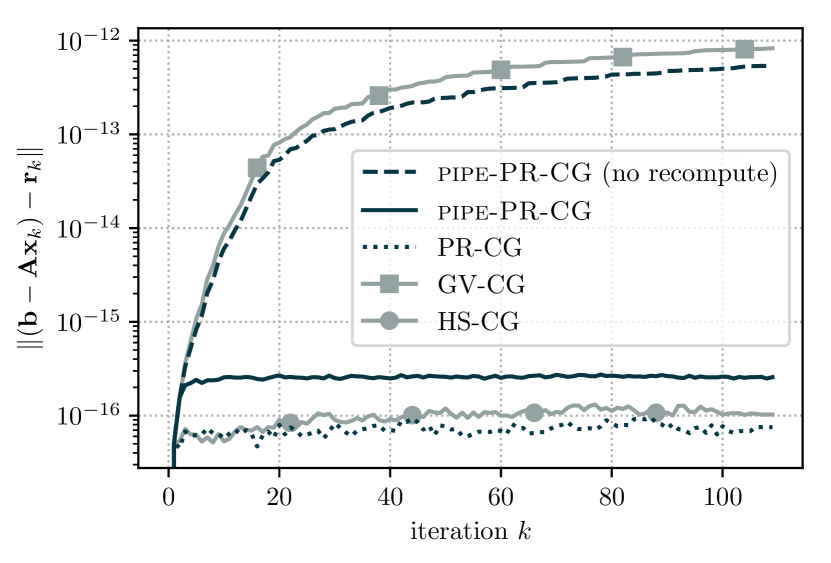
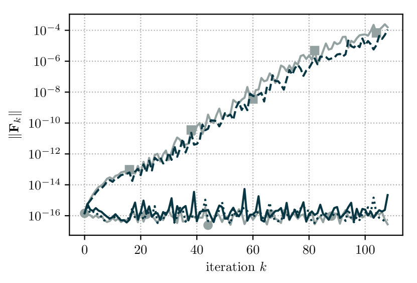
Figure 2: Residual gap (lefT) and 2-norm of error in three-term Lanczos recurrence (right) on model_48_8_3 without a preconditioner. In the legend, “no recompute” indicates that $\mathbf{w}_{k}$ is not recomputed.

3.2 Pipelined predict-and-recompute CG

We now provide for pipe-PR-CG a similar rounding error analysis for the residual gap and Lanczos recurrence as we did for PR-CG. Of course, the $\delta_{\text{quantity}}$ error terms in this section are different from those in the previous section, even though we use many of the same symbols for notational convenience. In particular, our expression for $\mathbf{s}_{k}$ in finite precision is now $\mathbf{s}_{k}=\mathbf{w}^{\prime}_{k}+\beta_{k}\mathbf{s}_{k-1}+\delta_{\mathbf{s}_{k}}$ and we add the recurrences

$$\mathbf{w}^{\prime}_{k} =\mathbf{w}_{k-1}-\alpha_{k-1}\mathbf{u}_{k-1}+\delta_{\mathbf{w}^{\prime}_{k}}, \mathbf{w}_{k} =\mathbf{A}\mathbf{r}_{k}+\delta_{\mathbf{w}_{k}},$$

$$\mathbf{p}_{k} =\mathbf{r}_{k}+\beta_{k}\mathbf{p}_{k-1}+\delta_{\mathbf{p}_{k}}, \mathbf{u}_{k} =\mathbf{A}\mathbf{s}_{k}+\delta_{\mathbf{u}_{k}}.$$

We note that the same expression holds for $\Delta_{\nu_{k}^{\prime}}$ as with PR-CG; see Eq. 16.

3.2.1 Maximum attainable accuracy

Similarly as for PR-CG, we can write the residual gap in pipe-PR-CG as

$$\Delta_{\mathbf{r}_{k}} =\mathbf{b}-\mathbf{A}\mathbf{x}_{k}-\mathbf{r}_{k}$$

$$=\Delta_{\mathbf{r}_{k-1}}+\alpha_{k-1}(\mathbf{s}_{k-1}-\mathbf{A}\mathbf{p}_{k-1})-\mathbf{A}\delta_{\mathbf{x}_{k}}-\delta_{\mathbf{r}_{k}}$$

$$=\Delta_{\mathbf{r}_{k-1}}-\alpha_{k-1}\Delta_{\mathbf{s}_{k-1}}-\mathbf{A}\delta_{\mathbf{x}_{k}}-\delta_{\mathbf{r}_{k}}$$

$$=\Delta_{\mathbf{r}_{0}}-\sum_{i=1}^{k}\left[\alpha_{i-1}\Delta_{\mathbf{s}_{i-1}}+\mathbf{A}\delta_{\mathbf{x}_{i}}+\delta_{\mathbf{r}_{i}}\right],$$

where $\Delta_{\mathbf{s}_{i}}:=\mathbf{A}\mathbf{p}_{i}-\mathbf{s}_{i}$ represents the gap between $\mathbf{A}\mathbf{p}_{i}$ and the recursively-computed quantity $\mathbf{s}_{i}$. We can write this $\mathbf{s}$-gap as

$$\Delta_{\mathbf{s}_{i}} =\mathbf{A}(\mathbf{r}_{i}+\beta_{i}\mathbf{p}_{i-1}+\delta_{\mathbf{p}_{i}})-(\mathbf{w}_{i}^{\prime}+\beta_{i}\mathbf{s}_{i-1}+\delta_{\mathbf{s}_{i}})$$

$$=(\mathbf{A}\mathbf{r}_{i}-\mathbf{w}_{i}^{\prime})+\beta_{i}(A\mathbf{p}_{i-1}-\mathbf{s}_{i-1})+\mathbf{A}\delta_{\mathbf{p}_{i}}-\delta_{\mathbf{s}_{i}}$$

$$=\Delta_{\mathbf{w}_{i}^{\prime}}+\beta_{i}\Delta_{\mathbf{s}_{i-1}}+\mathbf{A}\delta_{\mathbf{p}_{i}}-\delta_{\mathbf{s}_{i}}$$

$$=\Delta_{\mathbf{s}_{0}}\prod_{j=1}^{i}\beta_{j}+\sum_{j=1}^{i}\Bigg{[}(\Delta_{\mathbf{w}_{j}^{\prime}}+\mathbf{A}\delta_{\mathbf{p}_{j}}-\delta_{\mathbf{s}_{j}})\prod_{\ell=j+1}^{i}\beta_{\ell}\Bigg{]},$$

where $\Delta_{\mathbf{w}_{j}^{\prime}}$ denotes the gap $\Delta_{\mathbf{w}_{j}^{\prime}}:=\mathbf{A}\mathbf{r}_{j}-\mathbf{w}_{j}^{\prime}$. Now we look at how to bound this $\mathbf{w^{\prime}}$-gap. In pipe-PR-CG, we have

$$\Delta_{\mathbf{w}_{j}^{\prime}} =\mathbf{A}(\mathbf{r}_{j-1}-\alpha_{j-1}\mathbf{s}_{j-1}+\delta_{\mathbf{r}_{j}})-(\mathbf{w}_{j-1}-\alpha_{j-1}\mathbf{u}_{j-1}+\delta_{\mathbf{w}_{j}^{\prime}})$$

$$=\mathbf{A}\mathbf{r}_{j-1}-\mathbf{w}_{j-1}-\alpha_{j-1}(\mathbf{A}\mathbf{s}_{j-1}-\mathbf{u}_{j-1})-\delta_{\mathbf{w}_{k}^{\prime}}+\mathbf{A}\delta_{\mathbf{r}_{j}}$$

(33) $$=-\delta_{\mathbf{w}_{j-1}}+\alpha_{j-1}\delta_{\mathbf{u}_{j-1}}-\mathbf{A}\delta_{\mathbf{r}_{j}}-\delta_{\mathbf{w}_{j}^{\prime}},$$

which is the sum of local rounding errors.

Notice that without recomputation, i.e., if we were to instead compute

$$\mathbf{w}_{j}^{\prime}-\mathbf{w}_{j-1}^{\prime}-\alpha_{j-1}\mathbf{u}_{j-1}+\underline{\delta}_{\mathbf{w}_{j}^{\prime}},$$

where $\underline{\delta}_{\mathbf{w}_{j}^{\prime}}$ denotes the local rounding errors in computing this recurrence, then we would have, letting $\underline{\Delta}_{\mathbf{w}_{j}^{\prime}}$ denote the $\mathbf{w}^{\prime}$-gap in the case of no recomputation,

$$\underline{\Delta}_{\mathbf{w}_{j}^{\prime}} =\mathbf{A}\mathbf{r}_{j-1}-\mathbf{w}_{j-1}^{\prime}-\alpha_{j-1}(\mathbf{A}\mathbf{s}_{j-1}-\mathbf{u}_{j-1})+\mathbf{A}\delta_{\mathbf{r}_{j}}-\underline{\delta}_{\mathbf{w}_{j}^{\prime}}$$

$$=\underline{\Delta}_{\mathbf{w}_{j-1}^{\prime}}+\alpha_{j-1}\delta_{\mathbf{u}_{j-1}}+A\delta_{\mathbf{r}_{j}}-\underline{\delta}_{\mathbf{w}_{j}^{\prime}}$$

(34) $$=\underline{\Delta}_{\mathbf{w}_{0}^{\prime}}+\sum_{\ell=1}^{j}\left[\alpha_{\ell-1}\delta_{\mathbf{u}_{\ell-1}}+\mathbf{A}\delta_{\mathbf{r}_{\ell}}+\delta_{\mathbf{w}_{\ell}^{\prime}}\right].$$

Thus, comparing Eq. 33 with Eq. 34, we see that if we use recomputation, $\Delta_{\mathbf{w}_{j}^{\prime}}$ is essentially “reset” in each iteration; the errors made do not accumulate and $\Delta_{\mathbf{w}_{j}^{\prime}}$ remains a small multiple of the machine precision. Without recomputation, however, a bound on size of the quantity $\underline{\Delta}_{\mathbf{w}_{j}^{\prime}}$ will be monotonically increasing, growing larger in each iteration due to the accumulation of rounding errors. We note that the expression for the maximum attainable accuracy for pipe-PR-CG in Eq. 34, without the recomputation of $\mathbf{w}_{j}$, closely resembles the expression derived for the maximum attainable accuracy for GV-CG derived in [8]. This is demonstrated numerically in Fig. 2. Indeed, without recomputation, it is easily observed that pipe-PR-CG and GV-CG typically behave quite similarly.

If we look at the expression for $\Delta_{\mathbf{s}_{i}}$, we see that $\Delta_{\mathbf{w}_{j}^{\prime}}$ (or in the case of no recomputation, $\underline{\Delta}_{\mathbf{w}_{j}^{\prime}}$), along with local rounding errors $\mathbf{A}\delta_{\mathbf{p}_{j}}$ and $\delta_{\mathbf{s}_{j}}$, is amplified by a product of $\beta$ terms, $\prod_{\ell=j+1}^{i}\beta_{\ell}$. In exact arithmetic at least, we have

$$\prod_{\ell=j+1}^{i}\beta_{\ell}=\beta_{j+1}\beta_{j+2}\cdots\beta_{i}=\frac{\|\mathbf{r}_{i}\|^{2}}{\|\mathbf{r}_{j}\|^{2}},$$

and we expect this quantity to be greater than one in cases where CG exhibits large oscillation in the residual norm.

Thus it is clear why recomputation can improve the maximal attainable accuracy: the term $\Delta_{\mathbf{w}_{j}^{\prime}}$ should remain small (some multiple of $\epsilon$) in this case, whereas without recomputation, the analogous term can grow larger and larger throughout the iterations. It is also clear why the pipe-PR-CG method can exhibit potentially decreased accuracy versus the HS-CG method; the local rounding errors (including the term $\Delta_{\mathbf{w}_{j}^{\prime}}$) are amplified by quantities related to the ratios of residual norms, which can be large for certain problems.

Finally, we note that the same theory holds for pipe-M-CG as the expressions for the relevant recurrences are the same as in pipe-PR-CG.

3.2.2 Towards understanding convergence

Following the same procedure as for PR-CG, we can write

$$\mathbf{s}_{k} =\mathbf{w}_{k}^{\prime}+\beta_{k}\mathbf{s}_{k-1}+\delta_{\mathbf{s}_{k}}=\mathbf{A}\mathbf{r}_{k}+\beta_{k}\mathbf{s}_{k-1}-\Delta_{\mathbf{w}_{k}^{\prime}}+\delta_{\mathbf{s}_{k}}.$$

This is almost the same as Eq. 30 except that $\mathbf{A}\delta_{\mathbf{p}_{k}}-\beta_{k}\delta_{\mathbf{s}_{k-1}}$ has been replaced by $-\Delta_{\mathbf{w}_{k}^{\prime}}$. Thus, through similar computations as above, we find

$$\mathbf{A}\mathbf{q}_{k} =\frac{1}{\alpha_{k-1}}\frac{\|\mathbf{r}_{k}\|}{\|\mathbf{r}_{k-1}\|}\mathbf{q}_{k+1}+\left(\frac{1}{\alpha_{k-1}}+\frac{\beta_{k-1}}{\alpha_{k-2}}\right)\mathbf{q}_{k}+\frac{1}{\alpha_{k-2}}\frac{\|\mathbf{r}_{k-1}\|}{\|\mathbf{r}_{k-2}\|}\mathbf{q}_{k-1}+\mathbf{F}_{k},$$

where there error term is given by

$$\mathbf{F}_{k} =\frac{\Delta_{\beta_{k-1}}}{\alpha_{k-2}}\frac{\|\mathbf{r}_{k-2}\|^{2}}{\|\mathbf{r}_{k-1}\|^{2}}\mathbf{q}_{k-1}-\frac{(-1)^{k}}{\|\mathbf{r}_{k-1}\|}\mathbf{f}_{k}$$

and

$$\mathbf{f}_{k} =-\frac{\beta_{k-1}}{\alpha_{k-2}}\delta_{\mathbf{r}_{k-1}}+\Delta_{\mathbf{w}_{k}^{\prime}}-\delta_{\mathbf{s}_{k-1}}+\delta_{\mathbf{r}_{k}}.$$

While the three-term Lanczos recurrence generated by pipe-PR-CG is satisfied to within local rounding errors, the error term $\mathbf{F}_{k}$ for pipe-PR-CG depends on $\Delta_{w_{k}^{\prime}}$ rather than $\mathbf{A}\delta_{\mathbf{p}_{k}}$. Thus, it is reasonable to expect it to be larger than the error term for PR-CG. On the other hand, the expression for the degree to which GV-CG satisfies the three-term Lanczos recurrence depends on errors made in all previous steps [20]. This provides some intuition for why the rate of convergence of pipe-PR-CG is observed to be better than GV-CG. Again, a numerical comparison is shown in Fig. 2.

4 Numerical experiments

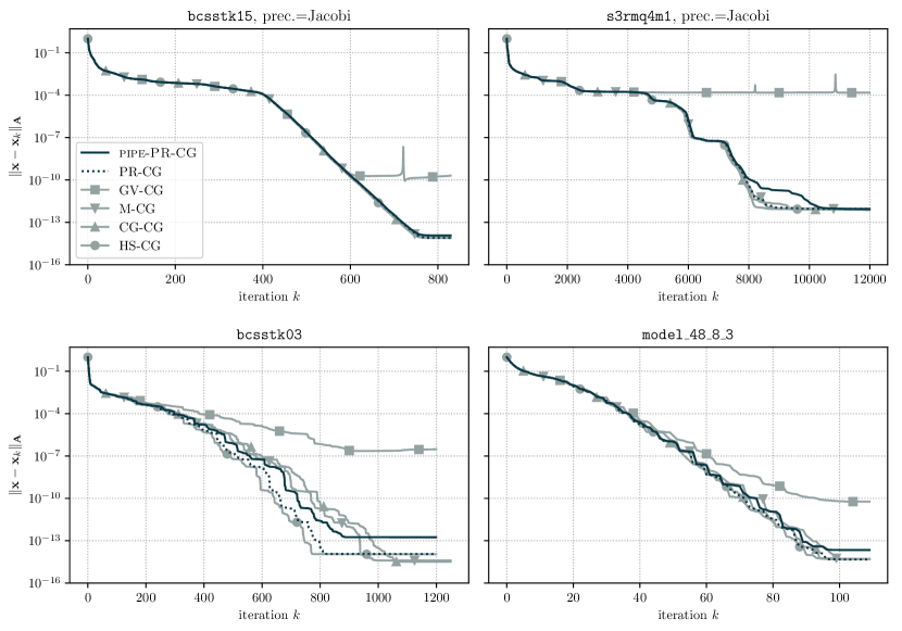
Figure 3: Error $\mathbf{A}$-norm of conjugate gradient variants on selected problems.

In this section we present the results of numerical experiments intended to give insight into the numerical behavior of the variants introduced in this paper. We run experiments on a range of matrices from the Matrix Market [3]. In addition we include a model problem which was introduced in [34] and has since been considered in [35, 12, 20]. This model problem has eigenvalues $\lambda_{1}=1/\kappa$, $\lambda_{n}=1$, and for $i=2,3,\ldots,n-1$,

(35) $$\lambda_{i}=\lambda_{1}+\left(\frac{i-1}{n-1}\right)\cdot(\lambda_{n}-\lambda_{1})\cdot\rho^{n-i}$$

for $n=48$, $\rho=0.8$, and $\kappa=10^{3}$, with eigenvectors chosen uniformly from the set of unitary matrices. Since the spacing between eigenvalues grows exponentially, this is a particularly difficult problem in finite precision arithmetic.

The experiments are implemented in NumPy using IEEE double precision floating point arithmetic. The results are outlined in LABEL:table:convergence. In this table we give two summary statistics: (i) the number of iterations required to decrease the $\mathbf{A}$-norm of the error by a factor of $10^{5}$, and (ii) the minimum error reached. For a given problem, these two quantities give a rough indication of the rate of convergence and ultimately attainable accuracy. Plots of convergence for all experiments appearing in LABEL:table:convergence can be found online in the repository linked in Appendix A. As was done in [16], the right-hand side $\mathbf{b}$ is chosen so that $\mathbf{x}^{*}=\mathbf{A}^{-1}\mathbf{b}$ has entries $1/\sqrt{n}$, and the initial guess $\mathbf{x}_{0}$ is the zero vector. For most problems we selected, we run tests without a preconditioner, and then with a simple Jacobi (diagonal) preconditioner. For each problem, we run all variants for a sufficient number of iterations such that the true residual stagnates.

Fig. 3 shows the results of four of the numerical tests contained in LABEL:table:convergence. These problems were chosen to highlight some of the types of behavior observed for finite precision CG variants. On some problems such as bcsstk03 and the model problem model_48_8_3, the rate of convergence and final accuracy of each variant may differ, due primarily to the large gaps in the spectrum [4]. Alternatively, on many other problems, such as bcsstk15 with Jacobi preconditioning, the rate of convergence for all variants is the same until the final accuracy is reached. However, even on such problems, it may be possible for the final accuracy of a variant to be significantly worse than other variants. For instance, on s3rmq4m1 with Jacobi preconditioning, the final accuracy of GV-CG is 8 orders of magnitude worse than HS-CG even though the rates of convergence are initially the same.

We note that on problems where CG-CG encounters a delay of convergence, such as bcsstk03, PR-CG converges more quickly. More notably, for the experiments in LABEL:table:convergence, the pipelined predict-and-recompute variants pipe-M-CG and pipe-PR-CG show significantly better convergence than GV-CG, frequently exhibiting convergence similar to that of HS-CG. In particular, on all the problems tested, pipe-M-CG and pipe-PR-CG converge to a final accuracy within 10 percent (on a log scale) of that of HS-CG if Jacobi preconditioning is used, and on some problems, these two variants actually converge to a better final accuracy than HS-CG.

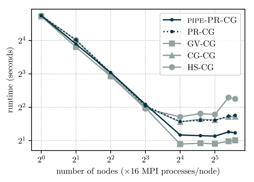
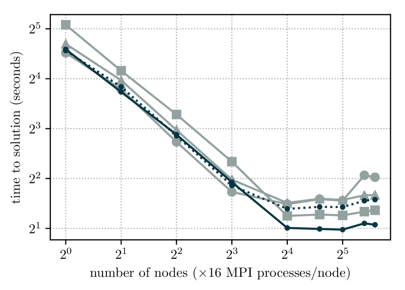
Figure 4: Strong scaling experiment on (dense) model problem with $n=10752$ unknowns and $1000$ iterations. Time to solution is approximate time to decrease the $\mathbf{A}$-norm of error by a factor of $10^{5}$.

5 Parallel performance

We implement the unpreconditioned variants discussed in this paper using mpi4py [11] and perform a strong scaling experiment on the Hyak supercomputer at the University of Washington. In this experiment we solve the model problem Eq. 35 with parameters $n=10752$, $\rho=0.9$, $\kappa=10^{6}$. In order to demonstrate that the additional computation costs associated with the extra matrix-vector product required by pipe-PR-CG are not particularly important, we represent our model problem as a dense matrix. In each trial, we first allocate 48 nodes with 16 processors each and then iterate over a selection of node counts. On each node count we run each variant with for $1000$ iterations timing only the main loop of each variant and not any costs corresponding to setup. In order to account for effects such as cluster topology and system noise we repeat this process 4 times and report the minimum runtimes and accuracy of these runs.

Figure 4 shows the results of the experiment. In our implementation, we compute $\mathbf{A}\mathbf{s}_{k}$ and $\mathbf{A}\mathbf{r}_{k}$ simultaneously using a block vector $[\mathbf{s}_{k},\mathbf{r}_{k}]$ so that $\mathbf{A}$ is accessed only once per iteration. While the number of floating point operations is nearly doubled in pipe-PR-CG, the memory access pattern is more or less unchanged. Specifically, $\mathbf{A}$ needs to only be read/communicated a single time per iteration. For this reason, the runtime of pipe-PR-CG is almost the same as GV-CG. If we compute the two matrix products separately, then the runtime of pipe-PR-CG is approximately doubled on low node counts.

In both cases, as a higher number of nodes are used, and communication costs begin to come into play, pipe-PR-CG becomes faster than the non-pipelined variants and exhibits similar scaling properties as GV-CG. In the high node limit, GV-CG does perform marginally better than pipe-PR-CG. This is because our test involves a dense matrix, so due to the two matrix-vector products, the amount of data communicated between nodes in pipe-PR-CG is nearly double that of GV-CG. However, it is important to keep in mind that the actual “time to solution” is given by the product of the time per iteration and the number of iterations required.

6 Future work

First, while we have provided an analysis of the maximal attainable accuracy for our new variants, the analysis of the resulting convergence rate is far from complete. This is a difficult area of study and deserves further rigorous treatment.

Second, since the maximum reduction in communication cost of pipe-PR-CG over HS-CG is only a factor of three, potential ways of further decreasing communication costs should be explored. Recently, there has been work on “deep pipelined” CG variants where more matrix-vector products are overlapped with global communication; see, for instance, [16, 10, 7]. This approach is similar to the “look ahead” strategy suggested in [30] and may be compatible with the schemes introduced here.

Alternatively, it may be possible to either incorporate predict-and-recompute strategies into $s$-step methods or to develop new $s$-step methods which are built on PR-CG. As CG-CG is the $s=1$ case of the $s$-step method from [6], we expect it may be possible to develop an $s$-step method based based on PR-CG which has slightly better numerical properties than CG-CG. Finding such a method which is usable in practice would be of great practical interest.

Finally, the predict-and-recompute variants presented here can be naturally extended to other related methods such as conjugate residual and conjugate gradient squared.

7 Conclusion

In this paper we extend the predict-and-recompute idea of Meurant [25] and derive new pipelined CG variants, pipe-M-CG and pipe-PR-CG. These variants exhibit better theoretical scaling properties than the standard HS-CG algorithm as well as improved numerical behavior compared to their previously-studied counterpart, GV-CG, on every numerical experiment we ran. We provide an analysis of the maximum attainable accuracy, applicable to both pipe-M-CG and pipe-PR-CG, which explains the benefit of the predict-and-recompute with regards to avoiding the breakdown observed in [25], as well as to the improved final accuracy and rate of convergence observed by our pipelined variants. We additionally provide a strong scaling experiment which confirms the potential performance benefits of our approach. Our predict-and-recompute variants require exactly the same input parameters as HS-CG, and therefore have the potential to be used wherever HS-CG is used without any additional parameter selection. Despite these advances, there is still significant room for future work on high performance CG variants, especially in the direction of further decreasing the communication costs.

Appendix A Additional resources

A repository with the code necessary to reproduce all of the figures and results in this paper is available at https://github.com/tchen01/new_cg_variants, and released to the public domain under the MIT License. The repository also contains convergence data and plots for all the matrices listed in LABEL:table:convergence.

We are committed to facilitating the reproducibility process, and encourage questions and inquiries into the methods used in this paper.

Appendix B Bound on sum of products

Define

$$C=\sum_{i=1}^{n}\prod_{j=1}^{b_{i}}c_{i,j}.$$

Then

$$\left|\operatorname{fp}\left(\prod_{j=1}^{b_{i}}c_{i,j}\right)-\prod_{j=1}^{b_{i}}c_{i,j}\right|\leq(1+\epsilon)^{b_{i}}\prod_{j=1}^{b_{i}}\left|c_{i,j}\right|,$$

so

(36) $$|\operatorname{fp}(C)-C|\leq n\,\epsilon\sum_{i=1}^{n}(1+\epsilon)^{b_{i}}\prod_{j=1}^{b_{i}}|c_{i,j}|=n\,\epsilon\sum_{i=1}^{n}\prod_{j=1}^{b_{i}}|c_{i,j}|+\mathcal{O}(\epsilon^{2}).$$

Appendix C A note on other variants studied

Many of the scalar quantities appearing in the variants discussed in this paper can be replaced with equivalent expressions. For instance, the difference between M-CG and PR-CG (as well as pipe-M-CG and pipe-PR-CG) is the choice of expression for $\nu_{k}$, which in exact arithmetic is equal to $\langle\tilde{\mathbf{r}}_{k},\mathbf{r}_{k}\rangle$. However, it is not typically clear which scalar expression should be used.

We first discuss our simplified expression for Eq. 2 which is used in PR-CG and pipe-PR-CG. Recall that in exact arithmetic, $\langle\tilde{\mathbf{s}}_{k},\mathbf{r}_{k}\rangle=\langle\mathbf{s}_{k},\tilde{\mathbf{r}}_{k}\rangle$. This cannot be expected to be true in finite precision.

Writing the finite precision recurrences

$$\tilde{\mathbf{s}}_{k} =\mathbf{M}^{-1}\mathbf{s}_{k}+\delta_{\tilde{\mathbf{s}}_{k}}, \tilde{\mathbf{r}}_{k} =\tilde{\mathbf{r}}_{k-1}-\alpha_{k-1}\tilde{\mathbf{s}}_{k-1}+\delta_{\tilde{\mathbf{r}}_{k}},$$

we have

$$\langle\tilde{\mathbf{s}}_{k},\mathbf{r}_{k}\rangle =\langle\mathbf{M}^{-1}\mathbf{s}_{k}+\delta_{\tilde{\mathbf{s}}_{k}},\mathbf{r}_{k}\rangle$$

$$=\langle\mathbf{s}_{k},\mathbf{M}^{-1}\mathbf{r}_{k}\rangle+\langle\delta_{\tilde{\mathbf{s}}_{k}},\mathbf{r}_{k}\rangle$$

$$=\langle\mathbf{s}_{k},\tilde{\mathbf{r}}_{k}\rangle+\langle\mathbf{s}_{k},\Delta_{\tilde{\mathbf{r}}_{k}}\rangle+\langle\delta_{\tilde{\mathbf{s}}_{k}},\mathbf{r}_{k}\rangle,$$

where we have defined the $\tilde{\mathbf{r}}$-gap as $\Delta_{\tilde{\mathbf{r}}_{k}}:=\mathbf{M}^{-1}\mathbf{r}_{k}-\tilde{\mathbf{r}}_{k}$. For the $\tilde{\mathbf{r}}$-gap, we have

$$\Delta_{\tilde{\mathbf{r}}_{k}} =\mathbf{M}^{-1}(\mathbf{r}_{k-1}-\alpha_{k-1}\mathbf{s}_{k-1}+\delta_{\mathbf{r}_{k}})-(\tilde{\mathbf{r}}_{k-1}-\alpha_{k-1}\tilde{\mathbf{s}}_{k-1}+\delta_{\tilde{\mathbf{r}}_{k}})$$

$$=(\mathbf{M}^{-1}\mathbf{r}_{k-1}-\tilde{\mathbf{r}}_{k-1})-\alpha_{k-1}(\mathbf{M}^{-1}\mathbf{s}_{k-1}-\tilde{\mathbf{s}}_{k-1})+\mathbf{M}^{-1}\delta_{\mathbf{r}_{k}}-\delta_{\tilde{\mathbf{r}}_{k}}$$

$$=\Delta_{\tilde{\mathbf{r}}_{k-1}}+\alpha_{k-1}\delta_{\tilde{\mathbf{s}}_{k-1}}+\mathbf{M}^{-1}\delta_{\mathbf{r}_{k}}-\delta_{\tilde{\mathbf{r}}_{k}}.$$

$$=\Delta_{\tilde{\mathbf{r}}_{0}}+\sum_{i=1}^{k}\left[\alpha_{i-1}\delta_{\tilde{\mathbf{s}}_{i-1}}+\mathbf{M}^{-1}\delta_{\mathbf{r}_{i}}-\delta_{\tilde{\mathbf{r}}_{i}}\right].$$

We note that for preconditioners with a simple structure, the errors induced by the preconditioner application may not be that large. In such cases it is reasonable to use $\langle\tilde{\mathbf{r}_{k}},\mathbf{s}_{k}\rangle$ and $\langle\mathbf{r}_{k},\tilde{\mathbf{s}}_{k}\rangle$ interchangeably. On the other hand, if the structure of the preconditioner is such that the size of the rounding errors associated with its application may be large, then it may advantageous to use the original expression Eq. 2 rather than the reduced expression Eq. 3.

We now discuss the simplification of Eq. 2 used in M-CG and pipe-M-CG. This expression relies on the exact arithmetic relation $\langle\mathbf{s}_{k},\tilde{\mathbf{r}}_{k}\rangle=\langle\mathbf{p}_{k},\mathbf{s}_{k}\rangle$. Using the finite precision recurrence $\alpha_{k}=\nu_{k}/\mu_{k}+\delta_{\alpha_{k}}$ we compute

$$\alpha_{k}\langle\tilde{\mathbf{r}}_{k},\mathbf{s}_{k}\rangle =\left(\frac{\nu_{k}}{\mu_{k}}+\delta_{\alpha_{k}}\right)\langle\tilde{\mathbf{r}}_{k},\mathbf{s}_{k}\rangle=\left(\frac{\langle\tilde{\mathbf{r}}_{k},\mathbf{r}_{k}\rangle+\delta_{\nu_{k}}}{\langle\mathbf{p}_{k},\mathbf{s}_{k}\rangle+\delta_{\mu_{k}}}+\delta_{\alpha_{k}}\right)\langle\tilde{\mathbf{r}}_{k},\mathbf{s}_{k}\rangle.$$

In exact arithmetic, $\langle\mathbf{p}_{k}\mathbf{s}_{k}\rangle=\langle\tilde{\mathbf{r}}_{k},\mathbf{s}_{k}\rangle$. However, in finite precision

$$\langle\mathbf{p}_{k},\mathbf{s}_{k}\rangle =\langle\tilde{\mathbf{r}}_{k}+\beta_{k}\mathbf{p}_{k-1}+\delta_{\mathbf{p}_{k}},\mathbf{s}_{k}\rangle$$

$$=\langle\tilde{\mathbf{r}}_{k},\mathbf{s}_{k}\rangle+\beta_{k}\langle\mathbf{p}_{k-1}+\delta_{\mathbf{p}_{k}},\mathbf{A}\mathbf{p}_{k}+\delta_{\mathbf{s}_{k}}\rangle$$

$$=\langle\tilde{\mathbf{r}}_{k},\mathbf{s}_{k}\rangle+\beta_{k}\langle\mathbf{p}_{k-1},\mathbf{A}\mathbf{p}_{k}\rangle+\langle\delta_{\mathbf{p}_{k}},\mathbf{A}\mathbf{p}_{k}+\delta_{\mathbf{s}_{k}}\rangle+\langle\delta_{\mathbf{p}_{k}},\delta_{\mathbf{s}_{k}}\rangle.$$

This differs from the expression for $\langle\tilde{\mathbf{s}}_{k},\mathbf{r}_{k}\rangle$ in that it relies on understanding the size of $\langle\mathbf{p}_{k-1},\mathbf{A}\mathbf{p}_{k}\rangle$ which should be small due to the orthogonality of certain vectors. While expressions for local orthogonality of such vectors exist for HS-CG [26, Proposition 5.19], these vectors need not be particularly orthogonal in other variants. Indeed, it is easy to verify that in these variants such local orthogonality can be quite weak.

Finally, we make two remarks about previously-studied communication-hiding variants. First, the formula for $\mu_{k}$ in CG-CG and GV-CG is derived in a similar way to Eq. 2 but then simplified. If left unsimplified, convergence of CG-CG appears to be slightly improved on difficult problems. However, using the unsimplified expression in GV-CG does not seem to lead to improved convergence.

Second, the predict-and-recompute idea may be applied to GV-CG by recomputing $\mathbf{s}_{k}=\mathbf{A}\mathbf{p}_{k}$ and/or $\mathbf{u_{k}}=\mathbf{A}\mathbf{s}_{k}$ or any of the recursively computed inner products. While recomputing both $\mathbf{s}_{k}$ and $\mathbf{u}_{k}$ seems to result in even worse final accuracy, recomputing one or the other leads to a better rate of convergence and final accuracy than GV-CG on some problems (although neither is as good as pipe-PR-CG). Recomputing inner products was not observed to have a significant effect. Further study may be of value.

As an afterthought, we suggest that it may be possible to procedurally generate mathematically equivalent CG variants, and then automatically check if they have improved convergence properties. Perhaps, by finding many variants which work well, the similarities between them could provide insights into necessary properties for a good finite precision CG variant.

Appendix D Previously studied communication-hiding variants

While we omitted the full descriptions of M-CG [25], pipe-M-CG, CG-CG [6], and GV-CG [16] in the main paper, we include them here for completeness. We additionally include the initialization required to fully implement these variants. Note that not all variants require all of the variables defined in Algorithm 4. For instance, HS-CG does not use any of the variables after $\alpha_{0}$.

Algorithm 4 Initilizations

1:procedure initialize

2:     $\mathbf{r}_{0}=\mathbf{b}-\mathbf{A}\mathbf{x}_{0}$, $\tilde{\mathbf{r}}_{0}=\mathbf{M}^{-1}\mathbf{r}_{0}$, $\nu_{0}=\langle\mathbf{r}_{0},\tilde{\mathbf{r}}_{0}\rangle$, $\mathbf{p}_{0}=\tilde{\mathbf{r}}_{0}$, $\mathbf{s}_{0}=\mathbf{A}\mathbf{p}_{0}$, $\alpha_{0}=\nu_{0}/\langle\mathbf{p}_{0},\mathbf{s}_{0}\rangle$ $\mathbf{w}_{0}=\mathbf{A}\tilde{\mathbf{r}}_{0}$, $\tilde{\mathbf{w}}_{0}=\mathbf{M}^{-1}\mathbf{w}_{0}$, $\tilde{\mathbf{s}}_{0}=\mathbf{M}^{-1}\mathbf{s}_{0}$, $\mathbf{u}_{0}=\mathbf{A}\tilde{\mathbf{s}}_{0}$, $\tilde{\mathbf{u}}_{0}=\mathbf{M}^{-1}\mathbf{u}_{0}$, $\tilde{\mathbf{s}}_{0}=\mathbf{M}^{-1}s_{0}$, $\alpha_{0}=\nu_{0}/\langle\mathbf{p}_{0},\mathbf{s}_{0}\rangle$, $\sigma_{0}=\langle\tilde{\mathbf{r}}_{0},\mathbf{s}_{0}\rangle$, $\gamma_{0}=\langle\tilde{\mathbf{s}}_{0},\mathbf{s}_{0}\rangle$

3:end procedure

Algorithm 5 Meurant conjugate gradient

1:procedure M-CG($\mathbf{A}$, $\mathbf{M}$, $\mathbf{b}$, $\mathbf{x}_{0}$)

2:     initialize()

3:     for $k=1,2,\ldots$ do

4:         $\mathbf{x}_{k}=\mathbf{x}_{k-1}+\alpha_{k-1}\mathbf{p}_{k-1}$

5:         $\mathbf{r}_{k}=\mathbf{r}_{k-1}-\alpha_{k-1}\mathbf{s}_{k-1}$,  $\tilde{\mathbf{r}}_{k}=\tilde{\mathbf{r}}_{k-1}-\alpha_{k-1}\tilde{\mathbf{s}}_{k-1}$

6:         $\nu^{\prime}_{k}=-\nu_{k-1}+\alpha_{k-1}^{2}\gamma_{k-1}$

7:         $\beta_{k}=\nu^{\prime}_{k}/\nu_{k-1}$

8:         $\mathbf{p}_{k}=\tilde{\mathbf{r}}_{k}+\beta_{k}\mathbf{p}_{k-1}$

9:         $\mathbf{s}_{k}=\mathbf{A}\mathbf{p}_{k}$,  $\tilde{\mathbf{s}}_{k}=\mathbf{M}^{-1}\mathbf{s}_{k}$

10:         $\mu_{k}=\langle\mathbf{p}_{k},\mathbf{s}_{k}\rangle$,  $\gamma_{k}=\langle\tilde{\mathbf{s}}_{k},\mathbf{s}_{k}\rangle$,  $\nu_{k}=\langle\tilde{\mathbf{r}}_{k},\mathbf{r}_{k}\rangle$

11:         $\alpha_{k}=\nu_{k}/\mu_{k}$

12:     end for

13:end procedure

Algorithm 6 Chronopoulos and Gear conjugate gradient

1:procedure CG-CG($\mathbf{A}$, $\mathbf{M}$, $\mathbf{b}$, $\mathbf{x}_{0}$)

2:     initialize()

3:     for $k=1,2,\ldots$ do

4:         $\mathbf{x}_{k}=\mathbf{x}_{k-1}+\alpha_{k-1}\mathbf{p}_{k-1}$

5:         $\mathbf{r}_{k}=\mathbf{r}_{k-1}-\alpha_{k-1}\mathbf{s}_{k-1}$,  $\tilde{\mathbf{r}}_{k}=\mathbf{M}^{-1}\mathbf{r}_{k}$

6:         $\mathbf{w}_{k}=\mathbf{A}\tilde{\mathbf{r}}_{k}$

7:         $\nu_{k}=\langle\tilde{\mathbf{r}}_{k},\mathbf{r}_{k}\rangle$,  $\eta_{k}=\langle\tilde{\mathbf{r}}_{k},\mathbf{w}_{k}\rangle$

8:         $\beta_{k}=\nu_{k}/\nu_{k-1}$

9:         $\mathbf{p}_{k}=\tilde{\mathbf{r}}_{k}+\beta_{k}\mathbf{p}_{k-1}$

10:         $\mathbf{s}_{k}=\mathbf{w}_{k}+\beta_{k}\mathbf{s}_{k-1}$

11:         $\mu_{k}=\eta_{k}-(\beta_{k}/\alpha_{k-1})\nu_{k}$

12:         $a_{k}=\nu_{k}/\mu_{k}$

13:     end for

14:end procedure

Algorithm 7 Pipelined predict-and-recompute Meurant conjugate gradient

1:procedure pipe-M-CG($\mathbf{A}$, $\mathbf{M}$, $\mathbf{b}$, $\mathbf{x}_{0}$)

2:     initialize()

3:     for $k=1,2,\ldots$ do

4:         $\mathbf{x}_{k}=\mathbf{x}_{k-1}+\alpha_{k-1}\mathbf{p}_{k-1}$

5:         $\mathbf{r}_{k}=\mathbf{r}_{k-1}-\alpha_{k-1}\mathbf{s}_{k-1}$ ,  $\tilde{\mathbf{r}}_{k}=\tilde{\mathbf{r}}_{k-1}-\alpha_{k-1}\tilde{\mathbf{s}}_{k-1}$

6:         $\mathbf{w}^{\prime}_{k}=\mathbf{w}_{k-1}-\alpha_{k-1}\mathbf{u}_{k-1}$,  $\tilde{\mathbf{w}}^{\prime}_{k}=\tilde{\mathbf{w}}_{k-1}-\alpha_{k-1}\tilde{\mathbf{u}}_{k-1}$

7:         $\nu^{\prime}_{k}=-\nu_{k-1}+\alpha_{k-1}^{2}\gamma_{k-1}$

8:         $\beta_{k}=\nu^{\prime}_{k}/\nu_{k-1}$

9:         $\mathbf{p}_{k}=\tilde{\mathbf{r}}_{k}+\beta_{k}\mathbf{p}_{k-1}$

10:         $\mathbf{s}_{k}=\mathbf{w}^{\prime}_{k}+\beta_{k}\mathbf{s}_{k-1}$,  $\tilde{\mathbf{s}}_{k}=\tilde{\mathbf{w}}^{\prime}_{k}+\beta_{k}\tilde{\mathbf{s}}_{k-1}$

11:         $\mathbf{u}_{k}=\mathbf{A}\tilde{\mathbf{s}}_{k}$,  $\tilde{\mathbf{u}}_{k}=\mathbf{M}^{-1}\mathbf{u}_{k}$

12:         $\mathbf{w}_{k}=\mathbf{A}\tilde{\mathbf{r}}_{k}$ ,  $\tilde{\mathbf{w}}_{k}=\mathbf{M}^{-1}\mathbf{w}_{k}$

13:         $\mu_{k}=\langle\mathbf{p}_{k},\mathbf{s}_{k}\rangle$,  $\gamma_{k}=\langle\tilde{\mathbf{s}}_{k},\mathbf{s}_{k}\rangle$,  $\nu_{k}=\langle\tilde{\mathbf{r}}_{k},\mathbf{r}_{k}\rangle$

14:         $\alpha_{k}=\nu_{k}/\mu_{k}$

15:     end for

16:end procedure

Algorithm 8 Ghysels and Vanroose conjugate gradient

1:procedure GV-CG($\mathbf{A}$, $\mathbf{M}$, $\mathbf{b}$, $\mathbf{x}_{0}$)

2:     initialize()

3:     for $k=1,2,\ldots$ do

4:         $\mathbf{x}_{k}=\mathbf{x}_{k-1}+\alpha_{k-1}\mathbf{p}_{k-1}$

5:         $\mathbf{r}_{k}=\mathbf{r}_{k-1}-\alpha_{k-1}\mathbf{s}_{k-1}$,  $\tilde{\mathbf{r}}_{k}=\tilde{\mathbf{r}}_{k-1}-a_{k-1}\tilde{\mathbf{s}}_{k-1}$

6:         $\mathbf{w}_{k}=\mathbf{w}_{k-1}-a_{k-1}\mathbf{u}_{k-1}$,  $\tilde{\mathbf{w}}_{k}=\mathbf{M}^{-1}\mathbf{w}_{k}$

7:         $\nu_{k}=\langle\tilde{\mathbf{r}}_{k},\mathbf{r}_{k}\rangle$,  $\eta_{k}=\langle\tilde{\mathbf{r}}_{k},\mathbf{w}_{k}\rangle$

8:         $\mathbf{t}_{k}=\mathbf{A}\tilde{\mathbf{w}}_{k}$

9:         $\beta_{k}=\nu_{k}/\nu_{k-1}$

10:         $\mathbf{p}_{k}=\tilde{\mathbf{r}}_{k}+\beta_{k}\mathbf{p}_{k-1}$

11:         $\mathbf{s}_{k}=\mathbf{w}_{k}+\beta_{k}\mathbf{s}_{k-1}$,  $\tilde{\mathbf{s}}_{k}=\tilde{\mathbf{w}}_{k}+\beta_{k}\tilde{\mathbf{s}}_{k-1}$

12:         $\mathbf{u}_{k}=\mathbf{t}_{k}+\beta_{k}\mathbf{u}_{k-1}$

13:         $\mu_{k}=\eta_{k}-(\beta_{k}/\alpha_{k-1})\nu_{k}$

14:         $\alpha_{k}=\nu_{k}/\mu_{k}$

15:     end for

16:end procedure

References

- [1] T. J. Ashby, P. Ghysels, W. Heirman, and W. Vanroose, The impact of global communication latency at extreme scales on krylov methods, in Algorithms and Architectures for Parallel Processing, Y. Xiang, I. Stojmenovic, B. O. Apduhan, G. Wang, K. Nakano, and A. Zomaya, eds., Berlin, Heidelberg, 2012, Springer Berlin Heidelberg, pp. 428–442.
- [2] G. Ballard, E. C. Carson, J. Demmel, M. Hoemmen, N. Knight, and O. Schwartz, Communication lower bounds and optimal algorithms for numerical linear algebra, Acta Numerica, 23 (2014), p. 1–155.
- [3] R. F. Boisvert, R. Pozo, K. Remington, R. F. Barrett, and J. J. Dongarra, Matrix market: a web resource for test matrix collections, in Quality of Numerical Software, Springer, 1997, pp. 125–137.
- [4] E. C. Carson, M. Rozložník, Z. Strakoš, P. Tichý, and M. Tůma, The numerical stability analysis of pipelined conjugate gradient methods: Historical context and methodology, SIAM Journal on Scientific Computing, 40 (2018), pp. A3549–A3580.
- [5] A. Chronopoulos, A Class of Parallel Iterative Methods Implemented on Multiprocessors, PhD thesis, Chicago, IL, USA, 1987.
- [6] A. Chronopoulos and C. W. Gear, -step iterative methods for symmetric linear systems, Journal of Computational and Applied Mathematics, 25 (1989), pp. 153 – 168.
- [7] S. Cools, J. Cornelis, and W. Vanroose, Numerically stable recurrence relations for the communication hiding pipelined conjugate gradient method, IEEE Transactions on Parallel and Distributed Systems, 30 (2019), pp. 2507–2522.
- [8] S. Cools, E. Fatih Yetkin, E. Agullo, L. Giraud, and W. Vanroose, Analyzing the effect of local rounding error propagation on the maximal attainable accuracy of the pipelined conjugate gradient method, SIAM Journal on Matrix Analysis and Applications, 39 (2018), pp. 426–450.
- [9] S. Cools and W. Vanroose, Numerically stable variants of the communication-hiding pipelined conjugate gradients algorithm for the parallel solution of large scale symmetric linear systems, 2017.
- [10] J. Cornelis, S. Cools, and W. Vanroose, The communication-hiding conjugate gradient method with deep pipelines, 2019.
- [11] L. D. Dalcin, R. R. Paz, P. A. Kler, and A. Cosimo, Parallel distributed computing using python, Advances in Water Resources, 34 (2011), pp. 1124 – 1139. New Computational Methods and Software Tools.
- [12] E. F. D‘Azevedo and C. H. Romine, Reducing communication costs in the conjugate gradient algorithm on distributed memory multiprocessors, (1992).
- [13] J. Demmel, M. F. Hoemmen, M. Mohiyuddin, and K. A. Yelick, Avoiding communication in computing krylov subspaces, Tech. Report UCB/EECS-2007-123, EECS Department, University of California, Berkeley, Oct 2007.
- [14] J. Dongarra, M. A. Heroux, and P. Luszczek, High-performance conjugate-gradient benchmark: A new metric for ranking high-performance computing systems, The International Journal of High Performance Computing Applications, 30 (2016), pp. 3–10.
- [15] P. R. Eller and W. Gropp, Scalable non-blocking preconditioned conjugate gradient methods, in Proceedings of the International Conference for High Performance Computing, Networking, Storage and Analysis, SC ’16, Piscataway, NJ, USA, 2016, IEEE Press, pp. 18:1–18:12.
- [16] P. Ghysels and W. Vanroose, Hiding global synchronization latency in the preconditioned conjugate gradient algorithm, Parallel Computing, 40 (2014), pp. 224 – 238.
- [17] A. Greenbaum, Behavior of slightly perturbed lanczos and conjugate-gradient recurrences, Linear Algebra and its Applications, 113 (1989), pp. 7 – 63.
- [18] A. Greenbaum, Estimating the attainable accuracy of recursively computed residual methods, SIAM Journal on Matrix Analysis and Applications, 18 (1997), pp. 535–551.
- [19] A. Greenbaum, Iterative Methods for Solving Linear Systems, Society for Industrial and Applied Mathematics, Philadelphia, PA, USA, 1997.
- [20] A. Greenbaum, H. Liu, and T. Chen, On the convergence rate of variants of the conjugate gradient algorithm in finite precision arithmetic, 2019.
- [21] M. Gutknecht and Z. Strakos, Accuracy of two three-term and three two-term recurrences for krylov space solvers, SIAM Journal on Matrix Analysis and Applications, 22 (2000), pp. 213–229.
- [22] M. R. Hestenes and E. Stiefel, Methods of conjugate gradients for solving linear systems, vol. 49, NBS Washington, DC, 1952.
- [23] L. Johnsson, Highly concurent algorithms for solving linear systems of equations, in Elliptic Problem Solvers, Academic Press, 1984, pp. 105 – 126.
- [24] K. McManus, S. Johnson, and M. Cross, Communication latency hiding in a parallel conjugate gradient method, in Eleventh International Conference on Domain Decomposition Methods (London, 1998), DDM. org, Augsburg, Citeseer, 1999, pp. 306–313.
- [25] G. Meurant, Multitasking the conjugate gradient method on the cray x-mp/48, Parallel Computing, 5 (1987), pp. 267 – 280.
- [26] G. Meurant, The Lanczos and Conjugate Gradient Algorithms, Society for Industrial and Applied Mathematics, 2006.
- [27] G. Meurant and Z. Strakoš, The lanczos and conjugate gradient algorithms in finite precision arithmetic, Acta Numerica, 15 (2006), pp. 471–542.
- [28] C. C. Paige, The computation of eigenvalues and eigenvectors of very large sparse matrices., PhD thesis, University of London, 1971.
- [29] C. C. Paige, Accuracy and effectiveness of the lanczos algorithm for the symmetric eigenproblem, Linear Algebra and its Applications, 34 (1980), pp. 235 – 258.
- [30] J. V. Rosendale, Minimizing inner product data dependencies in conjugate gradient iteration., in ICPP, 1983.
- [31] Y. Saad, Practical use of polynomial preconditionings for the conjugate gradient method, SIAM Journal on Scientific and Statistical Computing, 6 (1985), pp. 865–881.
- [32] Y. Saad, Krylov subspace methods on supercomputers, SIAM Journal on Scientific and Statistical Computing, 10 (1989), pp. 1200–1232.
- [33] G. L. G. Sleijpen, H. A. van der Vorst, and D. R. Fokkema, Bicgstab(l) and other hybrid bi-cg methods, Numerical Algorithms, 7 (1994), pp. 75–109.
- [34] Z. Strakoš, On the real convergence rate of the conjugate gradient method, Linear Algebra and its Applications, 154-156 (1991), pp. 535 – 549.
- [35] Z. Strakoš and A. Greenbaum, Open questions in the convergence analysis of the lanczos process for the real symmetric eigenvalue problem, University of Minnesota, 1992.
- [36] R. Strzodka and D. Goddeke, Pipelined mixed precision algorithms on fpgas for fast and accurate pde solvers from low precision components, in 2006 14th Annual IEEE Symposium on Field-Programmable Custom Computing Machines, April 2006, pp. 259–270.