Optical and X-ray Correlations During the 2015 Outburst
of the Black Hole V404 Cyg

Abstract

We present a serendipitous multiwavelength campaign of optical photometry simultaneous with Integral X-ray monitoring of the 2015 outburst of the black hole V404 Cyg. Large amplitude optical variability is generally correlated with X-rays, with lags of order a minute or less compatible with binary light travel timescales or jet ejections. Rapid optical flaring on time-scales of seconds or less is incompatible with binary light-travel timescales and has instead been associated with synchrotron emission from a jet. Both this rapid jet response and the lagged and smeared one can be present simultaneously. The optical brightness is not uniquely determined by the X-ray brightness, but the X-ray/optical relationship is bounded by a lower-envelope such that at any given optical brightness there is a maximum X-ray brightness seen. This lower-envelope traces out a $F_{\rm opt}\propto F_{\rm X}^{0.54}$ relation which can be approximately extrapolated back to quiescence. Rapid optical variability is only seen near this envelope, and these periods correspond to the hardest hard X-ray colours. This correlation between hard X-ray colour and optical variability (and anti-correlation with optical brightness) is a novel finding of this campaign, and apparently a facet of the outburst behaviour in V404 Cyg. It is likely that these correlations are driven by changes in the central accretion rate and geometry.

1 Introduction

Some low-mass X-ray binaries (LMXBs) undergo dramatic X-ray, optical, and radio outbursts, separated by years, decades, or even longer periods of quiescence (McClintock & Remillard, 2006). These transient LMXBs have a much higher incidence of black holes than persistent systems (King, Kolb, & Burderi, 1996; King et al., 1997; King, Kolb, & Szuszkiewicz, 1997), hence they are often known as Black hole X-ray transients (BHXRTs). The class is diverse, with orbital periods of hours to days and companion stars of spectral types B–M including main-sequence stars, sub-giants and giants. While some objects follow a common fast-rise, exponential-decay (FRED) pattern, many do not, and outburst morphology is varied (Chen, Shrader, & Livio, 1997; Tetarenko et al., 2016). A subset of BHXRTs are known as microquasars due to the presence of resolved, relativistic jets. Possibly most sources produce jets which are either too compact to resolve, or not observed at the right time.

Among both BHXRTs and neutron star LMXBs distinct states have been identified (Remillard & McClintock, 2006). These correspond to different modes of accretion, with different geometrical configurations. Multiple states may be possible at the same accretion rate. Historically X-ray colour-colour and hardness-intensity diagrams have played a major role in classifying these states. Over the last fifteen years diagrams initially of X-ray luminosity vs. radio luminosity (e.g. Corbel et al., 2003; Gallo, Fender, & Pooley, 2003), and later infrared, or optical luminosity (e.g. Homan et al., 2005; Russell et al., 2006) have been added to the repertoire of diagnostic tools, and have provided valuable insights into the relationship between the canonical states and jet production. In the optical, in particular, Russell et al. (2006) demonstrated a clear correlation between X-ray and optical luminosities in the hard spectral state with $L_{\rm opt}\propto L_{\rm X}^{0.61}$, which extended from outburst to quiescence. In principle both X-ray reprocessing in the accretion disc, and direct jet emission could give rise to this correlation. The IR, and in some cases the optical flux are suppressed in the thermal-dominated spectral state, at just the time that radio emission is suppressed, suggesting that jet emission is the dominant mechanism driving the correlation, at least some of the time. This is supported by additional evidence for strong, rapid optical/IR variability in the hard state which cannot be explained by disc reprocessing (Motch, Ilovaisky, & Chevalier, 1982; Motch et al., 1983; Kanbach et al., 2001; Spruit & Kanbach, 2002; Hynes et al., 2003; Hynes et al., 2006; Durant et al., 2008; Gandhi et al., 2008; Durant et al., 2009; Hynes et al., 2009; Gandhi et al., 2010; Durant et al., 2011), highlighting the way for detailed, high time-resolution multiwavelength observations to disentangle the roles of disc-reprocessing and jet emission in driving the correlation.

The X-ray nova GS 2023+332 was discovered with Ginga on 1989 May 22 as a very hard and highly variable X-ray source (Makino, 1989). Several groups independently realised that the optical source coincided with Nova Cyg 1938 = V404 Cyg (Wagner et al., 1989, 1991). When V404 Cyg returned to quiescence it was possible to study the system dynamically and elucidate system parameters. It is among the longest period BHXRTs with a 6.5 day orbital period (Casares, Charles, & Naylor, 1992). The black hole mass is estimated at $9.0^{+0.2}_{-0.6}$ M_⊙ (Khargharia, Froning, & Robinson, 2010). It is the most X-ray luminous BHXRT in quiescence with the best studied high energy properties in the class. Quiescent X-ray observations have found a range of X-ray luminosities of $4\times 10^{32}-3\times 10^{33}$ erg s^-1 (see compilation in Bradley et al. 2007 and Bernardini & Cackett 2014), with larger amplitude variability seen within long observations (e.g. Hynes et al., 2004; Bradley et al., 2007; Rana et al., 2016). Simultaneous multiwavelength observations have shown that both optical lines and continuum correlate clearly with X-rays, with optical line emission, at least, appearing to arise from disc reprocessing (Hynes et al., 2004). X-ray and optical emission are correlated with $L_{\rm opt}\propto L_{\rm X}^{0.56}$ in outburst and a slightly flatter relation $L_{\rm opt}\propto L_{\rm X}^{0.46}$ in quiescence (Bernardini et al., 2016). Radio emission, while securely detected and quite variable, is not clearly correlated with X-rays within an observation (Hynes et al., 2009b; Rana et al., 2016), in spite of the longterm correlation (Gallo, Fender, & Pooley, 2003). Very Long Baseline Interferometer radio observations have also permitted measurement of a parallax distance of $2.39\pm 0.14$ kpc (Miller-Jones et al., 2009) facilitating estimates of multiwavelength luminosity, albeit subject to uncertainties in the local absorption and emission geometry.

On 2015 June 15 a new outburst was heralded by gamma-ray burst triggers on Swift (Barthelmy et al., 2015), Fermi (Younes, 2015), and Konus-Wind (Golenetskii et al., 2015). Once the X-ray outburst itself begin, an extensive INTEGRAL monitoring campaign (Rodriguez et al., 2015; Natalucci et al., 2015; Roques et al., 2015; Siegert et al., 2016; Sánchez-Fernández et al., 2017; Jourdain, Roques, & Rodi, 2017; Motta et al., 2017a; Rodi, Jourdain, & Roques, 2017), complemented by observations by Swift (Radhika et al., 2016; Motta et al., 2017a; Motta et al., 2017b), Fermi (Jenke et al., 2016; Loh et al., 2016), NuStar (Walton et al., 2017), and Agile (Piano et al., 2017) revealed that the high energy behaviour was dominated by flares showing up to a three order of magnitude increase in brightness over the inter-flare brightness, peaking around the Eddington limit. The X-ray spectrum showed complex, multi-component variations. The underlying hard X-ray spectrum could be modelled with two components. Sánchez-Fernández et al. (2017) classified the hard spectral states into two branches: a hard branch that appears comparable to the canonical hard state in other BHXRTs, and a soft flaring branch that is similar to canonical intermediate states. No true thermal dominated state is seen. A low-energy thermal Comptonization component dominates the continuum. A high-energy power-law was also seen possibly also related to synchrotron jet emission, or non-thermal Comptonization (Rodriguez et al., 2015; Roques et al., 2015). During flares, a large relativistic reflection component was seen indicating a disc extending close to the last stable orbit and likely a rapidly spinning black hole (Walton et al., 2017). At low energies some evidence was suggested for direct emission from a disc blackbody component (Radhika et al., 2016; Walton et al., 2017), although Motta et al. (2017b) notably could not confirm this with reanalysis of the Swift dataset. Transient absorption was probably present most of the time, with very high absorption columns, and appears to consist of two components, an extended homogeneous low density component, and a compact clumpy component reaching very high column densities (Motta et al., 2017b). Material above the disc, sometimes associated with an outflow, was indicated by a rich X-ray emission line spectrum seen at high resolutions (King et al., 2015). Evidence for a strong wind was also seen in optical spectroscopic monitoring (Muñoz-Darias et al., 2016). This appeared to carry away a large amount of mass, shutting off the outburst and resulting in a brief nebular phase (Muñoz-Darias et al., 2016; Rahoui et al., 2017). Kimura et al. (2016) examined an extensive database of optical monitoring throughout the outburst, providing an invaluable context to studies based on more limited coverage. They found that the optical was already bright within minutes of the first trigger by Swift and showed dramatic variability throughout the outburst, characterized by episodes of both flaring and dipping. Generally the optical was found to be correlated with X-rays. The outburst was quite short-lived, fading rapidly in 2015 July and reaching apparent X-ray quiescence by July 23, less than 40 days after the outburst began (Plotkin et al., 2017).

We report here on the properties of optical variability on timescales of seconds and longer, and their relationship to the X-ray and gamma-ray variability seen by Integral. Preliminary analyses of the optical data presented here were reported by Hynes, Robinson, & Morales (2015a, b); Terndrup, Wagner, & Starrfield (2015); Gandhi et al. (2015a, b). A detailed study of the short timescale Ultracam data have been reported separately by Gandhi et al. (2016) and Gandhi et al. (2017).

2 Observations

2.1 McDonald Observatory

We observed V404 Cyg on the nights beginning 2015 June 17 and 18 using the Argos CCD Photometer on the 2.1 m telescope at McDonald Observatory. Details of the observations are given in Table 1. Observing conditions were good with mostly stable transparency and typical seeing of 1 arcsec on both nights.

Table 1: Log of optical time-series observations

Date	Observatory	Filter	Time
(UTC)			Resolution
June 18.27–18.44	McDonald	$r^{\prime}$	2 s
June 19.35–19.44	McDonald	$r^{\prime}$	1 s
June 19.21–19.48	MDM	$R$	6 s
June 20.20–20.47	MDM	$R$	1 s
June 21.20–21.46	MDM	$R$	1 s
June 22.19–22.44	MDM	$R$	1 s
June 20.18–20.23	WHT	$r^{\prime}$	1 s
June 21.16–21.22	WHT	$r^{\prime}$	1 s
June 25.15–25.23	WHT	$r^{\prime}$	1 s
June 26.21–26.21	WHT	$r^{\prime}$	1 s
June 26.21–26.22	WHT	$r^{\prime}$	1 s

On each night we obtained bias frames, dark frames, and dome flat-fields. The images were processed in the usual way using iraf. V404 Cyg was the brightest star in the field by a large margin, so we did not perform simple differential photometry. We extracted aperture photometry of both V404 Cyg, and the second brightest star in the field, IPHAS2 J202403.00+335129.3 ($r^{\prime}=15.98$ Drew et al., 2005; Barentsen et al., 2014), using an 8 pixel (3 arcsec) aperture. The aperture was chosen to include the light from the faint contaminating star 1.4 arcsec north of V404 Cyg. The comparison star was used to establish a flux calibration, estimate an extinction correction, and to correct for slow transparency variations. Since the comparison star was fainter than V404 Cyg, we estimated the gradual transparency variations by fitting a spline function to its lightcurve after correcting for extinction.

The contaminating star has magnitude $V=18.90\pm 0.02$, $R=17.52\pm 0.01$ (Casares et al., 1993). Using the transformation equations from Jordi, Grebel, & Ammon (2006) this corresponds to $r^{\prime}=18.21\pm 0.07$. We can also see this star directly when V404 Cyg is faintest. Using the ten images with best seeing around the period of minimum light on the first night we construct an average image and measure the brightness of the contaminating star relative to our comparison star using daophot in iraf, leading to an estimate of $r=18.11\pm 0.06$. These two methods give quite consistent estimates, so we use their average, $r=18.16$, to subtract the light from the contaminating star from V404 Cyg.

All Argos exposures are synced to begin on GPS ticks, and measured relative to a known coordinated universal time (UTC) start time. For comparison with other datasets we converted the lightcurves to heliocentric Julian dates, HJD_UTC at mid-exposure.

2.2 MDM Observatory

We also observed V404 Cyg on the nights beginning 2015 June 18–21 using the Andor frame-transfer CCD on the 1.3 m McGraw Hill Telescope at MDM Observatory. A brief description of these data was presented in Terndrup, Wagner, & Starrfield (2015). Details of the observations are given in Table 1. The observations were obtained in the R-band at an image scale of 0.54 arcsec/pixel and with a field-of-view of 2.3 arcmin. The imaging on June 19 consisted of 1.29 h at a cadence of 10.0 s, followed by 2.10 and 2.94 h at a cadence of 7.5 and 6.0 s, respectively. The photometry on the remaining nights was obtained with a 1 s cadence. All times were converted to HJD_UTC at mid-exposure.

We removed a baseline from each frame using an average of many zero-second exposures, and flattened them using twilight sky images. Conditions were mostly non-photometric, so we report differential photometry of V404 Cyg with respect to the anonymous field star 2MASS J20240718+3350516 (AUID 000-BCL-467 in the AAVSO field photometry database and 620–101865 in the UCAC4 catalog). This star has $R=12.384$ mag based on photometry obtained by A. Henden and reported in the AAVSO Variable Star Database allowing calibration into $R$ magnitudes. We obtained aperture photometry using a radius equal to 2.5 times each image’s FWHM; the latter was taken as the average value for V404 Cyg and the comparison star. Sky levels were computed using a median value surrounding each star. Errors in the photometry were estimated by the distribution of differences from each frame to the next and how these were correlated with the brightness of V404 Cyg. Typical errors in the differential photometry are about 0.02 mag. Light from the nearby contaminating star was subtracted assuming it has $R=17.52\pm 0.01$ (Casares et al., 1993).

2.3 William Herschel Telescope

Finally, shorter duration but very high time-resolution observations were obtained using Ultracam on the 4.2 m William Herschel Telescope (WHT) on the nights beginning 2015 June 19, 20, 24, and 25. Partial overlaps were obtained with MDM coverage. Details of the observations are given in Table 1. The data reduction procedures for Ultracam data have been described in detail by Gandhi et al. (2016). For this work we use only 1 s time resolution lightcurves in the $r^{\prime}$ filter, converted to HJD_UTC at mid-exposure. Light from the nearby contaminating star was subtracted in the same way as for the McDonald data.

2.4 Las Cumbres Observatory

Additional non-time-series monitoring was performed on four nights using the Las Cumbres Observatory (LCO; Brown et al. 2013), summarized in Table 2. These extend our coverage into quiescence. We observed V404 Cyg in the $ugri$ filters on each night, varying the exposure times based on the expected brightness of the target but typically observing in total for 10–45 min in each filter. Some of the data were not usable because of exposure time mis-estimates for the auto-scheduled observations: the $u$ and $g$ observations on 30 June and the $u$ observations on 12 July could not be used because we underexposed while the $i$ data on 26 June could not be used because the individual exposures were saturated on V404 Cyg.

The data were downloaded from the LCO archive, which provides images calibrated using the LCO pipeline. Aperture photometry was performed for V404 Cyg and several field stars using IRAF. For the 24 and 26 June observations we extracted each frame individually and propagated the scatter about the mean through the flux calibration calculation. For 30 June and 12 July, when V404 Cyg had faded, we coadded the individual exposures before extraction. We extracted several field stars in addition to V404 Cyg in each frame and calculated relative photometry for each date. As V404 Cyg became fainter, we changed the comparison stars to fainter ones to maintain comparable brightnesses. The data were flux calibrated using 24 June observations of a nearby standard stars (Wolf 1346). For the $r$ and $i$ data in 30 June and 12 July we improved the flux calibration by adding four nearby field stars from the IPHAS Data Release 2 (Barentsen et al., 2014) to the relative photometry calculations. We did not correct the photometry in Table 2 for contribution of the nearby contaminating star, although we did correct $r$ magnitudes for inclusion in Fig. 1.

Table 2: LCO Photometry

Date	Filter	MJD	Mag.
(UTC)		(Mid)
June 24	$u$	57198.28832	$14.17\pm 0.09$
	$g$	57198.29957	$12.36\pm 0.11$
	$r$	57198.30438	$10.81\pm 0.03$
	$i$	57198.30942	$9.54\pm 0.15$
June 26	$u$	57199.37727	$13.98\pm 0.18$
	$g$	57199.34991	$12.69\pm 0.06$
	$r$	57199.35764	$11.16\pm 0.05$
June 30	$r$	57203.34508	$15.72\pm 0.09$
	$i$	57203.35176	$14.18\pm 0.09$
July 12	$g$	57215.38353	$18.93\pm 0.09$
	$r$	57215.39157	$17.08\pm 0.05$
	$i$	57215.39717	$14.97\pm 0.07$

2.5 Integral

V404 Cyg was observed extensively by Integral throughout the 2015 outburst. Public data products have been made available (Kuulkers, 2015) and are used for comparison with optical lightcurves in this work. We also extracted higher time-resolution lightcurves from the raw data.

JEM-X processed lightcurves were provided at 8 s time-resolution separately for the JEM-X1 and JEM-X2 cameras, divided into 5–10 keV and 10-25 keV bands. We combined summed data from both cameras and both channels to create a single 5–25 keV X-ray lightcurve with 8 s time-resolution, as well as combining the two channels to produce a soft colour index ($[10-25{\rm keV}]/[5-10{\rm keV}]$). ISGRI lightcurves come from a single camera and were provided in 25–60 keV and 60–200 keV energy bands at 64 s time-resolution. Again we combined these into a single 25–200 keV gamma-ray lightcurve, and also constructed a hard colour index ($[60-200{\rm keV}]/[25-60{\rm keV}]$). Finally we combined the instruments to produce an overall colour index ($[25-200{\rm keV}]/[5-25{\rm keV}]$).

To work in approximate fluxes and luminosities, we converted count rates for each of the four Integral bands defined above into fluxes using conversions derived using webpimms, assuming power-law spectra with photon indices $\Gamma=1.0,1.5,2.5,3.0$ for 5–10, 10–25, 25–60, and 60–200 keV respectively. The photon indices were chosen to approximately match the shape of the spectra in each band shown by Rodriguez et al. (2015). A constant interstellar absorption column of $N_{\rm H}=0.88\times 10^{22}$ cm^-2 (Bradley et al., 2007) was assumed to estimate unabsorbed fluxes. These were then summed and converted to an isotropically emitted luminosity assuming a distance of 2.39 kpc (Miller-Jones et al., 2009). Note that this remains subject to uncertainties about emission geometry and variable local absorption and cannot be considered equivalent to an inferred accretion rate. In particular, we have only corrected for interstellar absorption, and flux variations due to local absorption will remain. The inferred luminosities (5-200 keV) during the periods of simultaneous coverage range from $2\times 10^{35}$ erg s^-1 to $6\times 10^{38}$ erg s^-1, peaking at $\sim 50$ percent of the Eddington limit for a 9 M_⊙ black hole. At the highest luminosities the ISGRI band still contains more flux than JEM-X indicating a quite hard state.

Finally, for cross-correlation against rapid optical lightcurves, we construct a JEM-X lightcurve at 1 s time-resolution for a single 5–25 keV bandpass. For this the original data were extracted from HEASARC, and processed using osa v10.2 to produce LCR lightcurves.

All Integral times are provided in ISDC Julian Date (IJD) format in the Terrestrial Time (TT) system, i.e. IJD_TT. We convert from TT first to International Atomic Time (TAI) by subtracting 31.184 s, then to UTC by subtracting a further 35 leap seconds. We converted IJD to HJD by adding 2,451.544.5 and applying a heliocentric correction. Our final times are thus in the HJD_UTC system consistent with our optical data.

2.6 Cross calibration of optical datasets

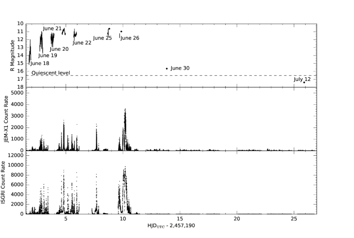
Figure 1: Overall outburst lightcurves based on time-resolved data. Integral data are shown with 8 s (JEM-X) and 64 s (ISGRI) resolution to preserve the extremely transient nature of the detected X-ray activity.

We were fortunate in obtaining overlaps between both McDonald and MDM, and the WHT and MDM, in spite of the serendipitous nature of our observations. We can use these to verify both the relative timing and photometric calibration, and in some cases the reality of unusual features of the lightcurves.

Both Argos and Ultracam are synced to GPS time, and should be reliable to much better than the 1 s time resolution employed in this work. To verify the timing calibration of the MDM data, we cross-correlate overlapping lightcurves against both Argos and Ultracam. On June 19 we find $t_{\rm McD}-t_{\rm MDM}=4.5$ s, with MDM data taken at 6 s time resolution. On June 20 we find $t_{\rm WHT}-t_{\rm MDM}=2.3$ s, with 1 s resolution, and on June 24 we find $t_{\rm WHT}-t_{\rm MDM}=-1.5$ s, with 1 s time resolution but very limited overlapping data. We conclude that timing errors in the MDM data are at most a few seconds. They are certainly smaller than the 8 s time-resolution of the public JEM-X data products, but may lead to small offsets with respect to 1 s JEM-X lightcurves.

We find small differences in the flux calibration between overlapping datasets. This is not surprising as MDM used the $R$ filter ($\lambda_{\rm eff}=6588$ Å) rather than $r^{\prime}$ ($\lambda_{\rm eff}=6290$ Å). We measure $r^{\prime}-R=0.15$ between McDonald and MDM on June 19, and $r^{\prime}-R=0.23$ between WHT and MDM on both June 20 and June 24. We attribute these differences primarily to the difference between $r^{\prime}$ and $R$ filters, and to a lesser extent the crude calibration applied, neglecting colour terms between the target and comparison stars. Where appropriate we convert both McDonald and WHT data to the $R$ band for comparison using the colour terms measured from simultaneous data. For LCO $r$ data we adopt $r-R=0.19$ as the average of McDonald and WHT measurements.

3 Lightcurves

3.1 Overall Morphology and Slow Variations

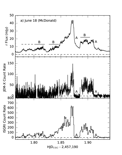
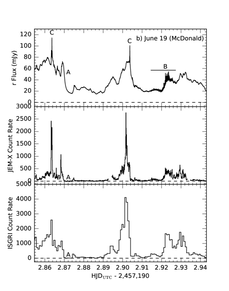
Figure 2: McDonald data compared to Integral data. Labels A denote smooth decays, B indicate periods of rapid optical flaring, and C denotes fast flares at peak light.

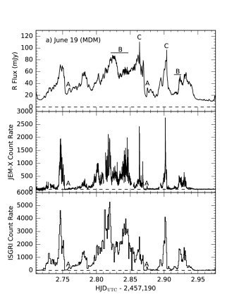
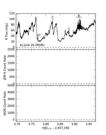
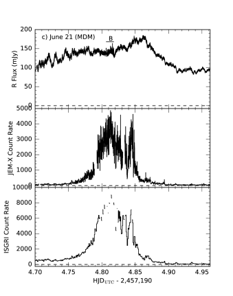
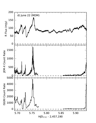
Figure 3: MDM data compared to Integral data. Annotations are the same as in Fig. 2. Where Integral panels are blank, no data were taken at that time.

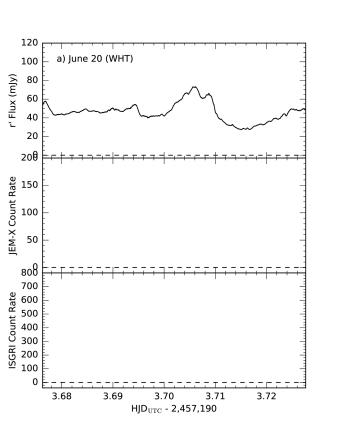
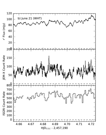
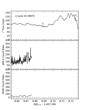
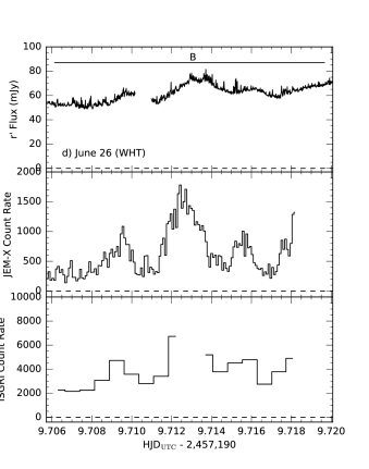
Figure 4: WHT/Ultracam data compared to Integral data. Annotations are the same as in Fig. 2. Where Integral panels are blank, no data were taken at that time.

We compile all the optical lightcurves, transformed to $R$, in Fig. 1, and show individual nights’ lightcurves converted to fluxes in Figs. 2–4. We began our coverage when the source was hitting minimum brightness about a magnitude above quiescence, and followed through the rise to an apparent plateau and then the drop back to quiescence. Our coverage is much less intensively sampled than that of Kimura et al. (2016) which reveals a more complex behaviour. The rising phase involved continual large amplitude variability, with minimum and maximum magnitudes generally rising. Following Gandhi et al. (2016), we refer to all of this heterogeneous behaviour which is ubiquitously present to some degree in most lightcurves on timescales of minutes or longer, as slow variations. At times shorter timescale flares are superposed on the slow variations (Section 3.3). The plateau phase exhibited a generally more stable level interspersed with dips or recurrent oscillations. Shortly after the our last time resolved observation, Kimura et al. (2016) saw the source decline back to fainter levels, as also seen in our LCO data.

Muñoz-Darias et al. (2016) show that H$\alpha$ equivalent widths were below $\sim 300$ Å until June 28, so in all of our time-resolved observations, the $r^{\prime}$ and $R$ band (FWHM$\sim 1400$ Å and 1600 Å respectively; Fukugita, Shimasaku, & Ichikawa, 1995) should be dominated by continuum light. While the line contribution is not negligible, the large amplitude variations seen cannot originate in emission lines alone.

We see dramatic optical variations during the rise. In this period there are multiple occasions when the X-ray flux vanishes (at the limits of Integral sensitivity), and the optical flux is minimized. Generally, a correspondence can be seen between features in X-ray and optical lightcurves, although this is not perfect in detail, and virtually breaks down on June 21. Nonetheless, the similarities between the detailed X-ray and optical lightcurves are more prominent than their differences), and this is most clearly apparent at high energies. The JEM-X lightcurve, which is likely strongly affected by absorption (Motta et al., 2017a; Motta et al., 2017b), is notably more transient than the higher energy ISGRI one, and quite a good correspondence is in fact present between optical and ISGRI lightcurves in Figs. 2–4.

3.2 Smooth Decays

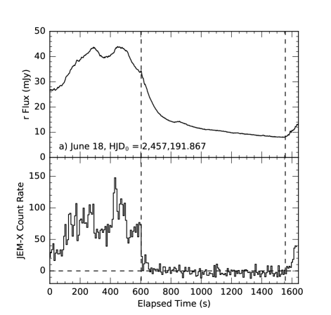
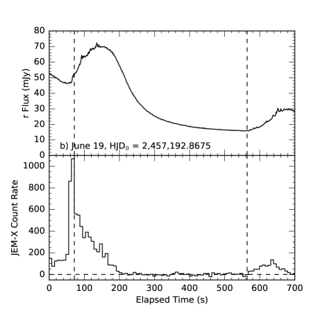
Figure 5: The two most pronounced examples of smooth optical decays after sharp X-ray drops.

On a number of occasions indicated by A in Figs. 2 & 3 we see rather smooth optical decays with a near-exponential form. These can extend over more than a magnitude in brightness and last for $\sim 5-15$ minutes. On every occasion they correspond to dramatic drops in the X-ray and gamma-ray flux to undetectable levels. We show expanded views of the two most pronounced events in Fig. 5. Both are taken from McDonald data, one from June 18 and the other from June 19. On June 18, both X-ray and optical lightcurves are complex, but on June 19, the X-rays are dominated by a single pronounced peak. The optical then peaks 1–2 minutes later. On June 18 we see the decay sustained for 1000 s, and on June 19 for 400 s, both much longer than light travel times could account for. Similar behaviour is seen in multiwavelength observations by Tetarenko et al. (2017) and examined in detail by Dallilar et al. (2017); we will discuss this further in Sections 7.3 and 7.5.

3.3 Optical Flaring Transitions

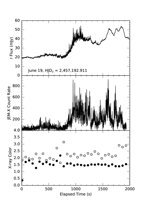
Figure 6: Example of a quick transition in the optical flaring behaviour. seen by McDonald on June 19. The JEM-X 5–25 keV lightcurve at 1 s resolution is plotted for comparison, together with the 64 s binned evolution in X-ray colours as defined in Fig. 10b). White circles are the soft colour ([10–25 keV] / [5–10 keV]), black circles are the hard colour ([60–200 keV] / [25–60 keV]).

Another recurrent characteristic is abrupt changes in the rapid flaring in the lightcurve. Periods of rapid flaring are signified by B in Figs. 2–4, and we expand one of the most dramatic examples in Fig. 6.

When present the flaring can have large amplitude ($\la 0.5$ mag) on timescales of a few seconds. We identify these as periods of repeated flaring on timescales much less than 30 s, with amplitudes much larger than the noise in the data. We attempted to classify them automatically using, for example, the r.m.s. variability within short time bins, but found that the large variety in behaviour produced many false positives. Instead, we selected B regions by eye, using the local r.m.s. variability as a guide. This variability has been examined much more extensively by Gandhi et al. (2016) and Gandhi et al. (2017) who find comparable or larger amplitudes which can be unresolved at a 24 ms time-resolution. The transition between flaring and non-flaring optical emission can emerge in the space of about a minute coincident with no apparent change in X-ray behaviour. In particular, in the example shown in Fig. 6 the 1 s resolution JEM-X lightcurves show that X-ray flaring continues virtually unchanged after the correlated optical flares subside. There is no appreciable change in X-ray colours during the transition; the hard colour is very stable, and the soft colour shows fluctuations probably associated with variable absorption. We will discuss this further in Section 7.4.

3.4 Discrete Optical Flaring Events

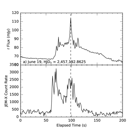
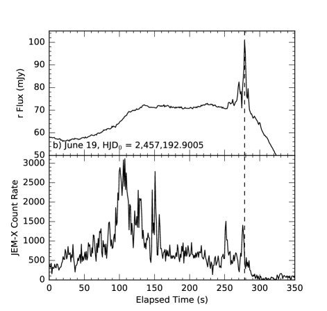
Figure 7: Close-up of the two large amplitude transient optical flaring episodes seen by McDonald on June 19. The JEM-X 5–25 keV lightcurve at 1 s resolution is plotted for comparison.

Even more intriguing are several occasions, marked with C in Figs. 2–4, when short-lived and discrete optical flaring emerges. In two cases seen on June 19, expanded in Fig. 7, these occur close to the peaks of very strong X-ray flares and are strong, peaking at $\sim 40$ percent above the persistent optical flux. These events were both seen independently by McDonald and MDM, so are clearly real. While there is a general association with extremely strong, sharp X-ray flares, as seen in Fig. 2b, in detail the correspondence between X-ray and optical behaviour is poor as shown in Fig. 7. During the first of these two events, the optical peaked about 40 s after the strongest X-ray peak, but did coincide with a second group of blended flares. The second optical event occurred about 170 s after the largest X-ray peak, but may be associated with a smaller X-ray peak a few seconds earlier. If the associations are real rather than chance alignments, then the relative strengths of flares in X-rays and optical are again very weakly coupled, similar to the way in which optical flaring transitions can occur with no apparent change in X-ray behaviour (Section 3.3).

Two other events were observed by MDM (June 20) and Ultracam (June 25) during declines from peaks, and earlier on June 25 transient optical flaring occurs in the middle of a relatively flat, and otherwise unremarkable section of Ultracam lightcurve (see Gandhi et al., 2017, for discussion of this Ultracam event). No Integral data were available for these events, although one was observed by NuSTAR (Gandhi et al., 2017).

The transient flaring properties seem similar to those during the more extended periods described in the previous section, although the first three events are dominated by a single extremely strong optical flare. The proximity with strong X-ray flares in two of the events suggests a connection, even though the largest X-ray and optical flares are not simultaneous. While the last event observed by Ultracam occurred in a relatively flat optical phase, X-ray coverage at the beginning of this lightcurve indicates that X-ray flaring was occurring, and not producing pronounced effects on the optical lightcurve. It therefore remains quite possible that all four events occurred close in time to sharp X-ray flares. Gandhi et al. (2017) suggest that the weak Ultracam event marks a state transition between the quiescent early part of the June 25 observation and the much more active later phase.

4 X-ray and Optical Flux Correlations

We compare inferred X-ray and optical luminosities in Fig. 8. Each point is based on summing average JEM-X and ISGRI fluxes during a 200 s bin, and converting to an (absorbed) isotropic source luminosity for a 2.39 kpc distance. Similarly, the optical flux density during the 200 s bin is converted to an estimate of optical luminosity in $\nu L_{\nu}$ form. X-ray to optical lags of order a minute or less inferred in Section 6 are smaller than the time-bin used here so have negligible effect on the plotted relationships.

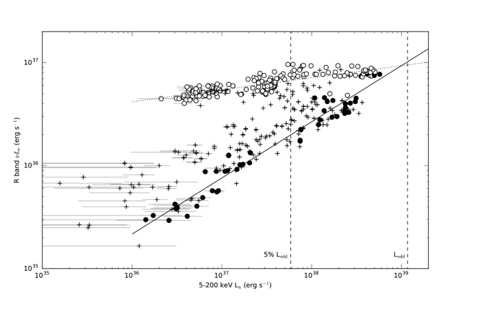
Figure 8: Optical vs. X-ray/gamma-ray luminosity during outburst. Solid circles are times when strong rapid optical flaring was present. These are the periods identified by B in Section 3.3. The solid line, with slope 0.55, is a power-law fit to this subset of data. Open circles are times when little optical variability was present and comprise all of the MDM data from June 21, the second half of the MDM data from June 22, and WHT data from June 25. The dotted line, with slope 0.12, is a power-law fit to this subset of data. The remaining optical data that do not fall clearly into either of these categories are marked with pluses.

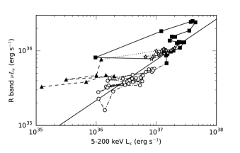
Figure 9: Optical vs. X-ray/gamma-ray luminosity based only on June 18 data from McDonald. Four sections are identified, with times expressed as HJD${}_{\rm UTC}-2,457,190$ as in Fig. 2: before time 1.845 (open circle, dot-dash line), 1.845–1.88 (filled square, solid line), 1.88-1.91 (open star, dotted line), after 1.91 (filled triangle, dashed line).

We see correlations between X-ray and optical fluxes within each observation. Furthermore, several broader patterns across observations emerge. Firstly we note that the lower envelope of all of the observations traces a quite distinct power-law. This is followed over two orders of magnitude in X-ray luminosity. Secondly a distinct set of observations at high optical fluxes appear to trace a flatter line, forming an upper envelope.

We can define these subsets more clearly by examining variability in the optical lightcurves. First we select fluxes corresponding to periods of rapid optical flaring labelled B in Section 3.3. These points, shown with solid circles in Fig. 8 are all clustered along the lower envelope. We fit a power-law to these data points and obtain a power-law index of $0.54\pm 0.02$, i.e. $\nu L_{\nu}(R)\propto L_{\rm X}^{0.54}$. The Pearson linear correlation coefficient between the logarithmic fluxes is 0.97. We test the significance of this correlation using a Monte Carlo permutation test. We preserve ordering within each night’s data to account for strong auto-correlations within the data, but randomly reorder the nights amongst themselves. For reach trial resampling we independently reorder X-ray and optical data in this way, and then also apply a random cyclic shift between the two datasets, and recalculate the correlation coefficient. We finally determine the fraction of these permutations which produce a correlation (or anti-correlation) of magnitude larger than that observed. In this case the fraction of trials with an absolution correlation larger than 0.97 (i.e. the probability of such a strong correlation arising by chance) is $2\times 10^{-4}$, so this relationship appears to be robust.

The clumping around the upper envelope is harder to define within small subsets of data, but seems to be epitomized by MDM data from June 21 (when a large X-ray flare produces no pronounced optical response), from the second half of the MDM data on June 22, and Ultracam data from June 25. We selected these lightcurves by choosing those which show the weakest optical variability, sometimes even when large amplitude X-ray variations occur, as was notably the case on June 21. We highlight data from these three nights with open circles in Fig. 8. A power-law fit to these data points yields a power-law index of $0.12\pm 0.01$ and a Pearson correlation coefficient of 0.80, with about a 4 percent probability of a correlation this strong arising by chance. There definitely appears to be a clumping in the diagram around the upper envelope. The value of the correlation coefficient does, however, leave the possibility that this is not truly tracing a rising trend with increasing X-ray luminosity. Instead it is possible that different observations with different optical brightnesses may happen to align to produce this trend by chance. Nonetheless, it is clear that the periods of weakest optical variability occur near the upper envelope, when the optical to X-ray flux ratio is highest. Finally we note that the only Ultracam observation to show rapid flaring (June 26) is also the only one to lie on the lower envelope rather than the upper one.

The lower envelope we identify is strikingly similar to the $L_{\rm opt}\propto L_{\rm X}^{0.61}$ correlation identified from outburst to quiescence in a number of BHXRTs (Russell et al., 2006), and that specific to V404 Cyg collated by Bernardini et al. (2016): $L_{\rm opt}\propto L_{\rm X}^{0.56}$. As done by Bernardini et al. (2016), we can extrapolate the lower envelope fit to compare to quiescent data from Hynes et al. (2009), after subtracting the orbital-phase modulated companion star flux to leave the residual accretion emission. We do not show this in Fig. 8 to avoid compressing the outburst data, but we do find the extrapolation falls within about a factor of two of the quiescent accretion light.

Kimura et al. (2017) examined X-ray vs. optical correlations during the 2015 December outburst in a similar way, and found power-law indices of 0.25–0.29. These are based on much more limited time coverage than we have used, however, and sample a smaller dynamic range of luminosity. They considered a single relation, rather than looking at envelopes of a more complex behaviour, and found a power-law index intermediate between our two cases. Their results then appear broadly consistent with the range of behaviour we observe.

As the inferred X-ray luminosity increases the two envelopes converge. With a little extrapolation, the power-law fits actually join very close to the Eddington limit ($\sim 0.85L_{\rm Edd}$). Given uncertainties in distance and black hole mass, and the intrinsic geometric uncertainties inherent to applying the Eddington limit to a disc accreting system, this is quite a good agreement. This apparent convergence is borne out by the group of points seen at the highest inferred luminosity where we see both optically flaring (i.e. lower envelope), and low variability (i.e. upper envelope) segments of data coincident in the diagram.

The correlation between X-rays and optical along the envelope is most pronounced when the uncorrelated optical component is minimized on June 18. We expand the correlation for this night in Fig. 9, dividing it loosely into four phases, for which we refer to times $t={\rm HJD}_{\rm UTC}-2,457,190$ corresponding to the time axis in Fig. 2. During the first phase, $t<1.845$, the source lies just above the envelope, and moves up and down roughly parallel to it. The X-rays are continuously present, and both they and the optical emission maintain low level variability. During the major flare of this observation, $1.845<t<1.88$, the fluxes move parallel to the envelope to the highest fluxes reached on this night, before entering an X-ray dip where the X-ray flux dramatically decreases, with optical flux decaying smoothly, and never quite even reaching the level seen at the beginning of the night. This has the effect of moving the source away from the envelope, with the optical appearing independent of the instantaneous X-ray brightness. After the dip, X-rays resume activity during $1.88<t<1.91$, moving the source back to the envelope, overlaying the position occupied earlier in the night. Finally for $t>1.91$, the X-rays enter a more extended dip, allowing the optical to more fully decay back to levels seen at the beginning of the night. At this point, the X-rays are much fainter than initially seen so the source has again moved well away from the envelope. The optical then appears to be sustained at a level unconnected to the X-ray flux. Detailed examination of this observation, then, shows that the envelope is followed within a night, and not just from night to night.

Finally, we note that the two states seen in the X-ray vs. optical relations are quite different to the behaviour of most BHXRTs described by Russell et al. (2006) which are optically fainter in softer states. This behaviour was, however, seen in the 1989 outburst of V404 Cyg, manifesting as high outlier points, and seems to be a characteristic unique to, but repeatable in, this source.

5 Associations Between Optical Variability and X-ray Colours

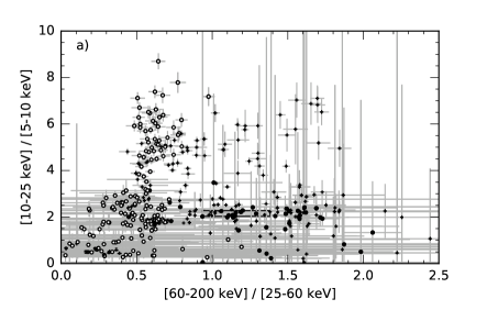
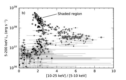
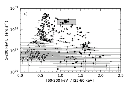
Figure 10: Integral colour-colour and hardness-intensity diagrams at the times overlapping with optical observations. Symbols correspond to those used in Fig. 8, with filled circles indicating bins showing rapid flaring when the source was on the lower-envelope of the X-ray/optical diagram, and open circles indicating the optically bright upper envelope when little optical variability was present. The shaded grey area corresponds to the time when Ultracam saw persistent, intense, rapid flaring (Gandhi et al., 2016). In the panel (b) (the soft hardness-intensity diagram), the shaded area is obscured by a group of points at (2.15, $2.3\times 10^{38}$).

We have identified two distinct subsets of optical–X-ray/gamma-ray behaviour which define boundaries in the flux relationships. The lower-envelope is roughly traced by the $L_{\rm opt}\propto L_{\rm X}^{0.56}$ line and sometimes shows rapid ($<30$ s) optical flaring. The optically bright upper envelope approximately follows $L_{\rm opt}\propto L_{\rm X}^{0.12}$ with the optical weakly variably and almost uncorrelated with X-rays. We can now examine how these relate to X-ray color variations. We show in Fig. 10 colour-colour and hardness-intensity diagrams based on Integral data at the time of optical observations. Note that the bands used (see Section 2.5) are skewed to higher energies than usual colour-colour and hardness-intensity diagrams (e.g. Dunn et al., 2010) due to the sensitivity range of Integral, and have been chosen to highlight the difference between the two categories of optical observations. In particular, we see the most dramatic differences between upper and lower envelope data when considering a hard X-ray (ISGRI) colour.

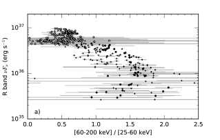
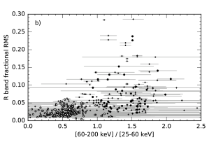
Figure 11: Optical luminosity (upper), and fractional r.m.s. within a 200 s bin (lower) as function of hard X-ray hardness. These quantities are clearly related, with the relation between hard colour and optical luminosity much clearer than that with soft colour. Generally, states with harder X-ray spectral shapes are associated with fainter and more variable optical lightcurves. Symbology is the same as in Fig. 8

We have differentiated a subset of points corresponding to the lower and upper envelope points in the X-ray vs. optical luminosity plot (Fig. 8). The differentiation is seen most clearly in the hardness-intensity diagram using the hard (ISGRI) colour, where we see that the lower-envelope is characterized by a much harder hard colour than the upper envelope, indicating an excess of flux above 60 keV (or a deficit in the 25–60 keV range). This holds across a wide spread of X-ray luminosities, although the two sets of points converge in hard colour as the Eddington limit is approached (as the two envelopes also converge in Fig. 8). We test this differentiation by performing a Kolmogorov-Smirnoff test to check if the distribution of hard colours seen in the lower and upper branches could be consistent with the same distribution. As expected from the colour-colour diagram, this is strongly ruled out with (formally) a $10^{-21}$ probability that they are drawn from the same distribution of X-ray colours.

The softer hardness-intensity diagram (using the JEM-X colour) shows two tracks, diverging from the highest luminosity points. The upper one decreases in apparent luminosity while becoming substantially harder, and probably represents variability induced by changing absorption. No periods of rapid optical flaring appear to be associated with this track. The lower track decreases in apparent luminosities while remaining quite soft in the JEM-X band. These most likely involve real decreases in underlying X-ray luminosity, rather than just changes in line-of-sight absorption. The second track involves both points identified with the upper and lower envelope. These two tracks, then, do not seem associated strictly with the lower and upper envelopes, although the hard upper track does appear to preclude rapid flaring.

Finally, the colour-colour diagram contains elements of both of the other diagrams. The lower-envelope points mainly involve changes in the hard (ISGRI) colour, and upper envelope points mainly track changes in the softer (JEM-X) colour.

We further examine the relationship between hard X-ray colour and optical variability (defined by the r.m.s. variation within a 200 s time bin) more quantitatively in Fig. 11. This shows that times when the hard X-ray spectrum is hardest are associated with lower and more variable optical fluxes. These two relationships hold across the dataset as a whole, and are independent of any classification into lower or upper envelopes. Many of the phases when the ISGRI spectrum is quite hard do not involve rapid optical flaring, so this indicates that these phases must also be associated with the slower timescale optical variations being fainter and more variable as well. The rapid flaring appears to be a symptom of things going on, but is not (alone) responsible for the increased r.m.s. when the hard colour is hardest.

Specifically, we find that the optical fluxes appear to be anti-correlated with ISGRI colour. This does not appear to be a linear correlation, even with respect to logarithmic fluxes, so we test its significance using Spearman’s rank-order correlation. We find a correlation coefficient of -0.75, with a probability of producing a chance correlation this large of about $3\times 10^{-4}$. The optical r.m.s. variability is positively correlated with hard hardness, although the dispersion of the correlation also increases as the ISGRI spectrum gets harder. What does seem to be true is that large values of optical r.m.s. variability are only seen when the hard X-ray spectrum is quite hard. Quantitatively, we find a Spearman rank correlation coefficient of 0.61 between the X-ray colours and optical r.m.s. values, with a probability of chance correlation below $10^{-5}$.

6 X-ray/Optical Lags and Reprocessing

Optical variations generally appear to be lagged and smeared with respect to the X-ray ones. The smearing is ubiquitous, with some exceptions for periods when rapid optical variability emerges, e.g. June 19, and June 26. Lags are sometimes harder to see directly in the lightcurves, as the correspondence in strength of X-ray and optical flares is poor. A lag is most clearly visible on June 26, when in addition to rapid optical flaring, slow variations correlate with X-rays, but are lagged by about a minute.

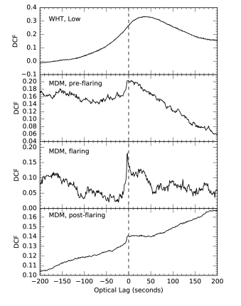
Figure 14: Discrete CCFs through the large flare seen in X-rays on June 21. The top panel uses the whole WHT dataset from that night. The MDM panels correspond to times 4.754–4.795, 4.795–4.820, and 4.820–4.894 respectively.

We quantify X-ray to optical correlations and their lags using cross-correlation functions (CCFs). For this purpose we combine optical lightcurves with JEM-X ones generated at a matching time-resolution. We choose to construct discrete CCFs (DCFs; Gaskell & Peterson, 1987), since overlaps sometimes involve discontinuous segments. We show all available CCFs over a wide-range of lags in Fig. 12. In every case except the MDM lightcurve from June 21 we see CCFs dominated by a single clear peak slightly after zero lag. These are all relatively broad, although vary substantially in width, and peak at lags of 10–50 s. This overlaps the 22.5 s and 34.8 s lags reported in the 2015 December outburst (Kimura et al., 2017, 2018). On June 21, the very large X-ray flare which is relatively uncorrelated with optical behaviour on long timescales dominates the MDM CCF producing a general rise towards late times. Close examination shows a small peak superposed on this rise close to zero lag (see Fig. 14 and discussion below).

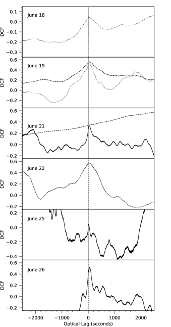
Figure 12: Discrete CCFs. McDonald data are shown dotted, MDM data dashed and WHT data in solid lines.

Other studies (e.g. Rodriguez et al., 2015) have claimed that quasi-correlated optical flaring was also seen with the optical lagging the X-rays by anywhere from $<1$ min to 20–30 min, varying from flare to flare. The latter observation is quite inconsistent with our finding that the dominant X-ray/optical CCF peaks are usually quite close to zero lag. As noted earlier, however, the lightcurves are complex and sometimes show strong optical counterparts to weak X-ray flares and vice-versa. This would be missed with poorly sampled data, leading instead to matching the nearest bright flare and inferring a larger lag than is real. Our higher time resolution optical coverage breaks these degeneracies.

In considering a dataset as rich and inhomogeneous as this it is helpful to divide the data into sub-samples based on behaviour. One important sub-sample comprises segments of lightcurves when rapid optical flaring is occurring. The best for this purpose are June 19 (McDonald night 2), and June 26 (Ultracam night 5), as both provided 1 s time resolution optical lightcurves spanning relatively extended periods of flaring. On June 19, we also have data for a second earlier period of rapid flaring, albeit at lower time-resolution, from MDM night 1. We show the June 19 CCFs in Fig. 13a and b, and the June 26 CCF in Fig. 13c. The width of a peak in the cross-correlation function indicates the timescales of correlated variability. A narrow peak is only possible if both the X-ray and optical variability are dominated by short timescales; a slow variation in one or both lightcurves will smear the correlation over a larger range of lags leading to a broader peak. We then expect that correlations involving the rapid optical flaring will be narrow and those involving the slower variations will be broad. The MDM data show that the rapid flaring is the dominant correlation during the first period of flaring on June 19, providing a narrow peak near zero lag. This is consistent with Ultracam flaring studies which suggest a $\sim 0.1$ s lag (Gandhi et al., 2016, 2017). The rapid response associated with fast flaring has now been seen in a number of other BHXRTs as summarized in Section 1. During the second flaring period on June 19, we clearly also see a sharp peak near zero lag, but it is superposed on a lagged and smeared response. On June 26, the CCF is dominated by the slow variations, but a small sharp peak can also be seen close to zero lag. In these latter two cases, then both rapid flaring and slow variations are present, correlated with the X-rays, and seen in the CCF.

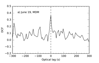
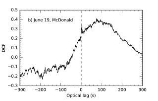
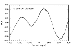
Figure 13: Optical vs. X-ray cross-correlation functions during the rapid flaring episodes on June 19 and 26. Panel (a) is taken from MDM data at 6 s time resolution, towards the end of the first episode labelled B in Fig. 3a, times labelled 2.83720–2.84748. Panel (b) is taken from McDonald data at 1 s time resolution, during the second episode labelled B in Fig. 3a (the only B episode in Fig. 2b; times labelled 2.921–2.926). Panel (c) uses the whole Ultracam dataset from June 26. While a sharp and near instantaneous response is seen alone during the first episode, during the second we clearly also see a broad, lagged response, which appears quite distinct from the peak at zero lag. The June 26 data look similar to the panel (b), but which the sharper peak at zero lag being weaker relative to the large amplitude slow variations.

We also examine the evolution of the CCF through the large X-ray flare seen on June 21 in Fig. 14. For this night, we have WHT/Ultracam data from the beginning of the night, followed by MDM data for the remainder. While the X-ray flare exhibits the largest X-ray flux seen in our simultaneous dataset, and a dynamic range of about a factor of fifty, the optical data only vary by a factor of two, and do not obviously correlate with the X-ray flare. A correlation on shorter timescales is clearly seen in the Ultracam lightcurves (Fig. 4b) and is reflected by a pronounced CCF peak (Fig. 14), but the MDM CCF appears dominated by a general rise which is likely due to uncorrelated variability. On closer examination a peak can be seen close to zero lag; the evolution of this peak is shown in Fig. 14. Combining these four snapshots of the CCF evolution, we see that the CCF is quite broad and strongly lagged ($\sim 35$ s) before the flare, similar to the lagged and smeared response seen at other times. During the flare rise, the peak moves to shorter lags ($\sim 10$ s) and the response becomes narrower, although with an asymmetric tail to longer lags. Near the peak of the flare a short episode of rapid flaring occurs (labeled B in Fig. 3c), during which a very narrow peak occurs, similar to those discussed above for June 19 and 26, before the CCF reverts to the short peak delay, extended tail form for the decline from the flare.

7 Discussion

7.1 Binary geometry and lag expectations

Recurrent X-ray/optical correlations indicate that the optical emission is causally linked in some way to the central engine around the black hole, either because one is driving the other, or because they share a common cause. They could arise from the same region, for example the base of the jet, or from different regions coupled by irradiation or plasmon ejection. To understand optical variations, then, we need to understand the binary geometry and the mechanism(s) coupling X-ray variations to the optical. We have seen that a lag of about a minute is common in slower timescale variability, and that this is accompanied by comparable smearing of the signal. An independent analysis by Alfonso-Garzón et al. (2018) of individual flares also identified a class of optical flares lagging the X-rays by $<2$ min). This lagged, smeared correlation could naturally arise either from light travel timescales within the binary if the optical is produced by reprocessing of high energy irradiation (O’Brien et al., 2002), or from expanding plasmons in the jet becoming optically thin at progressively longer wavelengths with time (van der Laan, 1966).

Light travel timescales are straightforward to calculate given estimates for binary parameters. For V404 Cyg, assuming orbital period $P=6.47$ days, mass ratio $q=0.06$, and black hole mass $M_{1}=9.0$ M_⊙ (Khargharia, Froning, & Robinson, 2010), the binary separation is about $2.2\times 10^{12}$ cm. Assuming the disc is limited to 90 percent of the Roche lobe radius, the maximum disc radius is about $1.2\times 10^{12}$ cm. Light travel time delays from the disc should then range from 0–80 s, with the response weighted towards shorter lags within the range (O’Brien et al., 2002). Similar estimates were made independently by Alfonso-Garzón et al. (2018).

Wavelength dependent lags due to expanding plasmons are harder to estimate reliably, depending on plasmon properties. Rodriguez et al. (2015) suggested optical lags should be $\ga 10$ min, but this is presumably based on analogy with other sources. In the specific case of V404 Cyg, we can find ground truth in the sub-mm to radio range where signatures of this behaviour are clearly seen with frequency-dependent lags consistent with a plasmon model (Tetarenko et al., 2017). This model predicted that the radio emission lagged the actual ejection events by tens of minutes. In the model, the frequency dependent lags, given by their equation 15, scale approximately as $\nu^{-0.33}$ to $\nu^{-0.5}$ with different indices corresponding to the range of electron energy distributions inferred across a range of flares. We can use this lag prescription from Tetarenko et al. (2017) together with their tabulated parameters for the eight ejections identified to extrapolate the range of lags expected in the $r$ or $R$ band. The expected lags range from 20–110 s, shorter than expected by Rodriguez et al. (2015).

7.2 Rapid variability and the central engine geometry

The timescale of rapid optical flaring (during periods labelled B in the lightcurves) is much less than the light-travel timescale across the disc estimated above, so this behaviour cannot arise in reprocessing. At the same, time, the flaring does at times clearly correlate with that seen by JEM-X (see Section 6), so neither can this arise from local variability (e.g. due to magnetic reconnection; Zweibel & Yamada 2009) in the outer disc. It is most likely then that this rapid optical flaring originates close to the central engine producing X-rays. It probably arises in direct jet emission, although the timescale is much shorter than that estimated above for plasmon ejection (Gandhi et al., 2016, 2017), suggesting a different variability mechanism. Direct optical emission from the corona has also been proposed by Dallilar et al. (2017).Alfonso-Garzón et al. (2018) considered similar possibilities for flares with no optical lag.

Based on NuSTAR, Swift, and INTEGRAL observations an X-ray picture of the central source geometry has emerged, although many features remain in question. The X-ray spectrum is dominated by power-law components, presumably associated with inverse Compton scattering in hot coronal material or the base of the jet, with superposed Compton reflection (Walton et al., 2017). A disc black body component may have also been present at the lowest energies, although Motta et al. (2017b) could not confirm this with Swift. The coronal X-ray source illuminating this putative inner disc is required to be compact, with height less than ten gravitational radii. Strong and variable absorption occurred ubiquitously (see Section 7.4). Sánchez-Fernández et al. (2017) identify the source as predominantly being in the canonical hard state (Remillard & McClintock, 2006), which is usually associated with a recessed disc. These hard state periods coincide with hard ISGRI colours. Periods of softer ISGRI colours are identified as transitions into intermediate or ultra-luminous states by Sánchez-Fernández et al. (2017) and could then be associated with the disc moving inwards. Walton et al. (2017) argue that X-ray flares are likely also associated with transient jet ejections. Synthesizing these results, a possible scenario is then that the disc is recessed between large flares, with a quasi-steady compact jet. Transient instabilities in the jet could give rise to rapid optical flaring (Malzac et al., 2018). During major flares, the disc moves inward with the flare then ending with disruption of this transient disc and ejection of a plasmon, leading to a delayed optical flare (Mirabel et al., 1998). Irradiation of the outer disc during flares is also possible, although may be inhibited by the large amounts of local absorption, discussed in section 7.4. We will focus more on the roles of plasmon ejection and irradiation in mediating slow variability in Section 7.3, and for the remainder of this Section will focus on the fastest optical variability.

This rapid optical flaring, sometimes on sub-second timescales, is notably redder than the slower variations consistent with an origin in synchrotron emission from the base of the jet (Gandhi et al., 2016, 2017). Between our June 18 and June 19 McDonald observations, when several of these rapid flaring episodes occurred, Trushkin, Nizhelskij, & Tybulev (2015) reported a radio detection with an inverted spectrum, suggesting optically thick emission from a compact jet, adding support to the idea that jet activity was present at this time. Based on an 0.1 s delay between X-ray and rapid optical flares, the optical emission region producing these rapid variations is inferred to lie $\la 0.1$ light seconds (about 1000 Schwarzschild radii) above the black hole, and so is part of the central engine region.

We find that this rapid optical flaring is associated with the lower-envelope in the X-ray/optical flux relationship (Section 4). Times when rapid flaring are present are associated with times when the hard X-ray colour (the ISGRI colour) is quite hard (Section 5). As noted above, hard ISGRI colours are identified by Sánchez-Fernández et al. (2017) with the canonical hard state. Our lower envelope then appears to correspond to this hard state, as do rapid optical flares. This is consistent with behaviour in other BHXRTs.

The rapid optical flares themselves can quite suddenly appear and disappear with no change in X-ray intensity or colour (e.g. Fig. 6) and they do not appear to be immediate consequences of changes in the X-ray state. These changes in optical flaring may represent variations within the jet itself downstream from where X-rays are produced, such that sometimes intense optical variability is seen and sometimes it is not. One proposed mechanism for this rapid variability is internal shocks within the jet caused by fluctuations in the jet velocity (Malzac et al., 2018).

7.3 Are slow variations driven by plasmon ejections or disc irradiation?

Rapid optical variability in V404 Cyg (second-timescale and faster) is clearly associated with the central engine and jet, as discussed above. This rapid flaring is confined to the lower envelope of the X-ray vs. optical relationship, but except for the peaks of extremely transient flaring, it never dominates the optical flux. It remains to elucidate then whether this correlation itself reflects jet behaviour, with the slower optical variations that dominate it arising in expanding plasmons downstream of the jet base, or whether the correlation instead reflects irradiation of a disc or wind component. Both effects are expected to be present at some level, and both produce a correlation comparable to $F_{\rm opt}\propto F_{\rm X}^{0.6}$ (Russell et al., 2006), and so jet and disc may both be contributing to the behaviour.

As noted in Section 7.1, radio and sub-mm observations indicate that larger scale plasmon ejections did occur at other times in this outburst. In particular, Miller-Jones et al. (2019) actually resolve radio ejections on several occasions, with most intensive coverage on 2015 June 22 (MJD 57,195. Tetarenko et al. (2017) show multi-frequency lightcurves with simultaneous X-ray and optical coverage through a series of flares also on June 22, beginning with the large flare caught at the end of the fourth night of our MDM data. Three X-ray flares are covered, two large and one small. The ends of the two large ones both show an optical decay similar to our exponential decays, and both are followed by flares at sub-mm, then mm, then radio frequencies. A model of expanding plasmons (van der Laan, 1966) provides remarkable agreement with the multi-frequency lightcurves and the set of flares observed can be well modelled by assuming a series of eight ejection events, with the X-ray cut-off and optical decay corresponding to two of the events.

The optical behaviours we saw on June 19, and that reported on June 22 by Tetarenko et al. (2017), both resemble that seen in GRS 1915+105, where a disappearance of X-ray flux is also followed by an infrared, and then a radio flare (Mirabel et al., 1998). Those events were interpreted as due to disruption of the inner disc and ejection of an expanding plasmon, which then emits at progressively longer wavelengths as described above. We see optical lags of order a minute in V404 Cyg, in contrast to the 15 minute IR lag seen in GRS 1915+105 (c.f. Rodriguez et al., 2015; Alfonso-Garzón et al., 2018, for claimed longer lags). As estimated above, however our shorter optical lag, around one minute, is expected from the ejection model of Tetarenko et al. (2017) based on the flares they observe in V404 Cyg. A one minute lag would also be consistent with light travel timescales across the disc, so it remains possible that either the slow optical variations arise from direct emission from the plasmons, or from irradiation of the disc or wind by the X-ray flares, or by a combination of both mechanisms. Dallilar et al. (2017) have instead argued that decay events similar to those shown in Section 3.2 occur in stationary material in the corona or base of the jet with the optical decay reflecting synchrotron cooling with no change in magnetic field, rather than the expansion of ejecta.

While the overall lag may be comparable between different models, the wavelength dependence of the lag may differ as plasmon models predict a strong frequency dependence. The high time-resolution multicolour observations of Gandhi et al. (2016) show lags between optical bands, $\sim 4$ s. This is in reasonable agreement with the $\la 10$ s inter-band lags that would be expected based on the Tetarenko et al. (2017) ejection model (Section 7.1.), but does not rule out irradiation which also predicts shorter lags at shorter wavelengths.

Optical colour variations during flares can also be helpful to disentangle variability mechanisms. Gandhi et al. (2016) find that rapid flaring is quite red, as expected for optically thin synchrotron emission, while the slower variations are bluer. The latter could be consistent with either disc reprocessing or self-absorbed synchrotron. Tachibana et al. (2017) argued that the slowly variable component could be further decomposed into a ‘highly-variable component’ with blue colours and flux rising with frequency, and a redder ‘little variable component’ with approximately flat colours invoking both jet and disc emission to explain the components. Kimura et al. (2016) argue based on the spectral energy distribution that the primary optical response to X-rays is mediated by reprocessing while Maitra et al. (2017) suggest that the stability of the colours through large flux changes is inconsistent with irradiation which should become bluer as it brightens.

If large optical flares do arise in the jet, then we would also expect to see polarization signatures. While an optically thick jet would be free of polarization, by its nature the expanding plasmon model produces flare peaks when the plasmon transitions from optically thick to thin at the observed wavelengths, so polarization should be seen at least during the decay of flares when emission is optically thin. Infrared polarization has now been detected from several quiescent, outbursting, and persistently accreting black hole binaries, lending credence to this expectation (Russell & Fender, 2008; Russell & Shahbaz, 2014; Russell et al., 2016; Chaty, Dubus, & Raichoor, 2011). Unfortunately, here too the observational evidence is equivocal with some studies finding variable polarization, and others not, and characteristics that may be more consistent with scattering in a disc outflow rather than from jet synchrotron emission (Tanaka et al., 2016; Lipunov et al., 2016; Shahbaz et al., 2016; Itoh et al., 2017; Kosenkov et al., 2017).

In summary, both jet emission, and X-ray irradiation remain plausible mechanisms to couple the slow variations in the optical, with evidence in favour of both interpretations from colour changes, inter-band lags, and polarization. It is possible that both mechanisms do play a role, and that the inconsistent and equivocal evidence discriminating them is a consequence of this Alfonso-Garzón et al. (c.f. 2018). The apparent bimodal behaviour seen in Fig. 8 also suggests two distinct modes of coupling the X-ray to the optical, with the lower envelope showing characteristics typical of optical jet emission such as the $F_{\nu}\propto\nu^{0.6}$ dependence, rapid optical flaring and the association with hard X-ray colour. More speculatively, the upper branch might represent a disc dominated mode with the optical coupled to X-rays at least partly through irradiation.

7.4 Local absorption

There is considerable evidence for large intrinsic absorption from the inner accretion disc (Motta et al., 2017a; Sánchez-Fernández et al., 2017). The soft hardness-intensity diagram we show in Fig. 10b also shows behaviour suggesting variable X-ray absorption with a track where the source fades and becomes harder. Only a subset of data follow this track, however, and another group of points suggest softening as the source fades. Absorption then may account for some of the variability we see, but not all of it.

Absorbing material may impact not only our view of X-rays, but also the ability of X-rays to irradiate the outer disc and wind. It also means that the X-ray lightcurve we see may not be the same as the outer disc sees. This could partially explain the inconsistencies that we see between X-ray and optical flare amplitudes. Motta et al. (2017b) suggest that X-ray behaviour implies two layers of absorption: a high column density inhomogeneous region within 100 gravitational radii, and a more diffuse and homogeneous one at larger radii. The inhomogeneous absorption then occurs inside the optically dominant part of the disc. Strong optical flares with weak X-ray counterparts could arise if the X-ray emission is obscured but optical emission is visible. Absorption will affect high energy photons least, so the ISGRI lightcurve, which usually does resemble the optical one more closely than the JEM-X lightcurve does, should better trace the central activity. In an irradiation model the optically emitting regions of the disc will be directly visible, and are likely to be illuminated by many lines of sight at different azimuths, so they will not see the same localized absorption as we see in X-rays. In a jet model, optical synchrotron flares associated with transient jets are expected to be emitted from beyond $\sim 1000$ Schwarzschild radii above the black hole (Gandhi et al., 2017). The inner absorption region inferred by Motta et al. (2017b)is then likely too small to obscure the jet base, and the outer region too diffuse and homogeneous.

Obscuration of direct X-ray emission does not explain cases like Fig. 7 where several X-ray flares are seen, with only the last clearly echoed in the optical; it is hard to obscure only the optical emission. If the optical emission is associated with irradiation, there could be a low-altitude obscuring torus that can completely impede irradiation of the outer disc, while we can see over it. Only when this torus mostly dissipates (possibly at the end of a series of flares as in Fig. 7), is the optical disc exposed to irradiation. This kind of behaviour may also explain the cases identified by Alfonso-Garzón et al. (2018) where large optical lags are seen.

7.5 Winds

Optical spectroscopic monitoring revealed a strong, high velocity, but low-excitation wind from the outer disc which appeared to carry away most of the pre-outburst disc mass and terminate the outburst around the time of our last time-resolved observations (Muñoz-Darias et al., 2016; Rahoui et al., 2017). The strong wind from the outer disc inferred by Muñoz-Darias et al. (2016) will have a profound impact on the kind of observations we are making. We can place a lower limit on the density of such a wind quite readily. Muñoz-Darias et al. (2016) estimate that a total mass of at least $10^{-8}{\rm M}_{\odot}$ is expelled over $\sim 10$ days of outburst, implying an average mass loss rate $\ga 2\times 10^{19}{\rm g}{\rm s}^{-1}$. If this emerges uniformly over the whole disc (radius $1.2\times 10^{12}{\rm cm}$) at $0.01{\rm c}$, then the density of the wind should be $\sim 1.5\times 10^{-14}{\rm gcm}^{-3}$, corresponding to a particle density of $9\times 10^{9}$ cm^-3 for pure hydrogen, comparable to density estimates made by King et al. (2015) based on X-ray line emission measures. Finally, if the central source is viewed near edge-on through this wind (as is the case in irradiating the outer disc), then we expect a column of $0.02{\rm gcm}^{-2}$, or $N_{\rm H}\sim 1\times 10^{22}{\rm cm}^{-2}$, again comparable to X-ray based estimates given by King et al. (2015). The uncertainties in this estimate: adopting the minimum mass loss suggested by Muñoz-Darias et al. (2016), assuming the whole area of the disc participates in the wind and using the terminal velocity of an accelerating wind all tend to lower the inferred column density, so this can be considered a lower limit on the mean column. If the mass loss is episodic, as is likely given the extremely variable irradiation of the disc, then at times it will be lower, but at other times it may be much higher. This minimum mean column is about twice the interstellar column. It will produce an enhanced absorption in spectroscopy, but should not completely block our view of the central source and neither will it prevent irradiation of the outer disc, unless the column is episodically or locally much higher.

If large optical variations do arise from reprocessing then the presence of such a strong wind as is inferred will modify both the irradiation itself, and the geometry of the reprocessing material. Signatures of irradiation may then be quite different to those in more normal LMXBs. One effect that can be expected from such a wind is that soft X-rays will only penetrate partially into the wind, leaving the outer region relatively shielded from ionizing radiation. With this picture, such soft X-rays as are present in an already hard spectrum will be absorbed by the wind, leaving only the harder X-rays to irradiate the outer disc. These will penetrate deep into the photosphere, leading to quite long reprocessing times (Cominsky, London, & Klein, 1987; McGowan et al., 2003) which may substantially enhance the observed lags compared to light travel times alone. We then expect that the disc reprocessing signal will be lagged by a combination of light-travel times ($\la 80{\rm s}$), and significant reprocessing times. Observing lags longer than possible from geometrical light travel times alone is then not a problem for the reprocessing model, and these prolonged reprocessing times could contribute to the extended tails to smooth decays described in Section 3.2. In this respect we disagree from Alfonso-Garzón et al. (2018) who only consider geometrical light travel time delays for reprocessing.

8 Conclusions

We have performed a serendipitous campaign monitoring the relationship between optical and X-ray variability in V404 Cyg during the rise and peak of the outburst of 2015 June. We focus on variability on timescales of seconds and longer, finding large amplitude optical variability, usually related to X-ray behaviour, although not perfectly correlated.

We find a relationship between X-ray and optical fluxes bounded by lower and upper envelopes. These envelopes converge around the Eddington limit. The lower envelope is traced by a power-law relation $L_{\rm opt}\propto L_{\rm X}^{0.54}$. At times we see motion along this line within a night, reinforcing its significance as a boundary on the source behaviour. This lower envelope is consistent in power-law index with X-ray/optical relations identified previously by other authors and can approximately be extrapolated all the way to quiescent fluxes. We find a correlation between the position in the X-ray/optical diagram and the X-ray spectrum, with locations close to the lower-envelope corresponding to harder hard X-ray colours ([60–200 keV] / [25–60 keV]). These hard X-ray hard states are identified by Sánchez-Fernández et al. (2017) as the canonical hard state. A subset of data seem to lie above this relationship and distinct from it, defining a an upper envelope approximately tracing a $L_{\rm opt}\propto L_{\rm X}^{0.12}$ relation. These periods are identified by Sánchez-Fernández et al. (2017) as likely corresponding to intermediate and ultra-luminous states in other sources. As well as the X-ray/optical flux correlation, we find the hard X-ray hardness is anti-correlated with the optical brightness and positively correlated with R.M.S. optical variability. It is likely that all of these properties (X-ray and optical flux, hard X-ray colour, and optical rapid variability) are driven by changes in the central accretion rate and geometry. Such changes will directly affect the X-ray spectrum, and optical emission from the jet. They may also affect the efficiency with which the disc can reprocess X-rays, and so affect the slowly varying component of optical emission as well.

The optical variability is quite diverse, but can broadly be divided into two types. Contributing most of the variability are large amplitude, slow variations that probably arise either in X-ray irradiation of the outer disc and its wind, or from expanding jet ejecta, or both. In this respect, our conclusions agree with the recent work of Alfonso-Garzón et al. (2018) which was based on quite different analysis focused on identifying and classifying individual flaring events. These slow variations generally follow X-ray, and especially hard X-ray, behaviour, with a lag and smearing on $\sim$minute timescales. The connection between X-ray and optical is complex, with at times a strong optical response to a weak X-ray flare or vice versa. In part, this is probably due to variable obscuration of the central X-ray source either from our perspective or from that of the outer disc. During extended X-ray quiet periods we see a prolonged tail to this slow response that is seen to continue to fade for up to 1000 s. This is much longer than light travel times in the binary, so if they arise from reprocessing then they require quite a large diffusive reprocessing time to release the energy absorbed from irradiation. The other, and apparently distinct, component of variability is transient rapid flaring showing small or no lag with respect to X-rays. These flares occur simultaneously with the slower, lagged variations and both can then be seen simultaneously in cross correlation functions. The rapid flares appear to be direct synchrotron emission from a standing shock at the base of the jet (Gandhi et al., 2017). These only occur near the lower envelope of the X-ray/optical flux relationship and appear analogous to rapid optical flaring observed in other hard state sources as summarized in Section 1. Sometimes these periods are very short-lived, with a single very large flare. At other times the optical flaring can last for periods $\sim 10$ minutes, then fade away with no apparent change in X-ray colours or variability. Since the rapid optical flaring appears to be associated with the central source itself, this may indicate intrinsic changes in optical production from the base of the jet, rather than effects of absorption.

The 2015 activity of V404 Cyg has provided a fascinating, if short, view of accretion onto BHXRTs. In some respects, including the X-ray state evolution and presence of rapid optical synchrotron flaring it follows patterns identified in other sources. The large orbital period of the system means that the accretion disc is larger than in almost other systems, except for GRS 1915+105 which has its own peculiarities, and this may be responsible for the unusual outburst evolution and strong mass loss which played a large role in the outburst. The impact of outflows on our observations is magnified by a relatively high inclination which ensured our view of the central source was heavily impacted by absorption or complete obscuration by material above the disc. It appears, then, that while the outburst showed many unusual and unprecedented features, these owe more to the large scale environment and viewing angle than to the behaviour of the central source itself.

References

- Alfonso-Garzón et al. (2018) Alfonso-Garzón J., et al., 2018, A&A, 620, A110
- Barthelmy et al. (2015) Barthelmy, S. D., D’Ai, A., D’Avanzo, P., Krimm, H. A. Lien, A. Y., Marshall, F. E. Maselli, A., & Siegel, M. H., 2015, GCN, 17929
- Barentsen et al. (2014) Barentsen G., et al., 2014, MNRAS, 444, 3230
- Bernardini & Cackett (2014) Bernardini F., Cackett E. M., 2014, MNRAS, 439, 2771
- Bernardini et al. (2016) Bernardini, F., Russell, D. M. , Koljonen, K. , Stella, L., Hynes, R. I. , & Corbel, S., 2016, MNRAS, 826,149
- Bradley et al. (2007) Bradley C. K., Hynes R. I., Kong A. K. H., Haswell C. A., Casares J., Gallo E., 2007, ApJ, 667, 427
- Brown et al. (2013) Brown T. M., et al., 2013, PASP, 125, 1031
- Casares, Charles, & Naylor (1992) Casares J., Charles P. A., Naylor T., 1992, Natur, 355, 614
- Casares et al. (1993) Casares J., Charles P. A., Naylor T., Pavlenko E. P., 1993, MNRAS, 265, 834
- Chaty, Dubus, & Raichoor (2011) Chaty S., Dubus G., Raichoor A., 2011, A&A, 529, A3
- Chen, Shrader, & Livio (1997) Chen W., Shrader C. R., Livio M., 1997, ApJ, 491, 312
- Cominsky, London, & Klein (1987) Cominsky L. R., London R. A., Klein R. I., 1987, ApJ, 315, 162
- Corbel et al. (2003) Corbel S., Nowak M. A., Fender R. P., Tzioumis A. K., Markoff S., 2003, A&A, 400, 1007
- Dallilar et al. (2017) Dallilar Y., et al., 2017, Sci, 358, 1299
- Drew et al. (2005) Drew J. E., et al., 2005, MNRAS, 362, 753
- Dunn et al. (2010) Dunn R. J. H., Fender R. P., Körding E. G., Belloni T., Cabanac C., 2010, MNRAS, 403, 61
- Durant et al. (2008) Durant M., Gandhi P., Shahbaz T., Fabian A. P., Miller J., Dhillon V. S., Marsh T. R., 2008, ApJ, 682, L45
- Durant et al. (2009) Durant M., Gandhi P., Shahbaz T., Peralta H. H., Dhillon V. S., 2009, MNRAS, 392, 309
- Durant et al. (2011) Durant M., et al., 2011, MNRAS, 410, 2329
- Fukugita, Shimasaku, & Ichikawa (1995) Fukugita M., Shimasaku K., Ichikawa T., 1995, PASP, 107, 945
- Gallo, Fender, & Pooley (2003) Gallo E., Fender R. P., Pooley G. G., 2003, MNRAS, 344, 60
- Gandhi et al. (2008) Gandhi P., et al., 2008, MNRAS, 390, L29
- Gandhi et al. (2010) Gandhi P., et al., 2010, MNRAS, 407, 2166
- Gandhi et al. (2015a) Gandhi P., Littlefair S., Hardy L., Dhillon V., Marsh T. R., Shaw A. W., 2015, ATel, 7686
- Gandhi et al. (2015b) Gandhi P., et al., 2015, ATel, 7727
- Gandhi et al. (2016) Gandhi P., et al., 2016, MNRAS, 459, 554
- Gandhi et al. (2017) Gandhi P., et al., 2017, Nature Astronomy, 1, 859
- Gaskell & Peterson (1987) Gaskell C. M., Peterson B. M., 1987, ApJS, 65, 1
- Golenetskii et al. (2015) Golenetskii, S., et al., 2015, GCN, 17938
- Homan et al. (2005) Homan J., Buxton M., Markoff S., Bailyn C. D., Nespoli E., Belloni T., 2005, ApJ, 624, 295
- Hynes, Robinson, & Morales (2015a) Hynes R. I., Robinson E. L., Morales J., 2015a, ATel, 7677
- Hynes, Robinson, & Morales (2015b) Hynes R. I., Robinson E. L., Morales J., 2015b, ATel, 7710
- Hynes et al. (2003) Hynes R. I., et al., 2003, MNRAS, 345, 292
- Hynes et al. (2004) Hynes R. I., et al., 2004, ApJ, 611, L125
- Hynes et al. (2006) Hynes R. I., et al., 2006, ApJ, 651, 401
- Hynes et al. (2009) Hynes R. I., O’Brien K., Mullally F., Ashcraft T., 2009, MNRAS, 399, 281
- Hynes et al. (2009b) Hynes R. I., Bradley C. K., Rupen M., Gallo E., Fender R. P., Casares J., Zurita C., 2009, MNRAS, 399, 2239
- Itoh et al. (2017) Itoh R., et al., 2017, PASJ, 69, 25
- Jenke et al. (2016) Jenke P. A., et al., 2016, ApJ, 826, 37
- Jordi, Grebel, & Ammon (2006) Jordi K., Grebel E. K., Ammon K., 2006, A&A, 460, 339
- Jourdain, Roques, & Rodi (2017) Jourdain E., Roques J.-P., Rodi J., 2017, ApJ, 834, 130
- Kanbach et al. (2001) Kanbach G., Straubmeier C., Spruit H. C., Belloni T., 2001, Natur, 414, 180
- Khargharia, Froning, & Robinson (2010) Khargharia J., Froning C. S., Robinson E. L., 2010, ApJ, 716, 1105
- Kimura et al. (2016) Kimura M., et al., 2016, Nature, 529, 54
- Kimura et al. (2017) Kimura M., et al., 2017, MNRAS, 471, 373
- Kimura et al. (2018) Kimura M., et al., 2018, MNRAS, 475, 3083
- King et al. (2015) King A. L., Miller J. M., Raymond J., Reynolds M. T., Morningstar W., 2015, ApJ, 813, L37
- King, Kolb, & Burderi (1996) King A. R., Kolb U., Burderi L., 1996, ApJ, 464, L127
- King et al. (1997) King A. R., Frank J., Kolb U., Ritter H., 1997, ApJ, 484, 844
- King, Kolb, & Szuszkiewicz (1997) King A. R., Kolb U., Szuszkiewicz E., 1997, ApJ, 488, 89
- Kosenkov et al. (2017) Kosenkov I. A., Berdyugin A. V., Piirola V., Tsygankov S. S., Pallé E., Miles-Páez P. A., Poutanen J., 2017, MNRAS, 468, 4362
- Kuulkers (2015) Kuulkers E., 2015, ATel, 7758
- Lipunov et al. (2016) Lipunov V. M., et al., 2016, ApJ, 833, 198
- Loh et al. (2016) Loh A., et al., 2016, MNRAS, 462, L111
- Maitra et al. (2017) Maitra, D., Scarpaci, J. F., Grinberg, V., Reynolds, M. T., Markoff, S., Maccarone, T. J., Hynes, R. I., ApJ, 851, 148
- Makino (1989) Makino F., 1989, IAUC, 4782, 1
- McClintock & Remillard (2006) McClintock J. E., Remillard R. A., 2006, in Compact stellar X-ray sources. Eds. Walter Lewin & Michiel van der Klis. Cambridge Astrophysics Series, No. 39. Cambridge, UK: Cambridge University Press, p157 - 213
- McGowan et al. (2003) McGowan K. E., Charles P. A., O’Donoghue D., Smale A. P., 2003, MNRAS, 345, 1039
- Malzac et al. (2018) Malzac J., et al., 2018, MNRAS, 480, 2054
- Miller-Jones et al. (2009) Miller-Jones J. C. A., Jonker P. G., Dhawan V., Brisken W., Rupen M. P., Nelemans G., Gallo E., 2009, ApJ, 706, L230
- Miller-Jones et al. (2019) Miller-Jones J. C. A., et al., 2019, Nature, in press
- Mirabel et al. (1998) Mirabel I. F., Dhawan V., Chaty S., Rodriguez L. F., Marti J., Robinson C. R., Swank J., Geballe T., 1998, A&A, 330, L9
- Motch, Ilovaisky, & Chevalier (1982) Motch C., Ilovaisky S. A., Chevalier C., 1982, A&A, 109, L1
- Motch et al. (1983) Motch C., Ricketts M. J., Page C. G., Ilovaisky S. A., Chevalier C., 1983, A&A, 119, 171
- Motta et al. (2017a) Motta S. E., Kajava J. J. E., Sánchez-Fernández C., Giustini M., Kuulkers E., 2017, MNRAS, 468, 981
- Motta et al. (2017b) Motta S. E., et al., 2017, MNRAS, 471, 1797
- Muñoz-Darias et al. (2016) Muñoz-Darias T., et al., 2016, Nature, 534, 75
- Natalucci et al. (2015) Natalucci L., Fiocchi M., Bazzano A., Ubertini P., Roques J.-P., Jourdain E., 2015, ApJ, 813, L21
- O’Brien et al. (2002) O’Brien K., Horne K., Hynes R. I., Chen W., Haswell C. A., Still M. D., 2002, MNRAS, 334, 426
- Piano et al. (2017) Piano G., Munar-Adrover P., Verrecchia F., Tavani M., Trushkin S. A., 2017, ApJ, 839, 84
- Plotkin et al. (2017) Plotkin R. M., et al., 2017, ApJ, 834, 104
- Radhika et al. (2016) Radhika D., Nandi A., Agrawal V. K., Mandal S., 2016, MNRAS, 462, 1834
- Rahoui et al. (2017) Rahoui F., et al., 2017, MNRAS, 465, 4468
- Rana et al. (2016) Rana V., et al., 2016, ApJ, 821, 103
- Remillard & McClintock (2006) Remillard R. A., McClintock J. E., 2006, ARA&A, 44, 49
- Rodi, Jourdain, & Roques (2017) Rodi J., Jourdain E., Roques J. P., 2017, ApJ, 848, 3
- Rodriguez et al. (2015) Rodriguez J., et al., 2015, A&A, 581, L9
- Roques et al. (2015) Roques J.-P., Jourdain E., Bazzano A., Fiocchi M., Natalucci L., Ubertini P., 2015, ApJ, 813, L22
- Russell et al. (2006) Russell D. M., Fender R. P., Hynes R. I., Brocksopp C., Homan J., Jonker P. G., Buxton M. M., 2006, MNRAS, 371, 1334
- Russell & Fender (2008) Russell D. M., Fender R. P., 2008, MNRAS, 387, 713
- Russell & Shahbaz (2014) Russell D. M., Shahbaz T., 2014, MNRAS, 438, 2083
- Russell et al. (2016) Russell D. M., Shahbaz T., Lewis F., Gallo E., 2016, MNRAS, 463, 2680
- Sánchez-Fernández et al. (2017) Sánchez-Fernández C., Kajava J. J. E., Motta S. E., Kuulkers E., 2017, A&A, 602, A40
- Shahbaz et al. (2016) Shahbaz T., Russell D. M., Covino S., Mooley K., Fender R. P., Rumsey C., 2016, MNRAS, 463, 1822
- Siegert et al. (2016) Siegert T., et al., 2016, Natur, 531, 341
- Spruit & Kanbach (2002) Spruit H. C., Kanbach G., 2002, A&A, 391, 225
- Tachibana et al. (2017) Tachibana Y., Yoshii T., Hanayama H., Kawai N., 2017, PASJ, 69, 63
- Tanaka et al. (2016) Tanaka Y. T., et al., 2016, ApJ, 823, 35
- Terndrup, Wagner, & Starrfield (2015) Terndrup D., Wagner R. M., Starrfield S., 2015, ATel, 7725
- Tetarenko et al. (2017) Tetarenko A. J., et al., 2017, MNRAS, 469, 3141
- Tetarenko et al. (2016) Tetarenko B. E., Sivakoff G. R., Heinke C. O., Gladstone J. C., 2016, ApJS, 222, 15
- Trushkin, Nizhelskij, & Tybulev (2015) Trushkin S. A., Nizhelskij N. A., Tybulev P. G., 2015, ATel, 7667
- van der Laan (1966) van der Laan H., 1966, Natur, 211, 1131
- Wagner et al. (1989) Wagner R. M., Starrfield S. G., Cassatella A., Hurst G. M., Mobberley M., Marsden B. G., 1989, IAUC, 4783, 1
- Wagner et al. (1991) Wagner R. M., Bertram R., Starrfield S. G., Howell S. B., Kreidl T. J., Bus S. J., Cassatella A., Fried R., 1991, ApJ, 378, 293
- Walton et al. (2017) Walton D. J., et al., 2017, ApJ, 839, 110
- Younes (2015) Younes, G., 2015, GCN, 17932
- Zweibel & Yamada (2009) Zweibel E. G., Yamada M., 2009, ARA&A, 47, 291