Submodular Streaming in All Its Glory: Tight Approximation,
Minimum Memory and Low Adaptive Complexity

Abstract

Streaming algorithms are generally judged by the quality of their solution, memory footprint, and computational complexity. In this paper, we study the problem of maximizing a monotone submodular function in the streaming setting with a cardinality constraint $k$. We first propose Sieve-Streaming++, which requires just one pass over the data, keeps only $O(k)$ elements and achieves the tight $\nicefrac{{1}}{{2}}$-approximation guarantee. The best previously known streaming algorithms either achieve a suboptimal $\nicefrac{{1}}{{4}}$-approximation with $\Theta(k)$ memory or the optimal $\nicefrac{{1}}{{2}}$-approximation with $O(k\log k)$ memory.

Next, we show that by buffering a small fraction of the stream and applying a careful filtering procedure, one can heavily reduce the number of adaptive computational rounds, thus substantially lowering the computational complexity of Sieve-Streaming++. We then generalize our results to the more challenging multi-source streaming setting. We show how one can achieve the tight $\nicefrac{{1}}{{2}}$-approximation guarantee with $O(k)$ shared memory while minimizing not only the required rounds of computations but also the total number of communicated bits. Finally, we demonstrate the efficiency of our algorithms on real-world data summarization tasks for multi-source streams of tweets and of YouTube videos.

1 Introduction

Many important problems in machine learning, including data summarization, network inference, active set selection, facility location, and sparse regression can be cast as instances of constrained submodular maximization (Krause and Golovin, 2012). Submodularity captures an intuitive diminishing returns property where the gain of adding an element to a set decreases as the set gets larger. More formally, a non-negative set function $f:2^{V}\rightarrow\bR_{\geq 0}$ is submodular if for all sets $A\subseteq B\subset V$ and every element $e\in V\setminus B$, we have $f(A\cup\{e\})-f(A)\geq f(B\cup\{e\})-f(B)$. The submodular function $f$ is monotone if for all $A\subseteq B$ we have $f(A)\leq f(B)$ .

In this paper, we consider the following canonical optimization problem: given a non-negative monotone submodular function $f$, find the set $S^{*}$ of size at most $k$ that maximizes function $f$:

$$S^{*}=\operatorname*{arg\,max}_{S\subseteq V,|S|\leq k}f(S).$$ (1)

We define $\texttt{OPT}=f(S^{*})$. When the data is relatively small and it does not change over time, the greedy algorithm and other fast centralized algorithms provide near-optimal solutions. Indeed, it is well known that for problem (1) the greedy algorithm (which iteratively adds elements with the largest marginal gain) achieves a $1-\nicefrac{{1}}{{e}}$ approximation guarantee (Nemhauser et al., 1978).

In many real-world applications, we are dealing with massive streams of images, videos, texts, sensor logs, tweets, and high-dimensional genomics data which are produced from different data sources. These data streams have an unprecedented volume and are produced so rapidly that they cannot be stored in memory, which means we cannot apply classical submodular maximization algorithms. In this paper, our goal is to design efficient algorithms for streaming submodular maximization in order to simultaneously provide the best approximation factor, memory complexity, running time, and communication cost.

For problem Eq. 1, Norouzi-Fard et al. (2018) proved that any streaming algorithm with a memory $o(n/k)$ cannot provide a solution with an approximation guarantee better than $\nicefrac{{1}}{{2}}$. Sieve-Streaming is the first streaming algorithm with a constant approximation factor (Badanidiyuru et al., 2014). This algorithm guarantees an approximation factor of $\nicefrac{{1}}{{2}}-\varepsilon$ and memory complexity of $O(\nicefrac{{k\log(k)}}{{\varepsilon}})$. While the approximation guarantee of their Sieve-Streaming is optimal, the memory complexity is a factor of $\log(k)$ away from the desired lower bound $\Theta(k)$. In contrast, Buchbinder et al. (2015) designed a streaming algorithm with a $\nicefrac{{1}}{{4}}$-approximation factor and optimal memory $\Theta(k)$. The first contribution of this paper is to answer the following question: Is there a streaming algorithm with an approximation factor arbitrarily close to $\nicefrac{{1}}{{2}}$ whose memory complexity is $O(k)$?

Our new algorithm, Sieve-Streaming++, closes the gap between the optimal approximation factor and memory complexity, but it still has some drawbacks. In fact, in many applications of submodular maximization, the function evaluations (or equivalently Oracle queries) are computationally expensive and can take a long time to process.

In this context, the fundamental concept of adaptivity quantifies the number of sequential rounds required to maximize a submodular function, where in each round, we can make polynomially many independent Oracle queries in parallel. More formally, given an Oracle $f$, an algorithm is $\ell$-adaptive if every query $\cQ$ to the Oracle $f$ at a round $1\leq i\leq\ell$ is independent of the answers $f(\cQ\textquoteright)$ to all other queries $\cQ^{\prime}$ at rounds $j$, $i\leq j\leq\ell$ (Balkanski and Singer, 2018). The adaptivity of an algorithm has important practical consequences as low adaptive complexity results in substantial speedups in parallel computing time.

All the existing streaming algorithms require at least one Oracle query for each incoming element. This results in an adaptive complexity of $\Omega(n)$ where $n$ is the total number of elements in the stream. Furthermore, in many real-world applications, data streams arrive at such a fast pace that it is not possible to perform multiple Oracle queries in real time. This could result in missing potentially important elements or causing a huge delay.

Our idea to tackle the problem of adaptivity is to introduce a hybrid model where we allow a machine to buffer a certain amount of data, which allows us to perform many Oracle queries in parallel. We design a sampling algorithm that, in only a few adaptive rounds, picks items with good marginal gain and discards the rest. The main benefit of this method is that we can quickly empty the buffer and continue the optimization process. In this way, we obtain an algorithm with optimal approximation, query footprint, and near-optimal adaptivity.

Next, we focus on an additional challenge posed by real-world data where often multiple streams co-exist at the same time. In fact, while submodular maximization over only one stream of data is challenging, in practice there are many massive data streams generated simultaneously from a variety of sources. For example, these multi-source streams are generated by tweets from news agencies, videos and images from sporting events, or automated security systems and sensor logs. These data streams have an enormous volume and are produced so rapidly that they cannot be even transferred to a central machine. Therefore, in the multi-source streaming setting, other than approximation factor, memory and adaptivity, it is essential to keep communication cost low. To solve this problem, we show that a carefully-designed generalization of our proposed algorithm for single-source streams also has an optimal communication cost.

2 Related Work

Badanidiyuru et al. (2014) were the first to consider a one-pass streaming algorithm for maximizing a monotone submodular function under a cardinality constraint. Buchbinder et al. (2015) improved the memory complexity of (Badanidiyuru et al., 2014) to $\Theta(k)$ by designing a $\nicefrac{{1}}{{4}}$ approximation algorithm. Norouzi-Fard et al. (2018) introduced an algorithm for random order streams that beats the $\nicefrac{{1}}{{2}}$ bound. They also studied the multi-pass streaming submodular maximization problem. Chakrabarti and Kale (2015) studied this problem subject to the intersection of $p$ matroid constraints. These results were further extended to more general constraints such as $p$-matchoids (Chekuri et al., 2015; Feldman et al., 2018). Also, there have been some very recent works to generalize these results to non-monotone submodular functions (Chakrabarti and Kale, 2015; Chekuri et al., 2015; Chan et al., 2016; Mirzasoleiman et al., 2018; Feldman et al., 2018). Elenberg et al. (2017) provide a streaming algorithm with a constant factor approximation for a generalized notion of submodular objective functions, called weak submodularity. In addition, a few other works study the streaming submodular maximization over sliding windows (Chen et al., 2016; Epasto et al., 2017)

To scale to very large datasets, several solutions to the problem of submodular maximization have been proposed in recent years (Mirzasoleiman et al., 2015, 2016a; Feldman et al., 2017; Badanidiyuru and Vondrák, 2014; Mitrovic et al., 2017a). Mirzasoleiman et al. (2015) proposed the first linear-time algorithm for maximizing a monotone submodular function subject to a cardinality constraint that achieves a $(1-1/e-\varepsilon)$-approximation. Buchbinder et al. (2017) extended these results to non-monotone submodular functions.

Another line of work investigates the problem of scalable submodular maximization in the MapReduce setting where the data is split amongst several machines (Kumar et al., 2015; Mirzasoleiman et al., 2016b; Barbosa et al., 2015; Mirrokni and Zadimoghaddam, 2015; Mirzasoleiman et al., 2016c; Barbosa et al., 2016; Liu and Vondrák, 2018). Each machine runs a centralized algorithm on its data and passes the result to a central machine. Then, the central machine outputs the final answer. Since each machine runs a variant of the greedy algorithm, the adaptivity of all these approaches is linear in $k$, i.e., it is $\Omega(n)$ in the worst-case.

Practical concerns of scalability have motivated studying the adaptivity of submodular maximization algorithms. Balkanski and Singer (2018) showed that no algorithm can obtain a constant factor approximation in $o(\log n)$ adaptive rounds for monotone submodular maximization subject to a cardinality constraint. They introduced the first constant factor approximation algorithm for submodular maximization with logarithmic adaptive rounds. Their algorithm, in $O(\log n)$ adaptive rounds, finds a solution with an approximation arbitrarily close to $\nicefrac{{1}}{{3}}$. These bounds were recently improved by $(1-\nicefrac{{1}}{{e}}-\varepsilon)$-approximation algorithm with $O(\nicefrac{{\log(n)}}{{\text{poly}(\varepsilon)}})$ adaptivity (Fahrbach et al., 2019; Balkanski et al., 2019; Ene and Nguyen, 2019). More recently, Chekuri and Quanrud (2018) studied the additivity of submodular maximization under a matroid constraint. In addition, Balkanski et al. (2018) proposed an algorithm for maximizing a non-monotone submodular function with cardinality constraint $k$ whose approximation factor is arbitrarily close to $\nicefrac{{1}}{{(2e)}}$ in $O(\log^{2}n)$ adaptive rounds. Fahrbach et al. (2018) improved the adaptive complexity of this problem to $O(\log(n))$. Chen et al. (2018) considered the unconstrained submodular maximization problem and proposed the first algorithm that achieves the optimal approximation guarantee in a constant number of adaptive rounds.

Contributions

The main contributions of our paper are:

• We introduce Sieve-Streaming++ which is the first streaming algorithm with optimal approximation factor and memory complexity. Note that our optimality result for the approximation factor is under the natural assumption that the Oracle is allowed to make queries only over the feasible sets of cardinality at most $k$.

• We design an algorithm for a hybrid model of submodular maximization, where it enjoys a near-optimal adaptive complexity and it still guarantees both optimal approximation factor and memory complexity. We also prove that our algorithm has a very low communication cost in a multi-source streaming setting.

• We use multi-source streams of data from Twitter and YouTube to compare our algorithms against state-of-the-art streaming approaches.

• We significantly improve the memory complexity for several important problems in the submodular maximization literature by applying the main idea of Sieve-Streaming++.

3 Streaming Submodular Maximization

In this section, we propose an algorithm called Sieve-Streaming++ that has the optimal $\nicefrac{{1}}{{2}}$-approximation factor and memory complexity $O(k)$. Our algorithm is designed based on the Sieve-Streaming algorithm (Badanidiyuru et al., 2014).

The general idea behind Sieve-Streaming is that choosing elements with marginal gain at least $\tau^{*}=\tfrac{\texttt{OPT}}{2k}$ from a data stream returns a set $S$ with an objective value of at least $f(S)\geq\frac{\texttt{OPT}}{2}$. The main problem with this primary idea is that the value of OPT is not known. Badanidiyuru et al. (2014) pointed out that, from the submodularity of $f$, we can trivially deduce $\Delta_{0}\leq\texttt{OPT}\leq k\Delta_{0}$ where $\Delta_{0}$ is the largest value in the set $\{f(\{e\})\mid e\in V\}$. It is also possible to find an accurate guess for OPT by dividing the range $[\Delta_{0},k\Delta_{0}]$ into small intervals of $[\tau_{i},\tau_{i+1})$. For this reason, it suffices to try $\log k$ different thresholds $\tau$ to obtain a close enough estimate of OPT. Furthermore, in a streaming setting, where we do not know the maximum value of singletons a priori, Badanidiyuru et al. (2014) showed it suffices to only consider the range $\Delta\leq\texttt{OPT}\leq 2k\Delta$, where $\Delta$ is the maximum value of singleton elements observed so far. The memory complexity of Sieve-Streaming is $O(\nicefrac{{k\log k}}{{\varepsilon}})$ because there are $O(\nicefrac{{\log k}}{{\varepsilon}})$ different thresholds and, for each one, we could keep at most $k$ elements.

3.1 The Sieve-Streaming++ Algorithm

In the rest of this section, we show that with a novel modification to Sieve-Streaming it is possible to significantly reduce the memory complexity of the streaming algorithm.

Our main observation is that in the process of guessing OPT, the previous algorithm uses $\Delta$ as a lower bound for OPT; but as new elements are added to sets $S_{\tau}$, it is possible to get better and better estimates of a lower bound on OPT. More specifically, we have $\texttt{OPT}\geq\texttt{LB}\triangleq\max_{\tau}f(S_{\tau})$ and as a result, there is no need to keep thresholds smaller than $\frac{\texttt{LB}}{2k}$. Also, for a threshold $\tau$ we can conclude that there is at most $\frac{\texttt{LB}}{\tau}$ elements in set $S_{\tau}$. These two important observations allow us to get a geometrically decreasing upper bound on the number of items stored for each guess $\tau$, which gives the asymptotically optimal memory complexity of $O(k).$ The details of our algorithm (Sieve-Streaming++) are described in Algorithm 1. Note that we represent the marginal gain of a set $A$ to the set $B$ with $f(A\mid B)=f(A\cup B)-f(B)$. Theorem 1 guarantees the performance of Sieve-Streaming++. Table 1 compares the state-of-the-art streaming algorithms based on approximation ratio, memory complexity and queries per element.

Algorithm 1 Sieve-Streaming++

Input: Submodular function $f$, data stream $V$, cardinality constraint $k$ and error term $\varepsilon$

1:  $\tau_{\min}\leftarrow 0$, $\Delta\leftarrow 0$ and $\texttt{LB}\leftarrow 0$

2:  while there is an incoming item $e$ from $V$ do

3:     $\Delta\leftarrow\max\{\Delta,f(\{e\})\}$

4:     $\tau_{\min}=\frac{\max(\texttt{LB},\Delta)}{2k}$

5:     Discard all sets $S_{\tau}$ with $\tau<\tau_{\min}$

6:     for $\tau\in\{(1+\varepsilon)^{i}|\nicefrac{{\tau_{\min}}}{{(1+\varepsilon)}}\leq(1+\varepsilon)^{i}\leq\Delta\}$ do

7:        if $\tau$ is a new threshold then $S_{\tau}\leftarrow\varnothing$

8:        if $|S_{\tau}|<k$ and $f(\{e\}\mid S_{\tau})\geq\tau$ then

9:           $S_{\tau}\leftarrow S_{\tau}\cup\{e\}$ and $\texttt{LB}\leftarrow\max\{\texttt{LB},f(S_{\tau})\}$

10:  return $\operatorname*{arg\,max}_{S_{\tau}}f(S_{\tau})$

Table 1: Streaming algorithms for non-negative and monotone submodular maximization subject to a cardinality constraint $k$. The Sieve-Streaming++ provides the best approximation ratio, memory complexity (up to a constant factor), and query complexity.

Algorithm	Ratio	Memory	Queries per Element	Reference
Preemption-Streaming	$\nicefrac{{1}}{{4}}$	$O(k)$	$O(k)$	Buchbinder et al. (2015)
Sieve-Streaming	$\nicefrac{{1}}{{2}}-\varepsilon$	$O(\nicefrac{{k\log(k)}}{{\varepsilon}})$	$O(\nicefrac{{\log(k)}}{{\varepsilon}})$	Badanidiyuru et al. (2014)
Sieve-Streaming++	$\nicefrac{{1}}{{2}}-\varepsilon$	$O(\nicefrac{{k}}{{\varepsilon}})$	$O(\nicefrac{{\log(k)}}{{\varepsilon}})$	Ours

Theorem 1.

For a non-negative monotone submodular function $f$ subject to a cardinality constraint $k$, Sieve-Streaming++ (Algorithm 1) returns a solution $S$ such that (i) $f(S)\geq(\nicefrac{{1}}{{2}}-\varepsilon)\cdot\max_{A\subseteq V,|A|\leq k}f(A)$, (ii) memory complexity is $O(\nicefrac{{k}}{{\varepsilon}})$, and (iii) number of queries is $O(\nicefrac{{\log(k)}}{{\varepsilon}})$ per each element.

Proof.

Approximation guarantee The approximation ratio is proven very similar to the approximation guarantee of Sieve-Streaming Badanidiyuru et al. (2014). Let’s define $S^{*}=\operatorname*{arg\,max}_{A\subseteq V,|A|\leq k}f(A)$, $\texttt{OPT}=f(S^{*})$ and $\tau^{*}=\frac{\texttt{OPT}}{2k}$. We further define $\Delta=\max_{e\in V}f(\{e\})$. It is easy to observe that $\max\{\Delta,\texttt{LB}\}\leq\texttt{OPT}\leq k\Delta$ and there is a threshold $\tau$ such that $(1-\varepsilon)\tau^{*}\leq\tau<\tau^{*}$. Now consider the set $S_{\tau}$. Sieve-Streaming++ adds elements with a marginal gain at least $\tau$ to the set $S_{\tau}$. We have two cases:

• $|S_{\tau}|=k:$ We define $S_{\tau}=\{e_{1},\cdots,e_{k}\}$ where $e_{i}$ is the $i$-th picked element. Furthermore, we define $S_{\tau,i}=\{e_{1},\cdots,e_{i}\}$. We have

  $$f(S_{\tau})=\sum_{i=1}^{k}f(\{e_{i}\}\mid S_{\tau,i-1})\geq k\tau\geq(\frac{1}{2}-\varepsilon)\cdot\texttt{OPT}.$$

  This is true because the marginal gain of each element at the time it has been added to the set $S_{\tau}$ is at least $\tau^{*}$.

• $|S_{\tau}|<k:$ We have

  $$\texttt{OPT}\leq f(S^{*}\cup S_{\tau}) =f(S_{\tau})+f(S^{*}\mid S_{\tau})$$

  $$\overset{(a)}{\leq}f({S_{\tau}})+\sum_{e\in S^{*}\setminus S_{\tau}}f(\{e\}\mid S_{\tau})$$

  $$\overset{(b)}{\leq}f({S_{\tau}})+k\tau^{*}$$

  $$=f({S_{\tau}})+\dfrac{\texttt{OPT}}{2},$$

  where $(a)$ is correct because $f$ is a submodular function, and we have $(b)$ because each element of $S^{*}$ that is not picked by the algorithm has had a marginal gain of less than $\tau<\tau^{*}$.

Memory complexity Let $S_{\tau}$ be the set we maintain for threshold $\tau$. We know that OPT is at least $\texttt{LB}=\max_{\tau}f(S_{\tau})\geq\max_{\tau}(|S_{\tau}|\times\tau)$ because the marginal gain of an element in set $S_{\tau}$ is at least $\tau$. Note that LB is the best solution found so far. Given this lower bound on OPT (which is potentially better than $\Delta$ if we have picked enough items), we can dismiss all thresholds that are too small, i.e., remove all thresholds $\tau<\frac{\texttt{LB}}{2k}\leq\frac{\texttt{OPT}}{2k}$. For any remaining $\tau\geq\frac{\texttt{LB}}{2k}$, we know that $|S_{\tau}|$ is at most $\frac{\texttt{LB}}{\tau}$. We consider two sets of thresholds: (i) $\frac{\texttt{LB}}{2k}\leq\tau\leq\frac{\texttt{LB}}{k}$, and (ii) $\tau\geq\frac{\texttt{LB}}{k}$. For the first group of thresholds, the bound on $|S_{\tau}|$ is the trivial upper bound of $k$. Note that we have $\log_{1+\varepsilon}(2)\leq\lceil\log(2)/\varepsilon\rceil$ of such thresholds. For the second group of thresholds, as we increase $\tau$, for a fixed value of LB the upper bound on the size of $S_{\tau}$ gets smaller. Indeed, these upper bounds are geometrically decreasing values with the first term equal to $k$. And they reduce by a coefficient of $(1+\varepsilon)$ as thresholds increase by a factor of $(1+\varepsilon)$. Therefore, we can bound the memory complexity by

$$\textrm{Memory complexity}\leq\left\lceil\dfrac{k\log(2)}{\varepsilon}\right\rceil+\sum_{i=0}^{\log_{1+\varepsilon}(k)}\dfrac{k}{(1+\varepsilon)^{i}}=O\left(\dfrac{k}{\varepsilon}\right).$$

Therefore, the total memory complexity is $O(\frac{k}{\varepsilon})$.

Query complexity For every incoming element $e$, in the worst case, we should compute the marginal gain of $e$ to all the existing sets $S_{\tau}$. Because there is $O(\frac{\log k}{\varepsilon})$ of such sets (the number of different thresholds), therefore the query complexity per element is $O(\frac{\log k}{\varepsilon})$. ∎

3.2 The Batch-Sieve-Streaming++ Algorithm

The Sieve-Streaming++ algorithm, for each incoming element of the stream, requires at least one query to the Oracle which increases its adaptive complexity to $\Omega(n)$. Since the adaptivity of an algorithm has a significant impact on its ability to be executed in parallel, there is a dire need to implement streaming algorithms with low adaptivity. To address this concern, our proposal is to first buffer a fraction of the data stream and then, through a parallel threshold filtering procedure, reduce the adaptive complexity, thus substantially lower the running time. Our results show that a small buffer memory can significantly parallelize streaming submodular maximization.

One natural idea to parallelize the process of maximization over a buffer is to iteratively perform the following two steps: (i) for a threshold $\tau$, in one adaptive round, compute the marginal gain of elements to set $S_{\tau}$ and discard those with a gain less than $\tau$, and (ii) pick one of the remaining items with a good marginal gain and add it to $S_{\tau}$. This process is repeated at most $k$ times. We refer to this algorithm as Sample-One-Streaming and we will use it as a baseline in Section 5.3.

Although by using this method we can find a solution with $\nicefrac{{1}}{{2}}-\varepsilon$ approximation factor, the adaptive complexity of this algorithm is $\Omega(k)$ which is still prohibitive in the worst case. For this reason, we introduce a hybrid algorithm called Batch-Sieve-Streaming++. This algorithm enjoys two important properties: (i) the number of adaptive rounds is near-optimal, and (ii) it has an optimal memory complexity (by adopting an idea similar to Sieve-Streaming++). Next, we explain Batch-Sieve-Streaming++ (Algorithm 2) in detail.

First, we assume that the machine has a buffer $\cB$ that can store at most B elements. For a data stream $V,$ whenever Threshold fraction of the buffer is full, the optimization process begins. The purpose of Threshold is to empty the buffer before it gets completely full and to avoid losing arriving elements. Similar to the other sieve streaming methods, Batch-Sieve-Streaming++ requires us to guess the value of $\tau^{*}=\frac{\texttt{OPT}}{2k}$. For each guess $\tau$, Batch-Sieve-Streaming++ uses Threshold-Sampling (Algorithm 3) as a subroutine. Threshold-Sampling iteratively picks random batches of elements $T$. If their average marginal gain to the set of picked elements $S_{\tau}$ is at least $(1-\varepsilon)\tau$ it adds that batch to $S_{\tau}$. Otherwise, all elements with marginal gain less than $\tau$ to the set $S_{\tau}$ are filtered out. Threshold-Sampling repeats this process until the buffer is empty or $|S_{\tau}|=k$.

Note that in Algorithm 2, we define the function $f_{S}$ as $f_{S}(A)=f(A\mid S)$, which calculates the marginal gain of adding a set $A$ to $S$. It is straightforward to show that if $f$ is a non-negative and monotone submodular function, then $f_{S}$ is also non-negative and monotone submodular.

The adaptive complexity of Batch-Sieve-Streaming++ is the number of times its buffer gets full (which is at most $N/\texttt{B}$) multiplied by the adaptive complexity of Threshold-Sampling. The reason for the low adaptive complexity of Threshold-Sampling is quite subtle. In Line 3 of Algorithm 3, with a non-negligible probability, a constant fraction of items is discarded from the buffer. Thus, the while loop continues for at most $O(\log\texttt{B})$ steps. Since we increase the batch size by a constant factor of $(1+\varepsilon)$ each time, the for loops within each while loop will run at most $O(\log(k)/\varepsilon)$ times. Therefore, the total adaptive complexity of Batch-Sieve-Streaming++ is $O(\frac{N\log(\texttt{B})\log(k)}{\texttt{B}\varepsilon})$ Note that when $|S|<1/\varepsilon$, multiplying the size by $(1+\varepsilon)$ would increase it less than one, so we increase the batch size one by one for the first loop in Lines 4–10 of Algorithm 3. Theorem 2 guarantees the performance of Batch-Sieve-Streaming++.

Algorithm 2 Batch-Sieve-Streaming++

Input: Stream of data $V,$ submodular set function $f$, cardinality constraint $k$, buffer $\cB$ with a memory B, Threshold, and error term $\varepsilon$.

1:  $\Delta\leftarrow 0,\tau_{\min}\leftarrow 0,\texttt{LB}\leftarrow 0$ and $\cB\leftarrow\varnothing$

2:  while there is an incoming element $e$ from $V$ do

3:     Add $e$ to $\cB$

4:     if the buffer $\cB$ is Threshold percent full then

5:        $\Delta\leftarrow\max\{\Delta,\max_{e\in\cB}f(e)\}$, $\tau_{\min}=\frac{\max(\texttt{LB},\Delta)}{2k(1+\varepsilon)}$

6:        Discard all sets $S_{\tau}$ with $\tau<\tau_{\min}$

7:        for $\tau\in\{(1+\varepsilon)^{i}|\tau_{\min}\leq(1+\varepsilon)^{i}\leq\Delta\}$ do

8:           If $\tau$ is a new threshold then assign a new set $S_{\tau}$ to it, i.e., $S_{\tau}\leftarrow\varnothing$

9:           if $|S_{\tau}|<k$ then

10:              $T\leftarrow{\textsc{Threshold-Sampling}}(f_{S_{\tau}},\cB,k-|S_{\tau}|,\tau,\varepsilon)$

11:              $S_{\tau}\leftarrow S_{\tau}\cup T$

12:        $\texttt{LB}=\max_{S_{\tau}}f(S_{\tau})$ and $\cB\leftarrow\varnothing$

13:  return $\operatorname*{arg\,max}_{S_{\tau}}f(S_{\tau})$

Algorithm 3 Threshold-Sampling

Input: Submodular set function $f$, set of buffered items $\cB$, cardinality constraint $k$, threshold $\tau,$ and error term $\varepsilon$

1:  $S\leftarrow\varnothing$

2:  while $|\cB|>0$ and $|S|<k$  do

3:     update $\cB\leftarrow\{x\in\cB:f(\{x\}\mid S)\geq\tau\}$ and filter out the rest

4:     for $i=1$ to $\lceil\frac{1}{\varepsilon}\rceil$  do

5:        Sample $x$ uniformly at random from $\cB\setminus S$

6:        if $f(\{x\}|S)\leq(1-\varepsilon)\tau$ then

7:           break and go to Line 2

8:        else

9:           $S\leftarrow S\cup\{x\}$

10:           if $|S|=k$ then return $S$

11:     for $i=\lfloor\log_{1+\varepsilon}(\nicefrac{{1}}{{\varepsilon}})\rfloor$ to $\lceil\log_{1+\varepsilon}k\rceil-1$  do

12:        $t\leftarrow\min\{\lfloor(1+\varepsilon)^{i+1}-(1+\varepsilon)^{i}\rfloor,|\cB\setminus S|,k-|S|\}$

13:        Sample a random set $T$ of size $t$ from $\cB\setminus S$

14:        if $|S\cup T|=k$ then

15:           return $S\cup T$

16:        if $\dfrac{f(T\mid S)}{|T|}\leq(1-\varepsilon)\tau$  then

17:           $S\leftarrow S\cup T$ and break

18:        else

19:           $S\leftarrow S\cup T$

20:  return $S$

Theorem 2.

For a non-negative monotone submodular function $f$ subject to a cardinality constraint $k$, define $N$ to be the total number of elements in the stream, B to be the buffer size and $\varepsilon<\nicefrac{{1}}{{3}}$ to be a constant. For Batch-Sieve-Streaming++ we have: (i) the approximation factor is $\nicefrac{{1}}{{2}}-\nicefrac{{3\varepsilon}}{{2}}$, (ii) the memory complexity is $O(\texttt{B}+\nicefrac{{k}}{{\varepsilon}})$, and (iii) the expected adaptive complexity is $O(\frac{N\log(\texttt{B})\log(k)}{\texttt{B}\varepsilon})$.

Proof.

Approximation Guarantee: Assume $\cB$ is the set of elements buffered from the stream $V$. Let’s define $S^{*}=\operatorname*{arg\,max}_{A\subseteq V,|A|\leq k}f(A)$, $\texttt{OPT}=f(S^{*})$ and $\tau^{*}=\frac{\texttt{OPT}}{2k}$. Similar to the proof of Theorem 1, we can show that Batch-Sieve-Streaming++ considers a range of thresholds such that for one of them (say $\tau$) we have $\frac{\texttt{OPT}(1-\varepsilon)}{2k}\leq\tau<\frac{\texttt{OPT}}{2k}$. In the rest of this proof, we focus on $\tau$ and its corresponding set of picked items $S_{\tau}$. For set $S_{\tau}$ we have two cases:

• if $|S_{\tau}|<k$, we have:

  $$\texttt{OPT}\leq f(S^{*}\cup S_{\tau}) =f(S_{\tau})+f(S^{*}\mid S_{\tau})$$

  $$\overset{(a)}{\leq}f({S_{\tau}})+\sum_{e\in S^{*}\setminus S_{\tau}}f(\{e\}\mid S_{\tau})$$

  $$\overset{(b)}{\leq}f({S_{\tau}})+k\tau^{*}$$

  $$=f({S_{\tau}})+\dfrac{\texttt{OPT}}{2},$$

  where inequality $(a)$ is correct because $f$ is a submodular function. And inequality $(b)$ is correct because each element of the optimal set $S^{*}$ that is not picked by the algorithm, i.e., it had discarded in the filtering process, has had a marginal gain of less than $\tau<\tau^{*}$.

• if $|S_{\tau}|=k$: Assume the set $S_{\tau}$ of size $k$ is sampled in $\ell$ iterations of the while loop in Lines 2–19 of Algorithm 3, and $T_{i}$ is the union of sampled batches in the $i$-th iteration of the while loop. Furthermore, let $T_{i,j}$ denote the $j$-th sampled batch in the $i$-th iteration of the while loop. We define $S_{\tau,i,j}=\bigcup_{i,j}T_{i,j}$, i.e, $S_{\tau,i,j}$ is the state of set $S_{\tau}$ after the $j$-th batch insertion in the $i$-th iteration of the while loop. We first prove that the average gain of each one of these sets $T_{i}$ to the set $S_{\tau}$ is at least $(1-2\varepsilon)\cdot|T_{i}|$.

  To lower bound the average marginal gain of $T_{i}$, for each $T_{i,j}$ we consider three different cases:

  • the while loop breaks at Line 7 of Algorithm 3: We know that the size of all $T_{i,j}$ is one in this case. It is obvious that $f(T_{i,j}\mid S_{\tau,i,j-1})\geq(1-\varepsilon)\cdot\tau.$

  • Threshold-Sampling passes the first loop and does not break at Line 17, i.e., it continues to pick items till $S_{\tau}=k$ or the buffer memory is empty: again it is obvious that

    $$f(T_{i,j}\mid S_{\tau,i,j-1})\geq(1-\varepsilon)\cdot\tau\cdot|T_{i,j}|$$

    This is true because when set $T_{i,j}$ is picked, it has passed the test at Line 16. Note that it is possible the algorithm breaks at Line 15 without passing the test at Line 16. If the average marginal gain of the sampled set $T_{i,j}$ is more than $(1-\varepsilon)\cdot\tau$ then the analysis would be exactly the same as the current case. Otherwise, we handle it similar to the next case where the sampled batch does not provide the required average marginal gain.

  • it passes the first loop and breaks at Line 17. We have the two following observations:

    1. in the current while loop, from the above-mentioned cases, we conclude that the average marginal gain of all the element picked before the last sampling is at least $(1-\varepsilon)\cdot\tau$, i.e.,

       $$\forall r,1\leq r<j:f(T_{i,r}\mid S_{\tau,i,r-1})\geq(1-\varepsilon)\cdot\tau\cdot|T_{i,r}|.$$

    2. the number of elements which are picked at the latest iteration of the while loop is at most $\varepsilon$ fraction of all the elements picked so far (in the current while loop), i.e., $|T_{i,j}|\leq\varepsilon\cdot|\bigcup_{1\leq r<j}T_{i,r}|$ and $|T_{i}|\leq(1+\varepsilon)\cdot|\bigcup_{1\leq r<j}T_{i,r}|$. Therefore, from the monotonicity of $f$, we have

       $$f(\bigcup_{1\leq r\leq j}T_{i,r}\mid S) \geq f(\bigcup_{1\leq r<j}T_{i,r}\mid S)$$

       $$\geq(1-\varepsilon)\cdot\tau\cdot\mid\bigcup_{1\leq r<j}T_{i,r}|$$

       $$\geq\dfrac{|T_{i}|\cdot\tau\cdot(1-\varepsilon)}{(1+\varepsilon)}$$

       $$\geq(1-2\varepsilon)\cdot\tau\cdot|T_{i}|.$$

  To sum-up, we have

  $$f(S_{\tau})=\sum_{i=1}^{\ell}f(T_{i}\mid S_{\tau,i-1})\geq\sum_{i=1}^{\ell}(1-2\varepsilon)\cdot\tau\cdot|T_{i}|=(1-2\varepsilon)\cdot\tau\cdot k\geq\left(\frac{1}{2}-\frac{3\varepsilon}{2}\right)\cdot\texttt{OPT}.$$

Memory complexity In a way similar to analyzing the memory complexity of Sieve-Streaming++, we conclude that the required memory of Batch-Sieve-Streaming++ in order to store solutions for different thresholds is also $O(\frac{k}{\varepsilon})$. Since we buffer at most B items, the total memory complexity is $O(\texttt{B}+\frac{k}{\varepsilon})$.

Adaptivity Complexity of Threshold-Sampling

To guarantee the adaptive complexity of our algorithm, we first upper bound the expected number of iterations of the while loop in Lines 2–19 of Algorithm 3.

Lemma 1.

For any constant $\varepsilon>0$, the expected number of iterations in the while loop of Lines 2–19 of Threshold-Sampling is $O(\log(|\cB|))$ where $\cB$ is the set of buffered elements passed to Threshold-Sampling.

We defer the proof of Lemma 1 to Appendix A. Next, we discuss how this lemma translates to the total expected adaptivity of Batch-Sieve-Streaming++.

There are at most $\lceil\frac{1}{\varepsilon}\rceil+\log_{1+\varepsilon}k=O(\frac{\log k}{\varepsilon})$ adaptive rounds in each iteration of the while loop of Algorithm 3. So, from Lemma 1 we conclude that the expected adaptive complexity of each call to Threshold-Sampling is $O(\frac{\log(|\cB|)\log(k)}{\varepsilon})$. To sum up, the general adaptivity of the algorithm takes its maximum value when the number of times a buffer gets full is the most, i.e., when $|\cB|={\texttt{Threshold}}\times\texttt{B}$ for $\frac{N}{{\texttt{Threshold}}\times\texttt{B}}$ times. We assume Threshold is constant. Therefore, the expected adaptive complexity is $O(\frac{N\log(\texttt{B})\log(k)}{\texttt{B}\varepsilon})$. ∎

Remark It is important to note that Threshold-Sampling is inspired by recent progress for maximizing submodular functions with low adaptivity (Fahrbach et al., 2019; Balkanski et al., 2019; Ene and Nguyen, 2019) but it uses a few new ideas to adapt the result to our setting. Indeed, if we had used the sampling routines from these previous works, it was even possible to slightly improve the adaptivity of the hybrid model. The main issue with these methods is that their adaptivity heavily depends on evaluating many random subsets of the ground set in each round. As it is discussed in the next section, we are interested in algorithms that are efficient in the multi-source setting. In that scenario, the data is distributed among several machines, so existing sampling methods dramatically increases the communication cost of our hybrid algorithm.

4 Multi-Source Data Streams

In general, the important aspects to consider for a single source streaming algorithm are approximation factor, memory complexity, and adaptivity. In the multi-source setting, the communication cost of an algorithm also plays an important role. While the main ideas of Sieve-Streaming++ give us an optimal approximation factor and memory complexity, there is always a trade-off between adaptive complexity and communication cost in any threshold sampling procedure.

As we discussed before, existing submodular maximization algorithms with low adaptivity need to evaluate the utility of random subsets several times to guarantee the marginal gain of sampled items. Consequently, this incurs high communication cost. In this section, we explain how Batch-Sieve-Streaming++ can be generalized to the multi-source scenario with both low adaptivity and low communication cost.

We assume elements arrive from $m$ different data streams and for each stream the elements are placed in a separate machine with a buffer $\cB_{i}$. When the buffer memory of at least one of these $m$ machines is ${\texttt{Threshold}}\%$ full, the process of batch insertion and filtering begins. The only necessary change to Batch-Sieve-Streaming++ is to use a parallelized version of Threshold-Sampling with inputs from $\{\cB_{i}\}$. In this generalization, Lines 5 and 13 of Algorithm 3 are executed in a distributed way where the goal is to perform the random sampling procedure from the buffer memory of all machines. Indeed, in order to pick a batch of $t$ random items, the central coordinator asks each machine to send a pre-decided number of items. Note that the set of picked elements $S_{\tau}$ for each threshold $\tau$ is shared among all machines. And therefore the filtering step at Line 3 of Algorithm 3 can be done independently for each stream in only one adaptive round. Our algorithm is shown pictorially in Figure 1. Theorem 3 guarantees the communication cost of Batch-Sieve-Streaming++ in the multi-source setting. Notably, the communication cost of our algorithm is independent of the buffer size B and the total number of elements $N$.

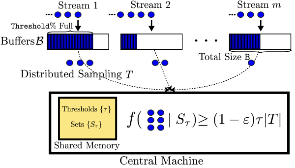
Figure 1: The schematic representation of our proposed hybrid algorithm: there are $m$ simultaneous streams where data from each stream is buffered separately. When a buffer is Threshold% full, a central machine starts the sampling process. The thresholds $\{\tau\}$ and sets $\{S_{\tau}\}$ are stored in a shared memory. First, for each threshold $\tau$, all elements with marginal gain less than $\tau$ are discarded from the buffers. Then the central machine randomly samples $t$ items $T$ (with geometrically increasing values of $t$) from the buffers of all streams and adds them to set $S_{\tau}$ if their average marginal gain is at least $(1-\varepsilon)\tau$. The sampling procedure stops when the average value of randomly picked items is not good enough. These iterative steps are performed until $k$ items are picked or the buffer memories of all machines are emptied.

Theorem 3.

For a non-negative and monotone submodular function $f$ in a multi-source streaming setting subject to a cardinality constraint $k$, define $\Delta_{0}$ as the largest singleton value when for the first time a buffer gets full, and $=/\frac{{\textup{{OPT}}}}{\Delta_{0}}$. The total communication cost of Batch-Sieve-Streaming++ is $O(\frac{k\log missing/missing}{\varepsilon^{2}})$.

Proof.

For $m$ different data streams, assume $\cB_{i}$ is the set of elements buffered from the $i$-th stream. We define $\cB$ to be the union of all elements from all streams. The communication cost of Batch-Sieve-Streaming++ in the multi-source setting is the total number of elements sampled (in a distributed way) from all sets $\{\cB_{i}\}_{1\leq i\leq m}$ in Lines 5 and 13 of Algorithm 3.

As a result, we can conclude that the communication cost is at most twice the number of elements has been in a set $S_{\tau}$ at a time during the run of the algorithm. To see the reason for this argument, note that because the filtering step happens just before the for loop of Lines 4–10, the first picked sample in this for loop always passes the test and is added to $S_{\tau}$. Furthermore, all the items sampled at Line 13, irrespective of their marginal gain, are added to $S_{\tau}$. So, in the worst case scenario, the communication complexity is maximum when the for loop breaks always at the second instance of the sampling process of Line 5 (after one successful try). Therefore, we only need to upper bound the total number of elements which at some point has been in a set $S_{\tau}$ at one of the calls to Threshold-Sampling.

The first group of thresholds the Batch-Sieve-Streaming++ algorithm considers the interval $[\nicefrac{{\Delta_{0}}}{{(2k)}},\Delta_{0}]$, where in the beginning we have $\texttt{LB}=\Delta_{0}$. Following the same arguments as the proof of Theorem 1, we can show that if neither LB nor $\Delta$ changes, the total number of elements in sets $\{S_{\tau}\}$ is $O(\frac{k}{\varepsilon})$. We define $\Delta_{\max}$ to be the largest singleton element in the whole data streams. The number of times the interval of thresholds changes because of the change in $\Delta$ is $\log_{1+\varepsilon}(\nicefrac{{\Delta_{\max}}}{{\Delta_{0}}})$. Furthermore, by changes in LB some thresholds and their corresponding sets are deleted and new elements might be added. The number of times LB changes is upper bounded by $\log_{1+\varepsilon}(\nicefrac{{\texttt{OPT}}}{{\Delta_{0}}})$. Note that we have $\Delta_{\max}\leq\texttt{OPT}$. From the fact that the number of changes in the set of thresholds is upper bounded by $\log_{1+\varepsilon}(\nicefrac{{\Delta_{\max}}}{{\Delta_{0}}})=O(\frac{\log missing/missing}{\varepsilon})$ and the number of elements in $\{S_{\tau}\}$ at every step of the algorithm is $O(\frac{k}{e})$, we conclude the total communication cost of Batch-Sieve-Streaming++ is $O(\frac{k\log missing/missing}{\varepsilon^{2}})$. ∎

5 Experiments

In these experiments, we have three main goals:

1. For the single-source streaming scenario, we want to demonstrate the memory efficiency of Sieve-Streaming++ relative to Sieve-Streaming.

2. For the multi-source setting, we want to showcase how Batch-Sieve-Streaming++ requires the fewest adaptive rounds amongst algorithms with optimal communication costs.

3. Lastly, we want to illustrate how a simple variation of Batch-Sieve-Streaming++ can trade off communication cost for adaptivity, thus allowing the user to find the best balance for their particular problem.

5.1 Datasets

These experiments will be run on a Twitter stream summarization task and a YouTube Video summarization task, as described next.

Twitter Stream Summarization

In this application, we want to produce real-time summaries for Twitter feeds. As of January 2019, six of the top fifty Twitter accounts (also known as “handles”) are dedicated primarily to news reporting. Each of these handles has over thirty million followers, and there are many other news handles with tens of millions of followers as well. Naturally, such accounts commonly share the same stories. Whether we want to provide a periodic synopsis of major events or simply to reduce the clutter in a user’s feed, it would be very valuable if we could produce a succinct summary that still relays all the important information.

To collect the data, we scraped recent tweets from 30 different popular news accounts, giving us a total of 42,104 unique tweets. In the multi-source experiments, we assume that each machine is scraping one page of tweets, so we have 30 different streams to consider.

We want to define a submodular function that covers the important stories of the day without redundancy. To this end, we extract the keywords from each tweet and weight them proportionally to the number of retweets the post received. In order to encourage diversity in a selected set of tweets, we take the square root of the value assigned to each keyword. More formally, consider a function $f$ defined over a ground set $V$ of tweets. Each tweet $e\in V$ consists of a positive value $\text{val}_{e}$ denoting its number of retweets and a set of $\ell_{e}$ keywords $W_{e}=\{w_{e,1},\cdots,w_{e,\ell_{e}}\}$ from a general set of keywords $\cW$. The score of a word $w\in W_{e}$ for a tweet $e$ is defined by $\text{score}(w,e)=\text{val}_{e}$. If $w\notin W_{e}$, we define $\text{score}(w,e)=0$. For a set $S\subseteq V$ of tweets, the function $f$ is defined as follows:

$$f(S)=\sum_{w\in\cW}\sqrt{\sum_{e\in S}\text{score}(w,e)}.$$

Figure 2 demonstrates how we calculate the utility of a set of tweets. In Appendix B, we give proof of submodularity of this function.

 

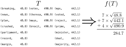
Figure 2: At the top, we show two tweets on the same subject from different accounts. We first extract the list of keywords, as well as the number of retweets per word. We combine these into a single list $T$ of (keyword, score) pairs and then pass this list through our submodular function $f$.

YouTube Video Summarization

In this second task, we want to select representative frames from multiple simultaneous and related video feeds. In particular, we consider YouTube videos of New Year’s Eve celebrations from ten different cities around the world. Although the cities are not all in the same time zone, in our multi-source experiments we assume that we have one machine processing each video simultaneously.

Using the first 30 seconds of each video, we train an autoencoder that compresses each frame into a 4-dimensional representative vector. Given a ground set $V$ of such vectors, we define a matrix $M$ such that $M_{ij}=e^{-\text{dist}(v_{i},v_{j})}$, where $\text{dist}(v_{i},v_{j})$ is the euclidean distance between vectors $v_{i},v_{j}\in V$. Intuitively, $M_{ij}$ encodes the similarity between the frames represented by $v_{i}$ and $v_{j}$.

The utility of a set $S\subseteq V$ is defined as a non-negative monotone submodular objective $f(S)=\log\det(I+\alpha M_{S})$, where $I$ is the identity matrix, $\alpha>0$ and $M_{S}$ is the principal sub-matrix of $M$ indexed by $S$ (Herbrich et al., 2003). Informally, this function is meant to measure the diversity of the vectors in $S$. Figure 3 shows the representative images selected by our Batch-Sieve-Streaming++ algorithm for $k=8$.

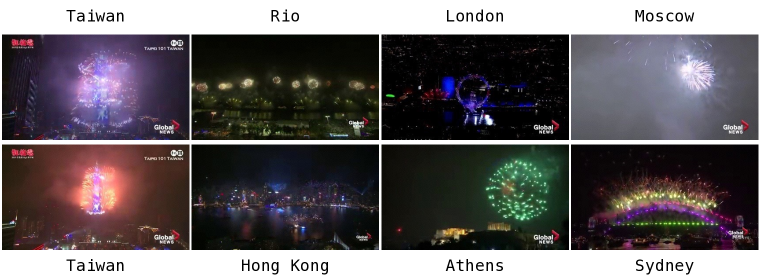
Figure 3: Eight representative frames chosen by Batch-Sieve-Streaming++ from ten different simultaneous feeds of New Year’s Eve fireworks from around the world.

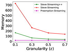
(a)

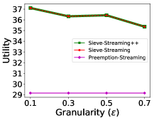
(b)

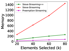
(c)

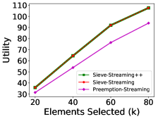
(d)

Figure 4: Graphs showing how the memory and utility of various single-source streaming algorithms vary with the cardinality $k$ and the granularity parameter $\varepsilon$. Note that the utility of Sieve-Streaming++ and Sieve-Streaming are exactly overlapping. In (a) and (b) we use k = 20, while in (c) and (d) we use $\varepsilon=0.3$.

5.2 Single-Source Experiments

In this section, we want to emphasize the power of Sieve-Streaming++ in the single-source streaming scenario. As discussed earlier, the two existing standard approaches for monotone $k$-cardinality submodular streaming are Sieve-Streaming and Preemption-Streaming.

As mentioned in Section 3, Sieve-Streaming++ theoretically has the best properties of both of these existing baselines, with optimal memory complexity and the optimal approximation guarantee. Figure 4 shows the performance of these three algorithms on the YouTube video summarization task and confirms that this holds in practice as well.

For the purposes of this test, we simply combined the different video feeds into one single stream. We see that the memory required by Sieve-Streaming++ is much smaller than the memory required by Sieve-Streaming, but it still achieves the exact same utility. Furthermore, the memory requirement of Sieve-Streaming++ is within a constant factor of Preemption-Streaming, while its utility is much better. The Twitter experiment gives similar results so those graphs are deferred to Appendix C.

5.3 Multi-Source Experiments

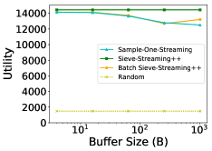
(a)

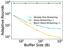
(b)

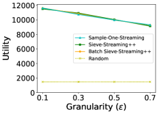
(c)

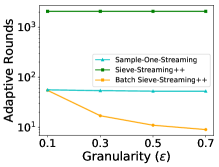
(d)

Figure 5: Graphs showing how the utility and adaptivity of various multi-source streaming algorithms vary with the buffer size B and the granularity $\varepsilon$. Unless they are being varied on the x-axis, we set $\varepsilon=0.7$, $\texttt{B}=100$, and $k=50$.

Once we move into the multi-source setting, the communication cost of algorithms becomes a key concern also. In this section, we compare the performance of algorithms in terms of utility and adaptivity where their communication cost is optimal.

Our first baseline is a trivial extension of Sieve-Streaming++. The multi-source extension for this algorithm essentially functions by locally computing the marginal gain of each incoming element, and only communicating it to the central machine if the marginal gain is above the desired threshold. However, as mentioned at the beginning Section 3.1, this algorithm requires $\Omega(n)$ adaptive rounds. Our second baseline is Sample-One-Streaming, which was described in Section 3.2.

Figures 5a and 5b show the effect of the buffer size B on the performance of these algorithms for the Twitter task. The main observation is that Batch-Sieve-Streaming++ can achieve roughly the same utility as the two baselines with many fewer adaptive rounds. Note that the number of adaptive rounds is shown in log scale.

Figures 5c and 5d show how these numbers vary with $\varepsilon$. Again, the utilities of the three baselines are similar. We also see that increasing $\varepsilon$ results in a large drop in the number of adaptive rounds for Batch-Sieve-Streaming++, but not for Sample-One-Streaming. Appendix C gives some additional graphs, as well as the results for the YouTube dataset.

5.4 Trade-off Between Communication and Adaptivity

In the multi-source setting, there is a natural exchange between communication cost and adaptivity. Intuitively, the idea is that if we sample items more aggressively (which translates into higher communication cost), a set $S$ of $k$ items is generally picked faster, thus it reduces the adaptivity. In the real world, the preference for one or the other can depend on a wide variety of factors ranging from resource constraints to the requirements of the particular problem.

In Threshold-Sampling, we ensure the optimal communication performance by sampling $t_{i}=\lceil(1+\varepsilon)^{i+1}-(1+\varepsilon)^{i}\rceil$ items in each step of the for loop. Instead, to reduce the adaptivity by a factor of $\log(k)$, we could sample all the required $k$ items in a single step. Thus, in one adaptive round we mimic the two for loops of Threshold-Sampling. Doing this in each call to Algorithm 3 would reduce the expected adaptive complexity of Threshold-Sampling to the optimal $\log(\texttt{B})$, but dramatically increase the communication cost to $O(k\log\texttt{B})$.

In order to trade off between communication and adaptivity, we can instead sample $t^{R}_{i}=\lceil(1+\varepsilon)^{i+R}-(1+\varepsilon)^{i}\rceil$ elements to perform $R$ consecutive adaptive rounds in only one round. However, to maintain the same chance of a successful sampling, we still need to check the marginal gain. Finally, we pick a batch of the largest size $t^{j}_{i}$ such that the average marginal gain of the first $t^{j-1}_{i}$ items is above the desired threshold. Then we just add just this subset to $S_{\tau}$, meaning we have wasted $\lceil(1+\varepsilon)^{i+R}-(1+\varepsilon)^{i+j}\rceil$ communication.

Scatter plots of Figure 6 shows how the number of adaptive rounds varies with the communication cost. Each individual dot represents a single run of the algorithm on a different subset of the data. The different colors cluster the dots into groups based on the value of $R$ that we used in that run. Note that the parameter $R$ controls the communication cost.

The plot on the left comes from the Twitter experiment, while the plot on the right comes from the YouTube experiment. Although the shapes of the clusters are different in the two experiments, we see that increasing $R$ increases the communication cost, but also decreases the number of adaptive rounds, as expected.

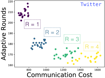
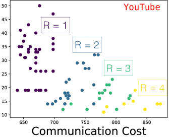
Figure 6: Scatter plots showing how we can lower the number of adaptive rounds by increasing communication. Each dot is the result of a single run of the algorithm and the colored clusters represent a particular setting for $R$.

6 Implications of Sieve-Streaming++ on Other Problems

Recently, there has been several successful instances of using the sieving idea proposed by Badanidiyuru et al. (2014) for designing streaming algorithms for a wide range of submodular maximization problems. In Section 3, we showed Sieve-Streaming++ (see Algorithm 1 and Theorem 1) reduces the memory complexity of streaming submodular maximization to $O(k)$. In this final section, we discuss how the approach of Sieve-Streaming++ significantly improves the memory complexity for several previously studied important problems.

Random Order Streams

Norouzi-Fard et al. (2018) studied streaming submodular maximization under the assumption that elements of a stream arrive in random order. They introduced a streaming algorithm called SALSA with an approximation guarantee better than $\nicefrac{{1}}{{2}}$. This algorithm uses $O(k\log(k))$ memory. In a very straightforward way, similarly to the idea of Sieve-Streaming for lower bounding the optimum value, we are able to improve the memory complexity of this algorithm to $O(k)$. Furthermore, Norouzi-Fard et al. (2018) introduced a $p$-pass algorithm ($p\geq 2$) for submodular maximization subject to a cardinality constraint $k$. We can also reduce the memory of this $p$-pass algorithm by a factor $\log(k)$.

Deletion-Robust

Mirzasoleiman et al. (2017) have introduced a streaming algorithm for the deletion-robust submodular maximization. Their algorithm provides a summary $S$ of size $O(kd\log(k)/\varepsilon)$ where it is robust to deletion of any set $D$ of at most $d$ items. Kazemi et al. (2018) were able to reduce the size of the deletion-robust summary to $O(k\log(k)/\varepsilon+d\log^{2}(k)/\varepsilon^{3})$. The idea of Sieve-Streaming++ for estimating the value of OPT reduces the memory complexities of these two algorithms to $O(kd/\varepsilon)$ and $O(k/\varepsilon+d\log^{2}(k)/\varepsilon^{3})$, respectively. It is also possible to reduce the memory complexity of STAR-T-GREEDY (Mitrovic et al., 2017b) by at least a factor of $\log(k)$.

Two-Stage

Mitrovic et al. (2018) introduced a streaming algorithm called Replacement-Streaming for the two-stage submodular maximization problem which is originally proposed by (Balkanski et al., 2016; Stan et al., 2017). The memory complexity of Replacement-Streaming is $O(\frac{\ell\log\ell}{\varepsilon})$, where $\ell$ is the size of the produced summary. Again, by applying the idea of Sieve-Streaming++ for guessing the value of OPT and analysis similar to the proof of Theorem 1, we can reduce the memory complexity of the streaming two-stage submodular maximization to $O(\frac{\ell}{\varepsilon})$.

Streaming Weak Submodularity

Weak submodular functions generalize the diminishing returns property.

Definition 1 (Weakly Submodular (Das and Kempe, 2011)).

A monotone and non-negative set function $f:2^{V}\rightarrow\bR_{\geq 0}$ is $\gamma$–weakly submodular if for each sets $A,B\subset V$, we have

$$\gamma\leq\frac{\sum_{e\in A\setminus B}f(\{e\}\mid B)}{f(A\mid B)},$$

where the ratio is considered to be equal to $1$ when its numerator and denominator are $0$.

It is straightforward to show that $f$ is submodular if and only if $\gamma=1$. In the streaming context subject to a cardinality constraint $k$, Elenberg et al. (2017) designed an algorithm with a constant factor approximation for $\gamma$–weakly submodular functions. The memory complexity of their algorithm is $O(\frac{k\log k}{\varepsilon})$. By adopting the idea of Sieve-Streaming++, we could reduce the memory complexity of their algorithm to $O(\frac{k}{\varepsilon})$.

Table 2 provides a summary of algorithms that we could significantly improve their memory complexity, while their approximation factors are maintained.

Table 2: Improved results for several other recently studied submodular maximization problems. The main idea of Sieve-Streaming++ enables us to significantly reduce the memory complexity of these problems.

Problem	Algorithm	Old Memory	New Memory	Ref.
Streaming	Salsa	$O(k\log(k))$	$O(k)$	Norouzi-Fard et al. (2018)
Streaming	P-PASS	$O(\nicefrac{{k\log(k)}}{{\varepsilon}})$	$O(\nicefrac{{k}}{{\varepsilon}})$	Norouzi-Fard et al. (2018)
Weak submodular	Streak	$O(\nicefrac{{k\log(k)}}{{\varepsilon}})$	$O(\nicefrac{{k}}{{\varepsilon}})$	Elenberg et al. (2017)
Deletion-Robust	ROBUST	$O(\nicefrac{{kd\log(k)}}{{\varepsilon}})$	$O(\nicefrac{{kd}}{{\varepsilon}})$	Mirzasoleiman et al. (2017)
Deletion-Robust	ROBUST-STREAM	$O(\nicefrac{{k\log(k)}}{{\varepsilon}}+\nicefrac{{d\log^{2}(k)}}{{\varepsilon^{3})}}$	$O(\nicefrac{{k}}{{\varepsilon}}+\nicefrac{{d\log^{2}(k)}}{{\varepsilon^{3})}}$	Kazemi et al. (2018)
Two-Stage	REPLACE-STREAM	$O(\nicefrac{{\ell\log(\ell)}}{{\varepsilon}})$	$O(\nicefrac{{\ell}}{{\varepsilon}})$	Mitrovic et al. (2018)

7 Conclusion

In this paper, we studied the problem of maximizing a non-negative submodular function over a multi-source stream of data subject to a cardinality constraint $k$. We first proposed Sieve-Streaming++ with the optimum approximation factor and memory complexity for a single stream of data. Build upon this idea, we designed an algorithm for multi-source streaming setting with a $\nicefrac{{1}}{{2}}$ approximation factor, $O(k)$ memory complexity, a very low communication cost, and near-optimal adaptivity. We evaluated the performance of our algorithms on two real-world data sets of multi-source tweet streams and video streams. Furthermore, by using the main idea of Sieve-Streaming++, we significantly improved the memory complexity of several important submodular maximization problems.

Acknowledgements.

The work of Amin Karbasi is supported by AFOSR Young Investigator Award (FA9550-18-1-0160) and Grainger Award (PO 2000008083 2016012). We would like to thank Ola Svensson for his comment on the first version of this manuscript.

Appendix A Proof of Lemma 1

Proof.

Since we are only adding elements to $S$, using submodularity the marginal value of any element $x$ to $S$, i.e. $f(x\mid S)$, is decreasing. Therefore, once an element is removed from the buffer $\cB$, it never comes back. As a result, the set $\cB$ is shrinking over time. When $\cB$ becomes empty, the algorithm terminates. Therefore it suffices to show that in every iteration of the while loop, a constant fraction of elements will be removed from $\cB$ in expectation. The rest of the analysis follows by analyzing the expected size of $\cB$ over time and applying Markov’s inequality.

We note that to avoid confusion, we call one round of the while loop in Lines 3–19 of Threshold-Sampling an iteration. There are two other internal for loops at Lines 4–10 and Lines 11–19. Later in the proof, we call each run of these for loops a step. There are $\lceil\frac{1}{\varepsilon}\rceil$ steps in the first for loop and $O(\log(k))$ steps in the second.

If an iteration ends with growing $S$ into a size $k$ set, that is going to be the final iteration as the algorithm Threshold-Sampling because the algorithm terminates once $k$ elements are selected. So we focus on the other case. An iteration breaks (finishes) either in the first for the loop at Lines 4–10 or in the second for loop of Lines 11–19. We say an iteration fails if after termination less than $\varepsilon/2$ fraction of elements in $\cB$ is removed. For iteration ${\ell}$, let $\cB^{\ell}$ be the set $\cB$ at Line 3 at the beginning of this iteration. So the first set $\cB^{1}$ consists of all the input elements passed to Threshold-Sampling. So we can say that an iteration ${\ell}$ fails if $|\cB^{{\ell}+1}|$ is greater than $(1-\varepsilon/2)\cdot|\cB^{\ell}|$.

Failure of an iteration can happen in any of the $\lceil\frac{1}{\varepsilon}\rceil+O(\log(k))$ steps of the two for loops. For each step $1\leq z\leq\lceil\frac{1}{\varepsilon}\rceil+O(\log(k))$, we denote the probability that the current iteration is terminated at step $z$ at a failed state with $P_{z}$. The probability that an iteration will not fail can then be written as

$$\prod_{z}(1-P_{z}).$$

In the rest of the proof, we show that this quantity is at least a constant for any constant $\varepsilon>0$.

First, we show that at any of the $\lceil\frac{1}{\varepsilon}\rceil$ steps of the first for loop, the probability of failing is less than $\varepsilon/2$. Let us consider step $1\leq z\leq\lceil\frac{1}{\varepsilon}\rceil$. We focus on the beginning of step $z$ and upper bound $P_{z}$ for any possible outcome of the previous steps $1,\cdots,z-1$. Let $S$ be the set of selected elements in all the first $z-1$ steps. If at least $\varepsilon/2$ fraction of elements in $\cB^{\ell}$ has a marginal value less than $\tau$ to $S$, we can say that the iteration will not fail for the rest of the steps for sure (with probability $1$). We note that as $S$ grows the marginal values of elements to it will not increase, so at least $\varepsilon/2$ fraction of elements will be filtered out independent of which step the process terminates.

So we focus on the case that less than $\varepsilon/2$ fraction of elements in $\cB^{\ell}$ have marginal value less than $\tau$ to $S$. Since, in the first loop, we pick one of them randomly and look at its marginal value as a test to whether terminate the iteration or not, the probability of termination at this step $z$ is not more than $\varepsilon/2$ and therefore $P_{z}$ is also at most $\varepsilon/2$.

In the second for loop, at Lines 11–19, we have a logarithmic number of steps and we can upper bound the probability of terminating the iteration in a failed state at any of these steps in a similar way. The main difference is that instead of sampling one random element from $\cB$, we pick $t$ random elements and look at their average marginal value together as a test to whether terminate the current iteration or not.

We want to upper bound the probability of terminating the iteration in a step $z>\lceil\frac{1}{\varepsilon}\rceil$ at a failed state. This will happen if at the step $z$ the Threshold-Sampling algorithm picks a random subset $T$ with

• $\dfrac{f(T\mid S)}{|T|}\leq(1-\varepsilon)\tau$, and

• also less than $\varepsilon/2$ fraction of elements in $\cB^{\ell}$ has a marginal value less than $\tau$ to $T\cup S$.

We look at the process of sampling $T$ as a sequential process in which we pick $t$ random elements one by one. We can call each of these $t$ parts a small random experiment. We note that the first property above holds only if in at least $\varepsilon t$ of these smaller random experiments the marginal value of the selected element to the current set $S$ is below $\tau$. We also assume that we add the selected elements to $S$ as we move on. We simulate this random process with a binomial process of tossing $t$ independent coins. If the marginal value of the $i$-th sampled element to $S$ is at least $\tau$, we say that the associated coin toss is a head. Otherwise, we call it a tail. The probability of a tail depends on the fraction of elements in $\cB^{\ell}$ with marginal value less than $\tau$ to $S$. If this fraction at any point is at least $\varepsilon/2$, we know that the second necessary property for a failed iteration does not hold anymore and will not hold for the rest of the steps. Therefore the failure happens only if we face at least $\varepsilon t$ tails each with probability at most $\varepsilon/2$. The rest of the analysis is applying simple concentration bounds for different values of $t$.

So we have a binomial distribution with $t$ trials each with head probability at least $1-\varepsilon/2$, and we want to upper bound the probability that we get at least $\varepsilon t$ tails. The expected number of tails is not more than $\varepsilon t/2$ so using Markov’s inequality, the probability of seeing at least $\varepsilon t$ tails is at most $0.5$. Furthermore, for larger values of $t$ we can have much better concentration bounds.

Using Chernoff type bounds in Lemma 2, we know the probability of observing at least $\varepsilon t$ tails is not more than:

$$P_{z}\leq\Pr\left(\textrm{tails}-\varepsilon t/2\geq\varepsilon t/2\right)\leq e^{-\varepsilon t/10}.$$

As we proceed in steps, the number of samples $t$ grows geometrically. Consequently, the failure probability declines exponentially (double exponential in the limit).

So the number of steps it takes to reach the failure probability declining phase is a function of $\varepsilon$ and therefore it is a constant number. We conclude that for any constant $\varepsilon>0$, the probability of not failing in an iteration, i.e., $\prod_{z}(1-P_{z})$, is lower bounded by a constant $\zeta_{\varepsilon}>0$. Since any iteration will terminate eventually, we can say that for any iteration with constant probability an $\varepsilon/2$ fraction of elements will be filtered out of $\cB$. So the expected size of $\cB$ after $X$ iterations will be at most $2^{-\Omega(X)}n$ where $n$ is the number of input elements at the beginning of Threshold-Sampling. So the probability of having more than $C\log(|\cB|)$ iterations decreases exponentially with $C$ for any coefficient $C$ using Markov’s inequality which means the expected number of iterations is $O(\log(|\cB|))$. ∎

Lemma 2 (Chernoff bounds, Bansal and Sviridenko [2006]).

Suppose $X_{1},\dots,X_{n}$ are binary random variables such that $\Pr\left(X_{i}=1\right)=p_{i}$. Let $\mu=\sum_{i=1}^{n}p_{i}$ and $X=\sum_{i=1}^{n}X_{i}$. Then for any $a>0$, we have

$$\Pr\left(X-\mu\geq a\right)\leq e^{-a\min\left(\frac{1}{5},\frac{a}{4\mu}\right)}.$$

Moreover, for any $a>0$, we have

$$\Pr\left(X-\mu\leq-a\right)\leq e^{-\frac{a^{2}}{2\mu}}.$$

Appendix B Twitter Dataset Details

B.1 Intuition

To clean the data, we removed punctuation and common English words (known as stop words, thus leaving each individual tweet as a list of keywords with a particular timestamp. To give additional value to more popular posts, we also saved the number of retweets each post received.

Therefore, any individual tweet $t$ consists of a set of keywords $K_{t}$ and a value $v_{t}$ that is the number of retweets divided by the number of words in the post.

A set of tweets $T$ can be thought of as a list of $(keyword,score)$ pairs. The keywords $K_{T}$ in a set $T$ is simply a union of the keywords of the tweets in T:

$$K_{T}=\bigcup_{t\in T}K_{t}$$

The score $s_{k}$ of each keyword $k\in K_{T}$ is simply the sum of the values of posts containing that keyword. That is, if $T_{k}\subseteq T$ is the subset of tweets in $T$ containing the keyword $k$, then:

$$s_{k}=\sum_{t\in T_{k}}v_{t}$$

Therefore, we define our submodular function $f$ as follows:

$$f(T)=\sum_{k\in K_{T}}\sqrt{s_{k}}$$

Intuitively, we sum over all the keyword scores because we want our set of tweets to cover as many high-value keywords as possible. However, we also use the square root to introduce a notion of diminishing returns because once a keyword already has a high score, we would prefer to diversify instead of further picking similar tweets.

B.2 General Formalization

In this section, we first rigorously define the function used for Twitter stream summarization in Section 5.1. We then prove this function is non-negative and monotone submodular.

Function Definition

Consider a function $f$ defined over a ground set $V$ of items. Each item $e\in V$ consists of a positive value $\text{val}_{e}$ and a set of $\ell_{e}$ keywords $W_{e}=\{w_{e,1},\cdots,w_{e,\ell_{e}}\}$ from a general set of keywords $\cW$. The score of a word $w\in W_{e}$ for an item $e$ is defined by $\text{score}(w,e)=\text{val}_{e}$. If $w\notin W_{e}$, we define $\text{score}(w,e)=0$. For a set $S\subseteq V$ the function $f$ is defined as follows:

$$f(S)=\sum_{w\in\cW}\sqrt{\sum_{e\in S}\text{score}(w,e)}.$$ (2)

Lemma 3.

The function $f$ defined in Eq. (2) is non-negative and monotone submodular.

Proof.

The not-negativity and monotonicity of $f$ are trivial. For two sets $A\subset B$ and $e\in V\setminus B$ we show that

$$f(\{e\}\cup A)-f(A)\geq f(\{e\}\cup B)-f(B).$$

To prove the above inequality, assume $W_{e}=\{w_{e,1},\cdots,w_{e,\ell_{e}}\}$ is the set of keywords of $e$. For a keyword $w_{e,i}$ define $a_{w_{e,i}}=\sum_{u\in A}\text{score}(w_{e,i},u)$ and $b_{w_{e,i}}=\sum_{u\in B}\text{score}(w_{e,i},u)$. It is obvious that $a_{w_{e,i}}\leq b_{w_{e,i}}$. It is straightforward to show that

$$\textstyle\sqrt{a_{w_{e,i}}+\text{score}(w_{e,i},e)}-\sqrt{a_{w_{e,i}}}\geq\sqrt{b_{w_{e,i}}+\text{score}(w_{e,i},u)}-\sqrt{b_{w_{e,i}}}.$$

If sum over all keywords in $W_{e}$ then the submodularity of $f$ is proven. ∎

Appendix C More Experimental Results

In this section, we will present a few more graphs that we didn’t have space for in the main paper.

C.1 Single-Source Experiments

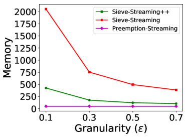
(a)

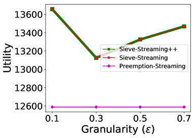
(b)

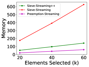
(c)

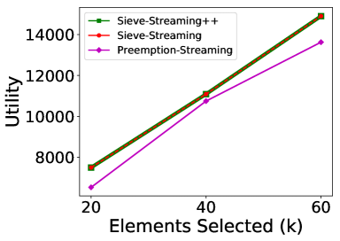
(d)

Figure 7: Single-source streaming results on the Twitter summarizaton task. In (a) and (b), $\varepsilon=0.5$. In (c) and (d), $k=50$.

Here we present the set of graphs that we displayed in Figure 4, except here they are run on the Twitter dataset instead. For the most part, they are showing the same trends we saw before. Sieve-Streaming++ has the exact same utility as Sieve-Streaming, which is better than Preemption-Streaming. We also see the memory requirement of Sieve-Streaming++ is much lower than that of Sieve-Streaming, as we had hoped.

The only real difference is in the shape of the utility curve as $\varepsilon$ varies. In Figure 4, the utility was decreasing as $\varepsilon$ increased, which is not necessarily the case here. However, this is relatively standard because changing $\varepsilon$ completely changes the set of thresholds kept by Sieve-Streaming++, so although it usually helps the utility, it is not necessarily guaranteed to do so.

Also, note that we only went up to $k=60$ in this experiment because Preemption-Streaming was prohibitively slow for larger $k$.

C.2 Multi-Source Experiments

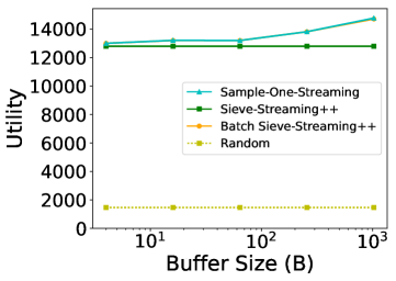
(a)

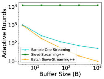
(b)

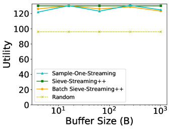
(c)

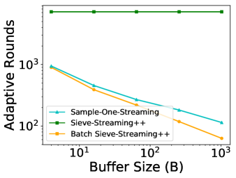
(d)

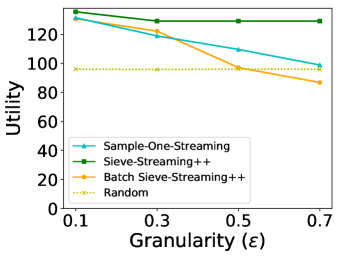
(e)

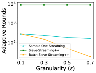
(f)

Figure 8: Additional multi-source graphs. (a) and (b) are additional graphs for the Twitter dataset, this time with $\varepsilon=0.6$ and $k=50$. (c) through (f) are the equivalent of Figure 5, but for the YouTube dataset. Unless they are being varied on the x-axis, we set $\varepsilon=0.25$, $\texttt{B}=100$, and $k=100$.

In Figure 5a, Sieve-Streaming++ had the best utility performance. In Figure 8a, we set $k=50$ and $\varepsilon=0.6$ and now we see that Batch-Sieve-Streaming++ and Sample-One-Streaming have higher utility, and that this utility increases as the buffer size increases. However, in this case too, the main message is that the utilities of the three algorithms are comparable, but Batch-Sieve-Streaming++ uses the fewest adaptive rounds (Figure 5b).

In Figures 8c through 8f, we display the same set of graphs as Figure 5, but for the YouTube experiment. In the YouTube experiment, it is more difficult to select a set of items that is significantly better than random, so we need to use a smaller value of $\varepsilon$. We see that for smaller $\varepsilon$, the difference in adaptive rounds between Batch-Sieve-Streaming++ and Sample-One-Streaming is smaller. This is consistent with our results because the number of adaptive rounds required by Sample-One-Streaming does not change much with $\varepsilon$, while the number of adaptive rounds of Batch-Sieve-Streaming++ increases as $\varepsilon$ gets smaller.

References

- Badanidiyuru and Vondrák [2014] Ashwinkumar Badanidiyuru and Jan Vondrák. Fast algorithms for maximizing submodular functions. In Symposium on Discrete Algorithms, SODA, pages 1497–1514, 2014.