Recombinator-$k$-means: An evolutionary algorithm that exploits $k$-means++ for recombination

Abstract

We introduce an evolutionary algorithm called recombinator-$k$-means for optimizing the highly non-convex kmeans problem. Its defining feature is that its crossover step involves all the members of the current generation, stochastically recombining them with a repurposed variant of the $k$-means++ seeding algorithm. The recombination also uses a reweighting mechanism that realizes a progressively sharper stochastic selection policy and ensures that the population eventually coalesces into a single solution. We compare this scheme with state-of-the-art alternative, a more standard genetic algorithm with deterministic pairwise-nearest-neighbor crossover and an elitist selection policy, of which we also provide an augmented and efficient implementation. Extensive tests on large and challenging datasets (both synthetic and real-word) show that for fixed population sizes recombinator-$k$-means is generally superior in terms of the optimization objective, at the cost of a more expensive crossover step. When adjusting the population sizes of the two algorithms to match their running times, we find that for short times the (augmented) pairwise-nearest-neighbor method is always superior, while at longer times recombinator-$k$-means will match it and, on the most difficult examples, take over. We conclude that the reweighted whole-population recombination is more costly, but generally better at escaping local minima. Moreover, it is algorithmically simpler and more general (it could be applied even to $k$-medians or $k$-medoids, for example). Our implementations are publicly available at https://github.com/carlobaldassi/RecombinatorKMeans.jl.

I Introduction

The problem of minimizing the sum-of-squares error ($\mathrm{SSE}$) is a central and paradigmatic clustering problem in data science. It is usually addressed by some variant of the classical $k$-means heuristic [1, 2]. The SSE objective is most commonly defined as follows: given $N$ data points $\mathcal{X}=\left(x_{i}\right)_{i=1}^{N}$, where each point is $D$-dimensional, $x_{i}\in\mathbb{R}^{D}$, and given an integer $k\geq 2$, we wish to find $k$ centroids $\mathcal{C}=\left(c_{a}\right)_{a=1}^{k}\in\left(\mathbb{R}^{D}\right)^{k}$, and a partition of the data points $\mathcal{P}=\left(p_{i}\right)_{i=1}^{N}\in\left\{1,\dots,k\right\}^{N}$ that minimize the cost function:

$$\mathrm{SSE}\left(\mathcal{C},\mathcal{P};\mathcal{X}\right)=\sum_{i=1}^{N}\left\|x_{i}-c_{p_{i}}\right\|^{2}$$ (1)

It is straightforward to prove that, for fixed $\mathcal{C}$, the optimal partition is given by associating each point to its nearest centroid; conversely, for fixed $\mathcal{P}$, the optimal centroids are given by the barycenter of each cluster. Indeed, the standard algorithm used for optimization is Lloyd’s algorithm [3], commonly referred to simply as $k$-means, which, starting from an initial guess for the centroids (the so-called “seeding”) uses an alternating iterative strategy, optimizing the partition and the centroids in turn. This can be regarded as a local search strategy and it is guaranteed to reach a fixed point in a finite number of steps. However, the $\mathrm{SSE}$ function, when considered as a function of $\mathcal{C}$ alone (with $\mathcal{P}$ optimized away as explained above) is in general highly non-convex, and in fact the optimization problem is NP-hard [4]. As a result, $k$-means gets very easily stuck in local minima unless it is initialized close to the global optimum.

Proposals about how to deal with this issue abound in the literature [5, 6]. The most direct approach consists in trying to optimize the seeding. A basic (and computationally very cheap) seeding strategy, which is often implied when referring to “the $k$-means algorithm” without qualifiers, is to sample the initial centroids uniformly at random from $\mathcal{X}$ [7]. This often leads to poor results and long convergence times. Alternative, more refined schemes, e.g. $k$-means++ [8], generally trade off some computational time during the seeding procedure for faster convergence times and improved results. However, it is often the case under realistic circumstances that the optimization landscape is so highly non-convex and riddled with local minima that local search algorithms still yield very sub-optimal results, even with improved seeding.

When looking to go beyond local search strategies, evolutionary algorithms provide an appealing and successful general paradigm [9, 10, 11]. Indeed, several approaches tailored to clustering problems, in which the $\mathrm{SSE}$ cost is identified with the fitness, have been put forward [12]. In this paper, we investigate in detail two evolutionary algorithms: a novel one, called recombinator-$k$-means, that we detail below, and a genetic algorithm proposed in ref. [13] that we refer to as GA-$k$-means in this paper. They both follow this scheme: we maintain a population of $J$ individuals, from which a new generation is obtained by a crossover mechanism followed by local optimization of each individual (via Lloyd’s algorithm or any equivalent scheme), until some convergence criterion for the whole population is met. Because of the use of local optimization, this scheme could be categorized as memetic, rather than genetic [12, 14, 15].

The most peculiar feature of recombinator-$k$-means is its multiple-parent (in fact, population-wide) crossover mechanism, based on a repurposed variant of the $k$-means++ seeding algorithm. The basic idea is to pool together all the centroids of the current population, and to use $k$-means++ to “recombine” them, letting it choose centroids from different individuals. This produces new stochastic seeds that are pieced together from locally-optimal configurations of the previous generation, and which are then optimized locally again. On top of this basic mechanism, we adopt a $\left(\mu+\lambda\right)$-ES selection strategy for survival, ensuring that the average $\mathrm{SSE}$ of the population decreases monotonically at each generation. Furthermore, we employ a novel selection-for-variation strategy that gradually and self-adaptively drives the recombination from an exploration phase to an exploitation one. The combination of the two selection strategies guarantees that the population eventually coalesces into a single configuration, thereby providing a natural stopping criterion.

The main contributions of this work can be summarized as follows. 1) We present a new evolutionary algorithm for $\mathrm{SSE}$ optimization with an original crossover step and an original selection-for-variation policy; the former is easily generalizable to clustering problems in the same family, while the latter could in principle be exported easily to an even larger set of optimization problems. 2) We provide an efficient implementation of GA-$k$-means, and demonstrate the benefit of augmenting it with improved seeding for the generation of its initial population. 3) We present results on large realistic datasets in terms of the trade-off between optimization quality and time, in the hope of offering practically relevant insights.

The rest of the paper is organized as follows. In sec. II we set up the framework of our study in the context of prior literature. In sec. III we review the GA-$k$-means algorithm. In sec. IV we review the $k$-means++ seeding procedure, in particular an enhanced variant of it called greedy-kmeans++ that is seldom discussed in the literature. In sec. V we introduce our recombinator-$k$-means scheme. In sec. VI we present and analyze detailed numerical results on several challenging synthetic and non-synthetic datasets. Sec. VII has a final discussion.

II Framework and prior literature

In the general context of clustering, optimizing the $\mathrm{SSE}$ objective can be taxonomized as partitional (i.e. the clusters are non-overlapping) and non-hierarchical. It’s a hard combinatorial optimization problem with a wide range of applications, from data analysis to data compression. Indeed, the literature on optimizing the $\mathrm{SSE}$ objective is vast and covers a large variety of circumstances. In the present work, we do not consider any modified versions of the objective function (e.g. outlier detection mechanisms as in refs. [16, 17]). In particular, we will always assume the desired number of clusters $k$ to be part of the input to the problem.

We further focus our attention on situations in which local optimization (one run of seeding+Lloyd’s algorithm) is significantly sub-optimal (i.e. it has a zero or very low chance of approximating well the global optimum), and computational resources allow to perform local optimizations repeatedly. We want to consider fairly large datasets that pose a significant and challenging optimization problem; we will however assume that the data fits into memory, otherwise even Lloyd’s algorithm would not be practical. For huge datasets that don’t fit in memory, a techniques such as BIRCH [16], that lossily compresses the data by pre-clustering it as it reads it, could still be employed; any standard $\mathrm{SSE}$ optimization technique could then be applied to the compressed representation by just adding some weights in eq. (1). We also always assume the data to be in a dense format, since sparse data generally requires specialized techniques, e.g. [18].

Under these circumstances, using an evolutionary strategy looks promising, and indeed, as mentioned in the introduction, many proposals of this kind have been put forward. A survey of such approaches can be found for example in ref. [12]. Most of the approaches can be more specifically categorized as genetic algorithms, and basically all of them use so-called cluster-oriented operators, meaning that they are specialized to the task at hand rather than using a task-independent meta-heuristic. They also all use a fixed population size across generations. Their distinguishing characteristics can be broken down into which specific choices were made for the key features and operators of simulated genetic evolution: 1) representation of the information about an individual (also called “chromosomes”) 2) construction of the initial population (generation $0$); 3) crossover (also called “recombination”) mechanism; 4) selection-for-variation policy (i.e. the relative weight of the parents in producing the offspring) and selection-for-survival policy (i.e. which individuals contribute to the next generation); 5) mutation step.

Some common traits emerge in many of these key features when surveying $\mathrm{SSE}$-optimizing algorithms. In particular, as far as we can tell: 1) The representation (chromosomes) uses either the centroids $\mathcal{C}$ or the partition $\mathcal{P}$, or both. This is natural since, as we have mentioned, either of the two can implicitly define the other. 2) The starting population is always some variant of random uniform sampling in some space. 3) The crossover step, when present, always uses at most two parent individuals, producing either one or two children. 4) The selection policies are most commonly, although not always, uniform for variation and either elitist or proportional to the fitness for selection. 5) The mutation step is more variable (e.g. perturbation of the centroids with random noise, random swapping of a centroid with a data point, reassigning a data point from one cluster to a nearby one), sometimes it is absent entirely.

The state-of-the-art in this area is, to the best of our knowledge, the genetic algorithm proposed by Fränti in ref. [13], that we refer to as GA-$k$-means. In summary, this method uses the full configuration $\left(\mathcal{C},\mathcal{P}\right)$ as representation, its initialization is based on a partition generated by picking centroids uniformly at random from the dataset, it employs an elitist policy for survival and uniform for variation, the (optional) mutation step is random swap of a centroid with a data point (after which the partition must be updated). Finally and most importantly, it uses deterministic pairwise-nearest-neighbor (PNN) crossover. We provide a detailed description of this method in the next section. Another algorithm, called self-adaptive genetic algorithm [19], purports to beat GA-$k$-means by using a meta-optimization strategy: it considers an array of genetic operators, assigns a combination of them to each individual, and applies the genetic evolution to those as well. While interesting, this strategy has an additional level of complexity and it is very expensive; the authors tests run for $1000$ generations and several hours on average, whereas we are interested in much shorter time scales (for the same type of data). Furthermore, the tests are performed at a fixed amount of generations, and the self-adaptive version takes between $1.5$ and $2$ times as much time. For these reasons, we don’t consider it in the present study.

When framed in the context of the existing literature, our recombinator-$k$-means algorithm (that we describe in detail in sec. V) shares the same general structure, but it is peculiar in several respects. Most prominently, the recombination/crossover mechanism (which uses the centroids $\mathcal{C}$ as its chromosomes) involves the whole population to generate each offspring, rather than just two parents. While using multiple parents isn’t unheard of in the context of genetic programming/evolutionary methods (see e.g. refs. [20, 21]), it is nevertheless uncommon. Our selection-for-variation policy is also novel and stands out from all other algorithms. Additionally, the arguments at the basis of our recombination method assume that the population consists of (nearly) local optima. For this reason, our initial population is not sampled uniformly at random but the result of local optimization, and we apply local optimization after each crossover step as well. Therefore, recombinator-$k$-means can be regarded as a memetic algorithm. The GA-$k$-means algorithm also uses local optimization (although in the original implementation it was capped at $2$ Lloyd’s iterations), and could be more precisely called memetic as well.

III Review of the genetic algorithm with deterministic PNN crossover

The main feature of GA-$k$-means is the use of the deterministic pairwise-nearest-neighbor (PNN) crossover, because it is particularly well-suited for implementation efficiency. For any two individuals, represented by their configurations $\left(\mathcal{C}_{1},\mathcal{P}_{1}\right)$ and $\left(\mathcal{C}_{2},\mathcal{P}_{2}\right)$, a new configuration is produced as follows. First, the configurations are merged into one with at most $2k$ centroids, obtained by $\mathcal{C}_{m}=\mathcal{C}_{1}\cup\mathcal{C}_{2}$; the optimal partition $\mathcal{P}_{m}$ is also easily computed. This step takes $O\left(kD+N\right)$ time. The second step is half of a Lloyd iteration: the centroids are updated based on $\mathcal{P}_{m}$. This takes $O\left(ND\right)$ time. The third step consists in iteratively merging pairs of clusters until only $k$ clusters remain. Merging two clusters means taking the union of the corresponding data points. As it turns out, thanks to the fact that the $\mathrm{SSE}$ uses the squared Euclidean distance, the centroid of the union is the average of the two centroids, weighted by the partition sizes. The two clusters to be merged at each turn are the “nearest-neighbors”, meaning those whose merging would increase the least the $\mathrm{SSE}$. The cost increase of merging two clusters can also be computed solely from their centroids and sizes, once again thanks to the properties of the $\mathrm{SSE}$. After each cluster merge, the merging costs of all other pairs need to be updated. By performing all the computations on the centroids alone, without the need to look at the data, we can save a factor $N$. Thus this third step requires $O\left(Dk^{2}\tau\right)$, where $\tau$ is related to the time required for the updates after each merge, and it is at most $O\left(k\right)$ but generally much lower in practice. After the merge operations have brought down the number of clusters to $k$, we still need a final step in which the partition information is updated based on the new centroids, which is the other half of a Lloyd iteration and takes $O\left(NDk\right)$.

Overall, the computational cost for producing an offspring from two configurations is $O\left(Dk^{2}\tau+NDk\right)$. This must be repeated $J$ times in order to produce the next generation.

The selection-for-survival mechanism of GA-$k$-means is elitist. For a given $J$, define $J_{e}=\left\lceil\left(1+\sqrt{1+8J}\right)/2\right\rceil$. In the elitist scheme, only the best $J_{e}$ members of the population produce offspring, by pairwise mating. If $J$ is a triangular number, then $J=J_{e}\left(J_{e}-1\right)/2$ and the new generation is obtained from all possible pairs in the “elite” subset. The fact that none of the two parents is favored in the crossover, and that all parents in the elite subset have the same number of children, means that the selection-for-variation policy is uniform. If $J$ is not a triangular number, only the first $J$ pairs (in lexicographic order) out of the elite subset are used, which introduces a slight bias towards fitter parents.

In ref. [13], each new configuration is optimized with at most $2$ additional Lloyd’s iterations. We found that $10$ gives a better time-cost trade-off. Also, the first generation is produced by choosing centroids uniformly at random from the data, and computing the corresponding partition. In our numerical experiments (see sec. VI) we will show that using a more expensive greedy-$k$-means++ seeding (see next section) followed by Lloyd’s algorithm (at most $10$ iterations) also consistently pays off in terms of the time-cost trade-off.

As mentioned above, genetic algorithms commonly employ a mutation mechanism to increase the genetic variation in the population. One such mechanism, based on randomly swapping a centroid for a data point, was explored in ref. [13], but the author recommends against it for performance reasons.

As a further optimization, the tests and code of ref. [13] use the technique introduced in ref. [22] to speed up Lloyd iterations, which is quite effective in saving some distance computations in the partition update after the first iteration, at the cost of keeping track of which centroids remain unchanged between one iteration and the next. We also use this technique throughout the paper.

IV Review of the (greedy)-$k$-means++ seeding procedure

Arguably [6], the most popular seeding method among those that go beyond uniform sampling is currently the so-called $k$-means++ method [8], due to its simplicity (conceptual and in terms of implementation), versatility, availability, relatively low computational cost $O\left(NDk\right)$, and generally good performances, especially if restarts are a viable option [5]. The procedure consists in sampling the centroids from the data points $\mathcal{X}$ progressively: the first one is sampled uniformly at random, while each new one is sampled with a probability proportional to the squared-distance from the nearest among the already-chosen centroids. This procedure can be refined by adding an extra sampling step: whenever a new centroid (besides the first one) needs to be selected, $s$ candidates are sampled, and the one that minimizes the cost function computed with the current number of centroids is kept. This is called greedy-$k$-means++ by Celebi et al. in ref. [5] (where they recommend it as one of the optimal choices for practical purposes when restarts are a viable option), but we were unable to find an original source for this algorithm. The details of the algorithm are provided as a special case of the reservoir-kmeans++ scheme discussed later, see Algorithm 1.

The parameter $s$ determines the amount of extra sampling. For $s=1$ we recover the basic $k$-means++ algorithm. In all our tests, we have used the default value used by the scikit-learn library, $s=\left\lfloor 2+\log k\right\rfloor$, which seems to provide a good trade-off between the improvement in the initial configuration and the extra computational time required. The computational complexity of this algorithm is $O\left(ksND\right)$.

V The recombinator-$k$-means scheme

As stated in the introduction, the basic idea of recombinator-$k$-means is to use greedy-$k$-means++ as a crossover step, applying it on the centroids pooled from a population of local optima. This idea stems from an empirical observation, which we summarize in the following. In Appendix -A we provide a detailed case-study analysis that demonstrates the mechanism in detail. Consider a case in which the data $\mathcal{X}$ is isotropically clustered around some centroids and the clusters are all about the same size and shape, and well separated from each other, and the number of clusters $k$ is known – in other words, a case for which the global minimizer of the $\mathrm{SSE}$ objective is very close to the ground truth. Due to the highly non-convex nature of the $\mathrm{SSE}$, a single run of a local optimization algorithm may still have a very low chance of “hitting” on the ground truth, even under such favorable circumstances, even if initialized with a good seeding technique such as greedy-$k$-means++ (we show this in sec. VI-B). In such context, the basic strategy of just repeating the optimization a number of times (known as “repeated-$k$-means” or “multi-start-$k$-means” [6]) can be very inefficient. On the other hand, the sub-optimality of each repeated try can often be ascribed to a few easily identifiable and mostly uncorrelated “mistakes”. Thus the centroids found in $J$ “unsuccessful” individual runs, when pooled together, are actually likely to be tightly clustered around the ground-truth centroids.

We can consider this pool of centroids as a new dataset that is mostly concentrated around $k$ very tight clusters (around the ground-truth centroids) with a few outliers (the “mistakes”, e.g. points lying between two ground-truth clusters). Running the greedy-$k$-means++ seeding on such dataset is very likely to only hit each and all of the tight clusters and ignore the outliers, for two reasons: 1) the centroids in the tight clusters have a higher chance of being selected, simply because they are in the majority; 2) once a centroid in one of the tight clusters is chosen, all the other centroids in the same cluster have a near-zero chance of being subsequently chosen, due to the $k$-means++ probability reweighting that goes like the square of the distance. The use of $s>1$ candidates in greedy-$k$-means++ further increases the chances of success. The overall effect is that of “recombining” the previous results and produce a nearly-optimal configuration with good probability.

Indeed, in such (quite artificial) situations it is often the case that a single recombination of very few results can solve the optimization problem, as we show in sec. VI-B. Perhaps surprisingly, this crossover step proves to be effective even in more realistic scenarios, producing configurations that, once locally optimized, are often significantly better than any of the input ones. If, when repeating the procedure several times, several new alternative configurations are produced, it is natural to consider iterating this process for several generations until no further progress can be made.

1:function reservoir-kmeans++($\mathcal{Y}$, $w$, $\mathcal{X}$, $k$, $s$)

2:     Initialize an empty list of centroids $\mathcal{C}$

3:     Sample the first centroid $c_{1}$ at random from $\mathcal{Y}$ with probability $P\left(y_{i}\right)\propto w_{i}$, and append it to $\mathcal{C}$

4:     for $a=2,\dots,k$ do

5:         $\phi^{\mathrm{best}}\leftarrow\infty$

6:         for $b=1,\dots,s$ do

7:              Sample candidate centroid $c^{\mathrm{cand}}$ from $\mathcal{Y}$ with probability $P\left(y_{i}\right)\propto w_{i}\min_{a^{\prime}<a}d\left(y_{i},c_{a^{\prime}}\right)^{2}$

8:              $\mathcal{C}^{\mathrm{cand}}\leftarrow$ append candidate $c^{\mathrm{cand}}$ to (a copy of) $\mathcal{C}$

9:              $\phi^{\mathrm{cand}}\leftarrow\mathrm{SSE}\left(\mathcal{C}^{\mathrm{cand}};\mathcal{X}\right)$

10:              if $\phi^{\mathrm{cand}}<\phi^{\mathrm{best}}$ then

11:                  $c^{\mathrm{best}}\leftarrow c^{\mathrm{cand}}$

12:                  $\phi^{\mathrm{best}}\leftarrow\phi^{\mathrm{cand}}$

13:              end if

14:         end for

15:         $\mathcal{C}\leftarrow$ append $c^{\mathrm{best}}$ to $\mathcal{C}$

16:     end for

17:     return $\mathcal{C}$

18:end function

1:function recombinator-kmeans($\mathcal{X}$, $k$, $J$, $s=\left\lfloor\log k+2\right\rfloor$, $\Delta\beta=0.1$, $t_{\mathrm{max}}=10$)

2:     $\mathcal{Y}\leftarrow\mathcal{X}$

3:     Initialize $w$ to a uniform vector, of the same length as $\mathcal{Y}$

4:     $\beta\leftarrow 0$

5:     $\phi^{\mathrm{best}}\leftarrow\infty$

6:     Initialize an empty list of configurations $\mathcal{K}$ and of costs $\Phi$

7:     repeat

8:         Initialize an empty list of configurations $\mathcal{K}^{\mathrm{new}}$ and of costs $\Phi^{\mathrm{new}}$

9:         for $r=1,\dots,J$ do

10:              $\mathcal{C}\leftarrow\textsc{reservoir-kmeans++}\left(\mathcal{Y},w,\mathcal{X},k,s\right)$

11:              $\mathcal{C}\leftarrow$ Run Lloyd’s algorithm on $\mathcal{X}$ with initial points $\mathcal{C}$ for at most $t_{\mathrm{max}}$ steps

12:              Compute $\phi=\mathrm{SSE}\left(\mathcal{C};\mathcal{X}\right)$ and append it to $\Phi^{\mathrm{new}}$

13:              Append $\mathcal{C}$ to $\mathcal{K}^{\mathrm{new}}$

14:              if $\phi<\phi^{\mathrm{best}}$ then

15:                  $\phi^{\mathrm{best}}\leftarrow\phi$

16:                  $\mathcal{C}^{\mathrm{best}}\leftarrow\mathcal{C}$

17:              end if

18:         end for

19:         $\Phi,\mathcal{K}\leftarrow\textsc{keepbest}\left(\Phi\cup\Phi^{\mathrm{new}},\mathcal{K}\cup\mathcal{K}^{\mathrm{new}},J\right)$

20:         $\beta\leftarrow\beta+\Delta\beta$

21:         $w\leftarrow\textsc{weights}\left(\Phi,\beta\right)$

22:         $\mathcal{Y}\leftarrow$ list of all the centroids in $\mathcal{K}$

23:     until $\mathrm{mean}\left(\Phi\right)\approx\min\left(\Phi\right)$

24:     return $\mathcal{C}^{\mathrm{best}}$

25:end function

Algorithm 1 Top: the reservoir-kmeans++ recombination algorithm. We have highlighted the differences with respect to greedy-kmeans++ in blue: the latter is recovered using $\mathcal{Y}=\mathcal{X}$ as the reservoir and uniform weights $w$; by also setting $s=1$ we recover the standard (non-greedy) kmeans++ algorithm.
Bottom: the recombinator-kmeans algorithm. The use of an approximate comparison in the stopping criterion (line 23) is intended to account for small (arguably irrelevant) differences. In our tests, we used a relative tolerance of $10^{-4}$. The functions keepbest and weights are discussed in the text. The default values for $s$, $\Delta\beta$ and $t_{\max}$, used throughout the paper, are shown in the argument list.

This basic idea can be improved by introducing a few adjustments to the greedy-$k$-means++ seeding algorithm to repurpose it for recombination; we call the resulting algorithm reservoir-$k$-means++, see the first function in Algorithm 1. It accepts a reservoir argument $\mathcal{Y}$: a list of points from which to sample the seeds, distinct from the data points $\mathcal{X}$. We still use the original data $\mathcal{X}$ in the cost function $\mathrm{SSE}$ to determine the best candidate among the $s$ samples at each step. There is one more extra argument, discussed below: a vector of weights $w$ of the same size as $\mathcal{Y}$, that can be used to favor some of the candidates in the reservoir over others, realizing a soft selection-for-variation policy. The computations can be carried out rather more efficiently than shown in the pseudocode, by employing appropriate data structures. For the greedy-kmeans++ special case (i.e., when $\mathcal{Y}=\mathcal{X}$), time scales as $O\left(kNDs\right)$, with $O\left(ND\right)$ additional memory. Using a reservoir with $kJ$ points instead we get $O\left(k\left(sN+kJ\right)D\right)$ time, with $O\left(kJD\right)$ extra memory. The two cases are comparable as long as $kJ$ is $O\left(N\right)$. The actual code is publicly available at ref. [25].

The second function in Algorithm. 1 is the recombinator-kmeans algorithm. It uses two additional auxiliary functions, keepbest and weights. The function keepbest$\left(\Phi^{\prime},\mathcal{K}^{\prime},J\right)$ returns the $J$ best costs in $\Phi^{\prime}$, along with their corresponding configurations found in $\mathcal{K}^{\prime}$. It is, in fact, a realization of the so-called $\left(\mu+\lambda\right)$ selection-for-survival procedure used in evolutionary strategies [26]. It guarantees that the population average monotonically improves at each generation.

The function weights determines the selection-for-variation bias that favors the centroids in $\mathcal{Y}$ belonging to configurations of smaller cost; it thus has the role of a fitness function. We introduce a novel heuristic for this purpose, that gradually increases the bias, starting from a low value to encourage initial exploration and variability, and progressively going towards an exploitation phase, ensuring that the batches eventually collapse onto some “consensus” configuration. In detail: given an array of costs $\Phi=\left(\phi_{a}\right)_{a=1}^{J}$, we compute the best $\phi^{\star}=\min_{a=1:J}\left(\phi_{a}\right)$ and the mean $\overline{\phi}=\frac{1}{J}\sum_{a=1}^{J}\phi_{a}$, and use the following formula to determine the weight of the centroids in a sample $a$:

$$w_{a}=\exp\left(-\beta\frac{\phi_{a}-\phi^{\star}}{\overline{\phi}-\phi^{\star}}\right)$$ (2)

with some parameter $\beta\geq 0$. This formula gives the largest weight to configurations close to the best one. Using the difference between the mean and the best as a scale in the denominator makes the function self-adaptive. The parameter $\beta$ determines the amount of skew in the weights, with $\beta=0$ corresponding to the flat (unweighted) case, and $\beta\to\infty$ to only choosing the candidates from the best configurations; we increase it by a constant amount $\Delta\beta$ at each iteration. The algorithm is not very sensitive to the precise value of $\Delta\beta$, as long as it is non-zero; $\Delta\beta=0.1$ seems to be a good default value, and no extra tuning is required. A further discussion of the effect of $\Delta\beta$, with some numerical results, can be found in Appendix -B.

The maximum number of Lloyd’s iterations $t_{\mathrm{max}}$ was set to $10$ in all our tests, which seems to provide a good trade-off between computational time and optimization quality (see the Appendix -C for numerical results on this). Analogously to GA-$k$-means, we don’t need to completely reach convergence in a single run since, empirically, $10$ Lloyd’s iterations are normally enough to get at least close to a fixed point, and if it is a good one then it will likely be (fully or partially) picked up in the next round and optimized further. By the point when convergence is achieved it’s extremely likely that the final configuration has been fully optimized. We confirmed that this is indeed the case in all our tests. Therefore the only parameter that needs to be tuned is $J$.

We also note that, in the limiting case when $\Delta\beta\to\infty$ and $t_{\mathrm{max}}=\infty$, recombinator-kmeans emulates multi-start-$k$-means, since it just performs $J$ independent local optimizations, then it repeatedly selects the best one at the following generation, and, having converged, stops.

VI Numerical experiments

VI-A Experimental setup

We performed a series of tests comparing recombinator-kmeans with the GA-$k$-means algorithm discussed in sec. III. We refer to our own implementation as ga-kmeans. We tested two methods for initializing the population in ga-kmeans: the first follows ref. [13] and thus uses as initial centroids $k$ points chosen uniformly at random from the dataset. The partition is deduced from the centroids but no local optimization is performed. We call this variant ga-kmeans-raw. An augmented variant, that we call ga-kmeans++, uses greedy-$k$-means++ followed by Lloyd’s algorithm (at most $10$ iterations) to initialize the population, analogously to recombinator-kmeans.

Despite their similar structure, comparing the three algorithms is not straightforward. For example, performing $J$ pairwise crossovers is generally faster than performing $J$ recombinations, each of which involves the whole population, but the latter may achieve results that would require a much larger population with the former technique. The number of Lloyd iterations alone does not take into account that they become computationally cheaper near convergence, due to the optimizations mentioned at the end of sec. III. The additional seeding effort of ga-kmeans++ compared to ga-kmeans-raw may be compensated by a reduced number of generations, etc.

We thus performed most of our comparisons, especially with realistic data, in terms of the value of the $\mathrm{SSE}$ obtained as a function of the wall-clock computational time. We performed all tests sequentially with no other computationally intensive processes running while testing, on the same hardware (Intel Core i7-9750H 2.60GHz CPU, 64Gb DDR4 2666MHz RAM, running Ubuntu Linux 18.04 with 5.3.0 kernel); We used the same programming language (Julia v1.6.2) for all our tests, in order to allow as much sharing as possible of the code and data structures and only highlight the algorithmic differences. To this end, we have rewritten GA-$k$-means from scratch, following ref. [13] and the C implementation obtained from ref. [27]. Our version implements the same basic algorithms (and can thus reproduce the results) of the C code, but it is more optimized (mainly for cache locality) and considerably faster (a factor of 2 or more, depending on the dataset).

A few minor modifications in our implementation of the algorithm are: 1) Originally, the stopping criterion was to check if no improvement was made in the last generation, but on top of this we also check for population collapse, as for recombinator-kmeans (cf. Alg. 1), which can save a generation occasionally. 2) We keep a separate record of the best configuration seen so far, rather than including it in the next generation by default as in the original C implementation; this means that we are effectively using 1 more individual in the population. 3) We do not preprocess the data, whereas the original code scales each dimension individually.

After extensive preliminary testing, we used the following settings in all our tests. We set a relative tolerance of $10^{-5}$ on the cost for the convergence of Lloyd’s algorithm, and a maximum of $t_{\mathrm{max}}=10$ iterations. We set a relative tolerance of $10^{-4}$ for population collapse. For recombinator-kmeans, we set $s=\left\lfloor 2+\log k\right\rfloor$, $\Delta\beta=0.1$. In all the algorithms, the only parameter that we vary is thus $J$.

We have divided the tests in two batches. The first one consists of synthetic datasets for which the correct $k$ is known and the optimal $\mathrm{SSE}$ is close to the ground truth. This is mainly intended to measure the ability of the algorithms to find the solution when one can be clearly identified. The second one consists of challenging real-world datasets, and in that case we simply measured how much we could optimize the $\mathrm{SSE}$ as a function of the time spent doing so. We also monitored the quality of the resulting clustering compared to the ground truth, where available.

For the second batch of tests, we also compared the evolutionary algorithms with a state-of-the-art non-evolutionary algorithm, called random swap, which was proposed in ref. [28]. It consists in attempting random swaps between a centroid and a random data point, followed by $t_{\mathrm{max}}=2$ Lloyd’s iterations; the swap is greedily accepted if it improves the $\mathrm{SSE}$ cost, otherwise it is rejected and another swap is attempted. It does not have a well-defined stopping criterion; in our implementation, we used a wall-clock time limit. We used the same programming language and data structures for this algorithm as well (the resulting code’s speed is comparable to or better than the C one from ref. [27]), and performed the tests under the same conditions as for the others. Our implementation also improves on the original in two ways: 1) Once the timer expires, we perform a final optimization with Lloyd’s algorithm and $t_{\mathrm{max}}=\infty$, using the same relative tolerance $10^{-5}$ as for the other algorithms to detect convergence; 2) We use greedy-$k$-means++ seeding to initialize the algorithm. In the following, we refer to this algorithm as randswap-kmeans++.

Table I: Characteristics of the datasets used in the tests.

dataset		$D$	$N$	$k$
synthetic	A3	$2$	$7500$	$50$
	Birch1	$2$	$100000$	$100$
	Birch2	$2$	$100000$	$100$
	Unbalance	$2$	$6500$	$8$
	Dim1024	$1024$	$1024$	$16$
real-world	Bridge	16	$4096$	$256$
	House	$3$	$34112$	$256$
	Miss America	$16$	$6480$	$256$
	UrbanGB	$2$	$360177$	$469$
	Olivetti	$4096$	$400$	$40$

VI-B Tests on synthetic datasets

For the first batch of tests, we used five synthetic datasets from from the repository of ref. [29]: A3, Birch1, Birch2, Unbalance and Dim1024. Their characteristics are summarized in the first part of table I. We uniformly scaled all the datasets by dividing their entries by the overall maximum. They are all composed of fairly well-separated clusters, in two dimensions (except Dim1024 which is very high-dimensional), with data generated with isotropic Gaussians around known ground-truth centroids, so that in practice optimizing the $\mathrm{SSE}$ objective basically recovers the ground truth, and nevertheless escaping local minima in the optimization process is not trivial.

For these datasets, a useful measure of the quality of the clustering is given by the asymmetric centroid index (CI) as defined in ref. [30], which counts the number of unmatched (“orphan”) ground-truth centroids in the resulting clustering. Empirically, it is easy to observe that the $\mathrm{SSE}$ values of the local minima close to the ground truth for these datasets are separated in tight bands, each corresponding to $\mathrm{CI=0,1,2,\dots}$ (an example for A3 is shown in the Appendix, fig. 2). We can thus define the success rate of an algorithm as the probability to obtain $\mathrm{CI=0}$.

The difficulty for A3, Birch1 and Birch2 mostly relies in the fact that $k$ is rather large ($50$ or $100$), whereas the Unbalance dataset has only $8$ very well-separated clusters, but as the name implies they are very inhomogeneous (there are $3$ very dense clusters with $2000$ points each on one side and $5$ tiny clusters with $100$ points each on the other) which has a particularly daunting effect on seeding algorithms that sample points uniformly (since it’s easy to miss at least some of the small clusters). Similarly to Unbalance, for Dim1024 the difficulty is in the large separation between clusters which tends to trap Lloyd’s algorithm if the seeding misses some cluster; we also chose it to explore the high-dimensional regime.

Table II: Synthetic datasets: success rates and convergence times

dataset	recombinator		ga-raw		ga++		kmeans++	kmeans
	succ.rate	time	succ.rate	time	succ.rate	time	succ.rate	succ.rate
A3	$100\%$	$0.089\pm 0.014$	$99.5\%$	$0.031\pm 0.003$	$100\%$	$0.058\pm 0.003$	$5.4\%$	$0\%$
Birch1	$100\%$	$4.0\pm 0.3$	$100\%$	$1.35\pm 0.04$	$100\%$	$2.22\pm 0.05$	$0.3\%$	$0\%$
Birch2	$100\%$	$2.2\pm 0.4$	$100\%$	$0.61\pm 0.05$	$100\%$	$1.27\pm 0.06$	$7.6\%$	$0\%$
Unbalance	$100\%$	$\left(6\pm 3\right)\cdot 10^{-3}$	$67.2\%$	$\left(18\pm 6\right)\cdot 10^{-3}$	$100\%$	$\left(6\pm 3\right)\cdot 10^{-3}$	$94.6\%$	$0.01\%$
Dim1024	$100\%$	$0.082\pm 0.04$	$99.5\%$	$0.043\pm 0.006$	$100\%$	$0.088\pm 0.002$	$100\%$	$0.02\%$

Success rate (probability of finding a configuration with $\mathrm{CI}=0$) and convergence time (mean and standard deviation, in seconds) for different algorithms. The last two columns show the success rate of a single run of Lloyd’s algorithm, respectively with greedy-$k$-means++ or random uniform seeding. At least $100$ tests were performed for each dataset and algorithm.

For these datasets, we have used a small population of $J=5$, and measured the success rate ($k$ was set to the ground truth value) and the convergence time. We have also measured the success rate of single runs of the Lloyd’s algorithm, both with random-uniform and with greedy-$k$-means++ seeding, for reference. The results are shown in table II. Both recombinator-kmeans and ga-kmeans++ have 100% success rate in all cases (and solve the problem in fewer than $2$ generations on average in all cases); between the two, ga-kmeans++ is faster. On the other hand, ga-kmeans-raw occasionally fails on A3 and Dim1024, and is even worse than single-run with greedy-$k$-means++ initialization for Unbalance. In fact, Unbalance and Dim1024 are quite hard for uniform initialization, just like the rest of the datasets (see last column), but they are easily solved by good seeding. The other datasets instead are still rather hard for purely local search even with greedy-$k$-means++ seeding, but they become quite easy for population algorithms.

The Unbalance result demonstrates that, even for GA-$k$-means, good seeding may be crucial: if the initial population of centroids misses some small but well-defined cluster, the crossover algorithm alone is unable to correct the mistake. This issue in not tightly related to the specific crossover function; it might be fixed in general by some mutation mechanism, but that would introduce additional complexity and require tuning. Some attempts to use the mutation mechanism proposed in ref. [13] produced only minor improvements. Using greedy-$k$-means++ seeding seems to be a better strategy, since it is specifically designed to cover the dataset well, and furthermore in difficult cases it’s still able to introduce significant variability in the initial population due to its stochastic nature.

With good seeding, both population algorithms are quite successful at overcoming the cost barriers and recovering the ground truth. For recombinator-kmeans, in particular, the results support the qualitative arguments of sec. V that inspired the algorithm: for A3, Birch1, Birch2 the reservoir-kmeans++ crossover can piece together the solution in very few generations even with a small population. It is, however, more expensive than PNN crossover, which works equally well in these synthetic scenarios. A few additional tests (not reported here for brevity) performed on non-synthetic datasets with small $k$ (but fairly large $N$ or $D$), for which several algorithms can (arguably) find the global optimum relatively easily, corroborate this scenario, including the crucial role of seeding in some cases.

The next section explores cases in which instead local optimization by itself would not typically get near the global optimum at all, even with greedy-$k$-means++ seeding, and show that the recombination crossover is still very effective, and can even become more convenient in practice than the computationally cheaper PNN.

VI-C Tests on real-world datasets

In the second batch of experiments, we tested five real-world datasets, whose characteristics are summarized in the second part of table I. The first three are those that were also used as benchmarks in refs. [13, 28], all downloaded from the repository of ref. [29]: the Bridge dataset (“non-binarized” version), the House dataset (“8 bits per color” version) and the first Miss America dataset (“frame 1 vs 2” version). Contrary to the previous batch, none of them appears to present a cluster structure that could emerge by optimizing the $\mathrm{SSE}$ objective, and there is no ground truth available; thus, we don’t have a sharp notion of “successful clustering” for these cases. The last two are: UrbanGB, a large dataset consisting of geographical coordinates of car accidents occurred in urban areas within Great Britain that we have prepared ourselves and is available at ref. [31] (the details of how it was constructed are provided as metadata in the repository); Olivetti, a high-dimensional dataset from AT&T Laboratories Cambridge available via scikit-learn [23, 24] consisting of grayscale images of the faces of $40$ subjects in $10$ different poses each. We performed no manipulations or normalizations on the data, except for UrbanGB where we scaled down the first dimension (longitude) by a factor or $1.7$ to make the distance computations roughly reflect geographical distances.

The UrbanGB dataset is intended as an extremely challenging version of the synthetic data analyzed in the previous batch: it comprises a large number of blob-like clusters (the urban centers), which however are not well separated, and exhibit significant heterogeneity, imbalance and spatial non-uniformity. The Olivetti dataset was chosen for its very high dimensionality and for being computationally challenging; it is also a case for which $\mathrm{SSE}$ optimization is a reasonably realistic strategy to extract information (albeit certainly primitive when used on raw data in the context of computer vision), since the dimensions are in principle homogeneous, the images are centered, and the clusters are balanced.

For the UrbanGB and Olivetti datasets a ground truth is given, as a partition of the points, although it doesn’t correspond to a minimum of the $\mathrm{SSE}$. We have used the ground-truth value of $k$ in our tests. We have also evaluated the quality of the results by measuring the variation of information ($\mathrm{VI}$) between the partitions [33].

All of these datasets provide a quite hard optimization challenge. Thus, we varied the population size $J$ of the evolutionary algorithms and measured the average value of the objective $\mathrm{SSE}$ and the convergence time, over $30$ or more independent runs of each algorithm. As expected, a larger population leads to a better $\mathrm{SSE}$ but increases the convergence time. We did not use the same value of $J$ for all algorithms, because for a given population size recombinator-kmeans systematically finds better $\mathrm{SSE}$ values, but ga-kmeans is much faster. In order to have comparable times between the two family of algorithms, we proceeded as follows. For recombinator-kmeans, we used $J\in\left\{5,10,20,40,80\right\}$ (for UrbanGB only $\left\{5,10,20\right\}$); for ga-kmeans++, we looked for a set of values of $J$ that would produce comparable convergence times, but we restricted the search to triangular numbers so that the entire “elite” part of the population could be exploited. For ga-kmeans-raw we just used the same set of $J$ as for ga-kmeans++, as the timing differences between the two are generally not very large.

After all the tests with the evolutionary algorithms were completed, we performed $10$ independent runs of randswap-kmeans++ for each dataset, using the maximum average time of the evolutionary algorithms as a time limit.

Figure 1: Results for the tests on real-world datasets (see table I). First five panels: $\mathrm{SSE}$ cost vs time (in seconds); mean values and standard deviations. Notice that most $\mathrm{SSE}$ axes have an overall scaling factor indicated at the top. Each point of the evolutionary algorithms corresponds to a different $J$. The same data, along with the values of $J$ used, is reported in table III. Bottom-right panel: evolution of the average $\mathrm{SSE}$ through the generations for the Miss America dataset, using the largest values of $J$ (the endpoints of the curves correspond to the right-most points in the bottom-right panel). Error bars are small and were omitted for clarity. The generation-$0$ value for ga-kmeans-raw is not shown because it is $\left(895\pm 15\right)\times 10^{3}$.

Table III: Real-world datasets: $\mathrm{SSE}$ costs vs time, varying $J$

dataset	recombinator			ga-raw			ga++
	$J$	$t$	$\mathrm{SSE}$	$J$	$t$	$\mathrm{SSE}$	$J$	$t$	$\mathrm{SSE}$
Bridge	$5$	$2.59\pm 0.22$	$10662\pm 16$	$15$	$2.07\pm 0.23$	$10619\pm 10$	$15$	$2.46\pm 0.24$	$10611\pm 11$
	$10$	$7.6\pm 0.5$	$10590\pm 10$	$45$	$6.8\pm 0.7$	$10589\pm 12$	$45$	$7.7\pm 0.8$	$10588\pm 13$
	$20$	$20.4\pm 1.3$	$10554\pm 7$	$120$	$19.2\pm 1.7$	$10570\pm 11$	$120$	$22.3\pm 1.6$	$10569\pm 7$
	$40$	$59\pm 4$	$10535\pm 5$	$351$	$57\pm 5$	$10558\pm 8$	$351$	$68\pm 4$	$10559\pm 8$
	$80$	$181\pm 11$	$10527\pm 4$	$861$	$145\pm 8$	$10549\pm 7$	$861$	$170\pm 9$	$105049\pm 7$
House	$5$	$16.5\pm 1.9$	$935.4\pm 1.2$	$10$	$13.1\pm 1.3$	$934.2\pm 0.9$	$10$	$14.5\pm 1.4$	$933.7\pm 0.7$
	$10$	$42\pm 4$	$933.0\pm 0.9$	$28$	$38\pm 3$	$932.6\pm 0.7$	$28$	$42\pm 3$	$932.3\pm 0.6$
	$20$	$106\pm 8$	$931.4\pm 0.5$	$66$	$94\pm 8$	$931.7\pm 0.6$	$66$	$104\pm 7$	$931.3\pm 0.5$
	$40$	$240\pm 19$	$930.9\pm 0.4$	$153$	$211\pm 17$	$931.1\pm 0.5$	$153$	$236\pm 19$	$930.9\pm 0.5$
	$80$	$553\pm 48$	$930.4\pm 0.3$	$378$	$533\pm 39$	$930.5\pm 0.3$	$378$	$592\pm 29$	$930.4\pm 0.3$
M. Am.	$5$	$5.4\pm 0.4$	$526.8\pm 0.7$	$15$	$4.5\pm 0.5$	$525.7\pm 0.8$	$15$	$4.7\pm 0.5$	$524.4\pm 0.8$
	$10$	$15.7\pm 0.9$	$523.6\pm 0.5$	$45$	$15.2\pm 1.3$	$523.9\pm 0.8$	$45$	$15.4\pm 1.4$	$523.1\pm 0.4$
	$20$	$41.2\pm 2.0$	$521.8\pm 0.4$	$120$	$40\pm 4$	$522.9\pm 0.6$	$120$	$43\pm 5$	$522.4\pm 0.5$
	$40$	$112\pm 7$	$520.9\pm 0.3$	$276$	$95\pm 8$	$522.2\pm 0.5$	$276$	$103\pm 8$	$521.8\pm 0.4$
	$80$	$324\pm 26$	$520.3\pm 0.2$	$741$	$266\pm 22$	$521.6\pm 0.3$	$741$	$272\pm 25$	$521.5\pm 0.5$
Urb.GB	$5$	$299\pm 39$	$229.3\pm 0.4$	$21$	$234\pm 29$	$233.5\pm 2.4$	$21$	$292\pm 30$	$228.82\pm 0.19$
	$10$	$820\pm 60$	$228.42\pm 0.19$	$55$	$600\pm 90$	$231.5\pm 1.6$	$55$	$770\pm 70$	$228.64\pm 0.17$
	$20$	$2000\pm 180$	$228.11\pm 0.13$	$136$	$1530\pm 190$	$230.2\pm 0.7$	$136$	$1970\pm 230$	$228.45\pm 0.11$
Olivetti	$5$	$5.7\pm 0.6$	$11595\pm 33$	$21$	$4.3\pm 0.6$	$11542\pm 11$	$21$	$5.7\pm 0.5$	$11538\pm 10$
	$10$	$15.7\pm 1.7$	$11538\pm 14$	$55$	$10.8\pm 1.3$	$11531\pm 9$	$55$	$14.7\pm 1.4$	$11528\pm 8$
	$20$	$41\pm 4$	$11522\pm 8$	$153$	$29\pm 3$	$11524\pm 6$	$153$	$39.6\pm 2.7$	$11521\pm 7$
	$40$	$118\pm 15$	$11513\pm 6$	$435$	$79\pm 6$	$11518\pm 7$	$435$	$111\pm 6$	$11516\pm 6$
	$80$	$355\pm 54$	$11510\pm 4$	$1225$	$209\pm 17$	$11514\pm 6$	$1225$	$307\pm 16$	$11510\pm 5$

Results for the tests on real-world datasets (evolutionary algorithms only). The same data is shown in the first five panels of fig. 1. The $\mathrm{SSE}$s for Bridge, House and Miss America have been scaled down by a factor of $10^{3}$.

The results are summarized in fig. 1, and the same data (excluding randswap-kmeans++) is also reported in table III, along with the values of $J$ that were used. We can preliminarily observe that the three evolutionary algorithms are superior by a wide margin to randswap-kmeans++ in all cases except one in which good seeding is crucial (ga-kmeans-raw on UrbanGB), confirming the effectiveness of the evolutionary approach for hard optimization challenges. We also observe that in all cases the curves for ga-kmeans++ are uniformly better or equal than the curves for ga-kmeans-raw. This suggests to always prefer greedy-$k$-means++ seeding over naive random sampling in difficult scenarios. When comparing ga-kmeans++ with recombinator-kmeans, we find that in all cases at short times ga-kmeans++ is a clear winner. At longer times, though, recombinator-kmeans always catches up, and in three cases out of five it overcomes ga-kmeans++. These claims are confirmed by a detailed statistical significance analysis, reported in Appendix -D. This suggests a time-cost trade-off: ga-kmeans++ should be preferred when the time available for the optimization is shorter, and recombinator-kmeans when attaining a better $\mathrm{SSE}$ is more important. Another concern could be memory usage, as maintaining large populations can be expensive, especially if $k$ is large. Indeed, the memory requirements in both algorithms are dominated by the storage of the configurations, each of which requires $kD+N$ floating point numbers (for the centroids $\mathcal{C}$ and and auxiliary structures) and $N+k$ integers (for the partition $\mathcal{P}$ and auxiliary structures). In principle though ga-kmeans can be implemented using only $O\left(\sqrt{J}\right)$ storage: assuming $J=J_{e}\left(J_{e}-1\right)/2$ we can simply keep only the best $J_{e}$ configurations even as we build the new generation (although a parallel implementation achieving this would not be trivial). Taking this into account, ga-kmeans is better than recombinator-kmeans (which uses all $J$ configurations instead) in this regard, by a factor between $1$ and $2$.

The bottom-right panel in fig. 1 shows the evolution of the $\mathrm{SSE}$ cost of evolutionary algorithms as the generations progress, in a representative case. The curves for all the other experiments of this section are qualitatively very similar. The starting values (generation $0$) reflect the statistics of the seeding: we can observe that greedy-$k$-means++ followed by local optimization, while clearly superior to the “raw” initialization, is unable to achieve the results of the population algorithms, not even by repeated restarts (the population algorithms’ final results are more than $16$ standard deviations below). The general evolution indicates that the PNN crossover scheme is greedier and achieves lower costs faster, and converges in fewer iterations, whereas the reservoir-kmeans++ crossover requires more generations but can in some cases find better solutions. It is worth noting that, due to the elitist policy, the genetic algorithm builds each new population of $J=741$ individuals by using only the information in the $J_{e}=39$ elite ones, roughly half of the $J=80$ which are used in reservoir-kmeans++ recombination. The strategy thus pays off in the initial generations and leads to bigger gains. The soft-selection mechanism of recombinator-kmeans, based on sampling from the entire population with a progressively stronger bias, produces slower gains at the beginning and takes longer to converge, but in the end it seems to make equal or better use of the initial pool of individuals, at least for large populations.

Table IV: Real-world datasets: additional statistics

dataset	recombinator				ga-raw				ga++
	$J$	$n_{\mathrm{gen}}$	$n_{\mathrm{Ll}}$	$t_{\times}$	$J$	$n_{\mathrm{gen}}$	$n_{\mathrm{Ll}}$	$t_{\times}$	$J$	$n_{\mathrm{gen}}$	$n_{\mathrm{Ll}}$	$t_{\times}$
Bridge	$5$	$11.4\pm 1.1$	$0.38\pm 0.03$	$86\%$	$15$	$11.8\pm 2.1$	$1.04\pm 0.10$	$54\%$	$15$	$10.9\pm 2.4$	$0.90\pm 0.13$	$58\%$
	$10$	$16.0\pm 1.2$	$1.04\pm 0.06$	$87\%$	$45$	$13.3\pm 2.3$	$3.4\pm 0.3$	$55\%$	$45$	$11.5\pm 2.6$	$2.9\pm 0.4$	$58\%$
	$20$	$19.8\pm 1.3$	$2.5\pm 0.1$	$89\%$	$120$	$13.9\pm 2.2$	$9.6\pm 0.8$	$55\%$	$120$	$13.0\pm 1.9$	$8.4\pm 0.8$	$59\%$
	$40$	$22.9\pm 1.4$	$5.7\pm 0.3$	$91\%$	$351$	$14.6\pm 2.0$	$28.2\pm 2.4$	$56\%$	$351$	$14.0\pm 1.7$	$25.8\pm 2.0$	$59\%$
	$80$	$25.9\pm 1.5$	$12.7\pm 0.6$	$94\%$	$861$	$14.9\pm 1.4$	$72\pm 4$	$56\%$	$861$	$14.5\pm 1.6$	$65\pm 5$	$59\%$
House	$5$	$10.0\pm 1.5$	$0.47\pm 0.06$	$64\%$	$10$	$11.3\pm 2.0$	$1.04\pm 0.15$	$18\%$	$10$	$9.9\pm 2.3$	$0.91\pm 0.17$	$19\%$
	$10$	$13.1\pm 1.3$	$1.2\pm 0.1$	$65\%$	$28$	$11.9\pm 2.3$	$3.0\pm 0.4$	$18\%$	$28$	$10.1\pm 1.7$	$2.6\pm 0.3$	$19\%$
	$20$	$15.9\pm 1.5$	$2.9\pm 0.2$	$68\%$	$66$	$12.6\pm 2.1$	$7.4\pm 1.0$	$19\%$	$66$	$11.8\pm 1.7$	$6.8\pm 0.8$	$20\%$
	$40$	$17.8\pm 1.7$	$6.4\pm 0.5$	$70\%$	$153$	$12.1\pm 1.6$	$16.7\pm 1.9$	$18\%$	$153$	$11.4\pm 2.3$	$15.3\pm 2.4$	$20\%$
	$80$	$19.7\pm 2.0$	$13.8\pm 1.2$	$73\%$	$378$	$12.8\pm 1.6$	$43\pm 5$	$19\%$	$378$	$11.7\pm 1.2$	$39\pm 3$	$20\%$
M. Am.	$5$	$13.4\pm 1.2$	$0.59\pm 0.04$	$74\%$	$15$	$12.0\pm 2.5$	$1.34\pm 0.14$	$36\%$	$15$	$9.5\pm 2.5$	$1.10\pm 0.17$	$36\%$
	$10$	$19.1\pm 1.2$	$1.67\pm 0.09$	$75\%$	$45$	$14.1\pm 2.0$	$4.6\pm 0.4$	$37\%$	$45$	$11.0\pm 2.6$	$3.7\pm 0.5$	$37\%$
	$20$	$24.3\pm 1.4$	$4.24\pm 0.21$	$76\%$	$120$	$13.9\pm 2.5$	$12.3\pm 1.2$	$37\%$	$120$	$11.9\pm 2.9$	$10.6\pm 1.6$	$38\%$
	$40$	$28.3\pm 1.7$	$9.7\pm 0.5$	$80\%$	$276$	$14.4\pm 2.4$	$29.1\pm 2.7$	$37\%$	$276$	$13.2\pm 2.3$	$25.9\pm 2.5$	$39\%$
	$80$	$31.6\pm 2.0$	$21.9\pm 1.3$	$84\%$	$741$	$15.2\pm 2.2$	$82\pm 7$	$37\%$	$741$	$12.6\pm 2.6$	$69\pm 9$	$37\%$
Urb.GB	$5$	$9.8\pm 1.6$	$0.39\pm 0.04$	$84\%$	$21$	$7.8\pm 1.8$	$1.5\pm 0.3$	$20\%$	$21$	$5.0\pm 1.4$	$1.01\pm 0.26$	$21\%$
	$10$	$14.0\pm 1.3$	$1.14\pm 0.10$	$84\%$	$55$	$8.0\pm 2.7$	$4.0\pm 1.1$	$21\%$	$55$	$5.4\pm 2.1$	$2.8\pm 0.9$	$21\%$
	$20$	$17.3\pm 1.7$	$2.79\pm 0.28$	$84\%$	$136$	$8.1\pm 2.5$	$10.1\pm 2.2$	$20\%$	$136$	$5.8\pm 1.8$	$7.4\pm 2.1$	$22\%$
Olivetti	$5$	$8.1\pm 1.0$	$0.11\pm 0.01$	$93\%$	$21$	$6.7\pm 1.3$	$0.38\pm 0.05$	$73\%$	$21$	$6.1\pm 1.4$	$0.28\pm 0.06$	$80\%$
	$10$	$10.4\pm 1.3$	$0.29\pm 0.03$	$94\%$	$55$	$6.6\pm 1.2$	$0.95\pm 0.11$	$73\%$	$55$	$5.7\pm 1.1$	$0.67\pm 0.13$	$80\%$
	$20$	$11.9\pm 1.2$	$0.65\pm 0.05$	$95\%$	$153$	$6.6\pm 0.9$	$2.53\pm 0.25$	$73\%$	$153$	$5.8\pm 0.9$	$1.81\pm 0.27$	$81\%$
	$40$	$13.4\pm 1.8$	$1.45\pm 0.16$	$96\%$	$435$	$6.5\pm 0.8$	$7.0\pm 0.6$	$73\%$	$435$	$5.5\pm 0.7$	$4.7\pm 0.5$	$81\%$
	$80$	$13.9\pm 2.2$	$3.0\pm 0.4$	$97\%$	$1225$	$6.2\pm 0.7$	$18.9\pm 1.4$	$73\%$	$1225$	$5.3\pm 0.7$	$13.0\pm 1.5$	$81\%$

Some statistics for the tests on real-world datasets, cf. table III. For each algorithm, the columns represent: $n_{\mathrm{gen}}$ = average number of generations until convergence; $n_{\mathrm{Ll}}$ = average number of Lloyd’s iterations, in thousands, excluding generation $0$; $t_{\times}$ = the fraction of wall-clock time spent in the recombination/crossover process.

In table IV we show additional statistics for these tests, which generally confirm this picture. Indeed, we observe that the number of generations required for convergence, $n_{\mathrm{gen}}$, is generally higher for recombinator-kmeans, and furthermore that they tend to increase with $J$ for this algorithm, whereas they tend to remain stable for ga-kmeans. On average, ga-kmeans-raw requires roughly one or two additional generations to converge, compared to ga-kmeans++; in other words, the time saved to avoid careful seeding is spent later in the process, and the trade-off is generally not advantageous.

In the same table, we also report the average number of Lloyd’s iterations ($n_{\mathrm{Ll}}$), excluding those used to produce generation $0$. It turns out in all cases that $n_{\mathrm{Ll}}\approx t_{\mathrm{avg}}Jn_{\mathrm{gen}}$, where $t_{\mathrm{avg}}<t_{\mathrm{max}}$ is dataset-dependent. It’s also worth pointing out that the wall-clock time spent for each individual Lloyd iteration decreases nearly linearly towards zero as the generations progress, because as the configurations converge and become more stable a progressively larger fraction of the required distance computations can be skipped. We also report the fraction of total time spent in the recombination/crossover process ($t_{\times}$). We see that recombinator-kmeans spends considerably more time in the crossover, and correspondingly that it performs fewer Lloyd’s iterations in the given amount of time, compared to ga-kmeans; furthermore, $t_{\times}$ increases with $J$ for recombinator-kmeans whereas it stays stable for ga-kmeans; this is due to the fact that the time for the PNN crossover also decreases at each generation as the configurations stabilize, like it happens for Lloyd’s iterations, while the time for reservoir-kmeans++ stays basically constant.

Table V: Real-world datasets: assessing the quality of the solutions

dataset	recombinator		ga-raw		ga++
	$J$	$\mathrm{VI}$	$J$	$\mathrm{VI}$	$J$	$\mathrm{VI}$
Urb.GB	$5$	$1.829\pm 0.009$	$21$	$1.875\pm 0.09$	$21$	$1.854\pm 0.004$
	$10$	$1.828\pm 0.006$	$55$	$1.865\pm 0.06$	$55$	$1.851\pm 0.004$
	$20$	$1.829\pm 0.007$	$136$	$1.861\pm 0.05$	$136$	$1.851\pm 0.005$
Olivetti	$5$	$1.48\pm 0.05$	$21$	$1.45\pm 0.03$	$21$	$1.45\pm 0.03$
	$10$	$1.47\pm 0.03$	$55$	$1.45\pm 0.03$	$55$	$1.44\pm 0.03$
	$20$	$1.45\pm 0.02$	$153$	$1.45\pm 0.03$	$153$	$1.43\pm 0.03$
	$40$	$1.45\pm 0.02$	$435$	$1.44\pm 0.03$	$435$	$1.43\pm 0.03$
	$80$	$1.45\pm 0.01$	$1225$	$1.44\pm 0.03$	$1225$	$1.43\pm 0.01$

Variation of Information (VI) between the solutions and the ground-truth partitions, for the UrbanGB and Olivetti datasets.

Finally, we report in table V the results of the $\mathrm{VI}$ analysis for the UrbanGB and Olivetti datasets. The dependency on $J$ appears to be very mild, except possibly for the smallest population sizes. For the Olivetti dataset, the results are rather similar between the algorithms, with perhaps a small advantage for ga-kmeans. For UrbanGB, on the other hand, there is a clear ranking: recombinator-kmeans is better than ga-kmeans++ which is better than ga-kmeans-raw. Part of it might be explained by the better $\mathrm{SSE}$ costs achieved by recombinator-kmeans and ga-kmeans++ compared to ga-kmeans-raw. However, even when the costs between recombinator-kmeans and ga-keans++ are comparable, the former achieves a better VI. This suggests the existence of a non-negligible algorithm-dependent bias in the distribution of the final configurations, even when the costs are indistinguishable. Obtaining a better characterization of this phenomenon would be very useful for the design of improved algorithms.

VII Discussion

We have investigated and contrasted two evolutionary algorithms for minimum-sum-of-squares optimization, on a variety of challenging datasets: a novel algorithm based on a whole-population recombination process and a variable selection-for-variation mechanism, recombinator-kmeans, and an efficient and augmented implementation of an existing genetic algorithm with a specialized pairwise crossover and an elitist selection-for-survival scheme, ga-kmeans.

Both algorithms are rather efficient, can be parallelized very easily, and produce uniformly good results, although the original ga-kmeans suffers from poor initialization quality in a few cases. Indeed, one of our findings was to show the benefit of augmenting ga-kmeans with greedy-$k$-means++ seeding. In challenging scenarios, the resulting algorithm always offers the best time-cost trade-off for relatively short times/small population sizes; and even in modestly complicated artificial cases it’s arguably the best overall choice, also compared to simple local-search algorithms. ga-kmeans is also efficient in terms of memory required, due to its elitist selection that allows to discard part of the population entirely.

On the other hand, recombinator-kmeans is still competitive at short times and can produce better results in the long run. Its crossover mechanism is overall more costly and requires more generations for convergence, but the reweighted stochastic recombination scheme seems to be able to better exploit the initial population, since it gives better results (or equal, if the global optimum is hit) for a given population size. In the case of the UrbanGB dataset, which is the largest and arguably most challenging dataset that we tested, we even found that it is able to find a better approximation of the ground truth. We should note here that we performed some experiments in which we applied an elitist selection policy with the reservoir-kmeans++ crossover, and they turned out not to be competitive with the other algorithms, which indicates that the progressively-stronger selection-for-variation is an important component of recombinator-kmeans. Presumably, this is because the weighting scheme is applied on top of the existing probability distribution already employed by $k$-means++, which may thus overcome a small prior and pick good centroids even from otherwise relatively bad configurations.

The recombinator-kmeans scheme has a few additional advantages. The main one in our opinion is that it is rather general and not as closely tied to the minimum-sum-of-squares problem as ga-kmeans. Since $k$-means++ initialization can be adapted to other clustering problems, like $k$-medians or $k$-medoids, so can the reservoir-kmeans++ recombination; preliminary tests on these cases have indeed produced very good results (with the caveat that for $k$-medoids optimization at least some approximate version of the triangle inequality is necessary for $k$-means++ to make sense and perform well). It should even be possible to improve it further by straightforwardly borrowing from any proposed way to speed-up the $k$-means++ procedure, such as that of ref. [34] (which is based on using a Monte Carlo Markov Chain in order to perform the sampling and is thus fully compatible with reservoir-means++). Another appealing quality of the scheme is its simplicity: the code is only marginally more complicated to implement than multi-start-$k$-means with $k$-means++ initialization (which is itself quite standard and very simple), since it largely reuses the same algorithms and data structures, only framing it in a population-based iterative algorithm.

Striving for simplicity, we did not include mutation mechanisms in our tests. As a consequence, both algorithms have to rely only on the initial population as a source of variability. On top of this, the ga-kmeans algorithm uses a deterministic selection policy and crossover, and recombinator-kmeans employs an explicit mechanism to force the population to collapse. Indeed, our results seem to suggest that for this problem it is more convenient to improve the size or the quality of the initial population, by increasing $J$ and using greedy-$k$-means++ seeding, than adding random mutations. It is still possible that a better mutation scheme, potentially in combination with an adaptive population size scheme [35], could allow to achieve the same results with smaller populations.

More generally, our results confirm the benefit of population algorithms compared to local search ones for clustering applications, even when careful initialization is used and the possibility of multiple restarts is accounted for. Our proposed scheme may also be of more general interest in the broader context of evolutionary and population algorithms because of its peculiar features. Its multi-parent crossover is certainly tailored to representative-based clustering problems, but in its essence it stochastically pieces together different locally-optimal configurations in a relatively simple way, exploiting prior knowledge (encoded in the seeding algorithm) about the kind of configurations that are likely to be good for the optimization problem. The progressively stronger biasing mechanism, used in place of hard selection, shifting from exploration to exploitation and ensuring convergence, is also an original contribution. Both of these features could in principle find wider applicability than clustering.

-A A case-study analysis of the recombination mechanism

In this section, we present arguments and data in support of the heuristic intuition at the base of recombinator-$k$-means, i.e. using greedy-$k$-means++ as a recombination/crossover mechanism.

Preliminarily, we note that greedy-$k$-means++ seeding often leads to much better results than uniform seeding, although it still offers no guarantees and performing multiple restarts is standard practice when possible. Under these circumstances, the extensive tests performed recently by Celebi et al. [5] on an array of on real and synthetic datasets comparing a large number of alternative initialization methods concludes that in general greedy-$k$-means++ is arguably the best choice among the ones currently available, on par with the method by Bradely and Fayyad [36]. The results of Fränti and Sieranoja [6] seem to indicate that the Maxmin seeding algorithm (which can be regarded as a less-stochastic version of $k$-means++) would generally be preferable, but their tests only use the non-greedy version of $k$-means++ seeding (which can have significant impact). Note that Maxmin cannot be extended in a greedy fashion like $k$-means++. Their results with the method of Bradley and Fayyad are generally worse than even non-greedy $k$-means++.

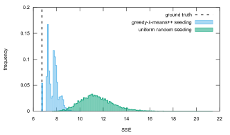
Figure 2: Histogram of the cost obtained from $10^{4}$ runs of Lloyd’s algorithm with uniform initialization and with greedy-$k$-means++ initialization, on the A3 synthetic dataset (see main text; we scaled the data uniformly to make it fit into a $\left[0,1\right]\times\text{$\left[0,1\right]$}$ square, by dividing all data entries by the overall maximum). The latter algorithm clearly finds better configurations on average, and in $5.4\%$ of the cases reaches the level of the ground truth (see the first, isolated peak on the left). The following two peaks are, roughly speaking, due to configurations with one or two “mistakes”, respectively (see fig. 3).

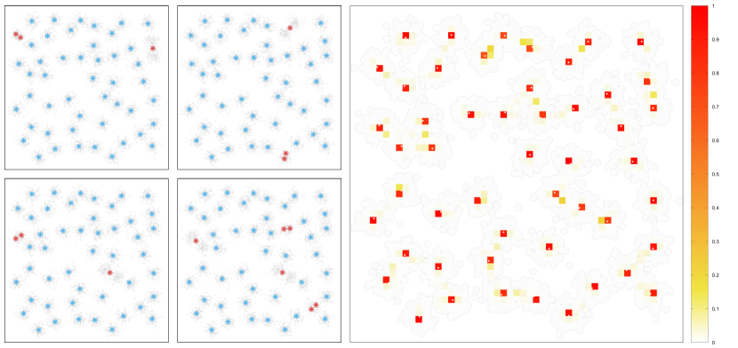
Figure 3: Left four panels. Examples of “typical” configurations found by 4 independent runs of Lloyd’s algorithm with greedy-$k$-means++ seeding, on the $2$-dimensional A3 dataset (same as for fig. 2). The data is represented in gray, and the centroids in blue, except for “mistakes” which are shown in red. The first three panels show configurations corresponding to the highest peak in the histogram of fig. 2 (one mistake each, centroid index $\mathrm{CI}=1$), while the bottom-right panel shows a configuration corresponding to the following peak (two mistakes, $\mathrm{CI}=2$). The fact that these mistakes are few and mostly independent is shown quantitatively in the right panel, which depicts a two-dimensional histogram of the distribution of the centroids found over $10^{4}$ runs by the local optimizer, same data as for fig. 2. This graph aims at showing the effect of superimposing several solutions like the ones shown in the left panels. The area (a square of size $1$) was binned in squares of size $0.02$. All of the red peaks correspond to the optimal configuration (the optimal centroids are shown as small white dots and they are indistinguishable from the ground truth at this level of detail), and they all have a value of $0.7$ or more. Outside of the optimal bins, all other bins are barely distinguishable from the white background: none of them is higher than $0.22$, meaning that no other location has a higher chance than $22\%$ of being produced in a run of the algorithm. Overall, this shows that in examples like this one the centroids of completed runs cluster extremely well around the optimal ones.

Here, we start by analyzing the results of multiple restarts on the A3 synthetic dataset from the repository of ref. [29], which is a moderately large two-dimensional dataset ($N=7500$, $D=2$) consisting of $k=50$ fairly well-distinct homogeneous clusters. The choice of this dataset is for illustrative purposes: it is designed such that optimizing the $\mathrm{SSE}$ objective leads to a near-perfect clustering, and yet finding such solution from scratch is a non-trivial task. (For this dataset, the ground truth – the centroids used for generating the data – is known, and the globally optimal configuration is indeed extremely close to it.) Furthermore, it is two-dimensional, and thus it can be easily visualized. Finally, as we shall show, it is quite easy to visually identify and understand “mistakes” in the clustering for the sub-optimal fixed points that are sufficiently close to the global optimum.

We performed $10^{4}$ runs of local optimization (Lloyd’s algorithm) on this dataset, seeding the algorithm with greedy-$k$-means++, and also as many runs with random uniform seeding (what’s commonly referred to as $k$-means) for comparison. The histogram of the costs is shown in fig. 2. It can be noted that the uniform-seeding version never reached the level of the ground truth cost. Greedy-$k$-means++ seeding on the other hand led to finding a cost comparable to that of the ground truth in $5.4\%$ of the cases. The clear gap between the ground-truth-level and the rest of the histogram allows us to informally denote the configurations in the leftmost peak as “successes”: these are all configurations that any sensible method (from visual inspection to more detailed analytical tools) would classify as near-perfect. More formally, these configurations all have a centroid index (CI), as defined in ref. [30] , of $0$ (and all other configurations, from the second peak onward, have $\mathrm{CI>}0$). With the observed percentage of success of $5.4\%$ of greedy-$k$-means++, we can easily compute (with the inverse of a geometric cumulative distribution function) that one would need about $R=54$ runs to reach a confidence level of $95\%$ of success with a simple multiple restarts strategy, and $R=83$ to reach a confidence of $99\%$.

A further inspection of fig. 2 shows that, even when unsuccessful, the algorithm has a few clearly visible peaks that are close to the optimum. These peaks correspond to situations that are depicted in the four left panels of figure 3. Overall, one can qualitatively observe that, in most runs, most centroids end up being near their optimal position, with only a few, fairly well identifiable “mistakes”. Moreover, these mistakes are mostly independent from one run to the next. This is confirmed when superimposing the final centroids obtained from different runs, shown in the right panel of figure 3, whereby we see how they form tight, dense clusters around the optimal centroids.

-B Parameters choice: The effect of varying $\Delta\beta$

$\Delta\beta$	A3		Birch1		Birch2
	time ($s$)	succ.rate	time ($s$)	succ.rate	time ($s$)	succ.rate
$0$	$0.091\pm 0.016$	$100\%$	$3.9\pm 0.3$	$100\%$	$2.2\pm 0.4$	$100\%$
$0.1$	$0.089\pm 0.014$	$100\%$	$4.0\pm 0.3$	$100\%$	$2.2\pm 0.4$	$100\%$
$1$	$0.084\pm 0.014$	$99.9\%$	$3.7\pm 0.3$	$100\%$	$2.1\pm 0.3$	$100\%$
$10$	$0.079\pm 0.012$	$97.3\%$	$3.6\pm 0.3$	$93\%$	$1.9\pm 0.2$	$100\%$

Table VI: Average and standard deviation of convergence time (in seconds), and success rate, for recombinator-kmeans on a few synthetic datasets, varying $\Delta\beta$, $1000$ samples per point for A3 and $100$ samples per point for Birch1 and Birch2.

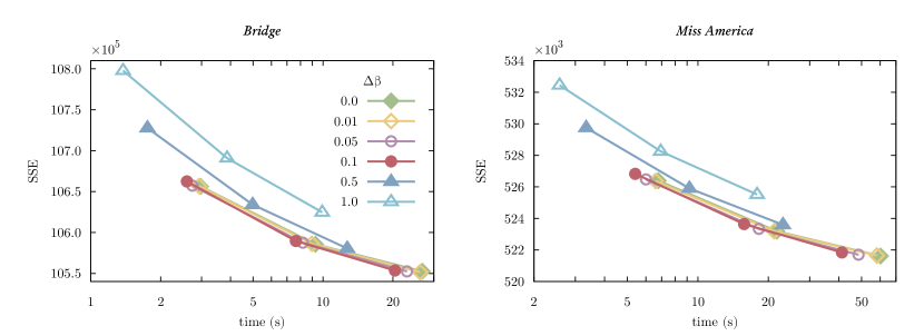
Figure 4: Results of recombinator-kmeans on two datasets, Bridge and Miss America, with different $\Delta\beta$ and varying $J$ in $\left\{5,10,20\right\}$; $500$ samples per point (average values shown, error bars omitted for clarity).

In table VI we show the average convergence time and success rate of recombinator-kmeans with $J=5$ and different $\Delta\beta$, for three synthetic datasets. This is an extension of the result shown for $\Delta\beta=0.1$ in table 2 of the main text. The $\Delta\beta=0$ case corresponds to uniform weighting. For these datasets (and similar ones with a well-defined clustering structure, like those of sec. VI.B of the main text) the performance is only mildly affected by $\Delta\beta$ in a wide range; the success rate is $100\%$ even with uniform weights and only starts to be affected at very large $\Delta\beta$ (and in those cases a larger $J$ would restore the perfect score). Indeed, in all these cases, the second batch is already very likely to contain a ground-truth-level configuration, as per the discussion in sec. 5 of the main text and sec. -A above; a third batch (or very rarely a fourth) may be required in the harder cases only to detect convergence.

The situation is less straightforward when the optimization problems are more challenging with no clear solution, as for the datasets of sec. VI.C of the main text. Figure 4 shows two examples of varying the $\Delta\beta$ parameter of recombinator-kmeans, on the Bridge and Miss America datasets. Our tests with other datasets and configurations suggest that the behavior shown is fairly well representative of challenging problems. A few exceptions manifested with very small values of $\Delta\beta$: setting $\Delta\beta=0$ effectively removes the weighting and therefore the guarantee of convergence. We have observed cases with less than 50% chance of convergence and major effects on convergence time with that setting.

From the figure we can observe that, in general, increasing $\Delta\beta$ reduces the convergence time (which is expected) but results in a greedier algorithm. On balance, the setting $\Delta\beta=0.1$ seems to be close to optimal in most cases. But the data also shows that overall the effect of $\Delta\beta$ is rather mild.

-C Parameters choice: The effect of varying $t_{\mathrm{max}}$

Figure 5: Results of recombinator-kmeans on two datasets, Bridge and Miss America, with different $t_{\mathrm{max}}$ and varying $J$ in $\left\{5,10,20\right\}$; $500$ samples per point (average values shown, error bars omitted for clarity).

The effect of the $t_{\max}$ parameter for recombinator-kmeans depends on the dataset. For the synthetic datasets of the first batch of tests, section VI.B of the main text, using $t_{\max}=10$ instead of allowing unlimited iterations has at most negligible effects, since typically Lloyd’s algorithm converges much earlier than the cutoff in those cases (when seeded with greedy-$k$-means++).

In fig. 5 we show the effect of varying $t_{\max}$ in some more challenging cases, the Bridge and Miss America datasets (see sec. VI.C of the main text). In both cases we tested $t_{\max}=2$, $10$ and unbounded. From these examples, which appear to be fairly representative, it seems that capping the iterations at $10$ can lead to some small improvements in the cost-vs-time tradeoff. This appears to be the case even though the time gains of the cutoff are diminished by the use of the technique of ref. [22] that speeds up Lloyd iterations, and which is particularly effective as the iterations progress. The setting $t_{\max}=2$, on the other hand, appears to be excessive. Overall, as for the $\Delta\beta$ parameter, the effect of varying $t_{\mathrm{max}}$ appears to be mild in a reasonably wide range.

-D Statistical significance analysis

In this section we report the results of a statistical significance analysis on the results of sec. VI.C of the main text. For each dataset, we compared the $\mathrm{SSE}$ costs of pairs of different algorithms at “corresponding” values of $J$: we compared ga-kmeans-raw with ga-kmeans++ at the same $J$; we compared recombinator-kmeans with ga-kmeans++ at values of $J$ that resulted in roughly the same convergence time (see table III of the main text); we compared the largest available $J$ of recombinator-kmeans with randswap-kmeans++.

Each comparison was performed via two different non-parametric techniques. Given two sets of costs, $\Phi_{a}$ and $\Phi_{b}$, possibly of different sizes, we aimed at testing the null hypothesis that they were originating from the same distribution. We used both a standard two-sided Wilcoxon rank-sum test (also known as Mann-Whitney U test), and a simple bootstrapping scheme, which we defined as follows. Denoting with $\bar{\Phi}_{a}$ and $\bar{\Phi}_{b}$ the means of the costs sets, we estimated the frequency, under the null hypotheses, with which their distance $\left|\bar{\Phi}_{a}-\bar{\Phi}_{b}\right|$ would be larger or equal than the one measured. For this purpose, we pooled together all the costs, $\Phi_{U}=\Phi_{a}\cup\Phi_{b}$, and repeated $n_{B}=10^{5}$ times the following procedure: we randomly reassigned the costs in $\Phi_{U}$ to two subsets with the same size as the originals, and computed the distance of their means. We then used the fraction of cases in which the distance exceeded the measured one as the $p$-value.

This comparison is adequate for the purposes of determining whether an algorithm is actually significantly better than another in terms of the cost-vs-time trade-off only when the times are very similar. This is generally the case for the recombinator vs ga++ and recombinator vs randswap++ comparisons. However for the ga-raw vs ga++ comparison this test does not adequately take into account the fact that ga-raw is generally slightly faster.

dataset	ga++ vs ga-raw			rec. vs ga++			rec. vs rs++
	$J$	$p$-value	w	$J$	$p$-value	w	$J$	$p$-value	w
Bridge	$15$	$4.8\cdot 10^{-3}$	2	$5$	$<10^{-4}$	2
	$45$	$0.73$	2	$10$	$0.34$	2
	$120$	$0.59$	2	$20$	$<10^{-4}$	1
	$351$	$0.91$	3	$40$	$<10^{-4}$	1
	$861$	$0.99$	3	$80$	$<10^{-4}$	1	$80$	$<10^{-4}$	1
House	$10$	$1.4\cdot 10^{-3}$	2	$5$	$<10^{-4}$	2
	$28$	$6.8\cdot 10^{-3}$	2	$10$	$<10^{-4}$	2
	$66$	$5\cdot 10^{-4}$	2	$20$	$0.34$	2
	$153$	$5.2\cdot 10^{-2}$	2	$40$	$0.88$	2
	$378$	$2.4\cdot 10^{-2}$	2	$80$	$0.87$	2	$80$	$<10^{-4}$	1
M. Am.	$15$	$<10^{-4}$	2	$5$	$<10^{-4}$	2
	$45$	$<10^{-4}$	2	$10$	$<10^{-4}$	2
	$120$	$<10^{-4}$	2	$20$	$<10^{-4}$	1
	$276$	$2\cdot 10^{-4}$	2	$40$	$<10^{-4}$	1
	$741$	$0.25$	2	$80$	$<10^{-4}$	1	$80$	$<10^{-4}$	1
Urb.GB	$21$	$<10^{-4}$	2	$5$	$<10^{-4}$	2
	$55$	$<10^{-4}$	2	$10$	$<10^{-4}$	1
	$136$	$<10^{-4}$	2	$20$	$<10^{-4}$	1	$20$	$<10^{-4}$	1
Olivetti	$21$	$1.3\cdot 10^{-2}$	2	$5$	$<10^{-4}$	2
	$55$	$5.2\cdot 10^{-2}$	2	$10$	$<10^{-4}$	2
	$153$	$1.1\cdot 10^{-3}$	2	$20$	$0.69$	2
	$435$	$0.11$	2	$40$	$2.4\cdot 10^{-3}$	1
	$1225$	$<10^{-4}$	2	$80$	$0.48$	2	$80$	$<10^{-4}$	1

Table VII: Significance analysis results (bootstrapping scheme). The “w” columns indicate which of the two algorithms gave the best average cost, where $1$=recombinator, 2=ga++, 3=ga-raw, 4=randswap++. The cases in which the $p$-value is smaller than $10^{-2}$ are marked in bold. We do not report precisely values smaller than $10^{-4}$ due to the limited resolution of our bootstrapping scheme. The values of $J$ in the middle column refer to the recombinator algorithm, while the corresponding value of $J$ for ga++ is that of the first column.

The results of the analysis are reported in table VII. We report only the $p$-values for the bootstrapping comparison, as they are generally slightly larger than the ones from the Wilcoxon rank-sum tests; however, the two tests are generally in excellent agreement, and they are in complete agreement about which results are significant when using a significance threshold of $10^{-2}$ (i.e., the “w” columns would look identical). The last column shows that recombinator-kmeans is significantly superior to randswap-kmeans++ in all cases. The middle column shows that ga-kmeans++ is generally superior to recombinator-kmeans at small $J$, but that at larger $J$ recombinator-kmeans catches up and, in 3 cases out of 5, ends up being significantly better. The first column shows that ga-kmeans++ gives better or equal costs than ga-kmeans-raw. Although (as mentioned above) this is measured at fixed $J$ rather than at fixed amount of time spent, visual comparison with fig. 1 of the main text shows that most of these results are sensible, except for the ones for the Bridge and Olivetti dataset in which the few detected significant results are almost certainly spurious.

References

- [1] Xindong Wu, Vipin Kumar, J Ross Quinlan, Joydeep Ghosh, Qiang Yang, Hiroshi Motoda, Geoffrey J McLachlan, Angus Ng, Bing Liu, S Yu Philip, et al. Top 10 algorithms in data mining. Knowledge and information systems, 14(1):1–37, 2008. URL: https://doi.org/10.1007/s10115-007-0114-2.
- [2] Pavel Berkhin. A survey of clustering data mining techniques. In Grouping multidimensional data, pages 25–71. Springer, 2006. URL: https://doi.org/10.1007/3-540-28349-8_2.
- [3] Stuart Lloyd. Least squares quantization in pcm. IEEE transactions on information theory, 28(2):129–137, 1982. URL: https://doi.org/10.1109/TIT.1982.1056489.
- [4] Daniel Aloise, Amit Deshpande, Pierre Hansen, and Preyas Popat. Np-hardness of euclidean sum-of-squares clustering. Machine learning, 75(2):245–248, 2009. URL: https://doi.org/10.1007/s10994-009-5103-0.
- [5] M Emre Celebi, Hassan A Kingravi, and Patricio A Vela. A comparative study of efficient initialization methods for the k-means clustering algorithm. Expert systems with applications, 40(1):200–210, 2013. URL: https://doi.org/10.1016/j.eswa.2012.07.021.
- [6] Pasi Fränti and Sami Sieranoja. How much k-means can be improved by using better initialization and repeats? Pattern Recognition, 2019. URL: https://doi.org/10.1016/j.patcog.2019.04.014.
- [7] James MacQueen. Some methods for classification and analysis of multivariate observations. In Proceedings of the fifth Berkeley symposium on mathematical statistics and probability, volume 1: statistics, volume 1, pages 281–297. Oakland, CA, USA, University of California Press, 1967. URL: https://projecteuclid.org/euclid.bsmsp/1200512992.
- [8] David Arthur and Sergei Vassilvitskii. k-means++: The advantages of careful seeding. In Proceedings of the eighteenth annual ACM-SIAM symposium on Discrete algorithms, pages 1027–1035. Society for Industrial and Applied Mathematics, 2007. URL: http://theory.stanford.edu/~sergei/papers/kMeansPP-soda.pdf.
- [9] David E Goldberg. Genetic algorithms in search, optimization and machine learning. Addison-Wesley Longman Publishing, 1989. URL: https://doi.org/10.5860/choice.27-0936.
- [10] John Henry Holland et al. Adaptation in natural and artificial systems: an introductory analysis with applications to biology, control, and artificial intelligence. MIT press, 1992. URL: https://ieeexplore.ieee.org/servlet/opac?bknumber=6267401.
- [11] John R Koza. Genetic programming as a means for programming computers by natural selection. Statistics and computing, 4(2):87–112, 1994. URL: https://doi.org/10.1007/BF00175355.
- [12] Eduardo Raul Hruschka, Ricardo JGB Campello, Alex A Freitas, et al. A survey of evolutionary algorithms for clustering. IEEE Transactions on Systems, Man, and Cybernetics, Part C (Applications and Reviews), 39(2):133–155, 2009. URL: https://doi.org/10.1109/TSMCC.2008.2007252.
- [13] Pasi Fränti. Genetic algorithm with deterministic crossover for vector quantization. Pattern Recognition Letters, 21(1):61–68, 2000. URL: https://doi.org/10.1016/S0167-8655(99)00133-6.
- [14] Pablo Moscato and Michael G Norman. A "memetic" approach for the traveling salesman problem implementation of a computational ecology for combinatorial optimization on message-passing systems. In In Proceedings of the International Conference on Parallel Computing and Transputer Applications, volume 1, pages 177–186. IOS Press, 1992. URL: http://citeseerx.ist.psu.edu/viewdoc/summary?doi=10.1.1.50.1940.
- [15] Peter Merz and Andreas Zell. Clustering gene expression profiles with memetic algorithms. In International Conference on Parallel Problem Solving from Nature, pages 811–820. Springer, 2002. URL: https://doi.org/10.1007/3-540-45712-7_78.
- [16] Tian Zhang, Raghu Ramakrishnan, and Miron Livny. Birch: an efficient data clustering method for very large databases. ACM sigmod record, 25(2):103–114, 1996. URL: https://doi.org/10.1145/235968.233324.
- [17] Guojun Gan and Michael Kwok-Po Ng. K-means clustering with outlier removal. Pattern Recognition Letters, 90:8–14, 2017. URL: https://doi.org/10.1016/j.patrec.2017.03.008.
- [18] Weiwei Liu, Xiaobo Shen, and Ivor W Tsang. Sparse embedded k-means clustering. In I. Guyon, U. V. Luxburg, S. Bengio, H. Wallach, R. Fergus, S. Vishwanathan, and R. Garnett, editors, Proceedings of the 31st International Conference on Neural Information Processing Systems, volume 30, pages 3321–3329. Curran Associates, Inc., 2017. URL: https://papers.nips.cc/paper/2017/hash/3214a6d842cc69597f9edf26df552e43-Abstract.html.
- [19] Juha Kivijärvi, Pasi Fränti, and Olli Nevalainen. Self-adaptive genetic algorithm for clustering. Journal of Heuristics, 9(2):113–129, 2003. URL: https://doi.org/10.1023/A:1022521428870.
- [20] Shigeyoshi Tsutsui and Ashish Ghosh. A study on the effect of multi-parent recombination in real coded genetic algorithms. In 1998 IEEE international conference on evolutionary computation proceedings. IEEE World Congress on Computational Intelligence (Cat. No. 98TH8360), pages 828–833. IEEE, 1998. URL: https://doi.org/10.1109/ICEC.1998.700159.
- [21] Agoston E Eiben. Multiparent recombination in evolutionary computing. In Advances in evolutionary computing, pages 175–192. Springer, 2003. URL: https://doi.org/10.1007/978-3-642-18965-4_6.
- [22] Timo Kaukoranta, P Franti, and Olli Nevalainen. Reduced comparison search for the exact gla. In Proceedings DCC’99 Data Compression Conference (Cat. No. PR00096), pages 33–41. IEEE, 1999. URL: https://doi.org/10.1109/DCC.1999.755651.
- [23] F. Pedregosa, G. Varoquaux, A. Gramfort, V. Michel, B. Thirion, O. Grisel, M. Blondel, P. Prettenhofer, R. Weiss, V. Dubourg, J. Vanderplas, A. Passos, D. Cournapeau, M. Brucher, M. Perrot, and E. Duchesnay. Scikit-learn: Machine learning in Python. Journal of Machine Learning Research, 12:2825–2830, 2011. URL: http://www.jmlr.org/papers/v12/pedregosa11a.html.
- [24] scikit-learn. URL: https://scikit-learn.org.
- [25] Code repository for recombinator--means and our implementation of GA--means. URL: https://github.com/carlobaldassi/RecombinatorKMeans.jl.
- [26] Thomas Bäck, David B Fogel, and Zbigniew Michalewicz. Evolutionary computation 1: Basic algorithms and operators. CRC press, 2018.
- [27] URL: https://www.uef.fi/web/machine-learning/software.
- [28] Pasi Fränti. Efficiency of random swap clustering. Journal of Big Data, 5(1):13, 2018. URL: https://doi.org/10.1186/s40537-018-0122-y.
- [29] Pasi Fränti and Sami Sieranoja. K-means properties on six clustering benchmark datasets. Applied Intelligence, 48(12):4743–4759, 2018. URL: http://cs.uef.fi/sipu/datasets/.
- [30] Pasi Fränti, Mohammad Rezaei, and Qinpei Zhao. Centroid index: cluster level similarity measure. Pattern Recognition, 47(9):3034–3045, 2014. URL: https://doi.org/10.1016/j.patcog.2014.03.017.
- [31] Dheeru Dua and Casey Graff. UCI machine learning repository, 2017. URL: http://archive.ics.uci.edu/ml.
- [32] URL: https://scikit-learn.org/stable/datasets/real_world.html#the-olivetti-faces-dataset.
- [33] Marina Meilă. Comparing clusterings–an information based distance. Journal of multivariate analysis, 98(5):873–895, 2007. URL: https://doi.org/10.1016/j.jmva.2006.11.013.
- [34] Olivier Bachem, Mario Lucic, Hamed Hassani, and Andreas Krause. Fast and provably good seedings for k-means. In D. D. Lee, M. Sugiyama, U. V. Luxburg, I. Guyon, and R. Garnett, editors, Advances in Neural Information Processing Systems 29, pages 55–63. Curran Associates, Inc., 2016. URL: http://papers.nips.cc/paper/6478-fast-and-provably-good-seedings-for-k-means.pdf.
- [35] Fernando G Lobo and Cláudio F Lima. A review of adaptive population sizing schemes in genetic algorithms. In Proceedings of the 7th annual workshop on Genetic and evolutionary computation, pages 228–234, 2005. URL: https://doi.org/10.1145/1102256.1102310.
- [36] Paul S Bradley and Usama M Fayyad. Refining initial points for k-means clustering. In ICML, volume 98, pages 91–99. Citeseer, 1998. URL: http://citeseerx.ist.psu.edu/viewdoc/download?doi=10.1.1.50.8528&rep=rep1&type=pdf.