First principles study of the vibronic coupling in positively charged C${}_{60}^{+}$

Abstract

Vibronic coupling parameters for C${}_{60}^{+}$ were derived via DFT calculations with hybrid B3LYP and CAM-B3LYP functional, based on which the static Jahn-Teller effect were analyzed. The global minima of adiabatic potential energy surface (APES) shows a D_5d Jahn-Teller deformation, with stabilization energies of 110 and 129 meV (with B3LYP and CAM-B3LYP respectively), which are two times larger than that in C${}_{60}^{-}$, suggesting the crucial role of the dynamical Jahn-Teller effect. Present results enable us to assess the actual situation of dynamical Jahn-Teller effect in C${}_{60}^{+}$ and excited C₆₀ in combination with the established parameters for C${}_{60}^{-}$.

I Introduction

Recent experimental confirmation of the presence of C${}_{60}^{+}$ as interstellar materials Campbell et al. (2015, 2016) renewed the interests in C₆₀ cations, and burst various spectroscopic and theoretical investigations on C${}_{60}^{+}$ and related systems Spieler et al. (2017); Yamada, Ross, and Ito (2017); Strelnikov et al. (2018); Kaiser et al. (2018); Lykhin, Ahmadvand, and Varganov (2019); Cordiner et al. (2019). It is known that C₆₀ in its charged and excited states exhibits complex Jahn-Teller (JT) effect due to its high symmetry ($I_{h}$) Chancey and O’Brien (1997); Bersuker (2006). In particular, JT effect in C${}_{60}^{+}$ is one of the most involved cases because of the five-fold degenerate highest occupied molecular orbitals (HOMOs) of C₆₀. Toward understanding JT effect in C${}_{60}^{n+}$ cations, spectroscopic Brühwiler et al. (1997); Canton et al. (2002); Kern et al. (2013) and theoretical Ceulemans and Fowler (1990); Moate et al. (1996); De Los Rios, Manini, and Tosatti (1996); Manini, Gattari, and Tosatti (2003); Lijnen and Ceulemans (2005); Hands et al. (2006a, b, 2007); Ceulemans et al. (2012) investigations have been piled up.

Realistic description of JT effect in positively charged C₆₀ relies on the combination of an adequate model and accurate enough vibronic coupling parameters. Derivations of vibronic coupling parameters have been addressed Manini et al. (2001); Saito (2002); Ramanantoanina et al. (2013), and comprehensive sets of parameters have been estimated by density functional theory (DFT) calculations at local density approximation (LDA) level Manini et al. (2001); Ramanantoanina et al. (2013). Nevertheless, in studies about C${}_{60}^{-}$, it has been shown that LDA tends to underestimate the coupling parameters Iwahara et al. (2010), while hybrid B3LYP functional is found to give closer parameters to the experimental data. Furthermore, a good agreement between B3LYP and GW approximation calculations Faber et al. (2011) supports the accuracy of hybrid functional in studies of C₆₀. Besides, one recent study showed that B3LYP with long-range interaction correction, CAM-B3LYP, could improve the accuracy of vibronic parameters in C${}_{60}^{-}$ with respect to experimental data, indicating CAM-B3LYP could give vibronic parameters much closer to the real situationHuang and Liu (2020). Therefore, it is desired to derive the coupling parameters at a better level than LDA for accurate description of C₆₀ cations.

In this work, we derived orbital vibronic coupling parameters for C${}_{60}^{+}$ via DFT calculations with both B3LYP and CAM-B3LYP hybrid functionals. These obtained vibronic coupling parameters were compared with the previous data obtained by LDA calculations. Based on these parameters, the adiabatic potential energy surface (APES) was analyzed, and the symmetry of JT deformed C${}_{60}^{+}$ as well as static JT energies were established.

II Vibronic Hamiltonian

The highest occupied molecular orbitals (HOMOs) of C₆₀ with $I_{h}$ symmetry Kroto et al. (1985) are characterized by five-fold degenerate $h_{u}$ irreducible representation. According to selection rule, these orbitals linearly couple to mass-weighted normal vibrational modes involved in the symmetric product of $h_{u}$ representation Jahn and Teller (1937):

$$[h_{u}\otimes h_{u}]=a_{g}\oplus g_{g}\oplus 2h_{g}.$$ (1)

Among them, $g_{g}$ and $h_{g}$ modes are JT active, while $a_{g}$ is not because is does not change the symmetry of molecules. Thus, taking the equilibrium structure of neutral C₆₀ as the reference, $H\otimes(a\oplus g\oplus 2h)$ JT Hamiltonian for C${}_{60}^{+}$ is expressed as Ceulemans and Fowler (1990); Chancey and O’Brien (1997); Bersuker (2006)

$$H = H_{0}+H_{\text{JT}},$$ (2)

$$H_{0} = \frac{1}{2}\left(p_{a}^{2}+\omega_{a}^{2}q_{a}^{2}\right)+V_{a}q_{a}+\sum_{\gamma=a,x,y,z}\frac{1}{2}\left(p_{g\gamma}^{2}+\omega_{g}^{2}q_{g\gamma}^{2}\right)$$ (3)

$$+ \sum_{\gamma=\theta,\epsilon,\xi,\eta,\zeta}\frac{1}{2}\left(p_{h\gamma}^{2}+\omega_{h}^{2}q_{h\gamma}^{2}\right),$$

$$H_{\text{JT}} = V_{g}\sum_{\gamma=a,x,y,z}\hat{C}_{g\gamma}q_{g\gamma}+\frac{\sqrt{5}V_{1h}}{2}\sum_{\gamma=\theta,\epsilon,\xi,\eta,\zeta}\hat{C}_{1h\gamma}q_{1h\gamma}$$ (4)

$$+ \frac{\sqrt{5}V_{2h}}{2}\sum_{\gamma=\theta,\epsilon,\xi,\eta,\zeta}\hat{C}_{2h\gamma}q_{2h\gamma}$$

where $\omega_{\Gamma}$ ($\Gamma=a_{g},g_{g},h_{g}$) are vibration frequencies, $q_{\Gamma}$ are mass-weighted normal coordinates Inui, Tanabe, and Onodera (1990), $V_{\Gamma}$ is vibronic coupling parameter for $\Gamma$ mode, and $\hat{C}_{\Gamma\gamma}$ ($\gamma$ = a, x, y, z, $\theta$, $\epsilon$, $\xi$, $\eta$, $\zeta$) are the Clebsch-Gordan coefficients, which are taken from Ref. Liu et al. (2018) and listed in Appendix A. A coefficient $\sqrt{5}/2$ is multiplied to vibronic couplings terms of $h_{g}$ modes so that JT energy becomes:

$$E_{g}^{\text{JT}}=-\frac{V_{g}^{2}}{2\omega^{2}_{g}},\quad E_{nh}^{\text{JT}}=-\frac{V_{nh}^{2}}{2\omega^{2}_{h}},\quad(n=1,2).$$ (5)

There are two vibronic couplings to one $h_{g}$ mode because $h_{g}$ representation appears twice in selection rule, Eq. (1). The basis of vibronic Hamiltonian matrices are $H_{u}$ electronic states of C${}_{60}^{+}$ in the order of $|H_{u}\theta\rangle$, $|H_{u}\epsilon\rangle$, $|H_{u}\xi\rangle$, $|H_{u}\eta\rangle$, $|H_{u}\zeta\rangle$. For $h_{g}$ and $h_{u}$ representations, $d$ orbital type basis are used, and hence, $\theta,\epsilon,\xi,\eta,\zeta$ transform as $(2z^{2}-x^{2}-y^{2})/\sqrt{6}$, $(x^{2}-y^{2})/\sqrt{2}$, $\sqrt{2}yz$, $\sqrt{2}zx$, $\sqrt{2}xy$, respectively, under rotation. Although C₆₀ has two $a_{g}$, six and eight sets of $g_{g}$ and $h_{g}$ modes, respectively, and indices distinguishing them are not explicitly written in Eq. (3) for simplicity. Phase factors of mass-weighted normal modes are the same as those in the Supplemental Materials of Ref. Liu et al. (2018). Since the equilibrium geometry of C₆₀ is chosen as the reference structure of C${}_{60}^{+}$, vibronic coupling parameters of totally symmetric modes are also nonzero. JT energy by totally symmetric deformation is

$$E_{a} = -\frac{V_{a}^{2}}{2\omega_{a}^{2}}.$$ (6)

In many other literatures, like the work of A. CeulemansCeulemans and Fowler (1990), linear combinations of real $d$-type functions, $d_{z^{2}},d_{x^{2}-y^{2}}$, are used, which could be transformed into irreducible representation in this work by

$$q_{\theta}=\sqrt{\frac{5}{8}}Q_{\theta}+\sqrt{\frac{3}{8}}Q_{\epsilon},\quad q_{\epsilon}=\sqrt{\frac{3}{8}}Q_{\theta}-\sqrt{\frac{5}{8}}Q_{\epsilon},$$ (7)

where $Q_{\theta}$ and $Q_{\epsilon}$ are normal coordinates in Ref. Ceulemans and Fowler (1990), while $q_{\theta}$ and $q_{\epsilon}$ are normal coordinates in this work, resulting in the relation between coupling parameters $V_{1h}$ and $V_{2h}$ in this work and $F_{Hb}$ and $F_{Ha}$ defined in Ref. Ceulemans and Fowler, 1990:

$$V_{1h}=\frac{F_{Hb}}{4\sqrt{5}},\quad V_{2h}=\frac{F_{Ha}}{12\sqrt{5}}.$$ (8)

The modification introduced here is to treat the JT Hamiltonian in a framework consistent to the standard one in C${}_{60}^{-}$ Chancey and O’Brien (1997).

III Results

III.1 Orbital vibronic coupling parameters

Vibronic coupling constants of C₆₀ have been most intensively investigated in the case of C${}_{60}^{-}$, and coupling constants have been derived by various methods. By definition, vibronic coupling parameters for JT active $h_{g}$ modes, $V_{h_{g}}^{-}$, can be derived by Iwahara et al. (2010)

$$V_{h_{g}}^{-} = -\left.\frac{\partial E_{z}^{-}(\textbf{q}_{h_{g}})}{\partial q_{h_{g}\theta}}\right|_{\textbf{q}_{h_{g}}=\textbf{0}},$$ (9)

where $E_{z}^{-}(\textbf{q}_{h_{g}})=\langle T_{1u}z|\hat{H}^{-}|T_{1u}z\rangle$, $|T_{1u}z\rangle$ is $t_{1u}z$ electronic state of C${}_{60}^{-}$, $\hat{H}^{-}$ is Hamiltonian for C${}_{60}^{-}$, and $\textbf{q}_{h_{g}}=\textbf{0}$ indicates equilibrium structure of C₆₀. Because of symmetry, contributions from occupied orbitals are zero, and only partially filled $t_{1u}$ orbital level contribute to vibronic couplings. In the case of C${}_{60}^{-}$, the nature of $t_{1u}$ orbitals do not differ from that of neutral C₆₀: although $t_{1u}$ orbitals are mixed with the other $t_{1u}$ orbitals, the mixing is very small due to high symmetry, and orbitals are separated from each other by large orbital energy gaps. Consequently, gradients of total energy can be approximated by those of orbital energy levels with respect to normal modes of neutral C₆₀. Indeed, in the case of C${}_{60}^{-}$, these two approaches give very close results Laflamme Janssen et al. (2010); Iwahara et al. (2010); Faber et al. (2011); Liu et al. (2018).

Similar situation is expected in C${}_{60}^{+}$: the nature of the $h_{u}$ orbital does not change by adding one hole to the same molecular structure. Thus, orbital vibronic coupling parameters of neutral C₆₀ can be used to express vibronic coupling parameters of C${}_{60}^{+}$. Since C${}_{60}^{+}$ has one hole in $h_{u}$ HOMOs, it is convenient to perform particle-hole transformation Fetter and Walecka (2003), under which, the sign of orbital vibronic coupling parameter for one electron in HOMOs of C₆₀ should be inverted for that in the case of one hole in HOMOs. Therefore,

$$V_{\Gamma}=-v_{\Gamma},$$ (10)

where $v_{\Gamma}$ is one orbital vibronic coupling parameter for C₆₀ and $V_{\Gamma}$ is the parameter for C${}_{60}^{+}$.

Orbital vibronic coupling parameters were calculated using frozen-phonon approach. Orbital energy levels of distorted C₆₀ are fitted to the eigenvalues of JT Hamiltonian matrix (Eq. (4)). In the present case, ${h_{g}(\mu)\epsilon}$ and ${g_{g}(\mu)a}$ deformations are used because diagonalizing the model Hamiltonian is easier. For DFT calculations, a triple-zeta basis set [6-311G(d)] was employed for both B3LYP and CAM-B3LYP functionals within Gaussian Frisch et al. (2016). Some fittings are shown in Fig. 1 (see Supplemental Materials for other fittings). Black points indicate DFT levels originating from HOMOs, with gray lines for energy level calculated from model Hamiltonian. Derived orbital vibronic coupling parameters are shown in Table 1. From this table, JT stabilization energies for different JT active modes are improved about 30 % with CAM-B3LYP compared with these with B3LYP. One should note that there is almost no nonlinear splitting due to vibronic effect in HOMO levels, indicating weak quadratic or higher vibronic couplings as in the case of C${}_{60}^{-}$ Liu et al. (2018). This guarantees the validity of linear vibronic model (Eq. (3)) for the description of JT effect of C₆₀ cations.

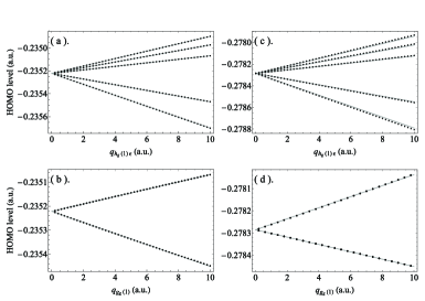
Figure 1: The JT splitting of the HOMO levels with respect to $q_{h_{g}(1)\epsilon}$ ((a) and (c)) and $q_{g_{g}(1)a}$ ((b) and (d)) deformations (in atomic unit). (a) and (b) are calculated with B3LYP functional, while (c) and (d) are with CAM-B3LYP functional. The black points and gray lines indicate the DFT values and model energy, respectively.

Table 1: The frequencies $\omega_{\Gamma}$ (cm^-1), orbital vibronic coupling parameters $v_{\Gamma}$ (10^-4 a.u.), and stabilization energies $E_{\Gamma}$ (meV) for the $a_{g}$, $g_{g}$, and $h_{g}$ modes. The data calculated with B3LYP for LUMOs are taken from Ref. Liu et al. (2018). $g_{\Gamma}=V_{\Gamma}/\sqrt{\hslash\omega_{\Gamma}^{3}}$ is dimensionless vibronic coupling parameter.

	B3LYP							CAM-B3LYP
$\mu$	$\omega_{\Gamma}$	$v_{\Gamma}$		$g_{\Gamma}$		$E_{\Gamma}$		$\omega_{\Gamma}$	$v_{\Gamma}$		$g_{\Gamma}$		$E_{\Gamma}$
		1	2	1	2	1	2		1	2	1	2	1	2
HOMO
$a_{g1}$	497	$-0.121$		$-0.112$		0.389		506	$-0.118$		$-0.106$		0.355
$a_{g2}$	1498	1.040		0.184		3.159		1527	1.369		0.236		5.268
$g_{g1}$	481	$-0.375$		$-0.366$		3.984		502	$-0.405$		$-0.370$		4.265
$g_{g2}$	584	$-0.101$		$-0.074$		0.196		586	$-0.207$		$-0.150$		0.815
$g_{g3}$	768	0.923		0.446		9.466		787	1.083		0.504		12.400
$g_{g4}$	1092	$-1.281$		$-0.365$		9.019		1092	$-1.583$		$-0.451$		13.781
$g_{g5}$	1335	0.541		0.114		1.076		1356	0.739		0.152		1.947
$g_{g6}$	1540	1.477		0.251		6.029		1576	1.571		0.258		6.509
$h_{g1}$	266	0.690	$-0.080$	1.635	$-0.190$	44.099	0.593	271	0.727	$-0.090$	1.674	$-0.206$	47.120	0.714
$h_{g2}$	439	$-0.508$	$-0.290$	$-0.568$	$-0.324$	8.776	2.860	450	$-0.558$	$-0.363$	$-0.601$	$-0.391$	10.063	4.269
$h_{g3}$	726	$-0.043$	0.977	$-0.023$	0.514	0.023	11.869	745	$-0.061$	1.053	$-0.031$	0.532	0.043	13.086
$h_{g4}$	786	0.923	$-0.059$	0.431	$-0.027$	9.038	0.037	802	0.930	$-0.139$	0.421	$-0.063$	8.821	0.198
$h_{g5}$	1125	$-0.101$	$-0.495$	$-0.028$	$-0.135$	0.053	1.269	1148	$-0.074$	$-0.565$	$-0.020$	$-0.150$	0.028	1.591
$h_{g6}$	1269	0.965	0.272	0.220	0.062	3.790	0.301	1300	0.986	0.025	0.216	0.005	3.768	0.002
$h_{g7}$	1443	2.860	1.487	0.537	0.279	25.745	6.960	1480	3.425	2.010	0.618	0.363	35.072	12.081
$h_{g8}$	1607	2.721	$-1.542$	0.434	$-0.246$	18.790	6.034	1663	3.217	$-1.701$	0.488	$-0.258$	24.523	6.854
LUMO
$a_{g1}$	497	$-0.264$		$-0.245$		1.849		506	$-0.253$		$-0.228$		1.629
$a_{g2}$	1498	$-2.380$		$-0.422$		16.543		1527	$-2.921$		$-0.503$		23.971
$h_{g1}$	266	0.192		0.455		3.415		271	0.209		0.481		3.884
$h_{g2}$	439	0.450		0.503		6.886		450	0.456		0.491		6.735
$h_{g3}$	726	0.754		0.396		7.069		745	0.849		0.429		8.512
$h_{g4}$	786	0.554		0.259		3.256		802	0.575		0.260		3.367
$h_{g5}$	1125	0.766		0.209		3.038		1148	0.827		0.219		3.402
$h_{g6}$	1269	0.578		0.132		1.360		1300	0.513		0.113		1.019
$h_{g7}$	1443	2.099		0.394		13.867		1480	2.553		0.461		19.492
$h_{g8}$	1607	2.043		0.326		10.592		1663	2.325		0.352		12.808

III.2 Static Jahn-Teller effect

Vibronic coupling lifts degeneracy with the deformation keeping one of the highest subgroup symmetries Liehr (1963), resulting in six $D_{5d}$ and ten $D_{3d}$ minima Ceulemans and Fowler (1990), as there are six $C_{5}$ and ten $C_{3}$ axes in C₆₀. Thus, based on present basis, using symmetry adapted deformations Hands et al. (2006b), deformations for $D_{5d}$ and $D_{3d}$ minima are expressed by

$${\textbf{q}}_{h_{g}}^{D_{5d}} = q_{h_{g}}\left(\frac{\phi^{2}}{2\sqrt{5}},\frac{\phi^{-1}}{2}\sqrt{\frac{3}{5}},0,\sqrt{\frac{3}{5}},0\right),$$

$${\textbf{q}}_{g_{g}}^{D_{5d}} = q_{g_{g}}\left(0,0,0,0\right),$$ (11)

and

$${\textbf{q}}_{h_{g}}^{D_{3d}} = q_{h_{g}}\left(-\frac{\phi^{-1}}{2},\frac{\phi^{2}}{2\sqrt{3}},0,\frac{1}{\sqrt{3}},0\right),$$

$${\textbf{q}}_{g_{g}}^{D_{3d}} = q_{g_{g}}\left(\frac{1}{\sqrt{6}},0,-\sqrt{\frac{5}{6}},0\right),$$ (12)

respectivelyLiu et al. (2018). Substituting these symmetrized deformations, Eqs. (III.2) and (III.2), into potential terms of model Hamiltonian (kinetic energy term is ignored), and then diagonalizing model Hamiltonian, we obtain the lowest adiabatic potential energies as

$$U^{D_{5d}} = \frac{1}{2}\omega^{2}_{h}q^{2}_{h}+V_{1h}q_{h},$$

$$U^{D_{3d}} = \frac{1}{2}\omega^{2}_{g}q^{2}_{g}+\frac{1}{2}\omega^{2}_{h}q^{2}_{h}+\frac{1}{3}\left(2V_{g}q_{g}+\sqrt{5}V_{2h}q_{h}\right),$$ (13)

for $D_{5d}$ and $D_{3d}$ deformations, respectively. Furthermore, these global minima energies could be expressed in terms of stabilization energies (Eq. (5)), asCeulemans and Fowler (1990)

$$E_{\text{JT}}^{D_{5d}} = -E_{1h}^{\text{JT}},$$

$$E_{\text{JT}}^{D_{3d}} = -\frac{1}{9}\left(4E_{g}^{\text{JT}}+5E_{2h}^{\text{JT}}\right).$$ (14)

JT stabilization energies of C${}_{60}^{+}$ are obtained using these equations and the calculated vibronic coupling parameters. When treating C${}_{60}^{+}$, we have to sum up contributions from all $g_{g}$ and $h_{g}$ modes. Manini et al. also have derived vibronic coupling parameters and JT stabilization energies in the same way with LDA. Manini et al. (2001) Besides, there is always the stabilization due to the totally symmetric modes (Eq. (6)).

JT stabilization energies of C${}_{60}^{+}$ have been calculated with different methods with various functionals. These methodologies to derive JT energies are classified into four. We denote the present method (I). In the second method, JT stabilization energy is directly obtained from the energy difference between high- and low-symmetric structures. This method was employed by Lykhin et al. Lykhin, Ahmadvand, and Varganov (2019) with B3LYP. The third and the fourth methods, (III) and (IV), are called interaction mode approach Khlopin, Polinger, and Bersuker (1978); Bersuker and Polinger (1989) and intrinsic distortion path approach Bruyndonckx et al. (1997); Zlatar, Schläpfer, and Daul (2009); Zlatar et al. (2010); Zlatar and Gruden (2019), respectively. In both methods, vibronic coupling parameters or JT energies are extracted from optimized geometry with each subgroup of $I_{h}$. The interaction mode induces deformation along JT minima from high-symmetric coordinates and is expressed by a linear combination of normal modes of high-symmetric C₆₀. The coefficients of the linear combinations contain the information of the vibronic coupling. By expanding the difference of JT deformed and high-symmetry geometries, $\Delta\textbf{R}_{\text{JT}}$, with the eigen modes of mass-weighted normal modes $\textbf{e}_{i}$ Inui, Tanabe, and Onodera (1990) at high-symmetry structure as

$$\frac{V_{i}}{\omega_{i}^{2}}=c_{i}\sqrt{M}\Delta\textbf{R}_{\text{JT}}.\textbf{e}_{i},$$ (15)

the vibronic coupling parameters $V_{i}$ could be obained. The frequencies $\omega_{i}$ are obtained from first principles calculations and $M$ is mass of carbon, and the coefficients $c_{i}$ depend on the structure of the JT interaction matrix. This approach was used in Refs. Ramanantoanina et al. (2013); Muya et al. (2013). On the other hand, within the intrinsic distortion path analysis, the high-symmetric structure is expressed by the linear combination of the eigen vectors from low-symmetric structure. Combining the vibronic coupling parameters derived from the deformation, $V^{\prime}_{i}$, and the frequencies at the low-symmetric structure, $\omega^{\prime}_{i}$, the JT energy could be written as $E_{\text{JT}}=\sum_{i}V_{i}^{\prime 2}/(2\omega_{i}^{\prime 2})$. The last method was applied to C${}_{60}^{+}$ in Ref. Ramanantoanina et al. (2013).

JT stabilization energies in this work, as well as those from previous studies, are shown in Table 2, from which we could see that CAM-B3LYP could enhance JT stabilization energies for $D_{5d}$ and $D_{3d}$ minima by 17% and 30% respectively compared to that with B3LYP. And JT stabilization energies obtained with both B3LYP and CAM-B3LYP are larger than those from LDA or PBE-related functionals. In particular, data calculated with LDA from Manini et al.,Manini et al. (2001) is only about 60 % of the present data. The underestimation of JT energy by LDA method is consistent with the situation in C${}_{60}^{-}$ Iwahara et al. (2010). However, since with LDA methods (II) and (III) give similar data as the one by method (I), Manini et al. (2001) the difference of these methods would not be the origin of discrepancies seen in B3LYP data. Thus, a possible reason is that the deformed geometry with B3LYP functional in Ref. Ramanantoanina et al. (2013) is the one at a local minima. For B3LYP, Ref. Lykhin, Ahmadvand, and Varganov (2019) and present work give much close results, whereas the former is larger than the latter by 11 meV. So such a difference is expected to come from that JT stabilization energies contributed by totally symmetric modes, Eq. (6), are included in Ref. Lykhin, Ahmadvand, and Varganov (2019). However, JT stabilization energy contributed from $a_{g}$ modes in this work is about 3.5 meV (Table 1), which is still smaller than 11 meV. The underestimation of vibronic coupling of totally symmetric modes may come from the lack of contributions from occupied orbitals and change of frequencies. In general, only the partially filled frontier orbitals contribute to the vibronic coupling to the JT modes due to the symmetry Sato, Tokunaga, and Tanaka (2006), whereas all occupied orbitals do contribute to vibronic coupling to the totally symmetric modes Sato, Tokunaga, and Tanaka (2008). Indeed, in the case of a planar molecule, picene, orbital vibronic coupling parameters for totally symmetric modes differ by 10-20 % from those obtained by fitting the gradients of total system energy Sato, Iwahara, and Tanaka (2012). Frequencies can be changed due to the removal of electron by 5-15 % Matsuda et al. (2018). Another possible origin of this discrepancy is nonlinear vibronic coupling, however, such coupling is much weaker than linear vibronic coupling as in the case of C₆₀ anions Liu et al. (2018).

Table 2: Jahn-Teller energies of C${}_{60}^{+}$ (meV) for $D_{5d}$ and $D_{3d}$ minima of the APES, respectively.

Functional	Method	$D_{5d}$	$D_{3d}$	Ref
B3LYP	(I)	110	30	Present
CAM-B3LYP	(I)	129	39	Present
LDA	(I)	69	22	Manini et al. (2001)
B3LYP	(II)	121	-	Lykhin, Ahmadvand, and Varganov (2019)
LDA	(III)	74	27	Ramanantoanina et al. (2013)
OPBE	(III)	74	28	Ramanantoanina et al. (2013)
B3LYP	(III)	80	32	Ramanantoanina et al. (2013)
PBE	(III)	74	28	Muya et al. (2013)
LDA	(IV)	72	20	Ramanantoanina et al. (2013)
OPBE	(IV)	74	21	Ramanantoanina et al. (2013)
B3LYP	(IV)	94	25	Ramanantoanina et al. (2013)

Besides these works, we note that Kern et al Kern et al. (2013) have optimized the structure to simulate infrared (IR) absorption spectrum with BP86 functional, but JT energy was not derived.

IV Discussion

To fully reveal the molecular nature of C${}_{60}^{+}$, non-adiabatic dynamical Jahn-Teller effect is crucial. The most straightforward way would be exact diagonalizing the molecular Hamiltonian, which fully quantizes both nuclear and electronic coordinates, nevertheless, it is not practical. To partly overcome this difficulty, combining Jahn-Teller model Hamiltonian (3) with accurate enough vibronic coupling parameters is indispensable to derive low-energy states.

Vibronic coupling parameters of C${}_{60}^{+}$ have been derived by using DFT calculations with LDA Manini et al. (2001); Ramanantoanina et al. (2013) and B3LYP Saito (2002) functionals. As discussed in Sec. II, model Hamiltonian is described by one vibronic coupling parameter for each $a_{g}$ and $g_{g}$ mode, and two parameters for each $h_{g}$ mode. Both parameters for the $h_{g}$ modes, $V_{1h}$ and $V_{2h}$, have been derived only in Ref. Manini et al. (2001) and Ref. Ramanantoanina et al. (2013), while they have not in Ref. Saito (2002). Ramanantoanina et al. Ramanantoanina et al. (2013) shows that the magnitudes of derived coupling parameters obtained from the gradient of HOMO levels Manini et al. (2001) and those from adiabatic potential energy surface agree well with each other, which has been also seen in C${}_{60}^{-}$ Iwahara et al. (2010); Laflamme Janssen et al. (2010); Liu et al. (2018). Thus, the present orbital vibronic coupling parameters derived from C₆₀ must be close to the parameters for C${}_{60}^{+}$ derived based on the definition.

The accuracy of LDA data have been discussed Ramanantoanina et al. (2013); Ponzellini (2014) based on the comparison between experimental photoelectron spectra (PES) Canton et al. (2002) and those from numerical simulation Manini, Gattari, and Tosatti (2003). Indeed, PES is very useful to establish vibronic coupling parameters, whereas the simulation of PES requires high accuracy both in theoretical simulation and experiments. In the case of C${}_{60}^{-}$, vibronic coupling parameters derived from broad PES at high-temperature Gunnarsson et al. (1995) have been proved to be overestimated by the simulation of high-resolution PES spectra Iwahara et al. (2010). Furthermore, it was also found that the error bar of vibronic coupling parameters derived from broad PES is very large Iwahara et al. (2010). Thus, the derivation of accurate coupling parameters is only possible if we have high-resolution PES spectra measured at low-temperature Wang, Woo, and Wang (2005); Huang et al. (2014). In the case of C${}_{60}^{+}$, as pointed out by Manini et al. Manini, Gattari, and Tosatti (2003), experimental PES is broad and fine structure of low-energy region due to vibronic coupling is completely smeared out, which prevents the direct comparison between theory and experiment. Moreover, in the case of PES of C${}_{60}^{+}$, theoretical ratio of the second strongest peak to the strongest one is smaller than those of experimental data, implying the underestimation of vibronic coupling by LDA. From this point, the present data larger than the LDA data by 40 % would give better agreement.

The quality of B3LYP calculations has been checked in C₆₀ anions by comparing theoretical and experimental data in previous studies. Besides the good agreement between coupling parameters from B3LYP calculations and high-resolution PES Iwahara et al. (2010), the good quality of B3LYP calculations also has been confirmed from Néel temperature Iwahara and Chibotaru (2013), spin gap Liu, Iwahara, and Chibotaru (2018), and the explanation for the origin of temperature evolution of infrared spectra Matsuda et al. (2018) in Mott-insulating Cs₃C₆₀ using the same vibronic coupling parameters. Furthermore, vibronic coupling parameters from B3LYP calculations tend to give good description of inelastic electron tunneling spectra of other organic molecule Shizu, Sato, and Tanaka (2010). All these facts show that B3LYP values are closer to the reality in C${}_{60}^{+}$, but there still a mismatch when compared with experimental data. The application of CAM-B3LYP could eliminate such mismatch of vibronic parameters in fullerene system, as shown in recent study of C${}_{60}^{-}$Huang and Liu (2020).

Although the derivation of vibronic coupling parameters is the first step toward full description of the molecular states of C${}_{60}^{+}$, we believe this is a crucial step. Once calculations of accurate enough vibronic states become possible, it is possible to interpret various spectra such as scanning tunneling measurements of C₆₀ Frederiksen et al. (2008), inverse PES Große et al. (2017) and angle resolved PES Latzke et al. (2019) to mention a few. Furthermore, present coupling parameters are derived based on the well-defined phase factor of normal modes which has been also used for orbital coupling parameters of LUMO Liu et al. (2018) and next LUMO Huang and Liu (2020). Therefore, by combining present coupling parameters with them, it is also possible to address complex vibronic problems of excited C₆₀ Qiu, Chibotaru, and Ceulemans (2001), and also to analyze e.g. luminescence spectra Akimoto and Kan’no (2002) and relaxation process and thermally activated delayed luminescence Stepanov et al. (2002).

V Conclusions

In this work, orbital vibronic coupling parameters for $h_{u}$ HOMO level of C₆₀ are derived using both B3LYP and CAM-B3LYP hybrid functional. We believe that these vibronic coupling parameters are high accurate and close to the real situation. With these obtained coupling parameters, JT stabilization energies of C${}_{60}^{+}$ are calculated, and JT structure at the minima of APES is confirmed to be $D_{5d}$, with the stablization energy 110 meV and 129 meV calculated with B3LYP and CAM-B3LYP, respectively. JT stabilization energies in C${}_{60}^{+}$ are about two times larger than that in C${}_{60}^{-}$, suggesting the crucial role of the dynamical JT effect to reveal the actual situation of C${}_{60}^{+}$.

Present coupling parameters have been derived within the same framework used for our studies on ground and excited C${}_{60}^{-}$. Thus, combining present data with that from other works, it is also possible to analyze the vibronic problems of excited C₆₀.

conflict of interest

There are no conflicts to declare.

VI appendix

VI.1 Clebsch-Gordan coefficients: $\hat{C}_{\Gamma\gamma}$

For the derivation of the vibronic Hamiltonian, the Clebsch-Gordan coefficients, $\hat{C}_{\Gamma\gamma}$ are taken from Ref. Liu et al. (2018), and listed below, in which $\phi=(1+\sqrt{5})/2$, $\Gamma$ = g, 1h, 2h, and $\gamma$ = a, x, y, z, $\theta$, $\epsilon$, $\xi$, $\eta$, $\zeta$.

$$\hat{C}_{ga}=\begin{pmatrix}\frac{1}{2}\sqrt{\frac{3}{2}}&0&0&0&0\\ 0&\frac{1}{2}\sqrt{\frac{3}{2}}&0&0&0\\ 0&0&-\frac{1}{\sqrt{6}}&0&0\\ 0&0&0&-\frac{1}{\sqrt{6}}&0\\ 0&0&0&0&-\frac{1}{\sqrt{6}}\end{pmatrix}$$ (16)

$$\hat{C}_{gx}=\begin{pmatrix}0&0&-\frac{\phi}{4}\sqrt{\frac{5}{2}}&0&0\\ 0&0&\frac{\phi^{-2}}{4}\sqrt{\frac{5}{6}}&0&0\\ -\frac{\phi}{4}\sqrt{\frac{5}{2}}&\frac{\phi^{-2}}{4}\sqrt{\frac{5}{6}}&0&0&0\\ 0&0&0&0&\frac{1}{2}\sqrt{\frac{5}{6}}\\ 0&0&0&\frac{1}{2}\sqrt{\frac{5}{6}}&0\end{pmatrix}$$ (17)

$$\hat{C}_{gy}=\begin{pmatrix}0&0&0&\frac{\phi^{-1}}{4}\sqrt{\frac{5}{2}}&0\\ 0&0&0&-\frac{\phi^{2}}{4}\sqrt{\frac{5}{6}}&0\\ 0&0&0&0&\frac{1}{2}\sqrt{\frac{5}{6}}\\ \frac{\phi^{-1}}{4}\sqrt{\frac{5}{2}}&-\frac{\phi^{2}}{4}\sqrt{\frac{5}{6}}&0&0&0\\ 0&0&\frac{1}{2}\sqrt{\frac{5}{6}}&0&0\end{pmatrix}$$ (18)

$$\hat{C}_{gz}=\begin{pmatrix}0&0&0&0&\frac{1}{4}\sqrt{\frac{5}{2}}\\ 0&0&0&0&\frac{5}{4\sqrt{6}}\\ 0&0&0&\frac{1}{2}\sqrt{\frac{5}{6}}&0\\ 0&0&\frac{1}{2}\sqrt{\frac{5}{6}}&0&0\\ \frac{1}{4}\sqrt{\frac{5}{2}}&\frac{5}{4\sqrt{6}}&0&0&0\end{pmatrix}$$ (19)

$$\hat{C}_{1h\theta}=\begin{pmatrix}\frac{\sqrt{5}}{16}&\frac{3\sqrt{3}}{16}&0&0&0\\ \frac{3\sqrt{3}}{16}&-\frac{\sqrt{5}}{16}&0&0&0\\ 0&0&-\frac{\phi^{-2}}{4}&0&0\\ 0&0&0&\frac{\phi^{2}}{4}&0\\ 0&0&0&0&-\frac{\sqrt{5}}{4}\end{pmatrix}$$ (20)

$$\hat{C}_{1h\epsilon}=\begin{pmatrix}\frac{3\sqrt{3}}{16}&-\frac{\sqrt{5}}{16}&0&0&0\\ -\frac{\sqrt{5}}{16}&-\frac{3\sqrt{3}}{16}&0&0&0\\ 0&0&-\frac{\sqrt{3}\phi}{4}&0&0\\ 0&0&0&\frac{\sqrt{3}\phi^{-1}}{4}&0\\ 0&0&0&0&\frac{\sqrt{3}}{4}\end{pmatrix}$$ (21)

$$\hat{C}_{1h\xi}=\begin{pmatrix}0&0&-\frac{\phi^{-2}}{4}&0&0\\ 0&0&-\frac{\sqrt{3}\phi}{4}&0&0\\ -\frac{\phi^{-2}}{4}&-\frac{\sqrt{3}\phi}{4}&0&0&0\\ 0&0&0&0&0\\ 0&0&0&0&0\end{pmatrix}$$ (22)

$$\hat{C}_{1h\eta}=\begin{pmatrix}0&0&0&\frac{\phi^{2}}{4}&0\\ 0&0&0&\frac{\sqrt{3}\phi^{-1}}{4}&0\\ 0&0&0&0&0\\ \frac{\phi^{2}}{4}&\frac{\sqrt{3}\phi^{-1}}{4}&0&0&0\\ 0&0&0&0&0\end{pmatrix}$$ (23)

$$\hat{C}_{1h\zeta}=\begin{pmatrix}0&0&0&0&-\frac{\sqrt{5}}{4}\\ 0&0&0&0&\frac{\sqrt{3}}{4}\\ 0&0&0&0&0\\ 0&0&0&0&0\\ -\frac{\sqrt{5}}{4}&\frac{\sqrt{3}}{4}&0&0&0\end{pmatrix}$$ (24)

$$\hat{C}_{2h\theta}=\begin{pmatrix}\frac{9}{16}&-\frac{\sqrt{15}}{16}&0&0&0\\ -\frac{\sqrt{15}}{16}&-\frac{9}{16}&0&0&0\\ 0&0&\frac{\phi}{4}&0&0\\ 0&0&0&-\frac{\phi^{-1}}{4}&0\\ 0&0&0&0&-\frac{1}{4}\end{pmatrix}$$ (25)

$$\hat{C}_{2h\epsilon}=\begin{pmatrix}-\frac{\sqrt{15}}{16}&-\frac{9}{16}&0&0&0\\ -\frac{9}{16}&\frac{\sqrt{15}}{16}&0&0&0\\ 0&0&-\frac{\phi^{-2}}{4\sqrt{3}}&0&0\\ 0&0&0&\frac{\phi^{2}}{4\sqrt{3}}&0\\ 0&0&0&0&-\frac{1}{4}\sqrt{\frac{5}{3}}\end{pmatrix}$$ (26)

$$\hat{C}_{2h\xi}=\begin{pmatrix}0&0&\frac{\phi}{4}&0&0\\ 0&0&-\frac{\phi^{-2}}{4\sqrt{3}}&0&0\\ \frac{\phi}{4}&-\frac{\phi^{-2}}{4\sqrt{3}}&0&0&0\\ 0&0&0&0&\frac{1}{\sqrt{3}}\\ 0&0&0&\frac{1}{\sqrt{3}}&0\end{pmatrix}$$ (27)

$$\hat{C}_{2h\eta}=\begin{pmatrix}0&0&0&-\frac{\phi^{-1}}{4}&0\\ 0&0&0&\frac{\phi^{2}}{4\sqrt{3}}&0\\ 0&0&0&0&\frac{1}{\sqrt{3}}\\ -\frac{\phi^{-1}}{4}&\frac{\phi^{2}}{4\sqrt{3}}&0&0&0\\ 0&0&\frac{1}{\sqrt{3}}&0&0\end{pmatrix}$$ (28)

$$\hat{C}_{2h\zeta}=\begin{pmatrix}0&0&0&0&-\frac{1}{4}\\ 0&0&0&0&-\frac{1}{4}\sqrt{\frac{5}{3}}\\ 0&0&0&\frac{1}{\sqrt{3}}&0\\ 0&0&\frac{1}{\sqrt{3}}&0&0\\ -\frac{1}{4}&-\frac{1}{4}\sqrt{\frac{5}{3}}&0&0&0\end{pmatrix}$$ (29)

Supplemental Materials contain the JT splitting of the HOMO levels with respect to $q_{h\epsilon}$ and $q_{ga}$deformations.

VII JT splitting of the HOMO levels

There are eight $q_{h\epsilon}$ and six $q_{ga}$ deformations, which are distinguished by the subindex, as $q_{h(1)\epsilon}$ corresponding to the first $q_{h\epsilon}$ deformation.

The DFT data with B3LYP hybrid functional and the defination of the phase factors of the normal modes are taken from Ref. Liu et al. (2018). The fitting for of the DFT HOMO levels to the model hamiltonian for $q_{h_{g}(i)\epsilon},~{}i=2,3,4,5,6,7,8$ are shown in Fig. 2, 3, 4, 5, 6, 7 and 8, while $q_{g_{g}(i)},~{}i=2,3,4,5,6$ are shown in Fig. 9, 10, 11, 12, and 13.

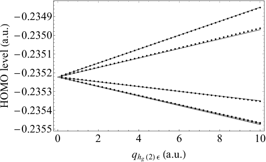
Figure 2: The JT splitting of the HOMO levels calculated by B3LYP with respect to $q_{h_{g}(2)\epsilon}$ deformation (in atomic unit). The black points and gray lines indicate the DFT values and model energy, respectively.

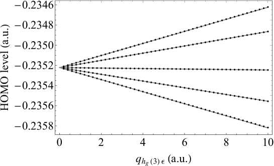
Figure 3: The JT splitting of the HOMO levels calculated by B3LYP with respect to $q_{h_{g}(3)\epsilon}$ deformation (in atomic unit). The black points and gray lines indicate the DFT values and model energy, respectively.

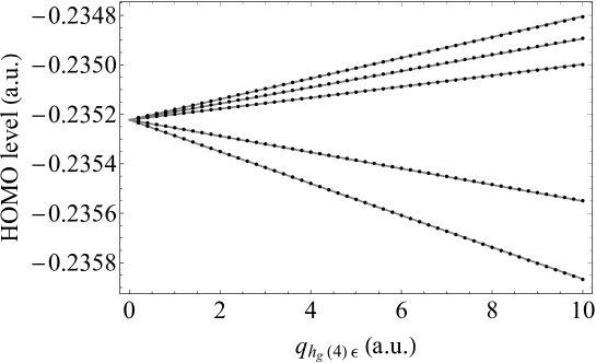
Figure 4: The JT splitting of the HOMO levels calculated by B3LYP with respect to $q_{h_{g}(4)\epsilon}$ deformation (in atomic unit). The black points and gray lines indicate the DFT values and model energy, respectively.

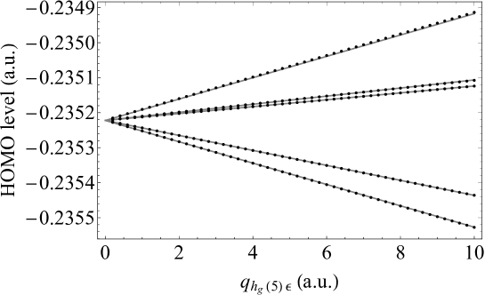
Figure 5: The JT splitting of the HOMO levels calculated by B3LYP with respect to $q_{h_{g}(5)\epsilon}$ deformation (in atomic unit). The black points and gray lines indicate the DFT values and model energy, respectively.

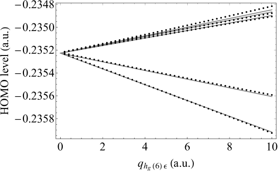
Figure 6: The JT splitting of the HOMO levels calculated by B3LYP with respect to $q_{h_{g}(6)\epsilon}$ deformation (in atomic unit). The black points and gray lines indicate the DFT values and model energy, respectively.

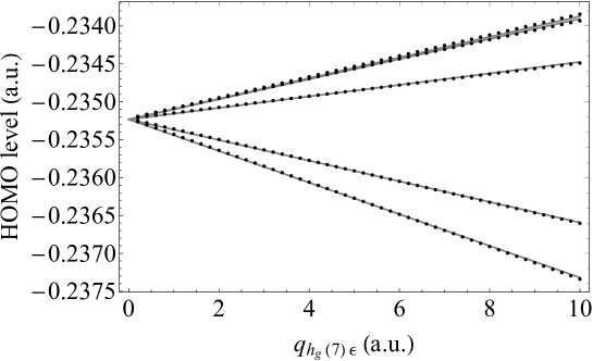
Figure 7: The JT splitting of the HOMO levels calculated by B3LYP with respect to $q_{h_{g}(7)\epsilon}$ deformation (in atomic unit). The black points and gray lines indicate the DFT values and model energy, respectively.

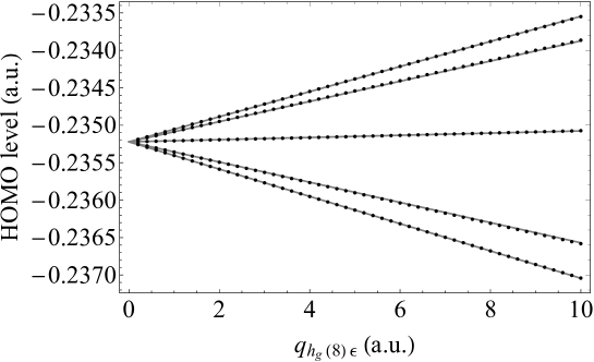
Figure 8: The JT splitting of the HOMO levels calculated by B3LYP with respect to $q_{h_{g}(8)\epsilon}$ deformation (in atomic unit). The black points and gray lines indicate the DFT values and model energy, respectively.

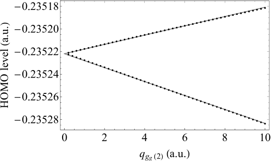
Figure 9: The JT splitting of the HOMO levels calculated by B3LYP with respect to $q_{g_{g}(2)\epsilon}$ deformation (in atomic unit). The black points and gray lines indicate the DFT values and model energy, respectively.

Figure 10: The JT splitting of the HOMO levels calculated by B3LYP with respect to $q_{g_{g}(3)\epsilon}$ deformation (in atomic unit). The black points and gray lines indicate the DFT values and model energy, respectively.

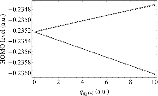
Figure 11: The JT splitting of the HOMO levels calculated by B3LYP with respect to $q_{g_{g}(4)\epsilon}$ deformation (in atomic unit). The black points and gray lines indicate the DFT values and model energy, respectively.

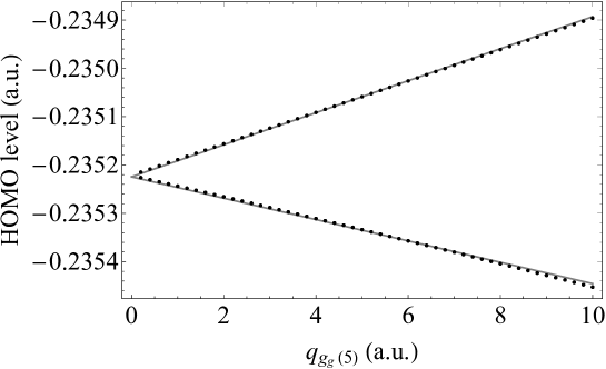
Figure 12: The JT splitting of the HOMO levels calculated by B3LYP with respect to $q_{g_{g}(5)\epsilon}$ deformation (in atomic unit). The black points and gray lines indicate the DFT values and model energy, respectively.

Figure 13: The JT splitting of the HOMO levels calculated by B3LYP with respect to $q_{g_{g}(6)\epsilon}$ deformation (in atomic unit). The black points and gray lines indicate the DFT values and model energy, respectively.

Considering CAM-B3LYP functional, Fig. 14, 15, 16, 17, 18, 19 and 20 depict the fitting of $q_{h_{g}(i)\epsilon},~{}i=2,3,4,5,6,7,8$, with Fig. 21, 22, 23, 24, and 25 for $q_{g_{g}(i)},~{}i=2,3,4,5,6$.

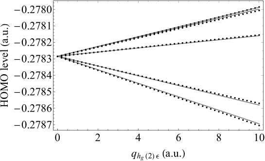
Figure 14: The JT splitting of the HOMO levels calculated by CAM-B3LYP with respect to $q_{h_{g}(2)\epsilon}$ deformation (in atomic unit). The black points and gray lines indicate the DFT values and model energy, respectively.

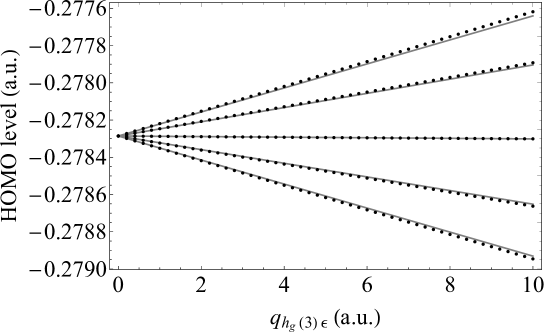
Figure 15: The JT splitting of the HOMO levels calculated by CAM-B3LYP with respect to $q_{h_{g}(3)\epsilon}$ deformation (in atomic unit). The black points and gray lines indicate the DFT values and model energy, respectively.

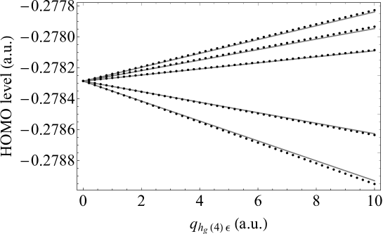
Figure 16: The JT splitting of the HOMO levels calculated by CAM-B3LYP with respect to $q_{h_{g}(4)\epsilon}$ deformation (in atomic unit). The black points and gray lines indicate the DFT values and model energy, respectively.

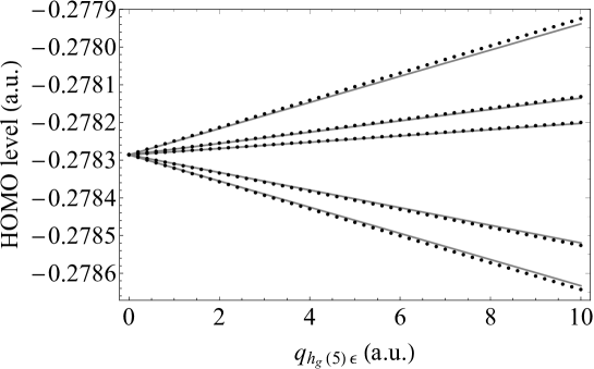
Figure 17: The JT splitting of the HOMO levels calculated by CAM-B3LYP with respect to $q_{h_{g}(5)\epsilon}$ deformation (in atomic unit). The black points and gray lines indicate the DFT values and model energy, respectively.

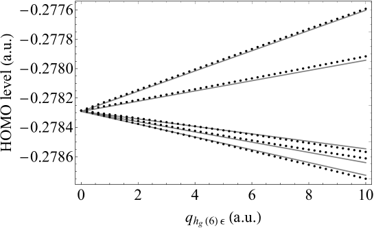
Figure 18: The JT splitting of the HOMO levels calculated by CAM-B3LYP with respect to $q_{h_{g}(6)\epsilon}$ deformation (in atomic unit). The black points and gray lines indicate the DFT values and model energy, respectively.

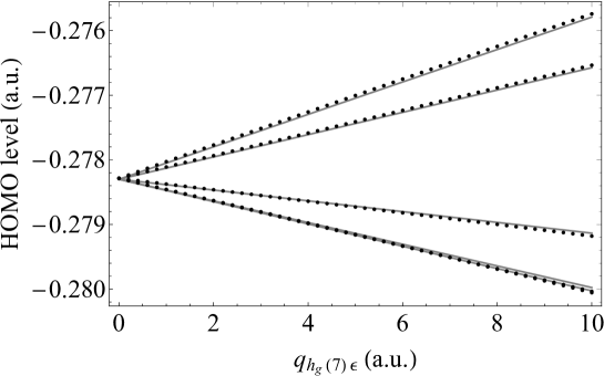
Figure 19: The JT splitting of the HOMO levels calculated by CAM-B3LYP with respect to $q_{h_{g}(7)\epsilon}$ deformation (in atomic unit). The black points and gray lines indicate the DFT values and model energy, respectively.

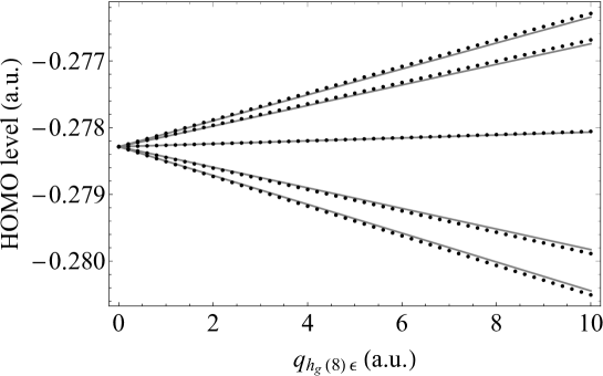
Figure 20: The JT splitting of the HOMO levels calculated by CAM-B3LYP with respect to $q_{h_{g}(8)\epsilon}$ deformation (in atomic unit). The black points and gray lines indicate the DFT values and model energy, respectively.

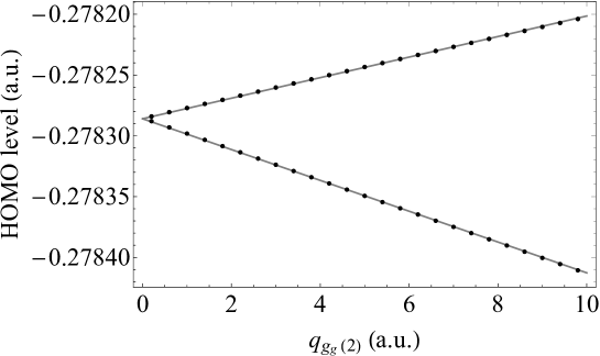
Figure 21: The JT splitting of the HOMO levels calculated by CAM-B3LYP with respect to $q_{g_{g}(2)\epsilon}$ deformation (in atomic unit). The black points and gray lines indicate the DFT values and model energy, respectively.

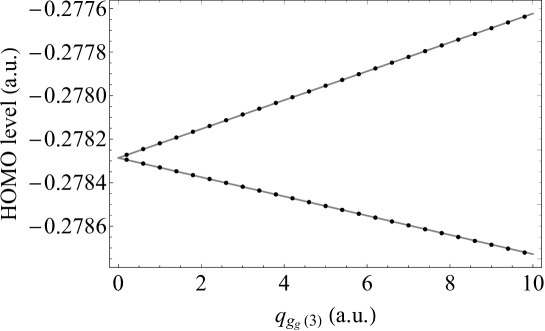
Figure 22: The JT splitting of the HOMO levels calculated by CAM-B3LYP with respect to $q_{g_{g}(3)\epsilon}$ deformation (in atomic unit). The black points and gray lines indicate the DFT values and model energy, respectively.

Figure 23: The JT splitting of the HOMO levels calculated by CAM-B3LYP with respect to $q_{g_{g}(4)\epsilon}$ deformation (in atomic unit). The black points and gray lines indicate the DFT values and model energy, respectively.

Figure 24: The JT splitting of the HOMO levels calculated by CAM-B3LYP with respect to $q_{g_{g}(5)\epsilon}$ deformation (in atomic unit). The black points and gray lines indicate the DFT values and model energy, respectively.

Figure 25: The JT splitting of the HOMO levels calculated by CAM-B3LYP with respect to $q_{g_{g}(6)\epsilon}$ deformation (in atomic unit). The black points and gray lines indicate the DFT values and model energy, respectively.

References

- Campbell et al. (2015) E. K. Campbell, M. Holz, D. Gerlich, and J. P. Maier, “Laboratory confirmation of C as the carrier of two diffuse interstellar bands,” Nature 523, 322 (2015).
- Campbell et al. (2016) E. K. Campbell, M. Holz, J. P. Maier, D. Gerlich, G. A. H. Walker, and D. Bohlender, “Gas Phase Absorption Spectroscopy of C and C in a Cryogenic Ion Trap: Comparison with Astronomical Measurements,” The Astrophysical Journal 822, 17 (2016).
- Spieler et al. (2017) S. Spieler, M. Kuhn, J. Postler, M. Simpson, R. Wester, P. Scheier, W. Ubachs, X. Bacalla, J. Bouwman, and H. Linnartz, “ and the Diffuse Interstellar Bands: An Independent Laboratory Check,” The Astrophysical Journal 846, 168 (2017).
- Yamada, Ross, and Ito (2017) K. M. Yamada, S. C. Ross, and F. Ito, “13C-substituted C: Predictions of the rotational spectra,” Molecular Astrophysics 6, 9 – 15 (2017).
- Strelnikov et al. (2018) D. V. Strelnikov, J. Jašík, D. Gerlich, M. Murata, Y. Murata, K. Komatsu, and J. Roithová, “Near- and Mid-IR Gas-Phase Absorption Spectra of H2@C-He,” The Journal of Physical Chemistry A 122, 8162–8166 (2018).
- Kaiser et al. (2018) A. Kaiser, J. Postler, M. Ončák, M. Kuhn, M. Renzler, S. Spieler, M. Simpson, M. Gatchell, M. K. Beyer, R. Wester, F. A. Gianturco, P. Scheier, F. Calvo, and E. Yurtsever, “Isomeric Broadening of C Electronic Excitation in Helium Droplets: Experiments Meet Theory,” The Journal of Physical Chemistry Letters 9, 1237–1242 (2018).
- Lykhin, Ahmadvand, and Varganov (2019) A. O. Lykhin, S. Ahmadvand, and S. A. Varganov, “Electronic Transitions Responsible for C Diffuse Interstellar Bands,” The Journal of Physical Chemistry Letters 10, 115–120 (2019).
- Cordiner et al. (2019) M. A. Cordiner, H. Linnartz, N. L. J. Cox, J. Cami, F. Najarro, C. R. Proffitt, R. Lallement, P. Ehrenfreund, B. H. Foing, T. R. Gull, P. J. Sarre, and S. B. Charnley, “Confirming interstellar c using the hubble space telescope,” The Astrophysical Journal 875, L28 (2019).
- Chancey and O’Brien (1997) C. C. Chancey and M. C. M. O’Brien, The Jahn–Teller Effect in C60 and Other Icosahedral Complexes (Princeton University Press, Princeton, 1997).
- Bersuker (2006) I. B. Bersuker, The Jahn–Teller Effect (Cambridge University Press, Cambridge, 2006).
- Brühwiler et al. (1997) P. A. Brühwiler, A. J. Maxwell, P. Baltzer, S. Andersson, D. Arvanitis, L. Karlsson, and N. Mårtensson, “Vibronic coupling in the photoemission bands of condensed C60,” Chemical Physics Letters 279, 85 – 91 (1997).
- Canton et al. (2002) S. E. Canton, A. J. Yencha, E. Kukk, J. D. Bozek, M. C. A. Lopes, G. Snell, and N. Berrah, “Experimental Evidence of a Dynamic Jahn-Teller Effect in ,” Phys. Rev. Lett. 89, 045502 (2002).
- Kern et al. (2013) B. Kern, D. Strelnikov, P. Weis, A. Böttcher, and M. M. Kappes, “IR Absorptions of C and C in Neon Matrixes,” J. Phys. Chem. A 117, 8251 (2013).
- Ceulemans and Fowler (1990) A. Ceulemans and P. W. Fowler, “The Jahn-Teller instability of fivefold degenerate states in icosahedral molecules,” The Journal of Chemical Physics 93, 1221–1234 (1990).
- Moate et al. (1996) C. P. Moate, M. C. M. O’Brien, J. L. Dunn, C. A. Bates, Y. M. Liu, and V. Z. Polinger, “: A Jahn-Teller Coupling That Really Does Reduce the Degeneracy of the Ground State,” Phys. Rev. Lett. 77, 4362–4365 (1996).
- De Los Rios, Manini, and Tosatti (1996) P. De Los Rios, N. Manini, and E. Tosatti, “Dynamical Jahn-Teller effect and Berry phase in positively charged fullerenes: Basic considerations,” Phys. Rev. B 54, 7157–7167 (1996).
- Manini, Gattari, and Tosatti (2003) N. Manini, P. Gattari, and E. Tosatti, “Jahn-Teller Spectral Fingerprint in Molecular Photoemission: ,” Phys. Rev. Lett. 91, 196402 (2003).
- Lijnen and Ceulemans (2005) E. Lijnen and A. Ceulemans, “Berry phase and entanglement in the icosahedral Jahn-Teller system with trigonal minima,” Phys. Rev. B 71, 014305 (2005).
- Hands et al. (2006a) I. D. Hands, L. M. Sindi, J. L. Dunn, and C. A. Bates, “Theoretical treatment of pseudorotation in the Jahn-Teller ion,” Phys. Rev. B 74, 115410 (2006a).
- Hands et al. (2006b) I. D. Hands, J. L. Dunn, W. A. Diery, and C. A. Bates, “Vibronic coupling in the icosahedral Jahn-Teller cation: Repercussions of the nonsimple reducibility of the product,” Phys. Rev. B 73, 115435 (2006b).
- Hands et al. (2007) I. D. Hands, W. A. Diery, C. A. Bates, and J. L. Dunn, “Jahn-teller effects in the cation undergoing distortion,” Phys. Rev. B 76, 085426 (2007).
- Ceulemans et al. (2012) A. Ceulemans, E. Lijnen, P. W. Fowler, R. B. Mallion, and T. Pisanski, “S5 graphs as model systems for icosahedral jahn-teller problems,” Theoretical Chemistry Accounts 131 (2012), 10.1007/s00214-012-1246-3.
- Manini et al. (2001) N. Manini, A. D. Corso, M. Fabrizio, and E. Tosatti, “Electron-vibration coupling constants in positively charged fullerene,” Philosophical Magazine B 81, 793–812 (2001).
- Saito (2002) M. Saito, “Electron-phonon coupling of electron- or hole-injected ,” Phys. Rev. B 65, 220508 (2002).
- Ramanantoanina et al. (2013) H. Ramanantoanina, M. Zlatar, P. García-Fernández, C. Daul, and M. Gruden-Pavlović, “General treatment of the multimode jahn-teller effect: study of fullerene cations,” Phys. Chem. Chem. Phys. 15, 1252–1259 (2013).
- Iwahara et al. (2010) N. Iwahara, T. Sato, K. Tanaka, and L. F. Chibotaru, “Vibronic coupling in anion revisited: Derivations from photoelectron spectra and DFT calculations,” Phys. Rev. B 82, 245409 (2010).
- Faber et al. (2011) C. Faber, J. L. Janssen, M. Côté, E. Runge, and X. Blase, “Electron-phonon coupling in the C60 fullerene within the many-body approach,” Phys. Rev. B 84, 155104 (2011).
- Huang and Liu (2020) Z. Huang and D. Liu, “Dynamical jahn-teller effect in the first excited c,” International Journal of Quantum Chemistry 120, e26148 (2020).
- Kroto et al. (1985) H. W. Kroto, J. R. Heath, S. C. O’Brien, R. F. Curl, and R. E. Smalley, “C60: Buckminsterfullerene,” Nature 318, 162–163 (1985).
- Jahn and Teller (1937) H. A. Jahn and E. Teller, “Stability of Polyatomic Molecules in Degenerate Electronic States. I. Orbital Degeneracy,” Proc. R. Soc. Lond. A 161, 220 (1937).
- Inui, Tanabe, and Onodera (1990) T. Inui, Y. Tanabe, and Y. Onodera, Group Theory and Its Applications in Physics (Springer-Verlag, Berlin and Heidelberg, 1990).
- Liu et al. (2018) D. Liu, Y. Niwa, N. Iwahara, T. Sato, and L. F. Chibotaru, “Quadratic Jahn-Teller effect of fullerene anions,” Phys. Rev. B 98, 035402 (2018).
- Laflamme Janssen et al. (2010) J. Laflamme Janssen, M. Côté, S. G. Louie, and M. L. Cohen, “Electron-phonon coupling in using hybrid functionals,” Phys. Rev. B 81, 073106 (2010).
- Fetter and Walecka (2003) A. L. Fetter and D. Walecka, Quantum Theory of Many-Particle Systems (Dover Publishing, Inc., New York, 2003).
- Frisch et al. (2016) M. J. Frisch, G. W. Trucks, H. B. Schlegel, G. E. Scuseria, M. A. Robb, J. R. Cheeseman, G. Scalmani, V. Barone, G. A. Petersson, H. Nakatsuji, X. Li, M. Caricato, A. V. Marenich, J. Bloino, B. G. Janesko, R. Gomperts, B. Mennucci, H. P. Hratchian, J. V. Ortiz, A. F. Izmaylov, J. L. Sonnenberg, D. Williams-Young, F. Ding, F. Lipparini, F. Egidi, J. Goings, B. Peng, A. Petrone, T. Henderson, D. Ranasinghe, V. G. Zakrzewski, J. Gao, N. Rega, G. Zheng, W. Liang, M. Hada, M. Ehara, K. Toyota, R. Fukuda, J. Hasegawa, M. Ishida, T. Nakajima, Y. Honda, O. Kitao, H. Nakai, T. Vreven, K. Throssell, J. A. Montgomery, Jr., J. E. Peralta, F. Ogliaro, M. J. Bearpark, J. J. Heyd, E. N. Brothers, K. N. Kudin, V. N. Staroverov, T. A. Keith, R. Kobayashi, J. Normand, K. Raghavachari, A. P. Rendell, J. C. Burant, S. S. Iyengar, J. Tomasi, M. Cossi, J. M. Millam, M. Klene, C. Adamo, R. Cammi, J. W. Ochterski, R. L. Martin, K. Morokuma, O. Farkas, J. B. Foresman, and D. J. Fox, “Gaussian˜16 Revision C.01,” (2016), gaussian Inc. Wallingford CT.
- Liehr (1963) A. D. Liehr, “Topological aspects of the conformational stability problem. Part I. Degenerate electronic states,” J. Phys. Chem. 67, 389 (1963).
- Khlopin, Polinger, and Bersuker (1978) V. P. Khlopin, V. Z. Polinger, and I. B. Bersuker, “The jahn-teller effect in icosahedral molecules and complexes,” Theoretica chimica acta 48, 87–101 (1978).
- Bersuker and Polinger (1989) I. B. Bersuker and V. Z. Polinger, Vibronic Interactions in Molecules and Crystals (Springer–Verlag, Berlin, 1989).
- Bruyndonckx et al. (1997) R. Bruyndonckx, C. Daul, P. T. Manoharan, and E. Deiss, “A nonempirical approach to ground-state jahn-teller distortion: Case study of vcl4,” Inorganic Chemistry 36, 4251–4256 (1997).
- Zlatar, Schläpfer, and Daul (2009) M. Zlatar, C.-W. Schläpfer, and C. Daul, “A new method to describe the multimode jahn-teller effect using density functional theory,” in The Jahn-Teller Effect (Springer, 2009) pp. 131–165.
- Zlatar et al. (2010) M. Zlatar, M. Gruden-Pavlović, C.-W. Schläpfer, and C. Daul, “Intrinsic distortion path in the analysis of the jahn-teller effect,” Journal of Molecular Structure: THEOCHEM 954, 86–93 (2010).
- Zlatar and Gruden (2019) M. Zlatar and M. Gruden, “Calculation of the jahn-teller parameters with dft,” 2019 , 1 (2019).
- Muya et al. (2013) J. T. Muya, H. Ramanantoanina, C. Daul, M. T. Nguyen, G. Gopakumar, and A. Ceulemans, “Jahn-Teller instability in cationic boron and carbon buckyballs B and C: a comparative study,” Phys. Chem. Chem. Phys. 15, 2829–2835 (2013).
- Sato, Tokunaga, and Tanaka (2006) T. Sato, K. Tokunaga, and K. Tanaka, “Vibronic coupling in cyclopentadienyl radical: A method for calculation of vibronic coupling constant and vibronic coupling density analysis,” J. Chem. Phys. 124, 024314 (2006).
- Sato, Tokunaga, and Tanaka (2008) T. Sato, K. Tokunaga, and K. Tanaka, “Vibronic Coupling in Naphthalene Anion: Vibronic Coupling Density Analysis for Totally Symmetric Vibrational Modes,” J. Phys. Chem. A 112, 758 (2008).
- Sato, Iwahara, and Tanaka (2012) T. Sato, N. Iwahara, and K. Tanaka, “Critical reinvestigation of vibronic couplings in picene from view of vibronic coupling density analysis,” Phys. Rev. B 85, 161102 (2012).
- Matsuda et al. (2018) Y. Matsuda, N. Iwahara, K. Tanigaki, and L. F. Chibotaru, “Manifestation of vibronic dynamics in infrared spectra of mott insulating fullerides,” Phys. Rev. B 98, 165410 (2018).
- Ponzellini (2014) P. Ponzellini, Computation of the paramagnetic g-factor for the fullerene monocation and monoanion, Master’s thesis, Milan University (2014).
- Gunnarsson et al. (1995) O. Gunnarsson, H. Handschuh, P. S. Bechthold, B. Kessler, G. Ganteför, and W. Eberhardt, “Photoemission Spectra of C: Electron-Phonon Coupling, Jahn-Teller Effect, and Superconductivity in the Fullerides,” Phys. Rev. Lett. 74, 1875 (1995).
- Wang, Woo, and Wang (2005) X.-B. Wang, H.-K. Woo, and L.-S. Wang, “Vibrational cooling in a cold ion trap: Vibrationally resolved photoelectron spectroscopy of cold C anions,” J. Chem. Phys. 123, 051106 (2005).
- Huang et al. (2014) D. L. Huang, P. D. Dau, H. T. Liu, and L. S. Wang, “High-resolution photoelectron imaging of cold C anions and accurate determination of the electron affinity of C60,” J Chem Phys 140, 224315 (2014).
- Iwahara and Chibotaru (2013) N. Iwahara and L. F. Chibotaru, “Dynamical Jahn-Teller Effect and Antiferromagnetism in ,” Phys. Rev. Lett. 111, 056401 (2013).
- Liu, Iwahara, and Chibotaru (2018) D. Liu, N. Iwahara, and L. F. Chibotaru, “Dynamical jahn-teller effect of fullerene anions,” Phys. Rev. B 97, 115412 (2018).
- Shizu, Sato, and Tanaka (2010) K. Shizu, T. Sato, and K. Tanaka, “Inelastic electron tunneling spectra and vibronic coupling density analysis of 2,5-dimercapto-1,3,4-thiadiazole and tetrathiafulvalene dithiol,” Nanoscale 2, 2186–2194 (2010).
- Frederiksen et al. (2008) T. Frederiksen, K. J. Franke, A. Arnau, G. Schulze, J. I. Pascual, and N. Lorente, “Dynamic Jahn-Teller effect in electronic transport through single molecules,” Phys. Rev. B 78, 233401 (2008).
- Große et al. (2017) C. Große, P. Merino, A. Rosławska, O. Gunnarsson, K. Kuhnke, and K. Kern, “Submolecular Electroluminescence Mapping of Organic Semiconductors,” ACS Nano 11, 1230–1237 (2017).
- Latzke et al. (2019) D. W. Latzke, C. Ojeda-Aristizabal, J. D. Denlinger, R. Reno, A. Zettl, and A. Lanzara, “Orbital character effects in the photon energy and polarization dependence of pure c60 photoemission,” ACS Nano 13, 12710–12718 (2019).
- Qiu, Chibotaru, and Ceulemans (2001) Q. C. Qiu, L. F. Chibotaru, and A. Ceulemans, “Product jahn-teller systems: The icosahedral exciton,” Phys. Rev. B 65, 035104 (2001).
- Akimoto and Kan’no (2002) I. Akimoto and K.-i. Kan’no, “Photoluminescence and Near-Edge Optical Absorption in the Low-Temperature Phase of Pristine C60 Single Crystals,” Journal of the Physical Society of Japan 71, 630–643 (2002).
- Stepanov et al. (2002) A. G. Stepanov, M. T. Portella-Oberli, A. Sassara, and M. Chergui, “Ultrafast intramolecular relaxation of C60,” Chemical Physics Letters 358, 516 – 522 (2002).
Supplement Material: First principles study of the vibronic coupling in positively charged C
Zhishuo Huang1,a) and Dan Liu2,1,b)
1Theory of Nanomaterials Group, KU Leuven, Celestijnenlaan 200F, B-3001 Leuven, Belgium
2Institute of Flexible Electronics (IFE), Northwestern Polytechnical University, 127 West Youyi Road, Xi’an, 710072, Shaanxi, China
a)Electronic address: zhishuohuang@gmail.com
b)Electronic address: iamdliu@nwpu.edu.cn