QKD in Isabelle – Bayesian Calculation

Abstract

In this paper, we present a first step towards a formalisation of the Quantum Key Distribution algorithm in Isabelle. We focus on the formalisation of the main probabilistic argument why Bob cannot be certain about the key bit sent by Alice before he doesn’t have the chance to compare the chosen polarization scheme. This means that any adversary Eve is in the same position as Bob and cannot be certain about the transmitted keybits. We introduce the necessary basic probability theory, present a graphical depiction of the protocol steps and their probabilities, and finally how this is translated into a formal proof of the security argument.

1 Introduction

In this paper, we present a simple finite foundation for a formalisation of parts of the Quantum Key Distribution (QKD) algorithm in Isabelle. We focus on the formalisation of the probabilistic theory needed to formalise and then calculate the probability with which Bob receives the key bit sent by Alice. This basic probability argument is important as it can also be applied to the attacker Eve that has the same chance to learn the transmitted keybits. Bob, however, in a second step compares the used polarisation schemes with Alice. Thereby he and Alice are able to retain only key bits that have been correctly transmitted.

To give a brief idea of the protocol that can be used to transmit a sequence of random bits (that can then be used as a shared One-Time-Pad key giving 100% security):

• Alice randomly selects a bit 0 or 1

• Alice randomly chooses diagonal (X) or rectilinear (+) polarisation schemes to encode the bit as a photon before sending the bit

• Bob also randomly chooses schemes (X/+) before measuring the received photon. According to quantum properties, if Alice and Bob chose the same polarisation schemes the transmission is 100% correct, if they use different ones the changes are 50/50.

A representative list of possible combinations is given in Figure 1.

Alice sends

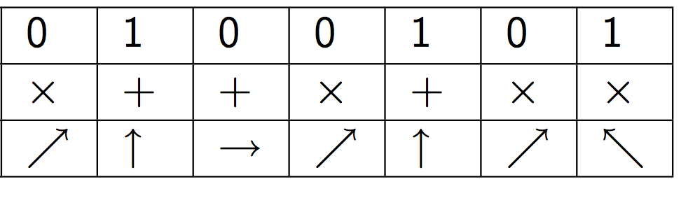
Bob measures

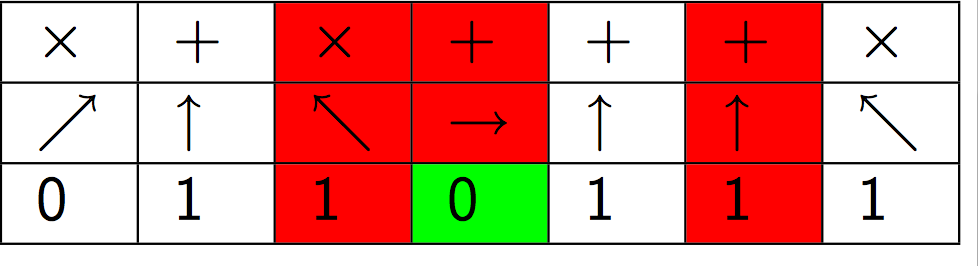
they can use

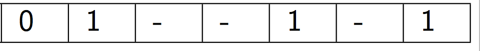
Figure 1: QKD example (images from [4])

In this paper, we (1) introduce the necessary probability theory to show (2) the basic probabilities of the correctness of the key transmission in the protocol which is a step towards the security analysis and (3) we develop and illustrate the probability reasoning on finite sets of outcomes in Isabelle. Note, that we consider only one bit since the principle is the same in any number of repetitions necessary to transmit a $n$-bit key. Also we only consider for a start the first phase of the protocol.

We introduce the necessary basic probability theory, present a graphical depiction of the protocol steps and their probabilities, and finally show how this is translated into a formal proof of the security argument. The theory and all presented proofs are formalised in Isabelle (see Appendix).

1.1 Basic Probability

The very brief introduction to basic probability theory is taken from Koller and Friedmann [3] but vastly abbreviated. The reader is referred to this excellent textbook for details.

Before defining events $({\mathcal{S}})$ we first assume a set $\Omega$ of possible outcomes. Based on that we define a set of measurable events ${\mathcal{S}}\subseteq{\mathcal{P}}\Omega$ where ${\mathcal{P}}$ is the power set. Any event $A\in{\mathcal{S}}$ may have probabilities assigned to it. Probability theory, more precisely, measure theory (see [1]), requires that the the following conditions hold for the probability space ${\mathcal{S}}$:

• ${\mathcal{S}}$ contains the empty event $\varnothing$ and the trivial event $\Omega$;

• ${\mathcal{S}}$ must be closed under union: $A,B\in evs\mbox{{$\Rightarrow$}}A\cup B\in evs$;

• ${\mathcal{S}}$ must be closed under complement: $A\in evs\mbox{{$\Rightarrow$}}\Omega\setminus A\in evs$.

The closure for the other Boolean operators intersection and set difference is implied by the above conditions.

Definition 1.1 (Probability Distribution).

A probability distribution $P$ over $(\Omega,{\mathcal{S}})$ is a function from events in ${\mathcal{S}}$ to real numbers satisfying the following conditions.

1. $\forall A\in{\mathcal{S}}.\ P(A)\geq 0$.

2. $P(\Omega)=1$.

3. If $A,B\in{\mathcal{S}}$ and $A\cap B=\varnothing$ then $P(A\cup B)=P(A)+P(B)$.

In Joe Hurd’s dissertation [1] these conditions are referred to as

• Positivity,

• Probability space ((2.27), page 33 [1]), and

• Additivity

in the general context of Measure spaces. The property of Monotonocity and Countable Additivity [1] are not present in the introduction of Koller and Friedman but at least Countable Additivity can be considered as implicit since we are looking at finite spaces only.

The above definition can be directly translated into an Isabelle specification. We transform the textbook definition into a definition and a type definition: we define first event spaces over finite types of outcomes and then we give a type definition for probability distribution.

The possible outcomes can be provided as a type represented here by a type variable $\Omega$. This type is assumed to be finite implicitly by coercing the type variable $\Omega$ into the type class finite using the type judgment with :: in the following definition of probability space. definition prob_space :: (($\Omega$ :: finite) set) set) $\Rightarrow$ bool where prob_space ${\mathcal{S}}$ = {} $\in$ ${\mathcal{S}}$ $\land$ (UNIV :: $\Omega$ set) $\in$ ${\mathcal{S}}$ $\land$ $\forall$ A, B $\in$ ${\mathcal{S}}$. A $\cup$ B $\in$ ${\mathcal{S}}$ $\land$ $\forall$ A $\in$ ${\mathcal{S}}$. (UNIV :: $\Omega$ set) - A $\in$ ${\mathcal{S}}$ In the above type definition, the $\Omega$ is an Isabelle type variable. The polymorphic constructor UNIV is a standard constructor in Isabelle and represents the set of all elements of a type, here all outcomes in $\Omega$. We can now show that the powerset over a finite type is a probability space. theorem Pow_prob_space: "$\forall$ (A :: ($\Omega$::finite) set). prob_space (Pow A)" A probability distribution is a function over a probability space. We use a type definition for it. typedef ($\Omega$ :: finite) prob_dist = {p :: ($\Omega$ set $\Rightarrow$ real). $\forall$ (A :: $\Omega$ set). p A $\geq$ 0 $\land$ p(UNIV :: $\Omega$ set) = 1 $\land$ $\forall$ (A :: $\Omega$ set) B . A $\cap$ B = $\varnothing$ $\longrightarrow$ p(A $\cup$ B) = p(A) + p(B) } In the above type definition for probability distribution, we can see that the three criteria from Definition 1.1 are almost one to one translated into Isabelle. Type definitions are applied by imposing them on new constants or variables which automatically leads to the invocation of the defining properties on these elements: either by assuming them for constants defined over the new types or by creating new proof obligations when existing terms are judged to be of these types. We apply this when we define a probability distribution over the power set of a finite type of outcomes for QKD in Section 4.

Hurd already writes “Measure theory defines what probability spaces are but does little to help us find concrete distributions”[1]. He then uses Caratheodory’s extension theorem to help out. For the simple case of finite sets of outcomes that we consider here, we introduce a canonical construction that uses the powerset of outcomes as the event space and accordingly constructs the probability distribution by summing up the probabilities for the individual outcomes of any subset of $\Omega$, i.e. an event $\in{\mathcal{S}}$, which is possible since they are finite sets and the outcomes are all distinct. For the definition of a generic operator for this canonical construction, we use the fold operator available in Isabelle for defining simple recursive functions over finite sets. Intuitively, fold operates like this:

$$\text{{fold}}\ f\ z\ \{x_{1},\dots,x_{n}\}=f(x_{1}\dots(f\ x_{n}\ z))\,.$$

We define the canonical construction for probability distributions as a function pmap lifting a probability assignment ops for single outcomes $\mbox{{$\in$}}\Omega$ to any set S. pmap (ops :: $\Omega$ $\Rightarrow$ real) S = fold ($\lambda$ x y. ops x + y) 0 S Now, we can show that for any finite type $\Omega::\texttt{finite}$ with a probability assignment ops the canonical construction yields a probability distribution over the power set by showing that it is contained in the defining set of the type prob_dist given by the domain of the internal type injection Rep_prob_dist. theorem pmap_ops: pmap ops $\in$ dom Rep_prob_dist $\land$ $\forall$ x :: $\Omega$. pmap ops {x} = ops x

Conditional probability, for example, $P(A|B)$ signifies the probability for an event $A$ given an event $B$. It can be defined simply as follows.

Definition 1.2 (Conditional Probability).

For an event space ${\mathcal{S}}$ and two events $A,B\in{\mathcal{S}}$ the conditional probability of $A$ given $B$ is defined for a probability distribution $P$ as

$$P(A|B)\equiv P(A\cap B)/P(B)\,.$$

The corresponding Isabelle definition uses some syntactic sugaring to hide the fact that the mathematical definition above is somewhat sloppy in its types. definition cond_prob :: ($\Omega$ :: finite)prob_dist $\Rightarrow$ $\Omega$ set $\Rightarrow$ $\Omega$ set $\Rightarrow$ real "_(_|_)" where P(A|B) $\equiv$ (Rep_prob_dist P (A $\cap$ B)) / (Rep_prob_dist P B) The above Isabelle definition uses the mixfix syntax after the type in quotation marks to allow writing the same probability distribution as a function with two arguments by a syntactic translation into the corresponding definition with intersections of the event sets.

2 Protocol Tree with Probabilities

Figure 2: Decision tree for QKD: probabilities for each step at edges and outcome probabilities as leaves.

The tree depicted in Figure 2 shows the probabilities along the paths from root to leaves according to the steps of the protocol.

How does a concrete application, like QKD, relate to the probabilities and distributions encountered previously? The outcomes we consider are Boolean vectors of length four representing each one a possible path of the protocol. The following type of QKD_om will instantiate the polymorphic type $\Omega$ in the previous definitions. type_synonym QKD_om = bool * bool * bool * bool To make the outcomes more readable we introduce the following abbreviations as local definition of the locale QKD [2]. Their intended meaning is AsOne: “A sends 1”, AchX/BchX: “A/B chooses diagonal scheme” and BmOne” “B measures 1”. locale QKD = defines AsOne out = fst(out) AchX out = fst(snd out) BchX out = fst(snd(snd out)) BmOne out = snd(snd(snd out)) The basic distribution on these 16 outcomes derived from Figure 2 is given in the table in Figure 3.

AsOne	AchX	BchX	BmOne	P
False	False	False	False	1/8
False	False	False	True	0
False	False	True	False	1/16
False	False	True	True	1/16
False	True	False	False	1/16
False	True	False	True	1/16
False	True	True	False	1/8
False	True	True	True	0
True	False	False	False	0
True	False	False	True	1/8
True	False	True	False	1/16
True	False	True	True	1/16
True	True	False	False	1/16
True	True	False	True	1/16
True	True	True	False	0
True	True	True	True	1/8

Figure 3: Probability assignment for QKD outcomes

This basic probability distribution can be input as the element ops in the above function pmap producing automatically the canonical probability distribution for the QKD protocol. To define the basic function ops, we use a locale definition [2]. We omit the details of the cases as they are clear from the table in Figure 3 (see Appendix). defines (qkd_ops :: QKD_om $\Rightarrow$ real) = $\lambda$ x. case x of (False, False, False, False) $\Rightarrow$ 1/8 | ... We can then define a probability distribution being able to show that it is in fact one by Theorem pmap_ops. defines (qkd_prob_dist :: prob_dist) = pmap qkd_ops Based on this probability distribution we can calculate interesting probabilities telling us something about the security of the protocol.

In order to do that we first consider another useful probability law: the law of total probability.

3 Law of Total Probability

For the Security Argument, we need the law of total probability.

Theorem 1 (Law of total probability).

Let $A_{j},j\leq n$ for some $n\in\mathbb{N}$ be a set of events partitioning the event space ${\mathcal{S}}$, that is, $\forall\ i,j\leq n.\ i\neq j\mbox{{$\Rightarrow$}}A_{i}\cap A_{j}=\varnothing$ and $\bigcup_{j}A_{j}=\Omega$. Let further $B\in evs$. We then have that

$$P(B)=\sum_{j}P(B|A_{j})P(A_{j})\,.$$

Proof.

Since we have a partition, that is, $A_{i}\cap A_{j}=\varnothing$ for all $i,j\leq n$ with $i\neq j$, we have also

$$\begin{array}[]{ccccccccr}(B\cap A_{i})\cap(B\cap A_{j})&=&B\cap(A_{i}\cap A_{j})&=&B\cap\varnothing&=&\varnothing&\qquad\qquad(1)\end{array}$$

Therefore

$$\begin{array}[]{clll}P(B)&=&P(B\cap\Omega)&{(A_{j}\ \text{is partition of }\Omega)}\\ &=&P(B\cap(A_{1}\cup\dots\cup A_{n}))&(\text{set algebra})\\ &=&P((B\cap A_{1})\cup\dots\cup(B\cap A_{n}))&((1)\text{ and Definition \ref{def:dist} (3)})\\ &=&P(B\cap A_{1})+\dots+P(B\cap A_{n})&(\text{summation})\\ &=&\sum_{j}P(B\cap A_{j})&(\text{Definition of conditional probability})\\ &=&\sum_{j}P(B|A_{j})*P(A_{j})&\\ \end{array}$$

∎

4 Security Argument

The first argument computes the probability that B measures 1 applying the law of total probability. The partition ${\mathcal{A}}$ of $\Omega$ used in the derivation is given as the following family of disjoint sets with $\bigcup{\mathcal{A}}=\Omega$.

$$\begin{array}[]{lll}{\mathcal{A}}&=&\{\{s::\texttt{QKD\_om}.\ \texttt{BchX}\ s\wedge\texttt{AchX}\ s\wedge\texttt{AsOne}\ s\},\\ &&\ \{s::\texttt{QKD\_om}.\ \neg(\texttt{BchX}\ s)\wedge\texttt{AchX}\ s\wedge\texttt{AsOne}\ s\},\\ &&\ \{s::\texttt{QKD\_om}.\ \texttt{BchX}\ s\wedge\neg(\texttt{AchX}\ s)\wedge\texttt{AsOne}\ s\},\\ &&\ \{s::\texttt{QKD\_om}.\ \neg(\texttt{BchX})\ s\wedge\neg(\texttt{AchX}\ s)\wedge\texttt{AsOne}\ s\},\\ &&\ \{s::\texttt{QKD\_om}.\ \texttt{BchX}\ s\wedge\texttt{AchX}\ s\wedge\neg(\texttt{AsOne})\ s\},\\ &&\ \{s::\texttt{QKD\_om}.\ \neg(\texttt{BchX}\ s)\wedge\texttt{AchX}\ s\wedge\neg(\texttt{AsOne})\ s\},\\ &&\ \{s::\texttt{QKD\_om}.\ \texttt{BchX}\ s\wedge\neg(\texttt{AchX}\ s)\wedge\neg(\texttt{AsOne})\ s\},\\ &&\ \{s::\texttt{QKD\_om}.\ \neg(\texttt{BchX})\ s\wedge\neg(\texttt{AchX}\ s)\wedge\neg(\texttt{AsOne})\ s\}\\ &&\}\end{array}$$

For each $A_{j}\in{\mathcal{A}}$, we have $P(A_{j})=1/8$: since $P$ is a probability distribution, we can use the third defining property to sum up the disjoint probabilities for each outcome. The outcome probabilities in Figure 3 give for example (similar for the other $A_{j}$):

$$\begin{array}[]{ll}P(\{s::\texttt{QKD\_om}.\ \texttt{BchX}\ s\wedge\texttt{AchX}\ s\wedge\texttt{AsOne}\ s\})&=\\ P(\texttt{True},\texttt{True},\texttt{True},\texttt{True})+P(\texttt{True},\texttt{True},\texttt{True},\texttt{False})&=\\ 1/8+0=1/8&\\ \end{array}$$

With this we can compute that $P(\texttt{BmOne})=1/2$.

$$\begin{array}[]{clll}P(\texttt{BmOne})&=&\sum_{A_{j}\in\mathcal{A}}P(\texttt{BmOne}|A_{j})*P(A_{j})&(\text{Law of total probability})\\ &=&1/8*\sum_{A_{j}\in\mathcal{A}}P(\texttt{BmOne}|A_{j})&(P(A_{j})=1/8)\\ &=&1/8*\sum_{A_{j}\in\mathcal{A}}P(\texttt{BmOne}\cap A_{j})/P(A_{j})&(\texttt{Definition }\ref{def:condprob})\\ &=&\sum_{A_{j}\in\mathcal{A}}P(\texttt{BmOne}\cap A_{j})&(P(A_{j})=1/8)\\ &=&1/2&(\text{sum even columns in Table }\ref{fig:table})\end{array}$$

This probability cannot be interpreted as a security statement directly. It rather says that on the whole Bob receives 1s with 50% probability but not how this relates to what A has actually sent. However the above probability $P(\texttt{BmOne})$ is useful to calculate the conditional probability $P(\texttt{AsOne}|\texttt{BmOne})$: how likely is it that A has actually sent a 1 given that B received a 1?

$$\begin{array}[]{clll}P(\texttt{AsOne}|\texttt{BmOne})&=&P(\texttt{AsOne}\cap\texttt{BmOne})/P(\texttt{BmOne})&(\text{Conditional Probability})\\ &=&2*(P(\{x::\mbox{$\Omega$}.\ \texttt{AsOne }x\wedge\texttt{BmOne }x\}))&(\text{above calculation})\\ &=&2*(P(\{\{\texttt{T,F,F,T}\},\{\texttt{T,F,T,T}\},&\\ &&\qquad\quad\{\texttt{T,T,F,T}\},\{\texttt{T,T,T,T}\}\}))&(\text{Definition \ref{def:dist}})\\ &=&2*(P(\{\{\texttt{T,F,F,T}\})+P(\{\texttt{T,F,T,T}\})+&\\ &&\qquad\quad P(\{\texttt{T,T,F,T}\})+P(\{\texttt{T,T,T,T}\}))&(\text{Table \ref{fig:table}})\\ &=&2*(1/8+1/16+1/16+1/8)&(\texttt{arithmetic})\\ &=&3/4\\ \end{array}$$

This shows that there is 25% chance of error for Bob and Eve to receive the wrong bit.

5 Conclusion

We have provided a simple probability model for Isabelle based on finite outcome types formalising basic Bayesian probability notions, proving general theorems and illustrating their use on the application of QKD. It is interesting to observe that the mathematical model for the quantum computations realising the protocol behaviour seems not present: it is embedded in the a priori probabilities of the basic outcomes in Table 3. This is a nice (and important) observation since the present formalisation shows that the actual quantum model and the probability model can be treated in a modular manner.

The security argument presented so far is actually rather poor: with 75% probability the attacker Eve and Bob can assume that they have got the right bit. This is not enough protection for security. The security relies on one further observation and an additional protocol step. The observation is that if Eve resends the bit she has received, Bob – when measuring afterwards – will have erroneous measurements even in the case that should give the right results with 100% probability. This error can be revealed in the additional protocol step in which Alice and Bob compare (first the used polarisation schemes and then based on that) some portion of the bits they transmitted coincidentally with equal schemes.

To model and analyse the probabilities for the intercept and resend attack, the finite probability model presented her is sufficient: we just need to extend the outcome type and add the corresponding a priori probabilities to an extended Table 3. This will allow to calculate the final error probability when Eve intercepts and resends. However, for the final security argument that proves the “unconditional security” of QKD (assuming the clear line isn’t intercepted) the probability model over finite outcome types needs to be extended to outcomes that are infinite sequences. This will then necessitate a model similar to the one in Hurd’s thesis [1].

Appendix A Isabelle Code

under construction

References

- [1] J. Hurd. Formal verification of probabilistic algorithms. Technical Report 566, University of Cambridge, 2001.
- [2] F. Kammüller. Modular reasoning in isabelle. In D. MacAllester, editor, 17th International Conference on Automated Deduction, CADE-17, volume 1831 of LNAI. Springer, 2000.
- [3] D. Koller and N. Friedman. Probabilistic Graphical Models – Principles and Techniques. The MIT Press, 2009.
- [4] S. Singh. The Code Book. Fourth Estate, 4 edition, 1999.