Robust Simultaneously Stabilizing Decoupling Output Feedback Controllers for Unstable Adversely Coupled Nano Air Vehicles

Abstract

The plants of nano air vehicles (NAVs) are generally unstable, adversely coupled, and uncertain. Besides, the autopilot hardware of a NAV has limited sensing and computational capabilities. Hence, these vehicles need a single controller referred to as Robust Simultaneously Stabilizing Decoupling (RSSD) output feedback controller that achieves simultaneous stabilization, desired decoupling, robustness, and performance for a finite set of unstable multi-input-multi-output adversely coupled uncertain plants. To synthesize a RSSD output feedback controller, a new method that is based on a central plant is proposed in this paper. Given a finite set of plants for simultaneous stabilization, we considered a plant in this set that has the smallest maximum $v-$gap metric as the central plant. Following this, the sufficient condition for the existence of a simultaneous stabilizing controller associated with such a plant is described. The decoupling feature is then appended to this controller using the properties of the eigenstructure assignment method. Afterward, the sufficient conditions for the existence of a RSSD output feedback controller are obtained. Using these sufficient conditions, a new optimization problem for the synthesis of a RSSD output feedback controller is formulated. To solve this optimization problem, a new genetic algorithm based offline iterative algorithm is developed. The effectiveness of this iterative algorithm is then demonstrated by generating a RSSD controller for a fixed-wing nano air vehicle. The performance of this controller is validated through numerical and hardware-in-the-loop simulations.

I Introduction

Nano air vehicles are extremely small air vehicles that are widely used for intelligence, battlefield surveillance and reconnaissance, and disaster assessment missions. NAVs have severe dimensional and weight constraints as their overall dimension and weight need to be lower than 75 mm and 20 g, respectively [1]. Based on flight modes, they are classified as fixed-wing, rotary-wing, and flapping-wing NAVs. Figure 1(a) shows a typical fixed-wing NAV that weighs 19.4 g and has an overall dimension of 75 mm. Generally, a fixed-wing NAV requires flight controllers to accomplish a mission. Note that in this paper, plant represents plant model. In most cases, one designs these flight controllers based on linear time-invariant (LTI) plants that are obtained by linearizing the nonlinear plants of a NAV about the nominal trajectory associated with different steady-state flight conditions. Thereafter, these controllers are scheduled (gain scheduling) based on the altitude and Mach number (scheduling variables) to control the nonlinear plant. For example, in [2], a gain scheduled controller for trajectory tracking is synthesized for a fixed-wing unmanned aerial vehicle (UAV). Because of the weight and dimensional constraints, the autopilot hardware of a NAV has severe resource constraints as it lacks lightweight sensors to measure state variables like an angle-of-attack, airspeed, and sideslip angle. Also, NAV’s autopilot hardware does not possess sufficient computational and memory powers. Figure 1(b) shows a typical autopilot hardware of the 75 mm wingspan fixed-wing NAV [3]. This autopilot weighs 1.8 g and has no sensors to measure airspeed, angle-of-attack, and sideslip angle.

(a) Fixed-wing NAV

(b) Autopilot hardware

Figure 1: 75 mm wingspan NAV and autopilot hardware

Besides, this autopilot hardware has only 1 MB of memory capacity. Due to the insufficient computational and memory powers, it is hard to implement the widely used estimation algorithm, namely, the Extended Kalman Filter (EKF) on NAV’s autopilot hardware. As airspeed cannot be measured or estimated, the Mach number will not be available for the scheduling of controllers. Hence, gain scheduling becomes inappropriate for the NAV. Generally, the controller for an aircraft is designed using full state feedback. For instance, in [4]-[5] and [6], a full state feedback controller is designed for a quadcopter and a micro aerial vehicle, respectively. However, the flight controller design using full state feedback becomes ineffective for the NAV as all the state variables cannot be measured or estimated. The multi-input-multi-output (MIMO) LTI plants of a fixed-wing NAV are generally unstable because of significant adverse coupling (mainly due to the notable gyroscopic coupling and counter torque of the propulsion unit), dimensional constraints on the stabilizers, aerodynamic effects, and due to the limitation in keeping center-of-gravity (CG) at the desired location [3], [7]. The significant adverse coupling also makes the successive loop closure autopilot design technique ill-suited for a fixed-wing NAV. Further, the autopilot design using the distributed control system approach [8] becomes unsuitable due to adverse coupling and unavailability of scheduling variables. Besides this, the presence of coupling in the dynamics makes various existing well-proven waypoint following algorithms unsuitable for a fixed-wing NAV as these algorithms are developed by considering a decoupled longitudinal and lateral dynamic plants. Hence, for using these algorithms, the flight controller needs to have a mode decoupling capability. Furthermore, the plants of a fixed-wing NAV have significant uncertainties mainly due to the unsteady flow, wind effect, unmodeled dynamics, and inaccurate measurements of forces and moments. The considerable uncertainties in the plant cause notable errors in the estimation of state variables. Also, the unmodeled dynamic uncertainty makes a linear quadratic regulator (LQR) design unsuitable for a fixed-wing NAV. Besides gain scheduling, the controller design techniques employed to design the flight controller for a nonlinear plant of small aircraft are feedback linearization [9], backstepping with sliding mode control [10], and model reference adaptive control [11]. However, it is difficult to implement these controllers in a NAV due to the absence of high-bandwidth actuators and lightweight autopilot hardware with sufficient computational power and suitable sensors. In general, MIMO LTI plants of a fixed-wing NAV are unstable, adversely coupled, and uncertain [12]. These general characteristics of the LTI plants and the resource constraints of autopilot hardware suggest that a NAV requires a single computationally simple multivariable output feedback controller that provides the simultaneous stabilization, desired decoupling, robustness, and performances to all the plants.

The determination of a single controller that stabilizes a finite number of plants is referred to as the simultaneous stabilization (SS) problem. A simultaneously stabilizing controller is suitable for a NAV as it needs a single controller that stabilizes a finite number of LTI plants. The SS problem was first studied in [13] and [14]. There is no tractable solution to the SS problem of more than two plants due to its NP-hard nature [15]-[16]. Hence, for these cases, the SS problem is solved through numerical means. In [17], an iterative algorithm based on linear matrix inequalities is developed to solve the SS problem of a finite set of strictly proper MIMO plants using static full state feedback and output feedback. A decomposition strategy to solve the SS problem was proposed in [18]. Here, a bi-level design optimization structure is selected in which the design of the single controllers for each plant is carried out at the bottom level, whereas at the top-level optimization generates a single controller which can approximate all those individual controllers. Further solutions to the SS problem employing optimization techniques can be found in [19]-[22]. The SS problem can also be solved by first deriving a sufficiency condition associated with a central plant and then synthesizing a controller that satisfies this sufficiency condition using robust stabilization techniques. This method is followed in [23]. Here, the central plant is obtained by solving a 2-block optimization problem. In [24], a central plant which is the best approximation (closest plant) to all the plants that require SS is identified. Then, the sufficient condition for the existence of a simultaneous stabilizing controller associated with this central plant is obtained using the robust stabilization condition of a coprime factorized plant and $v-$gap metric. Following this, a stabilizing controller that satisfies this condition is synthesized. It is to be noted that the aforementioned methods do not generate a single controller that concurrently achieves simultaneous stabilization, robustness, performance, and decoupling.

The problem of finding a single output feedback controller that provides simultaneous stabilization, desired decoupling, robustness (against parametric and unmodeled dynamics uncertainties), and performances to a finite set of plants is considered as a Robust Simultaneous Stabilization Decoupling (RSSD) problem. In this paper, a RSSD problem is first formulated for a finite set of MIMO LTI unstable adversely coupled uncertain plants of a fixed-wing NAV and then the same is solved in two steps. In the first step, the sufficient conditions for the existence of a robust simultaneous stabilizing output feedback controller associated with the central plant are obtained using robust stabilization theory and the properties of the $v$-gap metric. Next, an output feedback decoupling controller that solves these conditions is synthesized using the eigenstructure assignment technique. The main contributions of this paper are

1. As per the author’s knowledge, this is the first time an output feedback controller design method that provides simultaneous stabilization, desired decoupling, robust stability, and performances is proposed. Besides, the proposed method is generic as it can be applied to a finite set of MIMO plants, minimum/non-minimum phase plants, tall or fat plants, stable or unstable plants.

2. The sufficient conditions for the existence of a RSSD output feedback controller are developed using the robust stabilization condition of the right coprime factorized plant, the properties of $v$-gap metric, and the eigenstructure assignment algorithm for output feedback.

3. Utilizing the sufficient conditions, a new genetic algorithm based offline iterative algorithm called NN-RSSD (non-convex-non-smooth-RSSD) is developed to solve a RSSD problem.

4. The effectiveness of NN-RSSD algorithm is demonstrated by generating a RSSD output feedback controller for eight MIMO LTI unstable adversely coupled uncertain plants of the fixed-wing NAV mentioned in [3]. The performance of this designed controller is then demonstrated first using six-degree-of-freedom simulations. The implementation aspects, especially of the autopilot implementation, have been demonstrated using hardware-in-the-loop simulations of the closed-loop (CL) nonlinear plants of the NAV.

The paper is organized as follows. In Section II, preliminaries are given. The synthesizing of a RSSD output feedback controller for a fixed-wing NAV is explained in Section III. In Section IV, the design and performance evaluation of a RSSD output feedback controller for the fixed-wing NAV is presented. Finally, in Section V, the conclusions are given.

II PRELIMINARIES

Definition II.1.

Generalized stability margin ($b_{\mathbf{P},\mathbf{K}}$ $\in$ $[0,1]$):  Given a plant, $\mathbf{P}(s)$ and its controller, $\mathbf{K}$. If the CL plant , $[\mathbf{P}(s),\mathbf{K}]$ is internally stable, then [25]

$$b_{\mathbf{P},\mathbf{K}}=\nicefrac{{1}}{{\bigg{|}\bigg{|}\left[\begin{array}[]{c}{\mathbf{P}(s)}\\ {\mathbf{I}}\end{array}\right]\left(\begin{array}[]{c}{\mathbf{I-KP}(s)}\end{array}\right)^{-1}\left[\begin{array}[]{cc}{\mathbf{-I}}&{\mathbf{K}}\end{array}\right]\bigg{|}\bigg{|}_{\infty}}}$$ (1)

otherwise, $b_{\mathbf{P},\mathbf{K}}$=0.

Definition II.2.

$v-$gap metric:  Given two plants, $\mathbf{P}_{1}(s)$ and $\mathbf{P}_{2}(s)$. Then, $v-$gap metric, $\delta_{v}(\mathbf{P}_{1}(j\omega),\mathbf{P}_{2}(j\omega))\in[0,1]$ of $\mathbf{P}_{1}(s)$ and $\mathbf{P}_{2}(s)$ is defined as [26]

if det(I+$$\mathbf{P}_{1}(j\omega)\mathbf{P}_{2}(j\omega))\leavevmode\nobreak\ \neq 0\leavevmode\nobreak\ \forall\leavevmode\nobreak\ \omega\leavevmode\nobreak\ \mathbf{P}_{2}(j\omega)\mathbf{P}_{1}(j\omega))+\eta(\mathbf{P}_{1}(j\omega))-\eta(\mathbf{P}_{2}(j\omega)) -\eta_{0}(\mathbf{P}_{2}(j\omega))$$ and wno det(I+ =0, then

$$\delta_{v}(\mathbf{P}_{1}(j\omega),\mathbf{P}_{2}(j\omega)) =\parallel\Psi(\mathbf{P}_{1}(j\omega),\mathbf{P}_{2}(j\omega))\parallel_{\infty}$$

otherwise

$$\delta_{v}(\mathbf{P}_{1}(j\omega),\mathbf{P}_{2}(j\omega)) =1$$ (3)

where $\Psi(\mathbf{P}_{1}(j\omega),\mathbf{P}_{2}(j\omega))$ is $((\mathbf{I}+\mathbf{P}_{2}(j\omega)\mathbf{P}^{*}_{2}(j\omega))^{-0.5}$ $(\mathbf{P}_{1}(j\omega)-\mathbf{P}_{2}(j\omega))(\mathbf{I}+\mathbf{P}_{1}(j\omega)\mathbf{P}^{*}_{1}(j\omega))^{-0.5})$.

Definition II.3.

Central plant:  Given a finite set, $\mathcal{P}$. Then, the central plant belongs to $\mathcal{P}$ has the smallest maximum $v-$gap metric among the maximum $v-$gap metrics of all the plants in $\mathcal{P}$ [24]. In this paper, the central plant of a set is denoted by subscript ‘$cp$’.

III Design of a Robust Simultaneous Stabilizing Decoupling Controller for a Fixed-Wing NAV

A fixed-wing NAV is developed to operate in a remotely controlled mode for surveillance without getting detected by radar. Therefore, the NAV needs to be stabilized in all operating conditions and hence requires a flight controller. This section explains the synthesizing of a RSSD output feedback controller for a finite set of LTI MIMO unstable adversely coupled uncertain plants of a fixed-wing NAV.

III-A Fixed-Wing NAV Dynamics and the Problem Statement

Typically, an aircraft dynamics is represented by a set of continuous nonlinear first-order differential equations given by

$${\dot{\mathbf{X}}}=\mathbf{f(X,U)}$$ (4)

where $\mathbf{X}$ is the state vector, $\mathbf{U}$ is the input vector, and $\mathbf{f(\cdot,\cdot)}$ is a nonlinear vector function describing the dynamics. The control system design and stability analysis of an aircraft using these nonlinear equations are complex. Instead, an aircraft’s LTI plants are used for the control system design and stability analysis. These LTI plants are obtained by linearizing the nonlinear equations given in (4) about a nominal trajectory associated with various steady-state flight conditions. The above mentioned linear plants capture the approximate behavior of the nonlinear plant in the neighborhood of a trim/equilibrium point belonging to the nominal trajectory. Further, the linear plant of an aircraft is decoupled into two, namely, linear longitudinal and lateral models, when the gyroscopic coupling, aerodynamic cross-coupling, and inertial coupling in the dynamics of an aircraft are negligibly small. These linear longitudinal and lateral models in state-space forms are given by

$$\dot{\mathbf{x}}_{{Lo}_{f}} =A_{{Lo}_{f}}\mathbf{x}_{{Lo}_{f}}+B_{{Lo}_{f}}\mathbf{\delta}_{{Lo}_{f}}$$ (5)

$$\dot{\mathbf{x}}_{{La}_{f}} =A_{{La}_{f}}\mathbf{x}_{{La}_{f}}+B_{{La}_{f}}\mathbf{\delta}_{{La}_{f}}$$ (6)

where $\mathbf{x}_{{Lo}_{f}}\in\mathbb{R}^{\hat{a}}$, $\mathbf{x}_{{La}_{f}}\in\mathbb{R}^{\hat{b}}$, $\mathbf{\delta}_{{Lo}_{f}}\in\mathbb{R}^{\hat{c}}$, and $\mathbf{\delta}_{{La}_{f}}\in\mathbb{R}^{\hat{d}}$ are longitudinal state vector, lateral state vector, longitudinal control vector, and lateral control vector, respectively. In (5)-(6), $A_{{Lo}_{f}}\in\mathbb{R}^{\hat{a}\times\hat{a}}$, $A_{{La}_{f}}\in\mathbb{R}^{\hat{b}\times\hat{b}}$, $B_{{Lo}_{f}}\in\mathbb{R}^{\hat{a}\times\hat{c}}$, and $B_{{La}_{f}}\in\mathbb{R}^{\hat{b}\times\hat{d}}$ represent system and control matrices of the longitudinal and lateral state-space models, respectively. The dynamics of a fixed-wing NAV has significant cross-coupling due to the inertial, gyroscopic, and aerodynamic effects [3]. Because of this cross-coupling, the longitudinal state variables have a significant influence from the lateral modes. Similarly, the lateral state variables have significant influence from the longitudinal modes. Due to the significant cross-coupling, the linear longitudinal and lateral models given in (5) and (6), respectively, are not suitable. The suitable linear model for a fixed-wing NAV is the linear coupled model which is given as

$$\dot{\mathbf{x}}_{f}=A_{f}\mathbf{x}_{f}+B_{f}\mathbf{\delta}_{f}$$ (7)

where $\mathbf{x}_{f}\in\mathbb{R}^{\hat{n}}=[\mathbf{x}_{Lo}|\mathbf{x}_{La}]^{T}$, $A_{f}\in\mathbb{R}^{(\hat{n}\times\hat{n})}=\left[\begin{array}[]{c;{2pt/2pt}r}A_{{Lo}_{f}}&A_{{Lo}_f}^{La}\\ \hdashline[2pt/2pt]A_{{La}_{f}}^{Lo}&A_{{La}_f}\end{array}\right]$, $B_{f}\in\mathbb{R}^{(\hat{n}\times\hat{m})}=\left[\begin{array}[]{c;{2pt/2pt}r}B_{{Lo}_{f}}&B_{{Lo}_f}^{La}\\ \hdashline[2pt/2pt]B_{{La}_{f}}^{Lo}&B_{{La}_f}\end{array}\right]$, $\mathbf{\delta}_{f}\in\mathbb{R}^{\hat{m}}=[\mathbf{\delta}_{Lo}|\mathbf{\delta}_{La}]^{T}$, $\hat{n}=(\hat{a}+\hat{b})$, and $\hat{m}=(\hat{c}+\hat{d})$. Here, $A_{{Lo}_{f}}^{La}\in\mathbb{R}^{\hat{a}\times\hat{b}}$, $A_{{La}_{f}}^{Lo}\in\mathbb{R}^{\hat{b}\times\hat{a}}$, $B_{{Lo}_{f}}^{La}\in\mathbb{R}^{\hat{a}\times\hat{d}}$, and $B_{{La}_{f}}^{Lo}\in\mathbb{R}^{\hat{b}\times\hat{c}}$ are the longitudinal coupling block of $A_{f}$, lateral coupling block of $A_{f}$, longitudinal coupling block of $B_{f}$, and lateral coupling block of $B_{f}$, respectively. Along with cross-coupling, if any $\lambda_{i_{f}}(\left[\begin{array}[]{c;{2pt/2pt}r}A_{{Lo}_{f}}&0\\ \hdashline[2pt/2pt]0&A_{{La}_f}\end{array}\right])\in\mathcal{C}_{-}$ migrates towards $\mathcal{C}_{+}$ due to the presence of $A_{{Lo}_{f}}^{La}$ and $A_{{La}_{f}}^{Lo}$ in $A_{f}$, then linear dynamics is adversely coupled. Generally, the linear dynamics of a fixed-wing NAV is adversely coupled. One such example is the 75 mm wingspan fixed-wing NAV mentioned in [3]. In [3], it is shown that $\lambda_{8_{f}}(\left[\begin{array}[]{c;{2pt/2pt}r}A_{{Lo}_{f}}&0\\ \hdashline[2pt/2pt]0&A_{{La}_f}\end{array}\right])=-0.112$ becomes 0.951 due to the presence of $A_{{Lo}_{f}}^{La}$ and $A_{{La}_{f}}^{Lo}$ in $A_{f}$. Apart from the adverse coupling, all the linear plants associated with various steady-state flight conditions defined in the flight envelope of this NAV are unstable with a different number of unstable poles [12]. Additionally, the propeller effects, wind effects, sensors dynamics are not considered while developing the dynamic model of 75 mm wingspan fixed-wing NAV. Hence, the plants of this NAV have significant parametric and unmodeled dynamic uncertainties. Also, the autopilot hardware of the fixed-wing NAV shown in Fig. 1(b) has resource constraints. Therefore, to accomplish a mission, this NAV requires a RSSD output feedback flight controller as the gain scheduling, full state feedback controller, successive-loop-closure, and LQR do not suit.

Now, to define the problem statement, let $\mathbf{P}_{f}(s)\in\mathcal{RL_{\infty}}^{\hat{r}\times\hat{m}}$ be the stabilizable LTI MIMO unstable adversely coupled uncertain plant of a NAV. Here, $\mathcal{RL_{\infty}}^{\hat{r}\times\hat{m}}$ symbolizes the space of proper, real-rational, $\hat{r}\times\hat{m}$ matrix-valued functions of $s\in\mathcal{C}$ which are analytic in $\mathcal{C}_{+}\cup\mathcal{C}_{-}$. The state-space form of $\mathbf{P}_{f}(s)$ is given as

$$\dot{\mathbf{x}}_{f}= A_{f}\mathbf{x}_{f}+B_{f}\mathbf{\delta}_{f}$$ (8)

$$\mathbf{y}_{f}= C\mathbf{x}_{f}$$

where $\mathbf{y}_{f}$ $\in$ $\mathbb{R}^{\hat{r}}$ and $C$ $\in$ $\mathbb{R}^{(\hat{r}\times\hat{n})}$ represent the output vector and output matrix, respectively. In the above state-space model, the number of outputs is less than the number of state variables ($\hat{r}$ $<$ $\hat{n}$) as the autopilot hardware lacks sensors to measure every state variables. Additionally, the number of unstable poles of $\mathbf{P}_{f}(s)$ and its uncertain plant is not the same. We now consider a finite set, $\mathcal{P}=\{\mathbf{P}_{1}(s),\dots\mathbf{P}_{f}(s),\dots,\mathbf{P}_{N}(s)\}\subset\mathcal{RL_{\infty}}^{\hat{r}\times\hat{m}}$ contains these stabilizable LTI MIMO unstable adversely coupled uncertain plants of a NAV. The unstable plants of $\mathcal{P}$ also have a different number of unstable poles. The objective here is to find an output feedback controller, $\mathbf{K}\in\mathbb{R}^{\hat{m}\times\hat{r}}$, that achieves the following for all the plants belonging to $\mathcal{P}$.

1. Robust simultaneous stabilization.

2. Mode decoupling.

3. Specified performance characteristics.

III-B Simultaneous Stabilization with a Central Plant

The method considered in this paper for simultaneously stabilizing a finite set of plants is to achieve a controller that satisfies the sufficient condition for the existence of a simultaneous stabilizing controller associated with a central plant. Here, the sufficient condition given in [24] is employed. To explicate this sufficient condition, let the maximum $v$-gap metric of $\mathbf{P}_{i}(s)\in\mathcal{P}$, $\epsilon_{\mathbf{P}_{i}}$ is given by

$$\begin{split}\epsilon_{\mathbf{P}_{i}}=\max\big{\{}&\delta_{v}\big{(}\mathbf{P}_{i}(j\omega),\mathbf{P}_{f}(j\omega)\big{)}\leavevmode\nobreak\ \big{|}\leavevmode\nobreak\ \mathbf{P}_{i}(s),\mathbf{P}_{f}(s)\\ &\quad\in\mathcal{P}\leavevmode\nobreak\ \leavevmode\nobreak\ \forall\leavevmode\nobreak\ f\in\{1,2,\dots,N\}\big{\}}\end{split}$$ (9)

Following this, let the set, $\bar{\epsilon}$ contains the maximum $v$-gap metrics of all the plants in $\mathcal{P}$. If $\mathbf{P}_{cp}(s)$ is the central plant of $\mathcal{P}$ with a maximum $v$-gap metric of $\epsilon_{\mathbf{P}_{cp}}$, then from the definition of central plant, the $\epsilon_{\mathbf{P}_{cp}}$ = $\min\leavevmode\nobreak\ \bar{\epsilon}$. Thereupon, the sufficient condition for the existence of a simultaneous stabilizing controller associated with $\mathbf{P}_{cp}(s)$ is given by [24]

$$b_{\mathbf{P}_{cp},\mathbf{K}}>\epsilon_{\mathbf{P}_{cp}}=\min\leavevmode\nobreak\ \bar{\epsilon}$$ (10)

To solve (10), the identification of $\mathbf{P}_{cp}(s)$ and $\epsilon_{\mathbf{P}_{cp}}$ is needed. This is accomplished by performing $v-$gap metric analysis that has the following steps At first, find the values of maximum $v-$gap metrics of all the plants using $\max\big{\{}\delta_{v}\big{(}\mathbf{P}_{i}(j\omega),\mathbf{P}_{f}(j\omega)\big{)}\leavevmode\nobreak\ \big{|}\leavevmode\nobreak\ \mathbf{P}_{i}(s),\mathbf{P}_{f}(s)\in\mathcal{P}\leavevmode\nobreak\ \forall\leavevmode\nobreak\ f\in\{1,2,\dots,N\}\big{\}}$. Among these values, the smallest value gives $\epsilon_{\mathbf{P}_{cp}}$. Also, the plant associated with this value is the central plant. The detailed explanation of the SS with a central plant is given in the supporting material.

When the maximum $v-$gap metric of the central plant becomes smaller and closure to zero, similar closed-loop characteristics can be provided to all plants in $\mathcal{P}$ using a simultaneous stabilizing controller that satisfies (10). The maximum $v-$gap metric of the central plant is reduced and the frequency characteristics of the plants in $\mathcal{P}$ is improved by cascading these plants with suitable pre and post compensators, $\mathbf{W_{in}}(s)$ and $\mathbf{W_{ot}}(s)$, respectively [24]. The problem of simultaneous reduction of the maximum $v-$gap metric of the central plant and the improvement of frequency characteristics of all plants in $\mathcal{P}$ is termed as the simultaneous closeness-performance enhanced (SCP) problem. Let $\kappa=\big{\{}\mathbf{\tilde{P}}_{f}(s)\leavevmode\nobreak\ \big{|}\leavevmode\nobreak\ \mathbf{\tilde{P}}_{f}(s)\in\mathcal{RL_{\infty}}^{\hat{r}\times\hat{m}},\mathbf{\tilde{P}}_{f}(s)=\mathbf{W_{ot}}(s)\mathbf{P}_{f}(s)\mathbf{W_{in}}(s),\leavevmode\nobreak\$ $\mathbf{P}_{f}(s)$ $\in\mathcal{P}$, $\mathbf{W_{ot}}(s)$ $\in$ $\mathcal{RH_{\infty}}^{\hat{r}\times\hat{r}}$, $\mathbf{W_{in}}(s)$ $\in$ $\mathcal{RH_{\infty}}^{\hat{m}\times\hat{m}}$, $\forall\leavevmode\nobreak\ f\in\{1,2,\dots,N\}\big{\}}$. Now, the SCP problem is stated as the following. Find $\mathbf{W_{in}}(s)$ and $\mathbf{W_{ot}}(s)$ such that the following are achieved.

1. The maximum $v-$gap metric of the central plant of $\kappa$ (SCP central plant) less than the maximum $v-$gap metric of the central plant of $\mathcal{P}$.

2. $\mathbf{W_{in}}(s)$ and $\mathbf{W_{ot}}(s)$ induce desired frequency characteristics on all the plants (performance enhanced plants) that belongs to $\kappa$.

Let $\hat{\epsilon}$ is defined as

$$\begin{split}\hat{\epsilon}&={}\big{\{}\max\big{\{}\delta_{v}\big{(}\mathbf{W_{ot}}(j\omega)\mathbf{P}_{1}(j\omega)\mathbf{W_{in}}(j\omega),\mathbf{W_{ot}}(j\omega)\mathbf{P}_{f}(j\omega)\\ &\qquad\mathbf{W_{in}}(j\omega)\big{)}\leavevmode\nobreak\ |\leavevmode\nobreak\ \forall\leavevmode\nobreak\ f\in\{1,2,..,N\}\big{\}},\dots,\max\big{\{}\delta_{v}\big{(}\mathbf{W_{ot}}(j\omega)\\ &\qquad\mathbf{P}_{N}(j\omega)\mathbf{W_{in}}(j\omega),\mathbf{W_{ot}}(j\omega)\mathbf{P}_{f}(j\omega)\mathbf{W_{in}}(j\omega)\big{)}\leavevmode\nobreak\ |\leavevmode\nobreak\ \forall\leavevmode\nobreak\ f\in\\ &\qquad\{1,2,..,N\}\big{\}}\big{\}}\end{split}$$ (11)

Then, the optimization problem to find the solution of the SCP problem is given as [24]

$$\underset{\textbf{Q}}{\text{minimize}} J_{1}=\min\leavevmode\nobreak\ \hat{\epsilon}$$ (12)

subject to 1) Bound constraints on the coefficients of pre

    and post compensators

2) No pole-zero cancellation between

   compensators and the plants of $$\mathcal{P}$$

In (12), $\mathbf{Q}$ represents the set that contains the coefficients of $\mathbf{W_{in}}(s)$ and $\mathbf{W_{ot}}(s)$. The bound constraints on the coefficients of compensators are to provide desired frequency characteristics to the plants of $\mathcal{P}$. These constraints prevent the minimization of $J_{1}$ with any $\mathbf{W_{in}}(s)$ and $\mathbf{W_{ot}}(s)$ that degrade the frequency characteristics of all the augmented plants. The performance index of (12) is non-convex and non-smooth. Hence, an iterative algorithm is required to obtain a solution. Note that the pre/post compensators are physically present in the closed-loop. Therefore, these compensators need to be appended with the hardware.

III-C Appending Decoupling and Robustness Features to a Simultaneously Stabilizing Output Feedback Controller, $\mathbf{K}$

III-C1 Appending Decoupling to $\mathbf{K}$

To explain the method that appends decoupling features to $\mathbf{K}$, let us consider $\mathbf{W_{in}}(s)$ and $\mathbf{W_{ot}}(s)$ as the solution of (12) and $\mathbf{\tilde{P}}_{cp}(s)=\mathbf{W_{ot}}(s)\mathbf{P}_{i}(s)\mathbf{W_{in}}(s)$ as the SCP central plant with maximum $v-$gap metric of $\bar{J}_{1}$. Let the generalized stability margin of $\mathbf{\tilde{P}}_{cp}(s)$ is given as

$$b_{\mathbf{\tilde{P}}_{cp},\mathbf{K}}=\nicefrac{{1}}{{\bigg{|}\bigg{|}\left[\begin{array}[]{c}{\mathbf{\tilde{P}}_{cp}(s)}\\ {\mathbf{I}}\end{array}\right]\left(\begin{array}[]{c}{\mathbf{I-K\tilde{P}}_{cp}(s)}\end{array}\right)^{-1}\left[\begin{array}[]{cc}{\mathbf{-I}}&{\mathbf{K}}\end{array}\right]\bigg{|}\bigg{|}_{\infty}}}$$ (13)

The sufficient condition associated with $\mathbf{\tilde{P}}_{cp}(s)$ for the SS is given as

$$\begin{split}b_{\mathbf{\tilde{P}}_{cp},\mathbf{K}}>\bar{J}_{1}\end{split}$$ (14)

The condition given in (14) is achieved by minimizing the infinity norm of $b_{\mathbf{\tilde{P}}_{cp},\mathbf{K}}$ using a finite number of stabilizing output feedback controllers of $\mathbf{\tilde{P}}_{cp}(s)$. To solve a RSSD problem, these controllers need to provide desired mode decoupling to the CL plants besides minimizing the infinity norm. Eigenstructure assignment is a well know linear controller design technique that assigns the desired CL eigenvalues and eigenvectors. Using this technique, the modes of a dynamic system can be decoupled from the state variable responses by assigning zero value to the cross-coupled eigenvector elements of the desired eigenvectors. Following the eigenstructure assignment technique described in [27], $\hat{r}$ desired CL eigenvalues and $\hat{m}$ entries of the corresponding eigenvectors are assigned with the output feedback controller, $\mathbf{K}\in\mathbb{R}^{\hat{m}\times\hat{r}}$ given by

$$\mathbf{K}=W(CR)^{-1}$$ (15)

where $C$ denotes the output matrix of $\mathbf{\tilde{P}}_{cp}(s)$. $W$=$[W_{1},\dots,W_{l},\dots,W_{\hat{r}}]$ and $R$=$[R_{1},\dots,R_{l},\dots,R_{\hat{r}}]$ are defined as

if $$\lambda_{l}$$ is real, then

$$\left[\begin{array}[]{c}{R_{l}}\\ {W_{l}}\end{array}\right] \in\{S_{l}:\left[\begin{array}[]{cc}{A-\lambda_{l}I}&{B}\end{array}\right]\left[\begin{array}[]{c}{R_{l}}\\ {W_{l}}\end{array}\right]=0\}$$ (22)

if $$\lambda_{l}$$ is complex, then

$$\begin{split}\left[\begin{array}[]{c}{R_{l}}\\ {W_{l}}\end{array}\right]&\in\{S_{l}:\left[\begin{array}[]{llll}{A-\lambda_{l}^{re}I}&{\lambda_{l}^{im}I}&{B}&{0}\\ {-\lambda_{l}^{im}I}&{A-\lambda_{l}^{re}I}&{0}&{B}\end{array}\right]\left[\begin{array}[]{l}{R_{l}^{re}}\\ {R_{l}^{im}}\\ {W_{l}^{re}}\\ {W_{l}^{im}}\end{array}\right]\\ &\quad=0\}\end{split}$$ (23)

where $R_{l}$=$[R_{l}^{re}|R_{l}^{im}]^{T}$ and $W_{l}$=$[W_{l}^{re}|W_{l}^{im}]^{T}$ when $\lambda_{l}$ is complex. Furthermore, in (23), $A$ and $B$ represent system and input matrices of $\mathbf{\tilde{P}}_{cp}(s)$, respectively. Also, $\lambda_{l}$, $\lambda_{l}^{re}$, and $\lambda_{l}^{im}$ denote $l$th desired eigenvalue, real part of the $l$th desired eigenvalue, and imaginary part of the $l$th desired eigenvalue, respectively. $R_{l}$ and $W_{l}$ are computed using specific values assigned to $\hat{m}$ entries of eigenvectors associated with a desired CL eigenvalue. For decoupling, these $\hat{m}$ entries are assigned with zero value.

The controller $\mathbf{K}$ given by (15) depends on the allowable eigenvector space [27]. This eigenvector space depends on the desired CL eigenvalues, system, input, and output matrices of the plant. For the given desired CL eigenvalues and eigenvectors, a single $\mathbf{K}$ is obtained. However, a single $\mathbf{K}$ does not minimize the infinity norm given in (13). This issue is solved using the following approach. Usually, the desired CL eigenvalues are selected based on specific characteristics. For example, one such characteristic is the damping ratio. If the desired CL eigenvalues require a damping ratio greater than or equal to $\zeta_{de}$, then these eigenvalues lie in a region defined by the constant damping ratio line. Following this, a region, $S_{1}$ in $\mathbb{C}_{-}$ is predefined using the specific characteristics required for the desired CL eigenvalues. There will be an infinite number of desired CL eigenvalues in this region. Now, obtain the $\mathbf{K}$ using a search and minimization algorithm that performs the following functions.

1. Search in $S_{1}$ and obtain the desired CL eigenvalues, $\lambda_{l}$ $\in$ $S_{1}$ $\forall$ $l$ $\in$ {1,2,…,$\hat{r}$}.

2. Compute $\mathbf{K}=W(CR)^{-1}$ using the desired CL eigenvalues from $S_{1}$.

3. Check whether $\mathbf{K}=W(CR)^{-1}$ stabilizes $\mathbf{\tilde{P}}_{cp}(s)$. For this purpose, examine whether the remaining $n-\hat{r}$ ($n$ is the number of states of $\mathbf{\tilde{P}}_{cp}(s)$) CL eigenvalues, $\lambda_{i}$ $\forall$ $i$ $\in$ {$\hat{r}$+1, $\hat{r}$+2,…,$n$}, are in $S_{1}$. If $\lambda_{i}$ $\in$ $S_{1}$ $\forall$ $i$ $\in$ {$\hat{r}$+1, $\hat{r}$+2,…,$n$}, then $\mathbf{K}=W(CR)^{-1}$ stabilizes $\mathbf{\tilde{P}}_{cp}(s)$. Therefore, if $\lambda_{i}$ $\in$ $S_{1}$ $\forall$ $i$ $\in$ {$\hat{r}$+1, $\hat{r}$+2,…,$n$}, then go to 4. Otherwise, go to 1.

4. Minimize infinity norm given in (13) using $\mathbf{K}$.

5. Repeat 1, 2, 3, and 4 until $\mathbf{K}$ satisfies the sufficient condition for SS given in (14).

In brief, if the search and minimizing algorithm obtains a $\mathbf{K}=W(CR)^{-1}$ that achieves (14) with all $\lambda(A+B\mathbf{K}C)\in S_{1}$, then $\mathbf{K}$ provides desired decoupling to the CL plant of $\mathbf{\tilde{P}}_{cp}(s)$ and SS to all the plants in $\kappa$. Note that even with this $\mathbf{K}$, when the CL characteristics of $\mathbf{\tilde{P}}_{cp}(s)$ and the CL characteristics of remaining plants of $\kappa$ are dissimilar, then a new solution for the SCP problem is required. This solution needs to provide a new $\mathbf{\tilde{P}}_{cp}(s)$ with a maximum $v-$gap metric that should be less than the previous $\bar{J}_{1}$. This is because the CL characteristics of $\mathbf{\tilde{P}}_{cp}(s)$ and the remaining plants of $\kappa$ will be similar when $\bar{J}_{1}$ of $\mathbf{\tilde{P}}_{cp}(s)$ gets closer to zero.

Remark III.1.

The term inside the infinity norm of (13) is the CL transfer function of $\mathbf{\tilde{P}}_{cp}(s)$ from exogenous inputs to controlled variables. Hence, minimizing the infinity norm also improves tracking performance, disturbance rejection, and noise rejection of the CL plant. Following this, if the maximum $v-$gap metric of $\mathbf{\tilde{P}}_{cp}(s)$ is closer to zero, then the closed-loop performance characteristics of all the plants in $\kappa$ will be similar to the closed-loop performance characteristics of $\mathbf{\tilde{P}}_{cp}(s)$ achieved by minimizing the infinity norm of (13).

III-C2 Appending Robustness to a Simultaneously Stabilizing Decoupling Output Feedback Controller, $\mathbf{K}$

An output feedback controller, $\mathbf{K}=W(CR)^{-1}$ that satisfies (14) accomplishes SS and decoupling. Besides this, an RSSD output feedback controller needs to provide robustness to each plants belonging to $\kappa$. The concept of robust SS is illustrated in Fig. 2. This figure suggests that a single controller must simultaneously stabilize all plants belonging to $\kappa$, but also need to stabilize each plant against certain normalized right coprime factor perturbations. We now propose the following lemma that illustrates the robustness features of a simultaneous stabilizing decoupling controller.

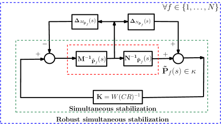
Figure 2: Concept of robust simultaneous stabilization

Lemma III.1.

Let $W$ and $R$ are chosen for achieving the desired decoupling. Then, the output feedback controller, $\mathbf{K}=W(CR)^{-1}$, of $\mathbf{\tilde{P}}_{cp}(s)$ accomplishes robust simultaneous stabilization of N plants belonging to $\xi=\big{\{}\mathbf{\tilde{P}}(s)\leavevmode\nobreak\ \big{|}\leavevmode\nobreak\ \mathbf{\tilde{P}}(s)\in\kappa,\delta_{v}(\mathbf{\tilde{P}}_{cp}(j\omega),\mathbf{\tilde{P}}(j\omega))\leq\bar{J}_{1}\leavevmode\nobreak\ \mathbf{\tilde{P}}_{cp}(s)\in\kappa\big{\}}$ and provides exact desired decoupling to the CL plant of $\mathbf{\tilde{P}}_{cp}(s)$, if the following conditions are satisfied.

1. $\lambda_{l}$ $\in$ $S_{1}$ $\forall$ $l$ $\in$ {1,2,…,$\hat{r}$}

2. $\lambda_{i}$ $\in$ $S_{1}$ $\forall$ $i$ $\in$ {$\hat{r}$+1,$\hat{r}$+2,…,n}

3. $b_{\mathbf{\tilde{P}}_{cp},\mathbf{K}}>\bar{J}_{1}$

Proof.

$\mathbf{K}$ stabilizes $\mathbf{\tilde{P}}_{cp}(s)$ when the conditions [1] and [2] are met. Concurrently, $\mathbf{K}$ provides exact desired decoupling to $\mathbf{\tilde{P}}_{cp}(s)$ and simultaneously stabilizes N plants belonging to $\xi$ when $\mathbf{K}$ achieves all three conditions. Now to prove $\mathbf{K}$ achieves robust simultaneous stabilization of N plants, let us define the ball of plants, $B(\mathbf{\tilde{P}}_{cp}(s),\bar{J}_{1})$, as

$$\begin{split}B(\mathbf{\tilde{P}}_{cp}(s),\bar{J}_{1})={}&\big{\{}\textrm{${\mathbf{\breve{P}}}(s)$ $\big{|}$ $\delta_{v}$\big{(}$\mathbf{\tilde{P}}_{cp}(j\omega)$, ${\mathbf{\breve{P}}}(j\omega)$\big{)} $\leq$ $\bar{J}_{1}$},\\ &\qquad\textrm{$\mathbf{\tilde{P}}_{cp}(s)$ $\in$ $\xi$, ${\mathbf{\breve{P}}}(s)$ $\in$ $\mathcal{RL_{\infty}}^{\hat{r}\times\hat{m}}$}\big{\}}\end{split}$$ (24)

When $\mathbf{K}$ satisfies all the three conditions, any plant belonging to $\partial B$ (boundary of $B(\mathbf{\tilde{P}}_{cp}(s),\bar{J}_{1})$) is also stabilized by $\mathbf{K}$ as $v-$gap metrics between the plants belonging to $\partial B$ and $\mathbf{\tilde{P}}_{cp}(s)$ are $\bar{J}_{1}$. $v-$gap metrics between $\mathbf{\tilde{P}}_{cp}(s)$ and the plants in $Int($B$)$ (interior of $B(\mathbf{\tilde{P}}_{cp}(s),\bar{J}_{1})$) are less than $\bar{J}_{1}$ as $\bar{J}_{1}$ is the maximum $v-$gap metric of $\mathbf{\tilde{P}}_{cp}(s)$. Therefore, $\mathbf{K}$ simultaneously stabilizes all the plants belong to $B(\mathbf{\tilde{P}}_{cp}(s),\bar{J}_{1})$ if the conditions [1], [2], and [3] are met. As $\xi$ $\subset$ $B(\mathbf{\tilde{P}}_{cp}(s),\bar{J}_{1})$, $\mathbf{K}$ simultaneously stabilizes all the N plants. Even if any plant, $\mathbf{\tilde{P}}(s)$ $\in$ $\xi$ is perturbed to form the plant, $\underline{\mathbf{P}}(s)$ $\in$ $B(\mathbf{\tilde{P}}_{cp}(s),\bar{J}_{1})\backslash\xi$ is also stabilized by $\mathbf{K}$. Therefore, $\mathbf{K}$ achieves robust simultaneous stabilization of N plants belonging to $\xi$. This establishes the proof. ∎

The three conditions of Lemma III.1 imply sufficient conditions for the existence of a RSSD output feedback controller. Moreover, the structure of $\xi$ suggests any $\mathbf{K}$ that satisfies the three conditions of Lemma III.1 also achieves robust simultaneous stabilization of N plants of $\mathcal{P}$.

III-D NN-RSSD Algorithm

An iterative algorithm is required for solving a RSSD problem due to the NP-hard nature of output feedback and SS problems. The controller generated by the iterative algorithm becomes the solution of a RSSD problem once this controller satisfies three conditions of Lemma III.1. Using these conditions, we now recast a RSSD problem as an optimization problem that is given as

$$\underset{\mathbf{K}}{\text{minimize}} J_{2}=\bigg{|}\bigg{|}\left[\begin{array}[]{c}{\mathbf{\tilde{P}}_{cp}(s)}\\ {\mathbf{I}}\end{array}\right]\left(\begin{array}[]{c}{\mathbf{I-K\tilde{P}}_{cp}(s)}\end{array}\right)^{-1}\left[\begin{array}[]{cc}{\mathbf{-I}}&{\mathbf{K}}\end{array}\right]\bigg{|}\bigg{|}_{\infty}$$ (25)

s.t. $$\lambda_{l} \in S_{1} \forall l \in \hat{r}$$ {1,2,…,}

$$\mathbf{K}=W(CR)^{-1}$$

$$\lambda_{i} \in S_{1} \forall i \in \hat{r} \hat{r}$$ {+1,+2,…,n}

The solution of a RSSD problem is a $\mathbf{K}\in\mathbb{R}^{\hat{m}\times\hat{r}}$ that reduces $J_{2}$ below $\bar{J}_{1}$ with all the constraints of (25) satisfied. A genetic algorithm based offline iterative algorithm referred to as the NN-RSSD algorithm is developed for sequentially solving the optimization problems associated with the SCP problem and the RSSD problem. The genetic algorithm is employed in the iterative algorithm as the optimization problem associated with the SCP problem is non-convex and non-smooth. At first, the NN-RSSD algorithm solves the optimization problem of the SCP problem given in (12). Then, the optimization problem of the RSSD problem given in (25) is solved utilizing the solution of the SCP problem. For this purpose, the NN-RSSD algorithm has two population-based genetic algorithm (GA) solvers, namely, GA-SCP and GA-RSSD. GA-SCP solves the optimization problem of the SCP problem, whereas GA-RSSD solves the optimization problem of the RSSD problem. In GA-SCP and GA-RSSD, GA employs the following steps.

1. Randomly generate initial values of search variables.

2. Compute the value of fitness function using the feasible values among the values of search variables.

3. Generate new values of search variables by examining the fitness value of search variables and applying genetic operators on the values of search variables.

4. Repeat 2 and 3 until the stopping criterion is satisfied.

Search Variables: The search variables of GA-SCP are the coefficients of $\mathbf{W_{ot}}(s)$ and $\mathbf{W_{in}}(s)$. The feasible values of these search variables are those which satisfy all the constraints of the problem given in (12). In the NN-RSSD algorithm, the chosen desired eigenvector element for mode decoupling is not assigned a zero value, but it is confined in a bounded set and used as a search variable by GA-RSSD. This reduces the failure of the eigenstructure assignment algorithm in computing the controller gain using (15) when all the chosen desired eigenvector elements are assigned with zero value. Further, the availability of the chosen desired eigenvector element as search variables contributes additional freedom in the computation of the controller defined by (15). The bound on a chosen desired eigenvector element is determined by the magnitude of unfavorable dominance of a mode on the state variable. Also, the search variables of GA-RSSD include $\hat{r}$ desired CL eigenvalues. The feasible values of $\hat{r}$ eigenvalues and chosen desired eigenvectors are those belonging to $S_{1}$ and the user-defined bounded set, respectively.

Fitness functions: The fitness function of GA-SCP is the performance index, $J_{1}$, of the optimization problem given in (12). The fitness function of GA-RSSD is the performance index, $J_{2}$, of the optimization problem given in (25).

Termination Conditions: The NN-RSSD algorithm terminates when the number of generation of GA-SCP exceeds its maximum value or when GA-RSSD generates a feasible RSSD output feedback controller.

The working of the NN-RSSD algorithm is explained as follows. At first, GA randomly obtains the initial values of the search variables of GA-SCP. Then, the fitness function of GA-SCP is evaluated, as shown in Algorithm-1. During this fitness evaluation, if the obtained solution satisfies an adaptive constraint, then the GA-SCP invokes GA-RSSD and passes $\mathbf{\tilde{P}}_{cp}(s)$ and its maximum $v-$gap metric to the GA-RSSD. The adaptive constraint employed here is fitness value of GA-SCP $<$ $\bar{J}_{1}$. During the fitness function evaluation of the GA-RSSD, if the value of the fitness function satisfies the condition, $J_{2}<\frac{1}{\bar{J}_{1}}$, then that controller becomes the feasible controller. Thereafter, the NN-RSSD algorithm terminates. When the GA-RSSD could not find a feasible controller for a $\mathbf{\tilde{P}}_{cp}(s)$, then $\bar{J}_{1}$ is assigned with the fitness value that previously satisfied the adaptive constraint. Note that, new $\bar{J}_{1}$ $<$ old $\bar{J}_{1}$ enables GA-SCP to search for newer $\mathbf{\tilde{P}}_{cp}(s)$ that has a maximum $v-$gap metric which is less than new $\bar{J}_{1}$. This enhances the possibility of obtaining a feasible RSSD output feedback controller. During the fitness evaluation of GA-SCP, if the solution obtained does not satisfy an adaptive constraint, then GA searches for new feasible values. Note that for computing $\mathbf{K}$ requires the inverse of $CR$. If the condition number of $CR$, $\kappa(CR)$, is infinity, then $CR$ singular. Following this, the existence of the inverse of $CR$ is guaranteed by satisfying the condition, $\kappa(CR)<10^{5}$. If this condition is satisfied, then compute $\mathbf{K}=W(CR)^{-1}$ else GA obtain new feasible values of GA-RSSD’s search variables. The pseudocode of the NN-RSSD algorithm is given in Algorithm-1 and Algorithm-2.

IV Design and Performance Evaluation of the RSSD Output Feedback Controller for a Fixed-Wing NAV

This section discusses the design of a RSSD output feedback controller using the NN-RSSD algorithm for eight unstable MIMO adversely coupled plants of the NAV mentioned in [3]. More details about the nonlinear and linear plants of the NAV, desired eigenvector elements, and bounds of pre/post compensators are given in the supporting material. Among the output variables of these plants (pitch angle ($\theta$), pitch rate ($q$), yaw rate ($r$), roll rate ($p$), and roll angle ($\phi$)), the controlled variables are $\theta$ and $\phi$. The frequency characteristics of the eight plants require modifications as they do not have the desired characteristics. To incorporate necessary frequency characteristics on the output sensitivity function, we require $\mathbf{W_{ot}}(s)$ and $\mathbf{W_{in}}(s)$ that satisfy $\underline{\sigma}(\mathbf{W_{ot}(0)}\mathbf{P}_{f}(0)\mathbf{W_{in}(0)})>\leavevmode\nobreak\ 6$ dB and $\underline{\sigma}(\mathbf{W_{ot}}(j\omega)\mathbf{P}_{f}(j\omega)\mathbf{W_{in}}(j\omega))\leavevmode\nobreak\ >\leavevmode\nobreak\ 0$ dB up to the desired frequency for all $f\in\{1,2,\dots,8\}$. Here, the desired frequency ranges from 15.28 rad/s to 53.3 rad/s. $\mathbf{P}_{2}(s)$ among the eight plants is identified as the central plant as it has the smallest maximum $v-$gap metric of 0.4489 ($\min\leavevmode\nobreak\ \bar{\epsilon}$).

Algorithm 1 Pseudocode of NN-Algorithm

1:Input: $\mathcal{P}$, $\bar{J}_{1}$, $n$, and $\hat{r}$

2:if number of generation of GA-SCP$\leq$ maximum value then

3:     GA obtain feasible values of GA-SCP’s search variables

4:     Compute: $\mathbf{W_{in}}(s)$ and $\mathbf{W_{ot}}(s)$ using (13)-(16) given in [24].

5:     Compute: $J_{1}$ for fitness evaluation

6:     if Fitness value $<$ $\bar{J}_{1}$ then

7:         Obtain: $\mathbf{\tilde{P}}_{cp}(s)$ by performing $v-$gap metric analysis on $\xi$

8:         Set $\bar{J}_{1}$=Fitness value

9:         GA-RSSD($\mathbf{\tilde{P}}_{cp}(s)$, $\bar{J}_{1}$, $n$, $\hat{r}$)

10:         go to 2

11:     else

12:         go to 2

13:     end if

14:else

15:     Exit

16:end if

Algorithm 2 Pseudocode of GA-RSSD

1:function GA-RSSD($\mathbf{\tilde{P}}_{cp}(s)$, $\bar{J}_{1}$, $n$, $\hat{r}$)

2:     if number of generation of GA-RSSD$\leq$ maximum value then

3:         GA obtain feasible values of GA-RSSD’s search variables

4:         Compute: $W$ and $R$ (using $A$ and $B$ of $\mathbf{\tilde{P}}_{cp}(s)$ and feasible values of search variables of GA-RSSD)

5:         Compute: $CR$ and $\kappa(CR)$

6:         if  $\kappa(CR)$ $<$ 10⁵ then

7:              Compute: $\mathbf{K}=W(CR)^{-1}$

8:              if $\lambda_{i}(A+B\mathbf{K}C)\leavevmode\nobreak\ \forall\leavevmode\nobreak\ i\in\{1,2,\dots,n\}\in S_{1}$ then

9:                  Compute: $J_{2}$ for fitness evaluation

10:                  if Fitness value $<$ $\frac{1}{\bar{J}_{1}}$ then

11:                       Controller found ($\mathbf{K}$) and Exit

12:                  else

13:                       go to 2

14:                  end if

15:              else

16:                  go to 2

17:              end if

18:         else

19:              go to 2

20:         end if

21:     else

22:         return

23:     end if

24:end function

IV-A Flight Control System Design Specifications and Controller Gain Synthesis

1. Damping Ratio Specifications: The minimum required damping ratios for all the oscillatory modes of the NAV are taken as 0.30.

2. Tracking Specifications: The tracking error in the pitch angle and the roll angle of the NAV in the absence of wind disturbances concerning the reference signal are ${\pm 0.0087}$ rad and ${\pm 0.0175}$ rad, respectively. Also, in the presence of wind disturbances, root mean square deviation (RMS) of the pitch angle and roll angle need not exceed 0.0873 rad and 0.175 rad, respectively.

3. Robustness Requirements: An uncertainty level of 40 $\%$ is assigned to all the static, dynamic, and control derivatives of the NAV. Concurrently, for each CL plant, the controller has to provide a multiloop disk-based gain margin (MDGM) and phase margin (MDPM) of $\pm$3 dB and $\pm$20 deg, respectively.

4. Desired eigenvalues and eigenvectors: The eigenvalues of the coupled spiral, coupled Dutch roll, and coupled short period modes of the NAV are assigned as these eigenvalues do not possess the desired stability and performance characteristics. For more details about these modes and their coupling characteristics, one should refer [3]. The bounds on the chosen desired eigenvector elements for mode decoupling are given in Table I. In Table I, $\bar{u}$, $\bar{w}$, $\bar{r}$, $\bar{p}$, and $\bar{\phi}$ denote the eigenvector elements associated with the state variables, $u$ (translational velocity in $\mathbf{x}$ body-axis), $w$ (translational velocity in $\mathbf{w}$ body-axis), $r$, $p$, and $\phi$, respectively.

Table I: Bounds on the chosen desired eigenvector elements

Mode	Eigenvector	Bound
	Element
Coupled Spiral	$\bar{u},\bar{w},\bar{r}$	$\pm$0.01, $\pm$0.01,$\pm$0.01
Coupled Dutch	$\bar{p}$	[$\pm$0.049]$\pm$[$\pm$0.049]$j$
roll	$\bar{\phi}$	[$\pm$0.1]$\pm$[$\pm$0.08]$j$
Coupled Short	$\bar{r}$	[$\pm$0.015]$\pm$[$\pm$0.15]$j$
period

The NN-RSSD algorithm is executed with inputs, $\hat{r}=5$, $\hat{m}=3$, $n=19$, $\bar{J}_{1}$=0.4489, $\mathcal{P}$, the bounds on the coefficients of $\mathbf{W_{ot}}(s)$ and $\mathbf{W_{in}}(s)$, the bounds on the chosen desired eigenvector elements, the maximum number of generations of GA-SCP (20) and GA-RSSD (1000), and $S_{1}$ defined for the damping ratio of 0.3. NN-RSSD algorithm terminates at the 388th generation of GA-RSSD. Subsequently, the feasible compensators are given as

$$\mathbf{W_{in}}(s)=diag\bigg{[}\frac{1.0s+7.36}{0.007s+10.1},\frac{14.71s+59.78}{0.002s+0.099},\frac{0.992s+5.091}{0.0053s+11.89}\bigg{]}$$ (26)

$$\begin{split}\mathbf{W_{ot}}(s)={}&diag\bigg{[}\frac{0.61s+11}{1.6s+1.6},\frac{0.23s+29.58}{0.55s+0.36},\frac{0.813s+12.1}{7.996s+1.46},\\ &\qquad\frac{0.91s+9.78}{0.331s+0.342},\frac{0.78s+16.81}{1.41s+1.0}\bigg{]}\end{split}$$ (27)

The feasible RSSD output feedback controller gain is given as

$$\small{\mathbf{K}=\left[\begin{array}[]{ccccc}{1.13}&{0.78}&{0.26}&{0.14}&{0.13}\\ {-1.07}&{-0.78}&{0.74}&{0.009}&{0.54}\\ {0.19}&{-0.06}&{-0.002}&{1.29}&{0.04}\end{array}\right]}$$ (28)

Besides this, the SCP central plant is $\mathbf{\tilde{P}}_{cp}(s)$=$\mathbf{W_{ot}}(s)\mathbf{P}_{3}(s)\mathbf{W_{in}}(s)$ with the maximum $v-$gap metric of 0.3184. As this value is less than 0.4489, one of the objectives of the pre and post compensators is achieved. The frequency characteristics of $\mathbf{\tilde{P}}_{f}(s)$ = $\mathbf{W_{ot}}(s)\mathbf{P}_{f}(s)\mathbf{W_{in}}(s)$ for all $f\in\{1,2,\dots,8\}$ are shown in Fig. 3.

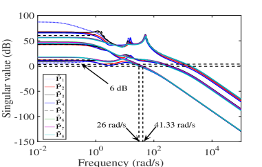
Figure 3: Singular value plots of the plants

.

This figure indicates $\underline{\sigma}(\mathbf{\tilde{P}}_{f}(0))>6$ dB for all $f\in\{1,2,\dots,8\}$. As illustrated in Fig. 3, the 0 dB crossing frequencies of all the performance enhanced plants are within the desired limit as the range of 0 dB crossing frequencies of $\underline{\sigma}(\mathbf{\tilde{P}}_{f}(s))$ for all $f\in\{1,2,\dots,8\}$ are within 26-41.33 rad/s. Hence, $\mathbf{W_{in}}(s)$ and $\mathbf{W_{ot}}(s)$ given in (26) and (27) satisfy all the design requirements with respect to the performance enhanced plants.

IV-B Stability analysis

The controller gain given in (28) simultaneously stabilizes eight plants of the NAV as all the eigenvalues of the CL plants, $\mathbf{\hat{H}}_{f}(s)=\frac{\mathbf{\tilde{P}}_{f}(s)\mathbf{K}}{\mathbf{I}-\mathbf{\tilde{P}}_{f}(s)\mathbf{K}}$ for all $f\in\{1,2,\dots,8\}$ lie in $\mathcal{C}_{-}$ as shown in Fig. 4.

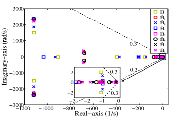
Figure 4: Eigenvalues of the closed-loop plants of NAV

This figure also indicates the damping ratios of all the CL eigenvalues are greater than or equal to 0.3. Besides this, Table II suggest that all the eight CL plants have desired MDGM and MDPM.

Table II: Multiloop disk-based gain (dB) and phase margins (deg) of the NAV

Plant	MDGM	MDPM	Plant	MDGM	MDPM
$\mathbf{\hat{H}_{1}}(s)$	$\pm$4.30	$\pm$27.30	$\mathbf{\hat{H}_{5}}(s)$	$\pm$3.39	$\pm$21.79
$\mathbf{\hat{H}_{2}}(s)$	$\pm$3.42	$\pm$22.00	$\mathbf{\hat{H}_{6}}(s)$	$\pm$3.37	$\pm$21.69
$\mathbf{\hat{H}_{3}}(s)$	$\pm$3.88	$\pm$24.87	$\mathbf{\hat{H}_{7}}(s)$	$\pm$3.44	$\pm$22.10
$\mathbf{\hat{H}_{4}}(s)$	$\pm$3.33	$\pm$21.44	$\mathbf{\hat{H}_{8}}(s)$	$\pm$3.50	$\pm$22.51

The parametric and unmodeled dynamic uncertainties are represented by the inverse input multiplicative and output multiplicative uncertainties, respectively. The tolerance level of the CL plants against the output multiplicative uncertainty is analyzed using the plots of $\frac{1}{\overline{\sigma}(\mathbf{\tilde{P}}_{f}(j\omega)\mathbf{K}(\mathbf{I-\tilde{P}}_{f}(j\omega)\mathbf{K})^{-1})}$ for all $f\in\{1,2,\dots,8\}$ depicted in Fig. 5. This figure depicts that the output multiplicative uncertainty tolerance levels increase with the frequency. This characteristic is required to tackle the output multiplicative uncertainty that occurs in the high-frequency region. Further, $\mathbf{\hat{H}}_{3}(s)$ has the worst-case tolerance level of about 51.8 $\%$ at 2.22 rad/s. This tolerance level is in the low-frequency region (with respect to the bandwidth of the augmented plants), where the unmodeled dynamic uncertainty does not occur. The tolerance level of the CL plant against the inverse input multiplicative uncertainty is analyzed by studying the plots of $\frac{1}{\overline{\sigma}(\mathbf{(I-K}\mathbf{\tilde{P}}_{f}(s))^{-1})}$ for all $f\in\{1,2,\dots,8\}$ shown in Fig. 6. This figure shows $\mathbf{\hat{H}}_{4}(s)$ has the worst-case inverse input multiplicative uncertainty tolerance level of 62 $\%$ at 2987 rad/s. This worst-case tolerance level occurs in the high-frequency region, where parametric uncertainty does not exist. The tolerance levels of all the CL plants are greater than 79 $\%$ when the frequency is below 41.33 rad/s (maximum bandwidth of augmented plant). This satisfies the tolerance level requirement against the parametric uncertainties.

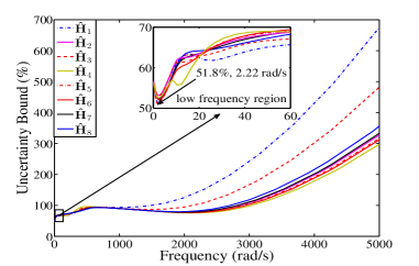
Figure 5: Output multiplicative uncertainty bound

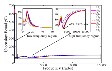
Figure 6: Inverse input multiplicative uncertainty bound

IV-C Performance and decoupling analysis

The performance of the controller is evaluated by analyzing the singular value plots of output sensitivity function, $\mathbf{S_{o}}_{f}(s)=\mathbf{(I-\tilde{P}}_{f}(s)\mathbf{K)}^{-1}$ shown in Fig. 7. The controller rejects any disturbance with a frequency less than 197 rad/s acting on any controllable output channels of the NAV as Fig. 7 indicates worst 0 dB crossing frequency (from below) of $\overline{\sigma}(\mathbf{S_{o}}_{f}(j\omega))$ at the controllable output channel is 197 rad/s. The worst magnitudes of $\overline{\sigma}(\mathbf{S_{o}}_{f}(0))$ associated with $\bar{r}$, $\bar{\phi}$, and $\bar{\theta}$ output channels are -7.8 dB, -44.6 dB, and -59.8 dB, respectively. Hence, the worst maximum steady-state error for a step input at the controllable output channels are 40.7 $\%$, 0.6 $\%$, and 0.01 $\%$, respectively. The detailed performance analysis including the input sensitivity, $\mathbf{S_{I}}_{f}(s)$ and $\mathbf{KS_{o}}_{f}(s)$ are given in the supporting material. The value of chosen desired eigenvector elements associated with the coupled spiral mode of CL plant of $\mathbf{\tilde{P}}_{cp}(s)$ are $\bar{u}$=-0.0065, $\bar{w}$=0.0905, and $\bar{r}$=-0.0002. For the coupled Dutch roll mode, the value of these elements are $\bar{p}$=-0.0159$\pm$0.0423$j$ and $\bar{\phi}$=-0.0010$\pm$0.0039$j$. Likewise, the chosen desired eigenvector element of coupled short period mode is $\bar{r}$=-0.0003$\pm$0.0001$j$. The values of these elements suggest that they are within the bounds given in Table I.

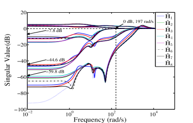
Figure 7: Singular value plots of the output sensitivity functions

IV-D Six-Degree-of-Freedom Simulations

To assess the performance of the controller, five cases of six-degree-of-freedom simulations are accomplished. In first and second cases of simulations, the CL nonlinear and linear plants of the NAV are forced to track a doublet $\theta$ and $\phi$ reference signals separately. The block diagram of the system structure for the simulation of CL nonlinear dynamics of the NAV is given in supporting material. The magnitude and pulse width of the doublet $\theta$ reference signal are ${\pm 0.0873}$ rad (${\pm 5}$ deg) and 2 s, respectively. Similarly, the doublet $\phi$ reference signal has a magnitude of ${\pm 0.0349}$ rad (${\pm 2}$ deg) and a pulse width of 2 s. The output time responses of the linear CL plant of $\mathbf{\tilde{P}}_{cp}(s)$ offsetted with the trim values are shown in Figs. 8(b)-9(e) along with the output time responses of the corresponding nonlinear CL plant. The output time responses of all the CL plants are given in the supporting material. After analyzing all these plots, the following conclusions are made.

1. The CL nonlinear plants are stable as their time responses of output variables are not diverging in finite time. The time responses of the CL nonlinear and linear (with offset) plants are almost identical, which establishes that the linear plant accurately captures the behavior of the nonlinear plant around the trim point. Furthermore, the CL plants are tracking their reference signals as the tracking variables are within the specified error band.

2. While tracking the doublet $\theta$ reference signal, the change in yaw rate responses is minimal when compared to the roll rate and pitch rate responses. This indicates that the coupled short period mode of all the CL plants are decoupled from yaw rate response which is one of the design requirement.

3. Compared to the change in yaw rate responses, a substantial change in roll rate responses are visible when all the CL plants track the doublet $\theta$ command. This large change is mainly due to the variation of counter torque due to the change in $\delta_{T}$ and thereby thrust. The coupling induced by counter torque affects the coupled roll modes of all the CL plants and thereby the roll rates. The controller is not designed to decouple the coupled roll modes from roll rate responses, which result in the excitation of the roll rates when the NAV is forced to track a doublet $\theta$ command. However, the converging (converging to the trim value) of roll rate responses establishes that the coupled roll modes of all the CL plants are stable. The roll angle responses indicate the variations in the roll angle responses are minimal. This is because the effect of counter torque on the coupled spiral mode is minimal as $u$ and $w$ are decoupled from the coupled spiral mode. Furthermore, the time responses indicate that all the CL plants have similar desired decoupling characteristics and thus, the controller accomplishes one of the design objectives.

In the third case and the fourth case, the effectiveness of the controller in tolerating the parametric and unmodeled dynamic uncertainties is evaluated. To evaluate the effect of parametric uncertainty, 40 $\%$ of uncertainty is induced in the static, dynamic, and control derivatives of the NAV by multiplying these derivatives with the signal (with the frequency of 25.13 rad/s) shown in Fig. 8(a) while nonlinear CL plant of $\mathbf{\tilde{P}}_{cp}(s)$ tracks a doublet $\theta$ reference signal. Likewise, to evaluate the effect of unmodeled dynamic uncertainty, an unmodeled dynamic uncertainty is modeled by adding the frequency-dependent weight, $G(s)=\frac{3s+923.9}{s+9239}$, to the closed-loop (as shown in the Fig. 8 of the supporting material). This weight induces 50 $\%$ relative uncertainty up to 60 rad/s to the respective output channel. The relative uncertainty rising thereafter induces 100$\%$ relative uncertainty at 3250 rad/s. Corresponding simulation results indicate that the CL nonlinear plant is stable, as the output responses are not diverging as shown in Figs. 8(b)-9(e). Additionally, the CL nonlinear plant is tracking its reference signal. The effectiveness of the controller in attenuating the disturbance is tested in the fifth case of simulation. Moreover, the hardware-in-loop simulations (HILS) of the CL nonlinear plants of the NAV are also accomplished. The details of both these simulation results are given in supporting material. The video of HILS can be found in https://youtu.be/UCscRGwaNqI.

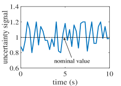
(a) Uncertainty signal

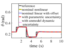
(b) Pitch angle response

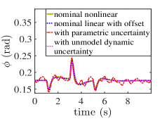
(c) Roll angle response

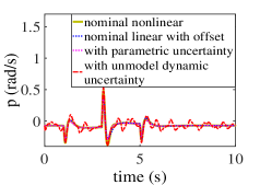
(d) Roll rate response

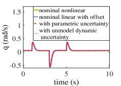
(e) Pitch rate response

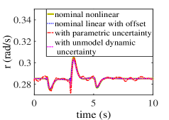
(f) Yaw rate response

Figure 8: $\theta$ tracking performance of CL plant of $\mathbf{\tilde{P}}_{cp}(s)$

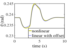
(a) Pitch angle response

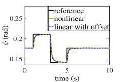
(b) Roll angle response

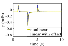
(c) Roll rate response

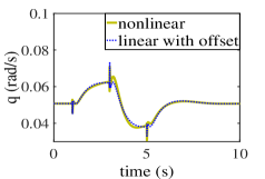
(d) Pitch rate response

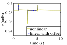
(e) Yaw rate response

Figure 9: $\phi$ tracking performance of CL plant of $\mathbf{\tilde{P}}_{cp}(s)$

V Conclusions

A new tractable method based on the central plant is developed to synthesize a RSSD output feedback controller for a finite set of unstable MIMO adversely coupled plants of a NAV having resource-constrained autopilot hardware. To this end, the method developed to identify the central plant is tractable and is suitable for stable/unstable plants with the varying/same number of unstable poles. The sufficient conditions for the existence of the RSSD output feedback controller developed are easily testable for a given set of plants. Further, the tractability of the method developed using these conditions to solve the RSSD problem is successfully demonstrated by generating a feasible RSSD output feedback controller for the eight unstable plants of the fixed-wing NAV. All the CL plants with this controller demonstrate that they satisfy desired design specifications as indicated by the stability, performance, and decoupling analyzes and the six-degree-of-freedom simulation results. Additionally, the hardware-in-the-loop simulation results show that there are no implementation issues associated with the controller and the compensators.

Jinraj V Pushpangathan received his Ph.D. degree in aerospace engineering from Indian Institute of Science (IISc), India in 2018. Currently, he is working as research fellow in Aerospace Department of IISc. His research interests are robust and optimal control theory, guidance and control of unmanned systems, and flight dynamics and control.

K. Harikumar is currently an Assistant Professor in International Institute of Information Technology, Hyderabad, India. He received the Ph.D. degree in aerospace engineering from the Indian Institute of Science (IISc), India in 2015. His research interests are applications of control theory to unmanned systems and flight dynamics.

Suresh Sundaram (SM’08) received the Ph.D. degrees in aerospace engineering from the Indian Institute of Science (IISc), India, in 2005, where he is currently an Associate Professor. From 2010-2018, he was an Associate Professor with the School of Computer Science and Engineering, Nanyang Technological University. His current research interests include machine learning, optimization, and computer vision.

Narasimhan Sundararajan (LF’11) received the Ph.D. degree in electrical engineering from the University of Illinois at Urbana-Champaign, Urbana, IL, USA, in 1971. From 1971 to 1991, he was with the Vikram Sarabhai Space Centre, Indian Space Research Organization, Trivandrum, India. From 1991, he was a Professor (Retd.) with the School of Electrical and Electronic Engineering, Nanyang Technological University (NTU), Singapore. He was a Senior Research Fellow with the School of Computer Engineering, NTU. His current research interests include spiking neural networks, neuro-fuzzy systems, and optimization with swarm intelligence.

References

- [1] L. Petricca, P. Ohlckers, and C. Grinde, “Micro- and Nano-Air Vehicles: State of the Art,” International Journal of Aerospace Engineering, vol. 2011, Article ID 214549, 2011.
- [2] I. Kaminer, A. Pascoal, E. Hallberg and C. Silvestre, ”Trajectory Tracking for Autonomous Vehicles: An Integrated Approach to Guidance and Control ,” Journal of Guidance Control and Dynamics, vol. 21, no. 1, pp. 29-38 , Jan.-Feb. 1998.
- [3] J. V. Pushpangathan, M. S. Bhat, and K. Harikumar, “Effects of Gyroscopic Coupling and Countertorque in a Fixed-Wing Nano Air Vehicle,” Journal of Aircraft, vol. 55, no.1, pp. 239-250, Jan.-Feb. 2018.
- [4] F. Santoso, M. A. Garratt, S. G. Anavatti, and I. Petersen, ”Robust Hybrid Nonlinear Control Systems for the Dynamics of a Quadcopter Drone,” IEEE Trans. Syst., Man, Cybern., Syst., vol. 50, no. 8, pp. 3059-3071, Aug. 2020.
- [5] F. Santoso, M. A. Garratt, and S. G. Anavatti, ”Hybrid PD-Fuzzy and PD Controllers for Trajectory Tracking of a Quadrotor Unmanned Aerial Vehicle: Autopilot Designs and Real-Time Flight Tests,” IEEE Trans. Syst., Man, Cybern., Syst., [online], April 2019, DOI: 10.1109/TSMC.2019.2906320
- [6] W. He , T Meng , S. Zhang, Q. Ge, and C . Sun, ”Trajectory Tracking Control for the Flexible Wings of a Micro Aerial Vehicle,” IEEE Trans. Syst., Man, Cybern., Syst., vol. 48, no. 12, pp. 2431-2441, Dec. 2018.
- [7] K. Harikumar, S. Dhall, and M. S. Bhat, “Nonlinear Modeling and Control of Coupled Dynamics of a Fixed Wing Micro Air Vehicle,” 2016 Indian Contr. Conf. (ICC), Hyderabad, India, 2016, pp. 318-323.
- [8] C. Langbort, R. S.Chandra, and R. D’Andrea, “Distributed Control Design for Systems Interconnected Over an Arbitrary Graph,” IEEE Trans. Automat. Contr., vol. 49, no. 9, pp. 1502-1519, Sept. 2004.
- [9] W. Zhou, K. Yin, R. Wang, and Y. Wang, “ Design of Attitude Control System for UAV Based on Feedback Linearization and Adaptive Control,” Mathematical Problems in Engineering, vol. 2014, Article ID 492680, 2014.
- [10] T. Espinoza, A. E. Dzul, R. Lozano, and P. Parada, ”Backstepping - Sliding Mode Controllers Applied to a Fixed-Wing UAV,” Journal of Intelligent and Robotic Systems, vol. 73, no. 1-4, pp. 67-69, 2014.
- [11] S. Suresh, S. N. Omkar, V. Mani, and N. Sundararajan, ”Nonlinear Adaptive Neural Controller for Unstable Aircraft,” Journal of Guidance Control and Dynamics, vol. 28, no. 6, pp. 1103-1111, Nov.-Dec. 2005.
- [12] J. V. Pushpangathan, “Design and Development of 75 mm Fixed-Wing Nano Air Vehicle,” Ph.D. dissertation, Dept. Aero. Eng., Indian Institute of Science, Bangalore, India, 2017.
- [13] R. Saeks, and J. Murray, ”Fractional Representation, Algebraic Geometry, and the Simultaneous Stabilization Problem,” IEEE Trans. Automat. Contr., vol. AC-27, no. 4, pp. 895-903, Aug. 1982.
- [14] M. Vidyasagar, and N. Viswanadham, ”Algebraic Design Techniques for Reliable Stabilization,” IEEE Trans. Automat. Contr., vol. 27, no. 5, pp. 1085-1095, Oct. 1982.
- [15] V. Blondel, and M. Gevers, ”Simultaneous Stabilizability of Three Linear Systems is Rationally Undecidable,” Mathematics of Control, Signals and Systems, vol. 6, no. 2, pp. 135-145, June 1993.
- [16] M. Toker, and H. Ozbay, ”On the NP-hardness of Solving Bilinear Matrix Inequalities and Simultaneous Stabilization with Static Output Feedback,” Proc. Amer. Control Conf., Seattle, WA, USA, 1995, pp. 2525-2526.
- [17] Y. Cao, Y. Sun, and J. Lam, ”Simultaneous Stabilization via Static Output Feedback and State Feedback,” IEEE Trans. Automat. Contr., vol. 44, no. 6, pp. 1277-1282, June 1999.
- [18] R. E. Perez, H. T. H. Liu, and K. Behdinan, ”Decomposition-Based Simultaneous Stabilization with Optimal Control,” Journal of Guidance, Control, and Dynamics, vol. 31, no. 3, pp. 647-655, May-June 2008.
- [19] D. N. Wu, W. B. Gao, and M. Chen, ”Algorithm for Simultaneous Stabilization of Single-Input Systems Via Dynamic Feedback,” Int. J. Contr., vol. 51, no. 3, pp. 631-642, 1990.
- [20] G. D. Howitt and R. Luus, ”Simultaneous Stabilization of Linear Single Input Systems by Linear State Feedback Control,” Int. J. Contr., vol. 54, no. 4, pp. 1058-1072, 1991.
- [21] J. C. Geromel, P. L. D. Peres, and J. Bernussou, ”On a Convex Parameter Space Method for Linear Control Design of Uncertain Systems,” SIAM J. Contr. Optim., vol. 29, no. 2, pp. 381-402, 1991.
- [22] M. Paskota, V. Sreeram, K. L. Teo, and A. I. Mees, ”Optimal Simultaneous Stabilization of Linear Single-Input Systems Via Linear State Feedback Control,” Int. J. Contr., vol. 60, no. 4, pp. 483-498, 1994.
- [23] A. Saif, D. Gu, and D. Kavranoglu, and I. Postlethwaite, ”Simultaneous Stabilization of MIMO Systems Via Robustly Stabilizing a Central Plant,” IEEE Trans. Automat. Contr., vol. 27, no. 2, pp. 363-369, Feb. 2002.
- [24] J. V. Pushpangathan, M. S. Bhat, and H. Kandath, ”v-Gap Metric–Based Simultaneous Frequency-Shaping Stabilization for Unstable Multi-Input Multi-Output Plants,” Journal of Guidance, Control, and Dynamics, vol. 41, no. 12, pp. 2687-2694, Dec. 2018.
- [25] J. Steele, and G. Vinnicombe, ”The Gap Metric and the Generalised Stability Margin” Advanced Techniques for Clearance of Flight Control Laws, edited by C. Fielding, A. Varga, S. Bennani, M. Selier, 1st edition, Springer, pp. 57-76, 2002.
- [26] G. Vinnicombe, Uncertainty and Feedback: Loop-shaping and the -gap Metric, London: Imperial College Press, 2001, pp. 104-165.
- [27] G. P. Liu, and R. J. Patton, Eigenstructure Assignment for Control System Design, USA, New York: John Wiley and Sons, 1998, pp. 9-28.