ASER: A Large-scale Eventuality Knowledge Graph

Abstract.

Understanding human’s language requires complex world knowledge. However, existing large-scale knowledge graphs mainly focus on knowledge about entities while ignoring knowledge about activities, states, or events, which are used to describe how entities or things act in the real world. To fill this gap, we develop ASER (activities, states, events, and their relations), a large-scale eventuality knowledge graph extracted from more than 11-billion-token unstructured textual data. ASER contains 15 relation types belonging to five categories, 194-million unique eventualities, and 64-million unique edges among them. Both intrinsic and extrinsic evaluations demonstrate the quality and effectiveness of ASER.

1. Introduction

In his conceptual semantics theory, Ray Jackendoff, a Rumelhart Prize winner, describes semantic meaning as ‘a finite set of mental primitives and a finite set of principles of mental combination (Jackendoff, 1990)’. The primitive units of semantic meanings include Thing (or Object), Activity, State, Event, Place, Path, Property, Amount, etc. Understanding the semantics related to the world requires the understanding of these units and their relations. Traditionally, linguists and domain experts built knowledge graphs (KGs) to formalize these units and enumerate categories (or senses) and relations of them. Typical KGs include WordNet (Fellbaum, 1998) for words, FrameNet (Baker et al., 1998) for events, and Cyc (Lenat and Guha, 1989) and ConceptNet  (Liu and Singh, 2004) for commonsense knowledge. However, their small scales restricted their usage in real-world applications.

Nowadays, with the growth of Web contents, computational power, and the availability of crowdsourcing platforms, many modern and large-scale KGs, such as Freebase (Bollacker et al., 2008), KnowItAll (Etzioni et al., 2004), TextRunner (Banko et al., 2007), YAGO (Suchanek et al., 2007), DBpedia (Auer et al., 2007), NELL (Carlson et al., 2010), Probase (Wu et al., 2012), and Google Knowledge Vault (Dong et al., 2014), have been built based on semi-automatic mechanisms. Most of these KGs are designed and constructed based on Things or Objects, such as instances and their concepts, named entities and their categories, as well as their properties and relations. On top of them, a lot of semantic understanding problems such as question answering (Berant et al., 2013) can be supported by grounding natural language texts on knowledge graphs, e.g., asking a bot for the nearest restaurants for lunch. Nevertheless, these KGs may fall short in circumstances that require not only knowledge about Things or Objects, but also those about Activities, States, and Events. Consider the following utterance that a human would talk to the bot: ‘I am hungry’, which may also imply one’s need for restaurant recommendation. This, however, will not be possible unless the bot is able to identify that the consequence of being hungry would be ‘having lunch’ at noon.

In this paper, we propose an approach to discovering useful real-world knowledge about Activities (or process, e.g., ‘I sleep’), States (e.g., ’I am hungry’), Events (e.g., ‘I make a call’), and their Relations (e.g., ‘I am hungry’ may result in ‘I have lunch’), for which we call ASER. In fact, Activities, States, and Events, which are expressed by verb-related clauses, are all eventualities following the commonly adopted terminology and categorization proposed by Mourelatos (P. D. Mourelatos, 1978) and Bach (Bach, 1986). While both activity and event are occurrences (actions) described by active verbs, a state is usually described by a stative verb and cannot be qualified as actions. The difference between an activity and an event is that an event is defined as an occurrence that is inherently countable (P. D. Mourelatos, 1978). For example, ‘The coffee machine brews a cup of coffee once more’ is an event because it admits a countable noun ‘a cup’ and cardinal count adverbials ‘once’, while ‘The coffee machine brews coffee’ is not an event with an imperfective aspect and it is not countable. Thus, ASER is essentially an eventuality-centric knowledge graph.

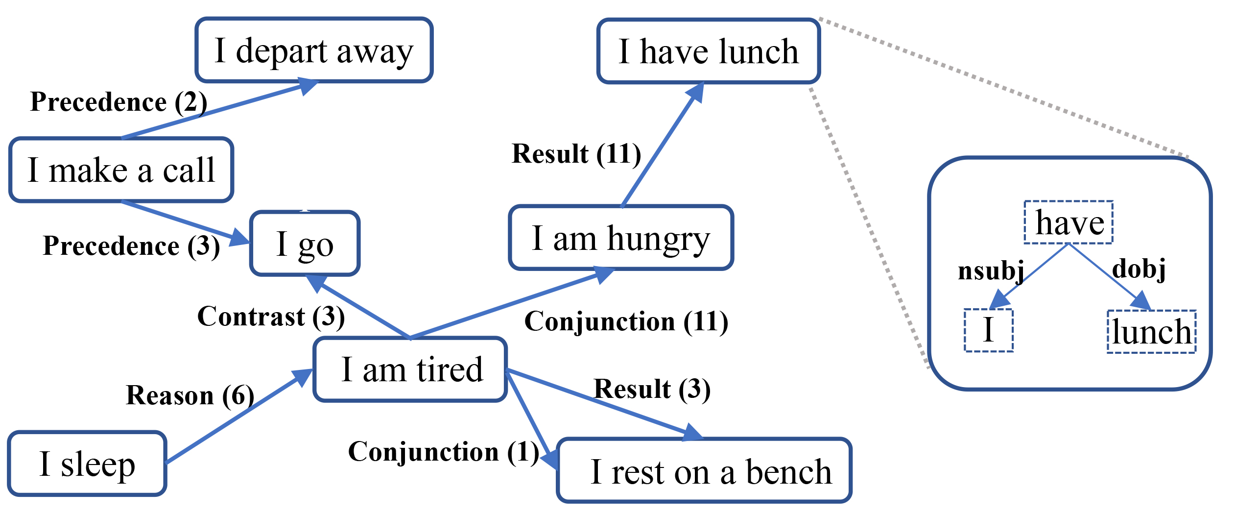
Figure 1. ASER Demonstration. Eventualities are connected with weighted directed edges. Each eventuality is a dependency graph.

For eventualities, traditional extraction approaches used in natural language processing based on FrameNet (Baker et al., 1998) or ACE (NIST, 2005) first define complex structures of events by enumerating triggers with senses and arguments with roles. They then learn from limited annotated examples and try to generalize to other text contents. However, detecting trigger senses and argument roles suffers from the ambiguity and variability of the semantic meanings of words. For example, using the ACE training data, the current state-of-the-art system can only achieve about 40% overall F1 score with 33 event types (Li et al., 2013). Different from them, we use patterns to extract eventuality-centric knowledge based on dependency grammar since the English language’s syntax is relatively fixed and consistent across domains and topics. Instead of defining complex triggers and role structures of events, we simply use syntactic patterns to extract all possible eventualities. We do not distinguish between semantic senses or categories of particular triggers or arguments in eventualities but treat all extracted words with their dependency relations as hyperedge in a graph to define an eventuality as a primitive semantic unit in our knowledge graph.

For eventuality relations, we use the definition linguistic shallow discourse relations used in Penn Discourse Treebank (PDTB) (Prasad et al., 2007). In PDTB, the relations are defined between two sentences or clauses. Simplified from PDTB, we focus on relations between two eventualities, which are defined with simple but semantically complete patterns. Moreover, as shown in PDTB, some connectives, e.g., ‘and’ and ‘but’, are less ambiguous than others, e.g., ‘while’. Thus, we use less ambiguous connectives as seed connectives to find initial relations and then bootstrap the eventuality relation extraction using large corpora. Although relations are extracted based on linguistic knowledge, we will show that they have correlations with previously defined commonsense knowledge in ConceptNet (Liu and Singh, 2004).

In total, ASER contains 194 million unique eventualities. After bootstrapping, ASER contains 64 million edges among eventualities. One example of ASER is shown in Figure 1. Table 1 provides a size comparison between ASER and existing eventuality-related (or simply verb-centric) knowledge bases. Essentially, they are not large enough as modern knowledge graph and inadequate for capturing the richness and complexity of eventualities and their relations. FrameNet (Baker et al., 1998) is considered the earliest knowledge base defining events and their relations. It provides annotations about relations among about 1,000 human defined eventuality frames, which contain 27,691 eventualities. However, given the fine-grained definition of frames, the scale of the annotations is limited. ACE (NIST, 2005) (and its follow-up evaluation TAC-KBP (Aguilar et al., 2014)) reduces the number of event types and annotates more examples in each of event types. PropBank (Palmer et al., 2005) and NomBank (Meyers et al., 2004) build frames over syntactic parse trees, and focus on annotating popular verbs and nouns. TimeBank focuses only on temporal relations between verbs (Pustejovsky et al., 2003). While the aforementioned knowledge bases are annotated by domain experts, ConceptNet (Liu and Singh, 2004), Event2Mind (Smith et al., 2018), ProPora (Dalvi et al., 2018), and ATOMIC (Sap et al., 2019) leveraged crowdsourcing platforms or the general public to annotate commonsense knowledge about eventualities, in particular the relations among them. Furthermore, KnowlyWood (Tandon et al., 2015) uses semantic parsing to extract activities (verb+object) from movie/TV scenes and novels to build four types of relations (parent, previous, next, similarity) between activities using inference rules. Compared with all these eventuality-related KGs, ASER is larger by one or more orders of magnitude in terms of the numbers of eventualities and relations it contains.

Table 1. Size comparison of ASER and existing eventuality-related resources. # Eventuality, # Relation, and # R types are the number of eventualities, relations between these eventualities, and relation types. For KGs containing knowledge about both entity and eventualities, we report the statistics about the eventualities subset. ASER (core) filters out eventualities that appear only once and thus has better accuracy while ASER (full) can cover more knowledge.

	# Eventuality	# Relation	# R Types
FrameNet (Baker et al., 1998)	27,691	1,709	7
ACE (Aguilar et al., 2014)	3,290	0	0
PropBank (Palmer et al., 2005)	112,917	0	0
NomBank (Meyers et al., 2004)	114,576	0	0
TimeBank (Pustejovsky et al., 2003)	7,571	8,242	1
ConceptNet (Liu and Singh, 2004)	74,989	116,097	4
Event2Mind (Smith et al., 2018)	24,716	57,097	3
ProPora (Dalvi et al., 2018)	2,406	16,269	1
ATOMIC (Sap et al., 2019)	309,515	877,108	9
Knowlywood (Tandon et al., 2015)	964,758	2,644,415	4
ASER (core)	27,565,673	10,361,178	15
ASER (full)	194,000,677	64,351,959	15

In summary, our contributions are as follows.

$\bullet$ Definition of ASER. We define a brand new KG where the primitive units of semantics are eventualities. We organize our KG as a relational graph of hyperedges. Each eventuality instance is a hyperedge connecting several vertices, which are words. A relation between two eventualities in our KG represents one of the 14 relation types defined in PDTB (Prasad et al., 2007) or a co-occurrence relation.

$\bullet$ Scalable Extraction of ASER. We perform eventuality extraction over large-scale corpora. We designed several high-quality patterns based on dependency parsing results and extract all eventualities that match these patterns. We use unambiguous connectives obtained from PDTB to find seed relations among eventualities. Then we leverage a neural bootstrapping framework to extract more relations from the unstructured textual data.

$\bullet$ Inference over ASER. We also provide several ways of inference over ASER. We show that both eventuality and relation retrieval over one-hop or multi-hop relations can be modeled as conditional probability inference problems.

$\bullet$ Evaluation and Applications of ASER. We conduct both intrinsic and extrinsic evaluations to validate the quality and effectiveness of ASER. For intrinsic evaluation, we sample instances of extracted knowledge in ASER over iterations, and submitted them to the Amazon Mechanical Turk (AMT) for human workers to verify. We also study the correlation of knowledge in ASER and the widely accepted commonsense knowledge in ConceptNet (Liu and Singh, 2004). For extrinsic evaluation, we use the Winograd Schema Challenge (Levesque et al., 2011) to test whether ASER can help understand human language. The results of both evaluations show that ASER is a promising large-scale KG with great potentials.

The proposed ASER and supporting packages are available at: https://github.com/HKUST-KnowComp/ASER.

2. Overview of ASER

Table 2. Selected eventuality patterns (‘v’ stands for normal verbs other than ‘be’, ‘be’ stands for ‘be’ verbs, ‘n’ stands for nouns, ‘a’ stands for adjectives, and ‘p’ stands for prepositions.), Code (to save space, we create a unique code for each pattern and will use that in the rest of this paper), and the corresponding examples.

Pattern	Code	Example
$n_{1}$-nsubj-$v_{1}$	s-v	‘The dog barks’
$n_{1}$-nsubj-$v_{1}$-dobj-$n_{2}$	s-v-o	‘I love you’
$n_{1}$-nsubj-$v_{1}$-xcomp-$a$	s-v-a	‘He felt ill’
$n_{1}$-nsubj-($v_{1}$-iobj-$n_{2}$)-dobj-$n_{3}$	s-v-o-o	‘You give me the book’
$n_{1}$-nsubj-$a_{1}$-cop-$be$	s-be-a	‘The dog is cute’
$n_{1}$-nsubj-$v_{1}$-xcomp-$a_{1}$-cop-$be$	s-v-be-a	‘I want to be slim’
$n_{1}$-nsubj-$v_{1}$-xcomp-$n_{2}$-cop-$be$	s-v-be-o	‘I want to be a hero’
$n_{1}$-nsubj-$v_{1}$-xcomp-$v_{2}$-dobj-$n_{2}$	s-v-v-o	‘I want to eat the apple’
$n_{1}$-nsubj-$v_{1}$-xcomp-$v_{2}$	s-v-v	‘I want to go’
($n_{1}$-nsubj-$a_{1}$-cop-$be$)-nmod-$n_{2}$-case-$p_{1}$	s-be-a-p-o	‘It’s cheap for the quality’
$n_{1}$-nsubj-$v_{1}$-nmod-$n_{2}$-case-$p_{1}$	s-v-p-o	‘He walks into the room’
($n_{1}$-nsubj-$v_{1}$-dobj-$n_{2}$)-nmod-$n_{3}$-case-$p_{1}$	s-v-o-p-o	‘He plays soccer with me’
$n_{1}$-nsubjpass-$v_{1}$	spass-v	‘The bill is paid’
$n_{1}$-nsubjpass-$v_{1}$-nmod-$n_{2}$-case-$p_{1}$	spass-v-p-o	‘The bill is paid by me’

Each eventuality in ASER is represented by a set of words, where the number of words varies from one eventuality to another. Thus, we cannot use a traditional graph representation such as triplets to represent knowledge in ASER. We devise the formal definition of our ASER KG as below.

Definition 0.

ASER KG is a hybrid graph ${\mathcal{H}}$ of eventualities $E$’s. Each eventuality $E$ is a hyperedge linking to a set of vertices $v$’s. Each vertex $v$ is a word in the vocabulary. We define $v\in{\mathcal{V}}$ in the vertex set and $E\in{\mathcal{E}}$ in the hyperedge set. ${\mathcal{E}}\subseteq{\mathcal{P}}({\mathcal{V}})\setminus\{\emptyset\}$ is a subset of the power set of ${\mathcal{V}}$. We also define a relation $R_{i,j}\in{\mathcal{R}}$ between two eventualities $E_{i}$ and $E_{j}$, where ${\mathcal{R}}$ is the relation set. Each relation has a type $T\in{\mathcal{T}}$ where ${\mathcal{T}}$ is the type set. Overall, we have ASER KG ${\mathcal{H}}=\{{\mathcal{V}},{\mathcal{E}},{\mathcal{R}},{\mathcal{T}}\}$.

ASER KG is a hybrid graph combining a hypergraph $\{{\mathcal{V}},{\mathcal{E}}\}$ where each hyperedge is constructed over vertices, and a traditional graph $\{{\mathcal{E}},{\mathcal{R}}\}$ where each edge is built among eventualities. For example, $E_{1}$=(I, am, hungry) and $E_{2}$=(I, eat, anything) are eventualities, where we omit the internal dependency structures for brevity. They have a relation $R_{1,2}$=Result, where Result is the relation type.

2.1. Eventuality

Different from named entities or concepts, which are noun phrases, eventualities are usually expressed as verb phrases, which are more complicated in structure. Our definition of eventualities is built upon the following two assumptions: (1) syntactic patterns of English are relatively fixed and consistent; (2) the eventuality’s semantic meaning is determined by the words it contains. To avoid the extracted eventualities being too sparse, we use words fitting certain patterns rather than a whole sentence to represent an eventuality. In addition, to make sure the extracted eventualities have complete semantics, we retain all necessary words extracted by patterns rather than those simple verbs or verb-object pairs in sentences. The selected patterns are shown in Table 2. For example, for the eventuality (dog, bark), we have a relation nsubj between the two words to indicate that there is a subject-of-a-verb relation in between. We now formally define an eventuality as follows.

Definition 0.

An eventuality $E_{i}$ is a hyperedge linking multiple words $\{v_{i,1},\ldots,v_{i,N_{i}}\}$, where $N_{i}$ is the number of words in eventuality $E_{i}$. Here, $v_{i,1},\ldots,v_{i,N_{i}}\in{\mathcal{V}}$ are all in the vocabulary. A pair of words in $E_{i}$ $(v_{i,j},v_{i,k})$ may follow a syntactic relation $e_{i,j,k}$.

We use patterns from dependency parsing to extract eventualities $E$’s from unstructured large-scale corpora. Here $e_{i,j,k}$ is one of the relations that dependency parsing may return. Although in this way the recall is sacrificed, our patterns are of high precision and we use very large corpora to extract as many eventualities as possible. This strategy is also shared with many other modern KGs (Etzioni et al., 2004; Banko et al., 2007; Carlson et al., 2010; Wu et al., 2012).

Table 3. Eventuality relation types between two eventualities $E_{1}$ and $E_{2}$ and explanations.

Relation	Explanation
$<$$E_{1}$, ‘Precedence’, $E_{2}$$>$	$E_{1}$ happens before $E_{2}$.
$<$$E_{1}$, ‘Succession’, $E_{2}$$>$	$E_{1}$ happens after $E_{2}$.
$<$$E_{1}$, ‘Synchronous’, $E_{2}$$>$	$E_{1}$ happens at the same time as $E_{2}$.
$<$$E_{1}$, ‘Reason’, $E_{2}$$>$	$E_{1}$ happens because $E_{2}$ happens.
$<$$E_{1}$, ‘Result’, $E_{2}$$>$	If $E_{1}$ happens, it will result in the happening of $E_{2}$.
$<$$E_{1}$, ‘Condition’, $E_{2}$$>$	Only when $E_{2}$ happens, $E_{1}$ can happen.
$<$$E_{1}$, ‘Contrast’, $E_{2}$$>$	$E_{1}$ and $E_{2}$ share a predicate or property and have significant difference on that property.
$<$$E_{1}$, ‘Concession’, $E_{2}$$>$	$E_{1}$ should result in the happening of $E_{3}$, but $E_{2}$ indicates the opposite of $E_{3}$ happens.
$<$$E_{1}$, ‘Conjunction’, $E_{2}$$>$	$E_{1}$ and $E_{2}$ both happen.
$<$$E_{1}$, ‘Instantiation, $E_{2}$$>$	$E_{2}$ is a more detailed description of $E_{1}$.
$<$$E_{1}$, ‘Restatement’, $E_{2}$$>$	$E_{2}$ restates the semantics meaning of $E_{1}$.
$<$$E_{1}$, ‘Alternative’, $E_{2}$$>$	$E_{1}$ and $E_{2}$ are alternative situations of each other.
$<$$E_{1}$, ‘ChosenAlternative’, $E_{2}$$>$	$E_{1}$ and $E_{2}$ are alternative situations of each other, but the subject prefers $E_{1}$.
$<$$E_{1}$, ‘Exception’, $E_{2}$$>$	$E_{2}$ is an exception of $E_{1}$.
$<$$E_{1}$, ‘Co-Occurrence’, $E_{2}$$>$	$E_{1}$ and $E_{2}$ appear in the same sentence.

2.2. Eventuality Relation

For relations among eventualities, as introduced in Section 1, we follow PDTB’s (Prasad et al., 2007) definition of relations between sentences or clauses but simplify them to eventualities. Following the CoNLL 2015 discourse parsing shared task (Xue et al., 2015), we select 14 discourse relation types and an additional co-occurrence relation to build our knowledge graph.

Definition 0.

A relation $R$ between a pair of eventualities $E_{1}$ and $E_{2}$ has one of the following types $T\in{\mathcal{T}}$ and all types can be grouped into five categories: Temporal (including Precedence, Succession, and Synchronous), Contingency (including Reason, Result, and Condition), Comparison (including Contrast and Concession), Expansion (including Conjunction, Instantiation, Restatement, Alternative, ChosenAlternative, and Exception), and Co-Occurrence. The detailed definitions of these relation types are shown in Table 3. The weight of $R$ is defined by the number of tuple $<$$E_{1}$, $R$, $E_{2}$$>$ appears in the whole corpora.

2.3. KG Storage

All eventualities in ASER are small-dependency graphs, where vertices are the words and edges are the internal dependency relations between these words. We store the information about eventualities and relations among them separately in two tables with a SQL database. In the eventuality table, we record information about event ids, all the words, dependencies edges between words, and frequencies. In the relation table, we record ids of head and tail eventualities and relations between them.

3. Knowledge Extraction

In this section, we introduce the knowledge extraction methodologies for building ASER.

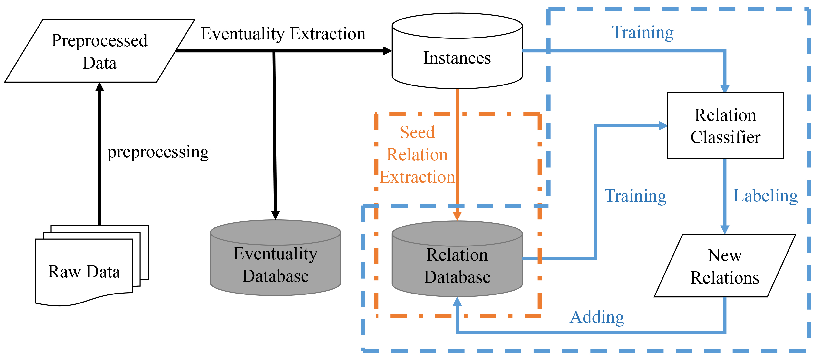
Figure 2. ASER extraction framework. The seed relation selection and the bootstrapping process are shown in the orange dash-dotted and blue dashed box respectively. Two gray databases are the resulted ASER.

3.1. System Overview

We first introduce the overall framework of our knowledge extraction system. The framework is shown in Figure 2. After textual data collection, we first preprocess the texts with the dependency parser. Then we perform eventuality extracting using pattern matching. For each sentence, if we find more than two eventualities, we first group these eventualities into pairs. For each pair, we generate one training instance, where each training instance contains two eventualities and their original sentence. After that, we extract seed relations from these training instances based on the less ambiguous connectives obtained from PDTB (Prasad et al., 2007). Finally, a bootstrapping process is conducted to learn more relations and train the new classifier repeatedly. In the following sub-sections, we will introduce each part of the system separately.

3.2. Corpora

To make sure the broad coverage of ASER, we select corpora from different resources (reviews, news, forums, social media, movie subtitles, e-books) as the raw data. The details of these datasets are as follows.

$\bullet$ Yelp: Yelp is a social media platform where users can write reviews for businesses, e.g., restaurants, hotels. The latest release of the Yelp dataset contains over five million reviews.

$\bullet$ New York Times (NYT): The NYT (Sandhaus and Evan, 2008) corpus contains over 1.8 million news articles from the NYT throughout 20 years (1987 - 2007).

Table 4. Statistics of used corpora. (M means millions.)

Name	# Sentences	# Tokens	# Instances	# Eventualities
Yelp	48.9M	758.3M	54.2M	20.5M
NYT	56.8M	1,196.9M	41.6M	23.9M
Wiki	105.1M	2,347.3M	38.9M	38.4M
Reddit	235.9M	3,373.2M	185.7M	82.6M
Subtitles	445.0M	3,164.1M	137.6M	27.0M
E-books	27.6M	618.6M	22.1M	11.1M
Overall	919.2M	11,458.4M	480.1M	194.0M

$\bullet$ Wiki: Wikipedia is one of the largest free knowledge dataset. To build ASER, we select the English version of Wikipedia.

$\bullet$ Reddit: Reddit is one of the largest online forums. In this work, we select the anonymized post records over one period month.

$\bullet$ Movie Subtitles: The movie subtitles corpus was collected by (Lison and Tiedemann, 2016) and we select the English subset, which contains subtitles for more than 310K movies.

$\bullet$ E-books: The last resource we include is the free English electronic books from Project Gutenberg.

We merge these resources as a whole to perform knowledge extraction. The statistics of different corpora are shown in Table 4.

Algorithm 1 Eventuality Extraction with One Pattern $P_{i}$

INPUT: Parsed dependency graph $D$, center verb $v$. Positive dependency edges $P_{i}^{p}$, optional edges $P_{i}^{o}$, and negative edges $P_{i}^{n}$. OUTPUT: Extracted eventuality $E$.

1:Initialize eventuality $E$.

2:for Each connection $d$ (a relation and the associated word) in positive dependency edges $P_{i}^{p}$ do

3:    if Find $d$ in $D$ then

4:        Append $d$ in $E$.

5:    else

6:        Return NULL.

7:    end if

8:end for

9:for Each connection $d$ in optional dependency edges $P_{i}^{o}$ do

10:    if Find $d$ in $D$ then

11:        Append $d$ in $E$.

12:    end if

13:end for

14:for Each connection $d$ in negative dependency edges $P_{i}^{n}$ do

15:    if Find $d$ in $D$ then

16:        Return NULL.

17:    end if

18:end for

19:Return $E$

3.3. Preprocessing and Eventuality Extraction

For each sentence $s$, we first parse it with the Stanford Dependency Parser. We then filter out all the sentences that contain clauses. As each sentence may contain multiple eventualities and verbs are the centers of them, we first extract all verbs. To make sure that all the extracted eventualities are semantically complete without being too complicated, we design 14 patterns to extract the eventualities via pattern matching. Each of the patterns contains three kinds of dependency edges: positive dependency edges, optional dependency edges, and negative dependency edges. All positives edges are shown in Table 2. Six more dependency relations (advmod, amod, nummod, aux, compound, and neg) are optional dependency edges that can associate with any of the selected patterns. We omit all optional edges in the table because they are the same for all patterns. All other dependency edges are considered are negative dependency edges, which are designed to make sure all the extracted eventualities are semantically complete and all the patterns are exclusive with each other. Take sentence ‘I have a book’ as an example, we will only select $<$‘I’, ‘have’, ‘book’$>$ rather than $<$‘I’, ‘have’$>$ as the valid eventuality, because ‘have’-dobj-‘book’ is a negative dependency edge for pattern ‘s-v’. For each verb $v$ and each pattern, we first put it in the position of $v_{1}$ and then try to find all the positive dependency edges. If we can find all the positive dependency edges around the center verb we consider it as one potential valid eventuality and then add all the words connected via those optional dependency edges. In the end, we will check if any negative dependency edge can be found in the dependency graph. If not, we will keep it as one valid eventuality. Otherwise, we will disqualify it. The pseudo-code of our extraction algorithm is shown in Algorithm 1. The time complexity of eventuality extraction is $\mathcal{O}(|S|\cdot|D|\cdot|v|)$ where $|S|$ is the number of sentences, $|D|$ is the average number of dependency edges in a dependency parse tree, and $|v|$ is the average number of verbs in a sentence.

Table 5. Selected seed connectives. Here relations are directed relation from $E_{1}$ to $E_{2}$. Each relation can have multiple seed connectives, where the corresponding connectives are highlighted as boldface.

Relation Type	Seed Patterns
Precedence	$E_{1}$ before $E_{2}$; $E_{1}$ , then $E_{2}$; $E_{1}$ till $E_{2}$; $E_{1}$ until $E_{2}$
Succession	$E_{1}$ after $E_{2}$; $E_{1}$ once $E_{2}$
Synchronous	$E_{1}$, meanwhile $E_{2}$; $E_{1}$ meantime $E_{2}$; $E_{1}$, at the same time $E_{2}$
Reason	$E_{1}$, because $E_{2}$
Result	$E_{1}$, so $E_{2}$; $E_{1}$, thus $E_{2}$; $E_{1}$, therefore $E_{2}$; $E_{1}$, so that $E_{2}$
Condition	$E_{1}$, if $E_{2}$; $E_{1}$, as long as $E_{2}$
Contrast	$E_{1}$, but $E_{2}$; $E_{1}$, however $E_{2}$; $E_{1}$, , by contrast $E_{2}$; $E_{1}$, , in contrast $E_{2}$; $E_{1}$, , on the other hand, $E_{2}$; $E_{1}$, , on the contrary, $E_{2}$
Concession	$E_{1}$, although $E_{2}$
Conjunction	$E_{1}$ and $E_{2}$; $E_{1}$, also $E_{2}$;
Instantiation	$E_{1}$, for example $E_{2}$; $E_{1}$, for instance $E_{2}$
Restatement	$E_{1}$, in other words $E_{2}$
Alternative	$E_{1}$ or $E_{2}$; $E_{1}$, unless $E_{2}$; $E_{1}$, as an alternative $E_{2}$; $E_{1}$, otherwise $E_{2}$
ChosenAlternative	$E_{1}$, $E_{2}$ instead
Exception	$E_{1}$, except $E_{2}$

3.4. Eventuality Relation Extraction

For each training instance, we use a two-step approach to decide the relations between the two eventualities.

We first extract seed relations from the corpora by using the unambiguous connectives obtained from PDTB (Prasad et al., 2007). According to PDTB’s annotation manual, we found that some of the connectives are more unambiguous than the others. For example, in the PDTB annotations, the connective ‘so that’ is annotated 31 times and is only with the Result relation. On the other hand, the connective ‘while’ is annotated as Conjunction 39 times, Contrast 111 times, expectation 79 times, and Concession 85 times. When we identify connectives like ‘while’, we can not determine the relation between the two eventualities related to it. Thus, we choose connectives that are less ambiguous, where more than 90% annotations of each are indicating the same relation, to extract seed relations. The selected connectives are listed in Table 5. Formally, we denote one informative connective word(s) and its corresponding relation type as $c$ and $T$. Given a training instance $x$=($E_{1}$, $E_{2}$, $s$), if we can find a connective $c$ such that $E_{1}$ and $E_{2}$ are connected by $c$ according to the dependency parse, we will select this instance as an instance for relation type $T$.

Since the seed relations extracted with selected connectives can only cover the limited number of the knowledge, we use a bootstrapping framework to incrementally extract more eventuality relations. Bootstrapping (Agichtein and Gravano, 2000) is a commonly used technique in information extraction. Here we use a neural network based approach to bootstrap. The general steps of bootstrapping are as follows.

$\bullet$ Step 1: Use the extracted seed training instances as the initial labeled training instances.

$\bullet$ Step 2: Train a classifier based on labeled training instances.

$\bullet$ Step 3: Use the classifier to predict relations of each training instance. If the prediction confidence of certain relation type $T$ is higher than the selected threshold, we will label this instance with $T$ and add it to the labeled training instances. Then go to Step 2.

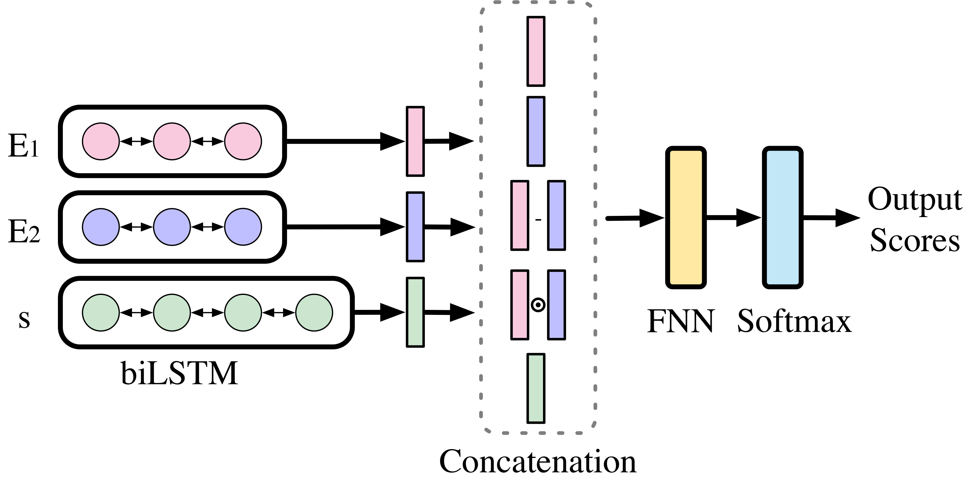
Figure 3. The overview of the neural classifier. For each instance $x=(E_{1},E_{2},s)$, we first encode the information of two eventualities $E_{1}$, $E_{2}$ and the original sentence $s$ with three bidirectional LSTMs (Hochreiter and Schmidhuber, 1997) module and the output representations are $h_{E_{1}}$, $h_{E_{2}}$ and $h_{s}$ respectively. We then concatenate $h_{E_{1}}$, $h_{E_{2}}$, $h_{E_{1}}-h_{E_{2}}$, $h_{E_{1}}\circ h_{E_{2}}$ and $h_{s}$ together, where $\circ$ indicates the element-wise multiplication, and feed them to a two-layer feed forward network. In the end, we use a softmax function to generate scores for different relation types.

The neural classifier architecture is shown in Figure 3. In the training process, we randomly select labelled training instances as positive examples and unlabelled training instances as negative examples. The cross-entropy is used as the loss and the whole model is updated via Adam (Kingma and Ba, 2015). In the labeling process, for each training instance $x$, the classifier can predict a score for each relation type. For any relation type, if the output score is larger than a threshold $\tau_{k}$, where $k$ is the number of bootstrapping iteration, we will label $x$ with that relation type. To avoid error accumulation, we also use the annealing strategy to increase the threshold $\tau_{k}=\tau_{0}+(1-\tau_{0})/(1+\exp{(-(k-K/2))})$, where $K$ is the total iteration number. The complexities of both training and labeling processes in $k^{th}$ iteration are linear to the number of parameters in LSTM cell $|L|$, the number of training examples $|I_{{train}_{k}}|$, and the number of instances to predict $|I_{{predict}_{k}}|$ in $k^{th}$ iteration. So the overall complexity in $k^{th}$ iteration is $\mathcal{O}(|L|\cdot(|I_{{train}_{k}}|+|I_{{predict}_{k}}|))$.

Used hyper-parameters and other implementation details are as follows: For preprocessing, we first parse all raw corpora with the Stanford Dependency parser, which costs eight days with two 12-core Intel Xeon Gold 5118 CPUs. After that, We extract eventualities, build the training instance set, and extract seed relations, which costs two days with the same CPUs. For bootstrapping, Adam optimizer (Kingma and Ba, 2015) is used and the initial learning rate is 0.001. The batch size is 512. We use GloVe (Pennington et al., 2014) as the pre-trained word embeddings. The dropout rate is 0.2 to prevent overfitting. The hidden sizes of LSTMs are 256 and the hidden size of the two-layer feed forward network with ReLU is 512. As relation types belonging to different categories could both exist in one training instance, in each bootstrapping iteration, four different classifiers are trained corresponding to four categories (Temporal, Contingency, Comparison, Temporal). Each classifier predicts the types belong to that category or ‘None’ of each instance. Therefore, classifiers do not influence each other so that they can be processed in parallel. Each iteration using ASER (core) takes around one hour with the same CPUs and four TITAN X GPUs. We spend around eight hours predicting ASER (full) with the learned classifier in the 10th iteration.

4. Inference over ASER

In this section, we provide two kinds of inferences (eventuality retrieval and relation retrieval) based on ASER. For each of them, inferences over both one-hop and multi-hops are provided. Complexities of these two retrieval algorithms are both $\mathcal{O}(A^{k})$, where $A$ is the number of average adjacent eventualities per eventuality and $k$ is the number of hops. In this section, we show how to conduct these inferences over one-hop and two-hop as the demonstration.

4.1. Eventuality Retrieval

The eventuality retrieval inference is defined as follows. Given a head eventuality $E_{h}$ and a relation list ${\mathcal{L}}$ = ($R_{1},R_{2},...,R_{k}$), find related eventualities and their associated probabilities such that for each eventuality $E_{t}$ we can find a path, which contains all the relations in ${\mathcal{L}}$ in order from $E_{h}$ to $E_{t}$.

4.1.1. One-hop Inference

For the one-hop inference, we assume the target relation is $R_{1}$. We then define the probability of any potential tail eventuality $E_{t}$ as:

(1) $$P(E_{t}|E_{h},R_{1})=\frac{f(E_{h},R_{1},E_{t})}{\sum_{E_{t}^{\prime},s.t.,(E_{t},R_{1})\in ASER}f(E_{h},R_{1},E_{t}^{\prime})},$$

where $f(E_{h},R_{1},E_{t})$ is the relation weight, which is defined in Definition 3. If no eventuality is connected with $E_{h}$ via $R_{1}$, $P(E^{\prime}|E_{h},R)$ will be 0 for any $E^{\prime}\in{\mathcal{E}}$.

4.1.2. Two-hop Inference

On top of Eq. (1), it is easy for us to define the probability of $E_{t}$ on two-hop setting. Assume the two relations are $R_{1}$ and $R_{2}$ in order. We can define the probability as follows:

(2) $$P(E_{t}|E_{h},R_{1},R_{2})=\sum_{E_{m}\in{\mathcal{E}}_{m}}P(E_{m}|E_{h},R_{1})P(E_{t}|E_{m},R_{2}),$$

where ${\mathcal{E}}_{m}$ is the set of intermediate eventuality $E_{m}$ such that $(E_{h},R_{1},E_{m})$ and $(E_{m},R_{2},E_{t})\in ASER$.

4.2. Relation Retrieval

The relation retrieval inference is defined as follows. Given two eventualities $E_{h}$ and $E_{t}$, find all relation lists and their probabilities such that for each relation list ${\mathcal{L}}$ = ($R_{1},R_{2},...,R_{k}$), we can find a path from $E_{h}$ to $E_{t}$, which contains all the relations in ${\mathcal{L}}$ in order.

4.2.1. One-hop Inference

Assuming that the path length is one, we define the probability of one relation $R$ exist from $E_{h}$ to $E_{t}$ as:

(3) $$P(R|E_{h},E_{t})=\frac{f(E_{h},R,E_{t})}{\sum_{R^{\prime}\in{\mathcal{R}}}f(E_{h},R^{\prime},E_{t})},$$

where ${\mathcal{R}}$ is the relation set.

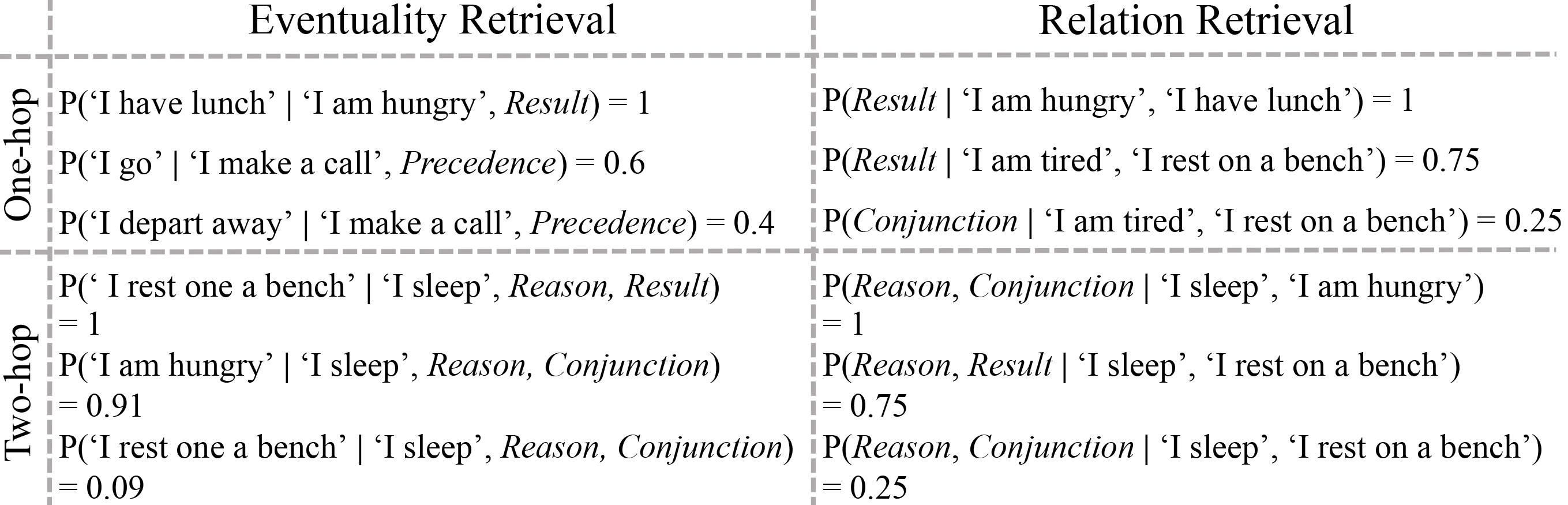
Figure 4. Examples of inference over ASER.

4.2.2. Two-hop Inference

Similarly, given two eventualities $E_{h}$ and $E_{t}$, we define the probability of a two-hop connection ($R_{1}$, $R_{2}$) between them as follows:

$$P(R_{1},R_{2}|E_{h},E_{t}) =\sum_{E_{m}\in{\mathcal{E}}_{m}}P(R_{1},R_{2},E_{m}|E_{h},E_{t})$$

(4) $$=\sum_{E_{m}\in{\mathcal{E}}_{m}}P(R_{1}|E_{h})P(E_{m}|R_{1},E_{h})P(R_{2}|E_{m},E_{t}),$$

where $P(R|E_{h})$ is the probability of relation $R$, given head eventuality $E_{h}$, and is defined as follows:

(5) $$P(R|E_{h})=\frac{\sum_{E_{t},s.t.,(E_{t},R)\in ASER}f(E_{h},R,E_{t})}{\sum_{R^{\prime}\in{\mathcal{R}}}\sum_{E_{t},s.t.,(E_{t},R)\in ASER}f(E_{h},R^{\prime},E_{t})}.$$

4.3. Case Study

Table 6. Statistics and annotations of the eventuality extraction. # Eventuality and # Unique means the total number and the unique number of extracted eventualities using corresponding patterns (‘M’ stands for millions). # Agreed means the number of agreed eventualities among five annotators. # Valid means the number valid eventualities labeled by annotators. Accuracy (Acc.)=# Valid/# Agrees. The Overall accuracy is calculated based on the pattern distribution.

Pattern	# Eventuality	# Unique	# Agreed	# Valid	Acc.
s-v	109.0M	22.1M	171	158	92.4%
s-v-o	129.0M	60.0M	181	173	95.6%
s-v-a	5.2M	2.1M	195	192	98.5%
s-v-o-o	3.5M	1.7M	194	187	96.4%
s-be-a	89.9M	29.0M	189	188	99.5%
s-v-be-a	1.2M	0.5M	190	187	98.4%
s-v-be-o	1.2M	0.7M	186	171	91.9%
s-v-v-o	12.4M	6.6M	193	185	95.9%
s-v-v	8.7M	2.7M	185	155	83.8%
s-be-a-p-o	13.2M	8.7M	189	185	97.9%
s-v-p-o	39.0M	23.5M	178	161	90.4%
s-v-o-p-o	27.2M	19.7M	181	167	92.2%
spass-v	15.1M	6.2M	177	155	87.6%
spass-v-p-o	13.5M	10.3M	188	177	94.1%
Overall	468.1M	194.0M	—	—	94.5%

In this section, we showcase several interesting inference examples with ASER in Figure 4, which is conducted over the extracted sub-graph of ASER shown in Figure 1. By doing inference over eventuality retrieval, we can easily find out that ‘I am hungry’ usually results in having lunch and the eventuality ‘I make a call’ often happens before someone goes or departs. More interestingly, leveraging the two-hop inference, given the eventuality ‘I sleep’, we can find out an eventuality ‘I rest on a bench’ such that both of them are caused by the same reason, which is ‘I am tired’ in this example. On the other hand, we can also retrieve possible relations between eventualities. For example, we can know that ‘I am hungry’ is most likely the reason for ‘I have lunch’ rather than the other way around. Similarly, over the 2-hop inference, we can find out that even though ‘I am hungry’ has no direct relation with ‘I sleep’, ‘I am hungry’ often appears at the same time with ‘I am tired’, which is one plausible reason for ‘I sleep’.

5. Intrinsic Evaluation

In this section, we present intrinsic evaluation to assess the quantity and quality of extracted eventualities.

5.1. Eventualities Extraction

We first present the statistics of the extracted eventualities in Table 6, which shows that simpler patterns like ‘s-v-o’ appear more frequently than the complicated patterns like ‘s-v-be-a’.

The distribution of extracted eventualities is shown in Figure 5. In general, the distribution of eventualities follows the Zipf’s law, where only a few eventualities appear many times while the majority of eventualities appear only a few times. To better illustrate the distribution of eventualities, we also show several representative eventualities along with their frequencies and we have two observations. First, eventualities which can be used in general cases, like ‘You think’, appear much more times than other eventualities. Second, eventualities contained in ASER are more related to our daily life like ‘Food is tasty’ or ‘I sleep’ rather than domain-specific ones such as ‘I learn python’.

After extracting the eventualities, we employ the Amazon Mechanical Turk platform (MTurk) for annotations. For each eventuality pattern, we randomly select 200 extracted eventualities and then provide these extracted eventualities along with their original sentences to the annotators. In the annotation task, we ask them to label whether one auto-extracted eventuality phrase can fully and precisely represent the semantic meaning of the original sentence. If so, they should label them with ‘Valid’. Otherwise, they should label it with ‘Not Valid’. For each eventuality, we invite four workers to label and if at least three of them give the same annotation result, we consider it to be one agreed annotation. Otherwise, this extraction is considered as disagreed. In total, we spent $201.6. The detailed result is shown in Table 6. We got 2,597 agreed annotations out of 2,800 randomly selected eventualities, and the overall agreement rate is 92.8%, which indicates that annotators can easily understand our task and provide consistent annotations. Besides that, as the overall accuracy is 94.5%, the result proves the effectiveness of the proposed eventuality extraction method.

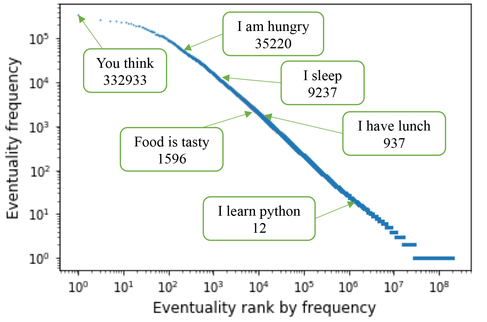
Figure 5. Distribution of eventualities by their frequencies.

5.2. Relations Extraction

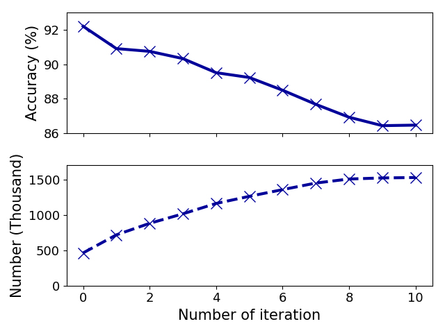
(a) Statistics and evaluation of bootstrapping.

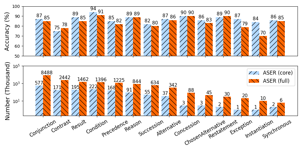
(b) Distribution and accuracy of different relation types.

Figure 6. Human Evaluation of the bootstrapping process. Relation Co_Occurrence is not included in the figures since it is not influenced by the bootstrapping.

In this section, we evaluate the quantity and quality of extracted relations in ASER. Here, to make sure the quality of the learned bootstrapping model, we filter out eventuality and eventuality pairs that appear once and use the resulting training instances to train the bootstrapping model. The KG extracted from the selected data is called the core part of ASER. Besides that, after the bootstrapping, we directly apply the final bootstrapping model on all training instances and get the full ASER. In this section, we will first evaluate the bootstrapping process and then evaluate relations in two versions of ASER (core and full).

For the bootstrapping process, similar to the evaluation of eventuality extraction, we invite annotators from Amazon Turk to annotate the extracted edges. For each iteration, we randomly select 100 edges for each relation type. For each edge, we generate a question by asking the annotators if they think certain relation exists between the two eventualities. If so, they should label it as ‘Valid’. Otherwise, they should label it as ‘Not Valid’. Similarly, if at least three of the four annotators give the same annotation result, we consider it to be an agreed one and the overall agreement rate is 82.8 %. For simplicity, we report the average accuracy, which is calculated based on the distribution of different relation types, as well as the total number of edges in Figure 6(a). The number of edges grows fast at the beginning and slows down later. After ten iterations of bootstrapping, the number of edges grows four times with the decrease of less than 6% accuracy (from 92.3% to 86.5%).

Finally, we evaluate the core and full versions of ASER. For both versions of ASER, we randomly select 100 edges per relation type and invite annotators to annotate them using the same way as we annotating the bootstrapping process. Together with the evaluation on bootstrapping, we spent $1698.4. The accuracy along with the distribution of different relation types are shown in Figure 6(b). We also compute the overall accuracy for the core and full versions of ASER by computing the weighted average of these accuracy scores based on the frequency. The overall accuracies of the core and full versions are 86.5% and 84.3% respectively, which is comparable with KnowlyWood (Tandon et al., 2015) (85%), even though Knowlywood only relies on human designed patterns and ASER involves bootstrapping. From the result, we observe that, in general, the core version of ASER has a better accuracy than the full version, which fits our understanding that the quality of those rare eventualities might not be good. But from another perspective, the full version of ASER can cover much more relations than the core version with acceptable accuracy.

5.3. Comparison with ConceptNet

We study the relationship between ASER and the commonsense knowledge in ConceptNet (Liu and Singh, 2004), or previously called Open Mind Common Sense (OMCS) (Singh et al., 2002). The original ConceptNet contains 600K commonsense triplets and 75K among them involve eventualities, such as (sleep, HasSubevent, dream) and (wind, CapableOf, blow to east). All relations in ConceptNet are human-defined. We select all four commonsense relations (HasPrerequisite, Causes, MotivatedByGoal, and HasSubevent) that involve eventualities to examine how many relations are covered in ASER. Here by covered, we mean that for a given ConceptNet pair $(E_{o1},E_{o2})$, we can find an edge $x=(E_{a1},E_{a2},c)$ in ASER such that $E_{o1}$ = $E_{a1}$, $E_{o1}$ = $E_{a1}$. The detailed statistic of coverages are shown in Table 7.

Table 7. Statistics of selected OMCS data. we only select ConceptNet pairs that involve eventualities.

Relation	# Examples	# Covered	Coverage
HasPrerequisite	22,389	21,515	96.10%
Causes	14,065	12,605	89.62%
MotivatedByGoal	11,911	10,692	89.77%
HasSubevent	30,074	28,856	95.95%
Overall	78,439	73,668	93.92%

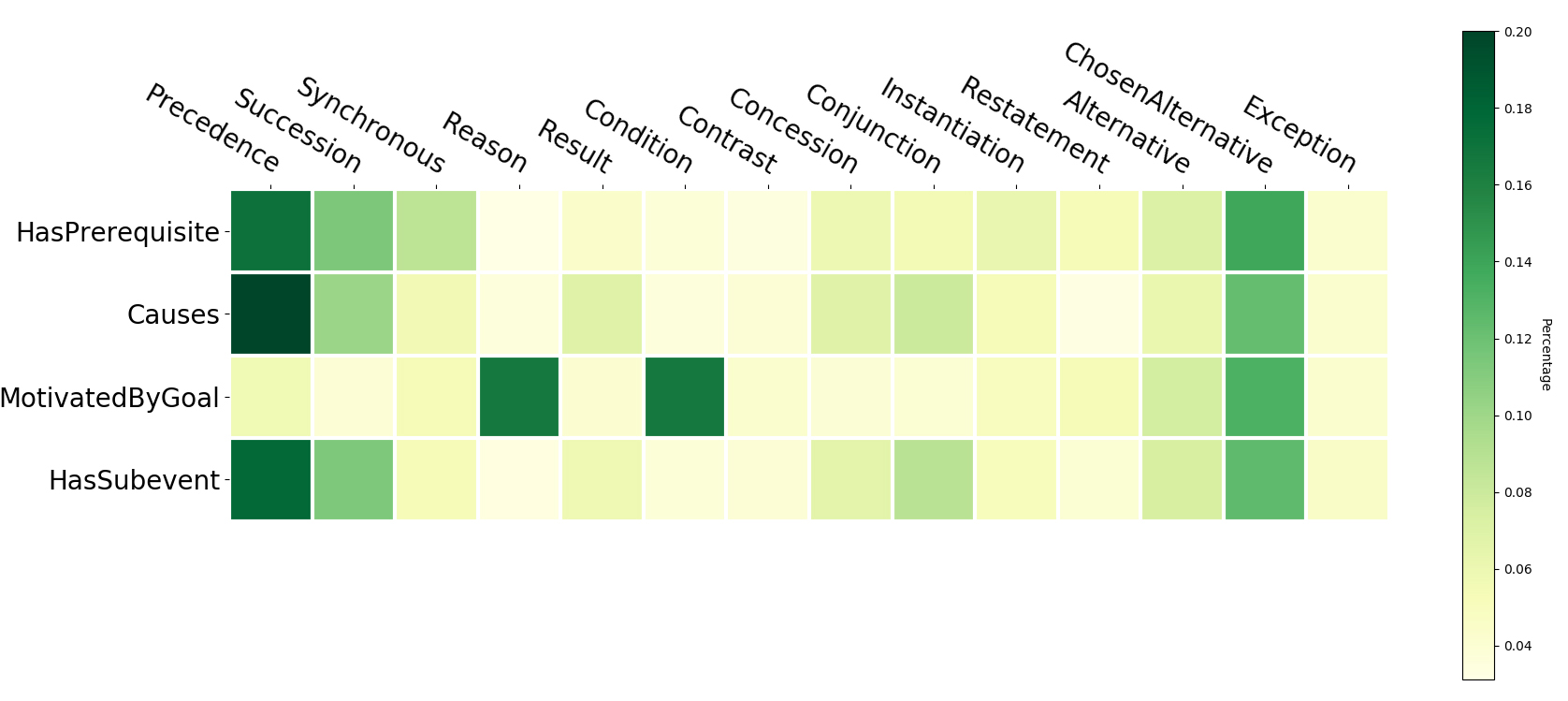
Figure 7. Heatmap of overlapping between OMCS and ASER relations. For each OMCS relation, the distribution of matched ASER edges is computed. Darker color indicates more overlaps.

Moreover, to show the connection between the ConceptNet and ASER, we use a heat map to show the distribution of their relation pairs . The result is shown in Figure 7, where darker color indicates more coverage, and we observe many interesting findings. First, we can find a strong connection between Causes and Precedence, which fits our understanding that eventualities happen first is probably the reason for the eventualities happen later. For example, I eat and then I am full, where ‘we eat’ is the reason of ‘I am full’. Such correlation between temporal and causal relations is also observed in (Ning et al., 2018). Second, most of the MotivatedByGoal pairs appear in the Reason or Condition relation in ASER, which makes sense because the motivation can be both the reason or the condition. For example, ‘I am hungry’ can be viewed as both the motivation and the requirement of ‘I eat’ and both ‘I eat because I am hungry’ and ‘I eat if I am hungry’ are valid statements. These observations demonstrate that the knowledge contained in ConceptNet can be effectively covered by ASER. Considering that ConceptNet is often criticized for its scale and ASER is two magnitude larger than ConceptNet, even though ASER may not be as accurate as ConceptNet, it could be a good supplement.

6. Extrinsic Evaluations

In this section, we select the Winograd Schema Challenge (WSC) task to evaluate whether the knowledge in ASER can help understand human language. Winograd Schema Challenge is known as related to commonsense knowledge and argued as a replacement of the Turing test (Levesque et al., 2011). Given two sentences $s_{1}$ and $s_{2}$, both of them contain two candidate noun phrases $n_{1}$ and $n_{2}$, and one targeting pronoun $p$. The goal is to detect the correct noun phrase $p$ refers to. Here is an example (Levesque et al., 2011).

(1) The fish ate the worm. It was hungry. Which was hungry?

Answer: the fish.

(2) The fish ate the worm. It was tasty. Which was tasty?

Answer: the worm.

This task is challenging because $s_{1}$ and $s_{2}$ are quite similar to each other (only one-word difference), but the result is totally reversed. Besides that, all the widely used features such as gender/number are removed, and thus all the conventional rule-based resolution system failed on this task. For example, in the above example, both fish and worm can be hungry or tasty by themselves. In this experiment, we select all 273 questions.

6.1. ASER for Winograd Schema Challenge

To demonstrate the effectiveness of ASER, we propose two methods of leveraging the knowledge in ASER to solve the WSC questions: (1) string match and inference over ASER; (2) Fine-tune pre-trained language models with knowledge in ASER.

6.1.1. String Match and Inference

For each question sentence $s$, we first extract eventualities with the same method introduced in Section 3.3 and then select eventualities $E_{n_{1}}$, $E_{n_{2}}$, and $E_{p}$ that contain candidates nouns $n_{1}$/$n_{2}$ and the target pronoun $p$ respectively. We then replace $n_{1}$, $n_{2}$, and $p$ with placeholder $X$, $Y$, and $P$, and hence generate the pseudo-eventualities $E_{n_{1}}^{\prime}$, $E_{n_{2}}^{\prime}$, and $E_{p}^{\prime}$. After that, if we can find the seed connectives in Table 5 between any two eventualities, we use the corresponding relation type as relation type $T$. Otherwise, we use Co_Occurrence as the relation type. To evaluate the candidate, we first replace the placeholder $P$ in $E_{p}^{\prime}$ with the corresponding placeholders $X$ or $Y$ and then use the following equation to define its overall plausibility score:

(6) $$F(n,p)=ASER_{R}(E_{n}^{\prime},E_{p}^{\prime}),$$

where $ASER_{R}(E_{n},E_{p})$ indicates the number of edges in ASER that can support that there exist one typed $T$ relation between the eventuality pairs $E_{n}^{\prime}$ and $E_{p}^{\prime}$. For each edge ($E_{h}$, $T$, $E_{t}$) in ASER, if it can fit the following three requirements:

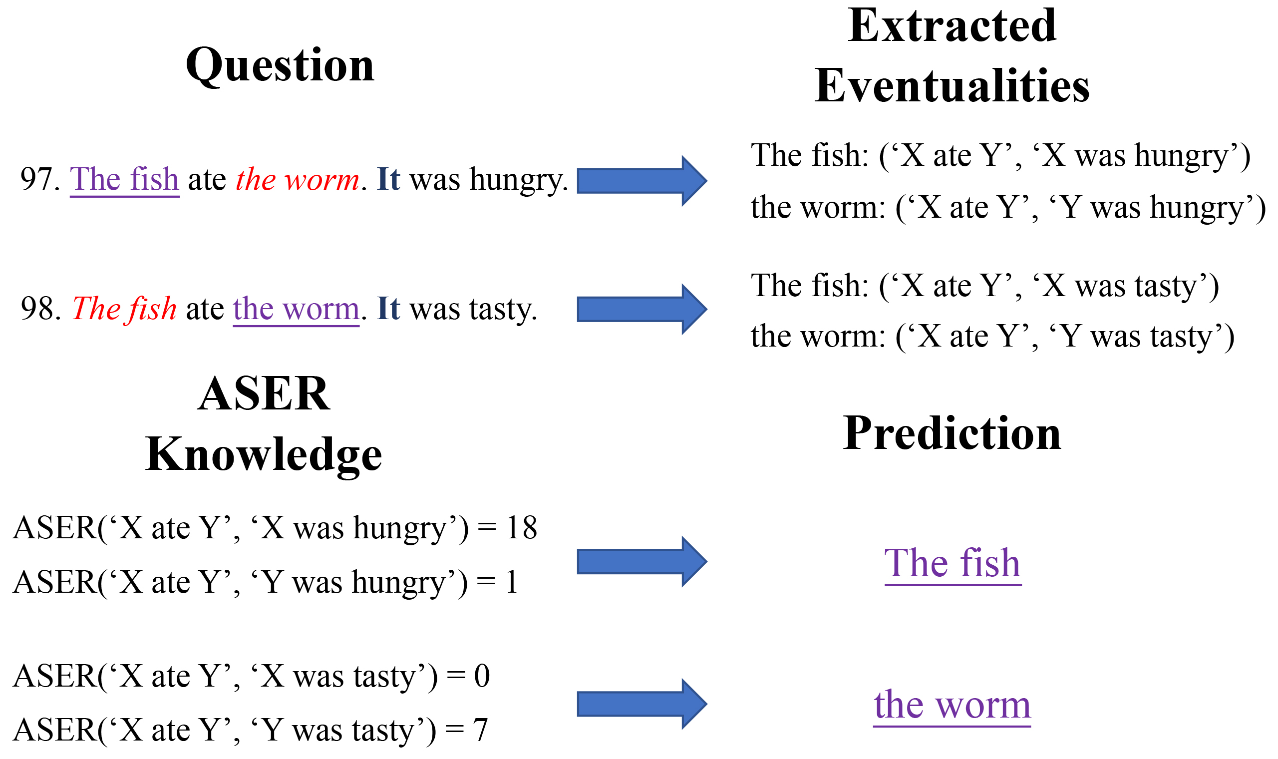
Figure 8. Example of using ASER to solve Winograd questions. The number before questions are the original question ID. Correct answer and the other candidate are labeled with purple underline and red italic font respectively.

1. $E_{h}$ = $E_{n}^{\prime}$ other than the words in the place holder positions.

2. $E_{t}$ = $E_{p}^{\prime}$ other than the words in the place holder positions.

3. Assume the word in the placeholder positions of $E_{h}$ and $E_{t}$ are $w_{h}$ and $w_{t}$ respectively, $w_{h}$ has to be same as $w_{t}$.

we consider that edge as a valid edge to support the observed eventuality pair. If any of $E_{n}$ and $E_{p}$ cannot be extracted with our patterns, we will assign 0 to $F(n,p)$. We then predict the candidate with the higher score to be the correct reference. If both of them have the same score (including 0), we will make no prediction. At the current stage, We only use one-hop relations in ASER to perform the inference. One example of using inference over ASER to solve WSC questions is shown in Figure 8, our model can correctly resolve ‘it’ to ‘fish’ in question 97, because 18 edges in ASER support that the subject of ‘eat’ should be ‘hungry’, while only one edge supports the object of ‘eat’ should be ‘hungry’. Similarly, our model can correctly resolve ‘it’ to ‘the worm’ in question 98, because seven edges in ASER support that the object of ‘eat’ should be ‘tasty’ while no edge supports that the subject of ‘eat’ should be ‘tasty’.

6.1.2. Fine-Tune Language Model

Recently, Pre-trained Language models (e.g., BERT (Devlin et al., 2019) and GPT-2 (Radford et al., 2019)) have demonstrated the strong ability to represent knowledge with deep models and have been proved to be very helpful for natural language understanding tasks like WSC. To evaluate if the knowledge in ASER can further help these language models, we propose to jointly leverage ASER and the language models to solve the WSC questions.

For each question sentence $s$, we first extract eventualities that contain the target pronoun $E_{p}$ and two candidates $E_{c}$ and then select all edges ($E_{1}$, $R$, $E_{2}$) from ASER such that $E_{1}$ and $E_{2}$ contains the verb of $E_{p}$ and $E_{c}$ respectively and there exists one common word in $E_{1}$ and $E_{2}$. After that, for each selected edge, we then replace the common word in $E_{2}$ with a pronoun, which we assume refers to the same word in $E_{1}$, and thus create a pronoun coreference example in the WSC style. For example, given the edge (‘boy eats food’, Reason, ‘boy is hungry’), we create an example ‘boy eats food because he is hungry’ and we know that ‘he’ refers to ‘boy’. Then, we fine-tune the pre-trained language models (BERT-large in our experiments) using these automatically generated data in the same way as (Kocijan et al., 2019). We denote this model as BERT+ASER. In the original paper (Kocijan et al., 2019), they also tried using another dataset WSCR (Rahman and Ng, 2012) to fine-tune the language model, which is shown to be very helpful. Thus we also consider using both WSCR and ASER to fine-tune language models, which is denoted as BERT+ASER+WSCR.

6.2. Baseline Methods.

We first compare ASER with Conventional WSC solutions:

• Knowledge Hunting (Emami et al., 2018) first search commonsense knowledge on search engines (e.g., Google) for the Winograd questions and then leverages rule-based methods to make the final predictions based on the collected knowledge.

• LM model (Trinh and Le, 2018) is the language model trained with very large-scale corpus and tuned specifically for the WSC task. We denote the best single language model and the ensemble model as LM (single) and LM (ensemble) respectively.

Besides that, we also compare with the selectional preference (SP) based method (Zhang et al., 2019). Following the original setting, two resources (human annotation and Posterior Probability) of SP knowledge are considered and we denote them as SP (human) and SP (PP) respectively. Last but not least, we also compare with following pre-trained language models:

• GPT-2: GPT-2 (Radford et al., 2019) is the current best unsupervised model for the WSC task. We report the performance of its best model (1542 million parameters).

• BERT: As shown in (Kocijan et al., 2019), we can first convert the original WSC task into a token prediction task and then BERT (Devlin et al., 2019) can be used to predict the results. As shown in the paper, the large model of BERT outperforms the base model significantly and we only report the performance of the large model. We denote the BERT model without or with fine-tuning on WSCR as BERT and BERT+WSCR respectively.

The official released codes/models of all baseline methods are used to conduct the experiments.

Table 8. Experimental results on Winograd Schema Challenge. $\surd$ indicates the number of correct answers, $\times$ indicates the number of wrong answers, and $NA$ means that the model cannot give a prediction. $A_{p}$ means the prediction accuracy without $NA$ examples, and $A_{o}$ means the overall accuracy.

Methods	$\surd$	$\times$	NA	$A_{p}$	$A_{o}$
Random Guess	137	136	0	50.2%	50.2%
Knowledge Hunting (Emami et al., 2018)	119	79	75	60.1%	57.3%
LM (single) (Trinh and Le, 2018)	149	124	0	54.5%	54.5%
LM (Ensemble) (Trinh and Le, 2018)	168	105	0	61.5%	61.5%
SP (human) (Zhang et al., 2019)	15	0	258	100%	52.7%
SP (PP) (Zhang et al., 2019)	50	26	197	65.8%	54.4%
GPT-2 (Radford et al., 2019)	193	80	0	70.7%	70.7%
BERT (Kocijan et al., 2019)	169	104	0	61.9%	61.9%
BERT+WSCR (Kocijan et al., 2019)	195	78	0	71.4%	71.4%
ASER (inference)	63	27	183	70.0%	56.6%
BERT+ASER	177	96	0	64.5%	64.5%
BERT+WSCR+ASER	198	75	0	72.5%	72.5%

6.3. Result Analysis.

From the result in Table 8, we can make the following observations:

1. Pure knowledge-based methods (Knowledge Hunting and ASER (inference)) can be helpful, but their help is limited, which is mainly because of their low coverage and the lack of good application methods. For example, when we use ASER, we only consider the string match, which is obviously not good enough.

2. Pre-trained language models achieve much better performance, which is mainly due to their deep models and large corpora they are trained on. Besides that, as already shown in (Kocijan et al., 2019), fine-tuning on a similar dataset like WSCR can be very helpful.

3. Adding knowledge from ASER can help state-of-the-art models. In our experiments, as we do not change any model architectures or hyper-parameters, we surprisingly find out that adding some related ASER knowledge can be helpful, which further proves the value of ASER.

7. Conclusions

In this paper, we introduce ASER, a large-scale eventuality knowledge graph. We extract eventualities from texts based on the dependency graphs. Then we build seed relations among eventualities using unambiguous connectives found from PDTB and use a neural bootstrapping framework to extract more relations. ASER is the first large-scale eventuality KG using the above strategy. We conduct systematic experiments to evaluate the quality and applications of the extracted knowledge. Both human and extrinsic evaluations show that ASER is a promising large-scale eventuality knowledge graph with great potential in many downstream tasks.

References

- (1)
- Agichtein and Gravano (2000) Eugene Agichtein and Luis Gravano. 2000. Snowball: Extracting relations from large plain-text collections. In Proceedings of ACM DL 2000. 85–94.
- Aguilar et al. (2014) Jacqueline Aguilar, Charley Beller, Paul McNamee, Benjamin Van Durme, Stephanie Strassel, Zhiyi Song, and Joe Ellis. 2014. A comparison of the events and relations across ace, ere, tac-kbp, and framenet annotation standards. In Workshop on EVENTS: Definition, Detection, Coreference, and Representation. 45–53.
- Auer et al. (2007) Sören Auer, Christian Bizer, Georgi Kobilarov, Jens Lehmann, Richard Cyganiak, and Zachary G. Ives. 2007. DBpedia: A Nucleus for a Web of Open Data. In Proceedings of ISWC-ASWC 2007. 722–735.
- Bach (1986) Emmon Bach. 1986. The algebra of events. Linguistics and philosophy 9, 1 (1986), 5–16.
- Baker et al. (1998) Collin F. Baker, Charles J. Fillmore, and John B. Lowe. 1998. The Berkeley FrameNet Project. In Proceedings of COLING-ACL 1998. 86–90.
- Banko et al. (2007) Michele Banko, Michael J. Cafarella, Stephen Soderland, Matthew Broadhead, and Oren Etzioni. 2007. Open Information Extraction from the Web. In Proceedings of IJCAI 2007. 2670–2676.
- Berant et al. (2013) Jonathan Berant, Andrew Chou, Roy Frostig, and Percy Liang. 2013. Semantic Parsing on Freebase from Question-Answer Pairs. In Proceedings of EMNLP 2013. 1533–1544.
- Bollacker et al. (2008) Kurt D. Bollacker, Colin Evans, Praveen Paritosh, Tim Sturge, and Jamie Taylor. 2008. Freebase: a collaboratively created graph database for structuring human knowledge. In Proceedings of SIGMOD 2008. 1247–1250.
- Carlson et al. (2010) Andrew Carlson, Justin Betteridge, Bryan Kisiel, Burr Settles, Estevam R. Hruschka Jr., and Tom M. Mitchell. 2010. Toward an Architecture for Never-Ending Language Learning. In Proceedings of AAAI 2010. 1306–1313.
- Dalvi et al. (2018) Bhavana Dalvi, Lifu Huang, Niket Tandon, Wen-tau Yih, and Peter Clark. 2018. Tracking State Changes in Procedural Text: a Challenge Dataset and Models for Process Paragraph Comprehension. In Proceedings of NAACL-HLT 2018. 1595–1604.
- Devlin et al. (2019) Jacob Devlin, Ming-Wei Chang, Kenton Lee, and Kristina Toutanova. 2019. BERT: Pre-training of Deep Bidirectional Transformers for Language Understanding. In Proceedings of NAACL-HLT 2019. 4171–4186.
- Dong et al. (2014) Xin Dong, Evgeniy Gabrilovich, Geremy Heitz, Wilko Horn, Ni Lao, Kevin Murphy, Thomas Strohmann, Shaohua Sun, and Wei Zhang. 2014. Knowledge vault: A web-scale approach to probabilistic knowledge fusion. In Proceedings of KDD 2014. 601–610.
- Ehrlinger and Wöß (2016) Lisa Ehrlinger and Wolfram Wöß. 2016. Towards a Definition of Knowledge Graphs. In Proceedings of SEMANTiCS-SuCCESS 2016.
- Emami et al. (2018) Ali Emami, Noelia De La Cruz, Adam Trischler, Kaheer Suleman, and Jackie Chi Kit Cheung. 2018. A Knowledge Hunting Framework for Common Sense Reasoning. In Proceedings of EMNLP 2018. 1949–1958.
- Etzioni et al. (2004) Oren Etzioni, Michael Cafarella, and Doug Downey. 2004. WebScale Information Extraction in KnowItAll (Preliminary Results). In Proceedings of WWW 2004. 100–110.
- Fellbaum (1998) Christiane Fellbaum (Ed.). 1998. WordNet: an electronic lexical database. MIT Press.
- Hochreiter and Schmidhuber (1997) Sepp Hochreiter and Jürgen Schmidhuber. 1997. Long short-term memory. Neural computation 9, 8 (1997), 1735–1780.
- Jackendoff (1990) Ray Jackendoff (Ed.). 1990. Semantic Structures. Cambridge, Massachusetts: MIT Press.
- Kingma and Ba (2015) Diederick P Kingma and Jimmy Ba. 2015. Adam: A method for stochastic optimization. In Proceedings of ICLR 2015.
- Kocijan et al. (2019) Vid Kocijan, Ana-Maria Cretu, Oana-Maria Camburu, Yordan Yordanov, and Thomas Lukasiewicz. 2019. A Surprisingly Robust Trick for the Winograd Schema Challenge. In Proceedings of ACL 2019. 4837–4842.
- Lenat and Guha (1989) Douglas B. Lenat and R. V. Guha. 1989. Building Large Knowledge-Based Systems: Representation and Inference in the Cyc Project. Addison-Wesley.
- Levesque et al. (2011) Hector J Levesque, Ernest Davis, and Leora Morgenstern. 2011. The Winograd schema challenge.. In AAAI Spring Symposium: Logical formalizations of commonsense reasoning, Vol. 46. 47.
- Li et al. (2013) Qi Li, Heng Ji, and Liang Huang. 2013. Joint event extraction via structured prediction with global features. In Proceedings of ACL 2013. 73–82.
- Lison and Tiedemann (2016) Pierre Lison and Jörg Tiedemann. 2016. OpenSubtitles2016: Extracting Large Parallel Corpora from Movie and TV Subtitles. In Proceedings of LREC 2016.
- Liu and Singh (2004) Hugo Liu and Push Singh. 2004. ConceptNet–a practical commonsense reasoning tool-kit. BT technology journal 22, 4 (2004), 211–226.
- Meyers et al. (2004) Adam Meyers, Ruth Reeves, Catherine Macleod, Rachel Szekely, Veronika Zielinska, Brian Young, and Ralph Grishman. 2004. The NomBank Project: An Interim Report. In Proceedings of the Workshop Frontiers in Corpus Annotation@HLT-NAACL 2004.
- Ning et al. (2018) Qiang Ning, Zhili Feng, Hao Wu, and Dan Roth. 2018. Joint reasoning for temporal and causal relations. In ACL. 2278–2288.
- NIST (2005) NIST. 2005. The ACE evaluation plan.
- P. D. Mourelatos (1978) Alexander P. D. Mourelatos. 1978. Events, Processes, and States. Linguistics and Philosophy 2 (01 1978), 415–434.
- Palmer et al. (2005) Martha Palmer, Daniel Gildea, and Paul Kingsbury. 2005. The proposition bank: An annotated corpus of semantic roles. Computational linguistics 31, 1 (2005), 71–106.
- Pennington et al. (2014) Jeffrey Pennington, Richard Socher, and Christopher D. Manning. 2014. Glove: Global Vectors for Word Representation. In Proceedings of EMNLP 2014. 1532–1543.
- Prasad et al. (2007) Rashmi Prasad, Eleni Miltsakaki, Nikhil Dinesh, Alan Lee, Aravind Joshi, Livio Robaldo, and Bonnie L Webber. 2007. The penn discourse treebank 2.0 annotation manual. (2007).
- Pustejovsky et al. (2003) James Pustejovsky, Patrick Hanks, Roser Sauri, Andrew See, Robert Gaizauskas, Andrea Setzer, Dragomir Radev, Beth Sundheim, David Day, Lisa Ferro, et al. 2003. The timebank corpus. In Corpus linguistics, Vol. 2003. 40.
- Radford et al. (2019) Alec Radford, Jeff Wu, Rewon Child, David Luan, Dario Amodei, and Ilya Sutskever. 2019. Language Models are Unsupervised Multitask Learners. (2019).
- Rahman and Ng (2012) Altaf Rahman and Vincent Ng. 2012. Resolving Complex Cases of Definite Pronouns: The Winograd Schema Challenge. In Proceedings of EMNLP 2012. 777–789.
- Sandhaus and Evan (2008) Sandhaus and Evan. 2008. The New York Times Annotated Corpus LDC2008T19. (2008).
- Sap et al. (2019) Maarten Sap, Ronan LeBras, Emily Allaway, Chandra Bhagavatula, Nicholas Lourie, Hannah Rashkin, Brendan Roof, Noah A. Smith, and Yejin Choi. 2019. ATOMIC: An Atlas of Machine Commonsense for If-Then Reasoning. In Proceedings of AAAI 2019. 3027–3035.
- Singh et al. (2002) Push Singh, Thomas Lin, Erik T Mueller, Grace Lim, Travell Perkins, and Wan Li Zhu. 2002. Open Mind Common Sense: Knowledge acquisition from the general public. In Proceedings of OTM 2002. 1223–1237.
- Smith et al. (2018) Noah A. Smith, Yejin Choi, Maarten Sap, Hannah Rashkin, and Emily Allaway. 2018. Event2Mind: Commonsense Inference on Events, Intents, and Reactions. In Proceedings of ACL 2018. 463–473.
- Suchanek et al. (2007) Fabian M. Suchanek, Gjergji Kasneci, and Gerhard Weikum. 2007. Yago: a core of semantic knowledge. In Proceedings of WWW 2007. 697–706.
- Tandon et al. (2015) Niket Tandon, Gerard de Melo, Abir De, and Gerhard Weikum. 2015. Knowlywood: Mining Activity Knowledge From Hollywood Narratives. In Proceedings of CIKM 2015. 223–232.
- Trinh and Le (2018) Trieu H. Trinh and Quoc V. Le. 2018. A Simple Method for Commonsense Reasoning. CoRR abs/1806.02847 (2018).
- Wilks (1975) Yorick Wilks. 1975. A preferential, pattern-seeking, semantics for natural language inference. Artificial intelligence 6, 1 (1975), 53–74.
- Wu et al. (2012) Wentao Wu, Hongsong Li, Haixun Wang, and Kenny Q. Zhu. 2012. Probase: A Probabilistic Taxonomy for Text Understanding. In Proceedings of SIGMOD 2012. 481–492.
- Xue et al. (2015) Nianwen Xue, Hwee Tou Ng, Sameer Pradhan, Rashmi Prasad, Christopher Bryant, and Attapol Rutherford. 2015. The conll-2015 shared task on shallow discourse parsing. In CoNLL Shared Task. 1–16.
- Zhang et al. (2019) Hongming Zhang, Hantian Ding, and Yangqiu Song. 2019. SP-10K: A large-scale evaluation set for selectional preference acquisition. In Proceedings of ACL 2019. 722–731.