Dynamics of the critical Casimir force for a conserved order parameter
after a critical quench

Abstract

Fluctuation-induced forces occur generically when long-ranged correlations (e.g., in fluids) are confined by external bodies. In classical systems, such correlations require specific conditions, e.g., a medium close to a critical point. On the other hand, long-ranged correlations appear more commonly in certain non-equilibrium systems with conservation laws. Consequently, a variety of non-equilibrium fluctuation phenomena, including fluctuation-induced forces, have been discovered and explored recently. Here, we address a long-standing problem of non-equilibrium critical Casimir forces emerging after a quench to the critical point in a confined fluid with order-parameter-conserving dynamics and non-symmetry-breaking boundary conditions. The interplay of inherent (critical) fluctuations and dynamical non-local effects (due to density conservation) gives rise to striking features, including correlation functions and forces exhibiting oscillatory time-dependences. Complex transient regimes arise, depending on initial conditions and the geometry of the confinement. Our findings pave the way for exploring a wealth of non-equilibrium processes in critical fluids (e.g., fluctuation-mediated self-assembly or aggregation). In certain regimes, our results are applicable to active matter.

I Introduction

Quenching a classical fluid or spin system from a homogeneous initial state into the multiphase region ($T<T_{c}$) induces nucleation of or spinodal decomposition into distinct phases Onuki (2002). The subsequent dynamics of the domain evolution (i.e., coarsening and Ostwald ripening) has been extensively studied (see, e.g., Refs. Bray (1994); Calabrese and Gambassi (2005) for reviews). A quench to the critical temperature $T_{c}$ is instead characterized not by the growth of well-ordered domains, but by a growing correlation length $\xi(t)\propto t^{1/\mathpzc{z}}$, where $t$ is time and $\mathpzc{z}$ is the dynamic critical exponent of the system. The growth of $\xi$ reflects the fact that equilibrium evolves from smaller towards larger spatial scales.

On a coarse-grained level, the quench dynamics of a simple fluid is, in its most general form, described by the hydrodynamic equations of the so-called model H Hohenberg and Halperin (1977); Onuki (2002). A simplified description, which retains the conserved nature of the order parameter (OP) but neglects heat and momentum transport, is provided by model B Hohenberg and Halperin (1977), which, in other contexts is also known as Cahn-Hilliard Cahn and Hilliard (1958); Elliott (1989) or Mullins-Herring equation Mullins (1957). For a one-component fluid, the OP $\phi$ is defined by $\phi\propto n-n_{c}$, where $n$ is the actual number density and $n_{c}$ is its critical value, while for a binary liquid mixture, $\phi\propto c_{A}-c_{A,c}$, where $c_{A}$ is the concentration of species A and $c_{A,c}$ is its critical value. Quenches of fluid-like systems to critical or super-critical temperatures have been studied previously for various dynamical models Majumdar and Huse (1995); Godrèche et al. (2004); Sire (2004); Calabrese and Gambassi (2005); Baumann and Henkel (2007); Röthlein et al. (2006); Henkel and Pleimling (2010); Albano et al. (2011) and particularly extensively in the context of interfacial roughening (see Refs. Barabasi and Stanley (1995); Krug (1997) and references therein). However, these studies considered mostly the behavior of correlation functions. Here, we focus instead on the dynamics of the (non-equilibrium) critical Casimir force (CCF) as the confined system relaxes towards equilibrium after the quench.

In considering post-quench dynamics, it is important to distinguish distinct sources of long-ranged correlations. On the one hand, systems may exhibit inherent correlations, e.g., in the vicinity of critical points. On the other hand, it is well-recognized that driving certain systems out of equilibrium in the presence of conservation laws (e.g., conserved particle number, momentum, etc.) can give rise to purely non-equilibrium correlations Spohn (1983); Dorfman et al. (1994) which vanish in thermal equilibrium.

In turn, the confinement of long-ranged correlations (irrespective of their source) by external objects (e.g., plates), generally gives rise to fluctuation-induced forces Kardar and Golestanian (1999). In classical equilibrium systems, the prototypical example is the well-established notion of an equilibrium CCF Fisher and de Gennes (1978); Krech and Dietrich (1992); Krech (1994); Brankov et al. (2000), which arises due to confinement of long-ranged correlations in near-critical fluid media. Regarding non-equilibrium situations, the aforementioned conservation laws and the associated long-ranged correlations have been demonstrated to give rise to purely non-equilibrium Casimir-like forces in a variety of settings, including hydrodynamic systems with density gradients Aminov et al. (2015) or temperature gradients Kirkpatrick et al. (2013, 2015, 2016), sheared systems Varghese et al. (2017); Ortiz de Zárate et al. (2018), far-from-critical fluids undergoing quenches of their temperature or activity Rohwer et al. (2017, 2018) as well as shear flow Rohwer et al. (2019), and stochastically driven systems Mohammadi-Arzanagh et al. (2018).

Fluctuation-induced forces in (far from critical) hydrodynamic systems have been shown to be vanishingly small in thermal equilibrium Monahan et al. (2016). It thus is interesting to consider the interplay of quench dynamics and inherent correlations, which has been studied in the setting of nonequilibrium, time-dependent generalizations of the CCF (see, e.g., Refs. Gambassi and Dietrich (2006); Gambassi (2008); Dean and Gopinathan (2009, 2010)). We emphasize that these studies considered model A dynamics, for which the order parameter is not conserved. For conserved dynamics, solving the full problem in the presence of surfaces becomes significantly more difficult; thus far, discussions of the quench dynamics for non-symmetry breaking BCs are limited to semi-infinite geometries Diehl and Janssen (1992); Wichmann and Diehl (1995). In Ref. Gross et al. (2018), the noise-free dynamics of the CCF after a quench of a fluid film in the presence of surface adsorption has been investigated within mean-field theory. We also note that particular care must be taken in applying field-theoretic stress tensors when computing forces out of equilibrium Dean and Gopinathan (2009, 2010); Gross et al. (2018); Krüger et al. (2018).

In the present study, we consider an instantaneous quench of a confined fluid to the critical point for non-symmetry-breaking boundary conditions (BCs) within model B, which describes the relaxation of a conserved OP under the influence of thermal noise. In order to facilitate an analytical study we focus on the Gaussian limit. The Gaussian limit correctly describes the universal features of a critical fluid within the Ising universality class in $d>4$ spatial dimensions. It furthermore provides the leading contribution to the actual critical behavior in $d<4$ dimensions within a systematic expansion of the full theory around $d=4$ Le Bellac (1991); Amit and Martin-Mayor (2005). We emphasize that the model considered here is also applicable to the macroscopic description of active matter in certain parameter regimes Tjhung et al. (2018); Caballero et al. (2018), and thus is of timely relevance.

The paper is organized as follows. Section II describes the system and model under consideration. Next, post-quench correlation functions are computed in the bulk (Sec. III) and in confinement with Neumann and periodic boundary conditions in Sec. IV. In Sec. V we compute critical Casimir forces for film and cuboidal box geometries. Finally, a summary and outlook are provided in Sec. VI.

II System and model

Figure 1: The geometry under consideration. The fluid is a slab of thickness $L$ in the $z$-direction. It is confined by two parallel surfaces of area $A=L_{\parallel}^{d-1}$ lying in the transverse planes at $z=0$ and $z=L$, respectively; and the vector $\mathbf{r}_{\parallel}$ has $d-1$ components. We generally consider $d$ spatial dimensions. The shaded surfaces carry periodic or Neumann BCs, while the remaining (lateral) surfaces of the box exhibit periodic BCs. The limit $A\to\infty$ corresponds to a thin film.

II.1 Quench protocol, geometry, and OP conservation

Initially, the fluid resides in a homogeneous high-temperature (i.e., far-from-critical) phase, and the OP is taken to have a vanishing mean value and short-ranged correlations, characterized by the strength $vk_{B}T$ of their variance:

$$\langle\phi(\mathbf{r},t=0)\rangle=0,\qquad\langle\phi(\mathbf{r},t=0)\phi(\mathbf{r}^{\prime},t=0)\rangle=vk_{B}T\delta(\mathbf{r}-\mathbf{r}^{\prime}).$$ (1)

For generic $v>0$ these are called thermal initial conditions (ICs). For theoretical purposes, it is useful to study also the extreme limit of vanishing initial variance:

$$\langle\phi(\mathbf{r},t=0)\rangle=0,\qquad\langle\phi(\mathbf{r},t=0)\phi(\mathbf{r}^{\prime},t=0)\rangle=0,$$ (2)

which are called flat ICs. At time $t=0$, the system is instantaneously quenched to a near-critical reduced temperature

$$\ring{\tau}\equiv\frac{T-T_{c}}{T_{c}}>0.$$ (3)

It proceeds to evolve towards thermal equilibrium, which is reached in the late-time limit $t\to\infty$. We emphasize that the initial conditions Eqs. 1 and 2 are non-equilibrium initial conditions with respect to the post-quench dynamics (in particular, in Eq. 1 $T$ is the post-quench temperature). In a generic fluid, flat ICs can only be realized at zero temperature. In this case, a quench would correspond to an instantaneous heating.

We consider a $d$-dimensional cuboid box geometry with volume $V=LA$. It is characterized by an aspect ratio

$$\varrho\equiv\frac{L}{L_{\parallel}}=\frac{L}{A^{\frac{1}{d-1}}},$$ (4)

where $L$ and $L_{\parallel}$ denote the transverse and lateral extension of the system, respectively, and $A=L_{\parallel}^{d-1}$ is the transverse area (see Fig. 1). An extreme case, facilitating analytical calculations, is the thin film limit $\varrho\to 0$. At the system boundaries at $z=0$ and $z=L$, we impose either periodic or Neumann BCs, the latter being given by $\partial_{z}\phi(\mathbf{r},t)|_{z\in\{0,L\}}=0$. In the lateral directions, we generally apply periodic BCs. These BCs ensure that the total OP inside the box,

$$\Phi(t)\equiv\int_{V}\mathrm{d}^{d}r\,\phi(\mathbf{r},t)=\mathrm{const},$$ (5)

is conserved in time. While Eq. 1 implies $\Phi(t)=0$, and thus $\langle\phi(\mathbf{r},t)\rangle=0$ for all $t$, we will occasionally treat the general case $\Phi=\mathrm{const}$, restricting it to zero where necessary.

II.2 General scaling considerations

We first discuss the expected scaling behavior of the OP correlation function, focusing on equal-time correlations, which are the most relevant case for the present study. More general considerations can be found in Refs. Calabrese and Gambassi (2005); Henkel and Pleimling (2010). Here and in the following, the physical time is denoted by ${\tilde{t}}$, which is to be distinguished from a rescaled time $t$ introduced in Eq. 22 below. At late times after the quench, the influence of the initial condition [Eq. 1] diminishes. In fact, it can be shown that, at the corresponding fixed-point of the renormalization group flow, which determines the universal behavior Janssen et al. (1989); Calabrese and Gambassi (2005), the correlation strength vanishes, i.e., $v=0$ [see Eq. 1]. In this scaling regime, the equal-time OP correlation function $\mathcal{C}(\mathbf{r},\mathbf{r}^{\prime},{\tilde{t}}\,)\equiv\langle\phi(\mathbf{r},{\tilde{t}}\,)\phi(\mathbf{r}^{\prime},{\tilde{t}}\,)\rangle$ fulfills the finite-size scaling relation Barber (1983); Gambassi and Dietrich (2006)

$$\mathcal{C}(\mathbf{r},\mathbf{r}^{\prime},{\tilde{t}},\ring{\tau},L,v=0)=\mathpzc{c}_{b}\left(\frac{L}{\xi_{+}^{(0)}}\right)^{2-d-\eta}\mathfrak{C}\left(\frac{\mathbf{r}}{L},\frac{\mathbf{r}^{\prime}}{L},\left(\frac{L}{\xi_{+}^{(0)}}\right)^{-\mathpzc{z}}\frac{{\tilde{t}}}{\mathpzc{\tilde{t}}_{+}^{(0)}},\left(\frac{L}{\xi_{+}^{(0)}}\right)^{1/\nu}\ring{\tau},\varrho\right)$$ (6)

with a dimensionless scaling function $\mathfrak{C}$. Here, the non-universal amplitude $\xi_{+}^{(0)}$, which carries the dimension of length, is defined in terms of the critical behavior of the bulk correlation length $\xi$ above $T_{c}$, i.e., $\xi(\ring{\tau}\to 0^{+})=\xi_{+}^{(0)}\ring{\tau}^{-\nu}$; the non-universal amplitude $\mathpzc{\tilde{t}}_{+}^{(0)}$ describes the critical divergence of the characteristic relaxation time $\tilde{t}_{R}=\mathpzc{\tilde{t}}_{+}^{(0)}\ring{\tau}^{-\nu\mathpzc{z}}=\mathpzc{\tilde{t}}_{+}^{(0)}(\xi/\xi_{+}^{(0)})^{z}$ of the system; $\eta$ and $\nu$ are standard bulk critical exponents; the quantity $\mathpzc{c}_{b}$ is a non-universal correlation function amplitude (see Ref. Gambassi and Dietrich (2006) for explicit values). With these expressions the scaling function in Eq. 6 takes the form $\mathfrak{C}\left(\mathbf{r}/L,\mathbf{r}^{\prime}/L,(L/\xi)^{-z}{\tilde{t}}/{\tilde{t}_{R}},(L/\xi)^{1/\nu},\varrho\right)$. Within model B, the dynamic critical exponent $\mathpzc{z}$ fulfills the relation Hohenberg and Halperin (1977); Täuber (2014)

$$\mathpzc{z}=4-\eta.$$ (7)

In a uniform bulk system, the associated bulk correlation function $\mathcal{C}_{b}$ is isotropic and thus depends only on $r\equiv|\mathbf{r}|$. The bulk analogue of Eq. 6 is given by Täuber (2014)

$$\mathcal{C}_{b}(\mathbf{r},{\tilde{t}},\ring{\tau},v=0)=\mathpzc{c}_{b}\left(\frac{r}{\xi_{+}^{(0)}}\right)^{2-d-\eta}\mathfrak{C}_{b}\left(\left(\frac{r}{\xi_{+}^{(0)}}\right)^{-\mathpzc{z}}\frac{{\tilde{t}}}{\mathpzc{\tilde{t}}_{+}^{(0)}},\left(\frac{r}{\xi_{+}^{(0)}}\right)^{1/\nu}\ring{\tau}\right),$$ (8)

where $\mathfrak{C}_{b}$ is normalized such that $\mathpzc{c}_{b}$ is the same amplitude as for the confined case above. At early times, the influence of a nonzero initial OP variance $v\neq 0$ is not negligible; instead one expects the following scaling behavior of the bulk correlation function (see also Ref. Sire (2004)):

$$\mathcal{C}_{b}(\mathbf{r},{\tilde{t}},\ring{\tau},L,v)=v\frac{\mathpzc{c}_{b}}{(\xi_{+}^{(0)})^{2}}\left(\frac{r}{\xi_{+}^{(0)}}\right)^{-d-\eta}\mathfrak{C}_{0}\left(\left(\frac{r}{\xi_{+}^{(0)}}\right)^{-\mathpzc{z}}\frac{{\tilde{t}}}{\mathpzc{\tilde{t}}_{+}^{(0)}},\left(\frac{r}{\xi_{+}^{(0)}}\right)^{1/\nu}\ring{\tau}\right)\\ +\mathpzc{c}_{b}\left(\frac{r}{\xi_{+}^{(0)}}\right)^{2-d-\eta}\mathfrak{C}_{b}\left(\left(\frac{r}{\xi_{+}^{(0)}}\right)^{-\mathpzc{z}}\frac{{\tilde{t}}}{\mathpzc{\tilde{t}}_{+}^{(0)}},\left(\frac{r}{\xi_{+}^{(0)}}\right)^{1/\nu}\ring{\tau}\right),$$ (9)

with a further scaling function $\mathfrak{C}_{0}$. Note that $v$ has the dimension $[v]\sim[L]^{2}$ Calabrese and Gambassi (2005). The prefactors of $\mathfrak{C}_{0}$ are motivated by an explicit calculation (see Eq. 70 below). In passing, we remark that the scaling properties expressed in Eqs. 6 and 8 can be conveniently summarized in terms of the homogeneity relation Barber (1983); Pelissetto and Vicari (2002)

$$\mathcal{C}(\mathbf{r},\mathbf{r}^{\prime},{\tilde{t}},\ring{\tau},\varrho,L,v=0)=\mathpzc{c}_{b}\,b^{2-d-\eta}\,\hat{\mathcal{C}}\left(\frac{\mathbf{r}}{\xi_{+}^{(0)}}b^{-1},\frac{\mathbf{r}^{\prime}}{\xi_{+}^{(0)}}b^{-1},\frac{{\tilde{t}}}{\mathpzc{\tilde{t}}_{+}^{(0)}}b^{-\mathpzc{z}},\ring{\tau}b^{1/\nu},\varrho,\frac{L}{\xi_{+}^{(0)}}b^{-1},v=0\right),$$ (10)

where $b$ is an arbitrary scaling factor and $\hat{\mathcal{C}}$ is a dimensionless function. The existence of the latter follows on dimensional grounds upon expressing all dimensional quantities in terms of the fundamental non-universal bulk amplitudes $\xi_{+}^{(0)}$, $\mathpzc{\tilde{t}}_{+}^{(0)}$, and the amplitude $\phi_{t}^{(0)}$ of the bulk OP ($\mathpzc{c}_{b}$ is a function of these, see Ref. Gambassi and Dietrich (2006)).

The (thermally averaged) CCF $\langle\mathcal{K}\rangle$ can be defined as the difference between the pressure of the fluid in the film, $\langle\mathcal{P}_{f}\rangle$, and in the surrounding bulk medium, $\langle\mathcal{P}_{b}\rangle$,

$$\langle\mathcal{K}\rangle=\langle\mathcal{P}_{f}\rangle-\langle\mathcal{P}_{b}\rangle.$$ (11)

In thermal equilibrium, the averaged film pressure $\langle\mathcal{P}_{f}\rangle$ can be obtained from the derivative of the film free energy $\mathcal{F}_{f}$ via $\langle\mathcal{P}_{f}\rangle=-\mathrm{d}\mathcal{F}_{f}/\mathrm{d}L$. Alternatively, the film pressure can be obtained by evaluating a stress tensor at the boundaries (see, e.g., Refs. Krech (1994); Gross et al. (2016) and references therein). Based on the notion of a generalized force Dean and Gopinathan (2010), the stress tensor approach can be naturally extended to nonequilibrium situations Krüger et al. (2018); Rohwer et al. (2017, 2018); Gross et al. (2018). The present study follows this approach (see Sec. V). Both in and out of equilibrium, the bulk pressure can be obtained from a scaling limit:

$$\langle\mathcal{P}_{b}\rangle=\lim_{L\to\infty}\langle\mathcal{P}_{f}\rangle,$$ (12)

which is taken by keeping the relevant thermodynamic control parameters fixed (see Refs.  Gross et al. (2016, 2017, 2018) for further details concerning ensemble differences). The thermally averaged dynamical CCF $\langle\mathcal{K}\rangle$, in units of $k_{B}T$, is expected to exhibit the following scaling behavior:

$$\langle\mathcal{K}({\tilde{t}},\ring{\tau},\varrho,L,v)\rangle=L^{-d}\left[L^{-2}v\,\Xi_{0}\left(\left(\frac{L}{\xi_{+}^{(0)}}\right)^{-\mathpzc{z}}\frac{{\tilde{t}}}{\mathpzc{\tilde{t}}_{+}^{(0)}},\left(\frac{L}{\xi_{+}^{(0)}}\right)^{1/\nu}\ring{\tau},\varrho\right)+\Xi\left(\left(\frac{L}{\xi_{+}^{(0)}}\right)^{-\mathpzc{z}}\frac{{\tilde{t}}}{\mathpzc{\tilde{t}}_{+}^{(0)}},\left(\frac{L}{\xi_{+}^{(0)}}\right)^{1/\nu}\ring{\tau},\varrho\right)\right].$$ (13)

Since the effect of initial conditions gives rise to purely transient behaviors, the scaling function $\Xi_{0}\big{(}\theta=(L/\xi)^{-z}{\tilde{t}}/\tilde{t}_{R},\allowbreak x=(L/\xi)^{1/\nu},\varrho\big{)}$ vanishes for $\theta\to 0$ and $\theta\to\infty$. In contrast, the approach to equilibrium correlations is characterized by $\Xi(\theta\to\infty,x,\varrho)$, which ultimately attains a nonzero value corresponding to the equilibrium CCF. The scaling factor $L^{-2-d}$ in front of $v\,\Xi_{0}$ follows from dimensional considerations [compare Eq. 9]. Note that, at fixed arguments of the scaling functions $\Xi_{0}$ and $\Xi$, the influence of the thermal IC ($v\neq 0$) becomes negligible for large $L$.

II.3 Dynamical model

Model B describes the conserved dynamics of an OP field $\phi(\mathbf{r},{\tilde{t}}\,)$ evolving according to

$$\partial_{\tilde{t}}\phi =\gamma\nabla^{2}\mu(\phi)+\bar{\eta},$$ (14)

where $\gamma$ represents a mobility coefficient with dimension $[\gamma]=[L^{4}/{\tilde{t}}\,]$, which, within the Gaussian approximation, can be expressed as

$$\gamma=\frac{(\xi_{+}^{(0)})^{z}}{\mathpzc{\tilde{t}}_{+}^{(0)}},\qquad\mathpzc{z}=4,$$ (15)

in terms of the amplitudes introduced in Sec. II.2. Furthermore,

$$\mu(\phi)\equiv\frac{\delta\mathcal{F}_{b}(\tau,g;[\phi])}{\delta\phi}$$ (16)

represents the bulk chemical potential obtained from the bare bulk free energy functional

$$\mathcal{F}_{b}(\tau,g;[\phi])\equiv\int_{V}\mathrm{d}^{d}r\,\mathcal{H}_{b}(\phi(\mathbf{r}),\nabla\phi(\mathbf{r}),\tau,g),$$ (17)

which plays the role of a Hamiltonian. We take the bulk Hamiltonian density $\mathcal{H}_{b}$ to be of the Landau-Ginzburg form, i.e.,

$$\mathcal{H}_{b}(\phi,\nabla\phi,\tau,g)=\frac{1}{2}(\nabla\phi)^{2}+\frac{\tau}{2}\phi^{2}+\frac{g}{4!}\phi^{4}.$$ (18)

In the present study we restrict ourselves to linear dynamics, i.e., a Gaussian form of $\mathcal{H}_{b}$, and thus henceforth the quartic coupling constant is set to $g=0$. The coupling constant $\tau$ in Eq. 18, henceforth also called “temperature parameter”, can be expressed as Gross et al. (2016)

$$\tau=(\xi_{+}^{(0)})^{-2}\ring{\tau}$$ (19)

in terms of the reduced temperature introduced in Eq. 3. In Eq. 14, $\bar{\eta}$ represents a Gaussian white noise correlated as $\langle\bar{\eta}(\mathbf{r},{\tilde{t}})\bar{\eta}(\mathbf{r}^{\prime},{\tilde{t}}\,^{\prime})\rangle=-2k_{B}T\gamma\,\nabla^{2}\delta(\mathbf{r}-\mathbf{r}^{\prime})\delta({\tilde{t}}-{\tilde{t}}\,^{\prime})$  with $\langle\bar{\eta}(\mathbf{r},{\tilde{t}})\rangle=0$, which ensures that, in equilibrium, the OP is distributed according to Täuber (2014)

$$P_{\text{eq}}(\tau,g;[\phi])\sim e^{-\mathcal{F}_{b}(\tau,g;[\phi])/(k_{B}T)}.$$ (20)

Equation (14) can be written as a continuity equation, $\partial_{\tilde{t}}\phi=-\nabla\cdot\bm{J}$, where the current

$$\bm{J}\equiv-\gamma\nabla\mu(\phi)+\bm{\mathcal{N}}\,$$ (21)

comprises a deterministic and a stochastic contribution, with $\nabla\cdot\bm{\mathcal{N}}=\bar{\eta}$, such that $\left\langle\mathcal{N}_{\alpha}(\mathbf{r},{\tilde{t}})\mathcal{N}_{\beta}(\mathbf{r}^{\prime},{\tilde{t}}\,^{\prime})\right\rangle=2k_{B}T\gamma\,\delta(\mathbf{r}-\mathbf{r}^{\prime})\delta({\tilde{t}}-{\tilde{t}}\,^{\prime})\delta_{\alpha\beta}$. As stated in the Introduction, we consider systems having either a thin film or a cuboid box geometry, and we impose periodic or Neumann BCs [see Eq. 25 below] at the confining surfaces at $z=0,L$. Importantly, while Neumann BCs automatically eliminate fluxes across the individual surfaces, i.e., $J_{z}=\gamma\left[\partial_{z}^{3}\phi(z)-\tau\partial_{z}\phi(z)\right]+\mathcal{N}_{z}=0$ for $z=0$ and $z=L$, the total OP is in fact also conserved with periodic BCs, because the net flux out of the system is zero.

In order to simplify the notation, we remove the temperature $k_{B}T$ from the description by defining a new OP field $\phi/(k_{B}T)^{1/2}$. Moreover, we introduce a rescaled time

$$t=\gamma{\tilde{t}},$$ (22)

having dimension $[t]\sim[L]^{4}$. This allows us to write Eq. 14 as

$$\partial_{t}\phi=-\nabla^{4}\phi+\tau\nabla^{2}\phi+\eta,$$ (23)

where the noise $\eta\equiv\bar{\eta}/\gamma$ is correlated as

$$\langle\eta(\mathbf{r},t)\eta(\mathbf{r}^{\prime},t^{\prime})\rangle=-2\,\nabla^{2}\delta(\mathbf{r}-\mathbf{r}^{\prime})\delta(t-t^{\prime}),$$ (24)

which readily follows from the correlations of $\bar{\eta}$, taking into account the transformation law of the $\delta$ function. We do not rescale coordinates by the length $L$, because it is instructive to keep all lengths explicit during the calculations. While we mostly keep the quench temperature parameter $\tau\geq 0$ in Eq. 23 arbitrary in our discussion, in order to facilitate analytical calculations, we will present our main results for $\tau=0$, i.e., for a quench to the critical point.

II.4 Construction of the OP

Here, the solution of the OP for model B in a box geometry is constructed. It is also shown how the corresponding results in the case of a thin film can be obtained via an appropriate substitution. To this end we consider the following set of orthonormal eigenfunctions $\sigma_{n}(z)$ and eigenvalues $\lambda_{n}^{2}$ of the operator $-\partial_{z}^{2}$:

$$\sigma_{n}^{\text{(p)}}(z) =\frac{1}{\sqrt{L}}\exp\left(\mathrm{i}\lambda_{n}^{\text{(p)}}z\right),\qquad\lambda_{n}^{\text{(p)}}=\frac{2\pi n}{L},\qquad n=0,\pm 1,\pm 2,\ldots,\qquad\text{periodic BCs},$$ (25a)

$$\sigma_{n}^{\text{(N)}}(z) =\sqrt{\frac{2-\delta_{n,0}}{L}}\cos\left(\lambda_{n}^{\text{(N)}}z\right),\qquad\lambda_{n}^{\text{(N)}}=\frac{\pi n}{L},\qquad n=0,1,2,\ldots,\qquad\text{Neumann BCs},$$ (25b)

which fulfill (for both p and N)

$$\int_{0}^{L}\mathrm{d}z\,\sigma_{m}(z)\sigma_{n}^{*}(z)=\delta_{m,n}.$$ (26)

Since the system has periodic BCs in the $d-1$ lateral directions perpendicular to the $z$-direction, we expand the OP and the noise as

$$\phi(\mathbf{r},t)=\frac{1}{\sqrt{A}}\sum_{\mathbf{n}_{\parallel},{n_{d}}}e^{\mathrm{i}\mathbf{p}_{\mathbf{n}_{\parallel}}\cdot\mathbf{r}_{\parallel}}\sigma_{n_{d}}(z)a_{n_{d}}(\mathbf{p}_{\mathbf{n}_{\parallel}},t)$$ (27)

and

$$\eta(\mathbf{r},t)=\frac{1}{\sqrt{A}}\sum_{\mathbf{n}_{\parallel},{n_{d}}}e^{\mathrm{i}\mathbf{p}_{\mathbf{n}_{\parallel}}\cdot\mathbf{r}_{\parallel}}\sigma_{n_{d}}(z)\zeta_{n_{d}}(\mathbf{p}_{\mathbf{n}_{\parallel}},t).$$ (28)

For clarity, we denote the $z$ direction as the $d$th coordinate, while the remaining directions ($1,\ldots,d-1$) refer to the lateral coordinates $\mathbf{r}_{\parallel}\in\mathbb{R}^{d-1}$:

$$\mathbf{r}=\{\mathbf{r}_{\parallel},z\}\equiv\big{\{}(r_{1},\ldots,r_{d-1}),r_{d}\big{\}}\in\mathbb{R}^{d}.$$ (29)

The lateral wavevector $\mathbf{p}_{\mathbf{n}_{\parallel}}$ has the components

$$p_{n_{\alpha}}\equiv p_{\alpha}=\frac{2\pi n_{\alpha}}{L_{\parallel}},\qquad\alpha=1,\ldots,d-1,$$ (30)

where $n_{\alpha}=0,\pm 1,\pm 2,\ldots$ and $\mathbf{n}_{\parallel}\equiv\{n_{1},\ldots,n_{d-1}\}$. In order to avoid a clumsy notation, in the following we drop the subscripts on $(\mathbf{p}_{\mathbf{n}_{\parallel}},{n_{d}})$, and write $(\mathbf{p},n)$. It is useful to note that, for the eigenfunctions considered here, one has

$$\int_{0}^{L}\mathrm{d}z\,\sigma_{n}(z)=\sqrt{L}\,\delta_{n,0}.$$ (31)

The noise modes $\zeta_{n}$ have the expansion

$$\zeta_{n}(\mathbf{p},t)=\frac{1}{\sqrt{A}}\int_{A}\mathrm{d}^{d-1}r_{\parallel}\int_{0}^{L}\mathrm{d}z\,e^{-\mathrm{i}\mathbf{p}\cdot\mathbf{r}_{\parallel}}\sigma^{*}_{n}(z)\eta(\{\mathbf{r}_{\parallel},z\},t),$$ (32)

and are correlated as [see Eq. 24]

$$\langle\zeta_{n}(\mathbf{p},t)\zeta_{n^{\prime}}^{*}(\mathbf{p}^{\prime},t^{\prime})\rangle=2(\mathbf{p}^{2}+\lambda_{n}^{2})\delta(t-t^{\prime})\delta_{\mathbf{p},\mathbf{p}^{\prime}}\delta_{n,n^{\prime}},\quad\langle\zeta_{n}(\mathbf{p},t)\rangle=0.$$ (33)

Analogously to Eq. 32, the OP modes are given by

$$a_{n}(\mathbf{p},t)=\frac{1}{\sqrt{A}}\int_{A}\mathrm{d}^{d-1}r_{\parallel}\int_{0}^{L}\mathrm{d}z\,e^{-\mathrm{i}\mathbf{p}\cdot\mathbf{r}_{\parallel}}\sigma^{*}_{n}(z)\phi(\{\mathbf{r}_{\parallel},z\},t).$$ (34)

The notation in and after Eq. 27 is chosen to highlight the special nature of the lateral directions and extensions, which become infinite for a thin film. The latter (limiting) case is obtained by the replacement

$$\frac{1}{\sqrt{A}}\sum_{\mathbf{p}}\to\frac{1}{\sqrt{(2\pi)^{d-1}}}\int\mathrm{d}^{d-1}p$$ (35)

in Eqs. 27 and 28.

Inserting Eqs. 27 and 28 into Eq. 23 and using Eq. 26 yields the equation for the OP modes $a_{n}$:

$$\partial_{t}a_{n}(\mathbf{p},t)=-\Lambda_{n}(\mathbf{p})a_{n}(\mathbf{p},t)+\zeta_{n}(\mathbf{p},t)$$ (36)

with

$$\Lambda_{n}(\mathbf{p},\tau)\equiv(\mathbf{p}^{2}+\lambda_{n}^{2})^{2}+\tau(\mathbf{p}^{2}+\lambda_{n}^{2}).$$ (37)

We occasionally omit the argument $\tau$ in order to keep the notation simple. Unless otherwise stated, all results apply to arbitrary $\tau\geq 0$. The solution to Eq. 36 is

$$a_{n}(\mathbf{p},t)=e^{-\Lambda_{n}(\mathbf{p})t}a_{n}(\mathbf{p},0)+\int_{0}^{t}\mathrm{d}s\ e^{-\Lambda_{n}(\mathbf{p})(t-s)}\zeta_{n}(\mathbf{p},s)$$ (38)

in terms of the initial condition $a_{n}(\mathbf{p},t=0)$. From Eqs. 27 and 31 it readily follows that the zero mode $a_{n=0}(\mathbf{p}=0,t)$ is related to the total integrated OP $\Phi(t)$:

$$\Phi(t)=\int_{V}\mathrm{d}^{d}r\,\phi(\mathbf{r},t)=\sqrt{AL}\,a_{n=0}(\mathbf{p}=0,t).$$ (39)

In the case of an infinite transverse area ($A\to\infty$), one has $\int_{V}\mathrm{d}^{d}r\,\phi(\mathbf{r},t)=\sqrt{L}\,a_{n=0}(\mathbf{p}=0,t)$ instead of Eq. 39. Since $\Lambda_{n=0}(\mathbf{p}=0)=0$ and $\zeta_{n=0}(\mathbf{p}=0,t)=0$ [as implied by the correlations in Eq. 33], the zero mode in fact remains constant in time for all BCs considered here (see Eq. 39):

$$a_{n=0}(\mathbf{p}=\mathbf{0},t)=a_{0}(\mathbf{0},0)=\frac{\Phi}{\sqrt{AL}}=\mathrm{const},$$ (40)

which is consistent with the global OP conservation stated in Eq. 5.

The two-time correlation function in mode space follows from Eqs. 33 and 38:

$$\langle a_{n}(\mathbf{p},t)a_{n^{\prime}}^{*}(\mathbf{p}^{\prime},t^{\prime})\rangle=\Big{[}\langle|a_{n}(\mathbf{p},0)|^{2}\rangle e^{-\Lambda_{n}(\mathbf{p})(t+t^{\prime})}+\frac{1}{\chi_{n}(\mathbf{p},\tau)}\,\left(e^{-\Lambda_{n}(\mathbf{p})|t-t^{\prime}|}-e^{-\Lambda_{n}(\mathbf{p})(t+t^{\prime})}\right)\Big{]}\delta_{\mathbf{p},\mathbf{p}^{\prime}}\delta_{n,n^{\prime}},$$ (41)

where we used $\langle a_{n}(\mathbf{p},0)\zeta_{n}(\mathbf{p},t)\rangle=0$ for $t>0$ and the fact that the initial correlations are given by Eq. 1, i.e., $\langle a_{n}(\mathbf{p},0)a_{n^{\prime}}^{*}(\mathbf{p}^{\prime},0)\rangle\propto\delta_{\mathbf{p},\mathbf{p}^{\prime}}\delta_{n,n^{\prime}}$. We have introduced the shorthand notation

$$\chi_{n}(\mathbf{p},\tau)\equiv\frac{\Lambda_{n}(\mathbf{p},\tau)}{\mathbf{p}^{2}+\lambda_{n}^{2}}=\mathbf{p}^{2}+\lambda_{n}^{2}+\tau.$$ (42)

Accordingly, the equal-time correlator is given by

$$\langle a_{n}(\mathbf{p},t)a_{n^{\prime}}^{*}(\mathbf{p}^{\prime},t)\rangle=\Big{[}\langle|a_{n}(\mathbf{p},0)|^{2}\rangle e^{-2\Lambda_{n}(\mathbf{p})t}+\frac{1}{\chi_{n}(\mathbf{p},\tau)}\left(1-e^{-2\Lambda_{n}(\mathbf{p})t}\right)\,\Big{]}\delta_{\mathbf{p},\mathbf{p}^{\prime}}\delta_{n,n^{\prime}}.$$ (43)

At any finite time, for $\mathbf{p}=\mathbf{0}$, $n=0$ this expression reduces to the time-independent correlations $\langle|a_{n=0}(\mathbf{p}=\mathbf{0},t)|^{2}\rangle=\Phi^{2}/AL$ of the zero mode as implied by Eq. 40. In Eq. 43, the limit $t\to\infty$ (for general $n$ and $\mathbf{p}$) yields $\langle|a_{n}(\mathbf{p},t\to\infty)|^{2}\rangle=1/\chi_{n}(\mathbf{p},\tau)$. For $\mathbf{p}=0$, $n=0$, this expression reduces to $1/\tau$, which is inconsistent with Eq. 40. This indicates that the limit $t\to\infty$ does not commute with that of a vanishing wave vector . In fact,

$$\langle|a_{n}(\mathbf{p})|^{2}\rangle_{\text{eq,gc}}=\frac{1}{\chi_{n}(\mathbf{p},\tau)}$$ (44)

describes the static equilibrium correlations of the modes (including the zero mode) in the grand canonical ensemble (see also Eq. (84) in Ref. Gross et al. (2017)), in which $\Phi(t)$ is allowed to fluctuate and has a variance which diverges at criticality, i.e., for $\tau\to 0$, constituting the so-called “zero mode problem” (see, e.g., Ref. Grüneberg and Diehl (2008)). The present model, instead, realizes the equilibrium of the canonical ensemble, within which the zero mode is constant in time and the equilibrium mode correlations are given by

$$|a_{n=0}(\mathbf{p}=\mathbf{0},0)|^{2}=\frac{\Phi^{2}}{AL},\qquad n=0,\mathbf{p}=\mathbf{0},$$ (45a)

$$\frac{1}{\chi_{n}(\mathbf{p},\tau)}, \text{otherwise}.$$ (45b)

Thermal ICs [Eq. 1] are expressed in mode space by

$$\langle|a_{n}(\mathbf{p},0)|^{2}\rangle=v.$$ (46)

For uncorrelated (i.e., “flat”) ICs [Eq. 2], instead, one has $v=0$, which, within Gaussian theory, implies

$$\phi(\mathbf{r},t=0)=0,\qquad a_{n}(\mathbf{p},0)=0,$$ (47)

such that only the second term in the square brackets in Eq. 43 remains. We note that (grand canonical) equilibrium fluctuations within the Gaussian Landau-Ginzburg model [see Eq. 20] at a reduced temperature $\ring{\tau}_{0}$ [corresponding to a coupling constant $\tau_{0}=(\xi_{+}^{(0)})^{-2}\ring{\tau}_{0}$, see Eq. 19] are described by the standard Ornstein-Zernike form

$$\langle|a_{n}(\mathbf{p})|^{2}\rangle_{\text{eq,gc}}=\frac{1}{\mathbf{p}^{2}+\lambda_{n}^{2}+\tau_{0}}.$$ (48)

Thermal ICs [Eq. 46] can thus be considered as an approximation to equilibrium OP correlations at high temperatures $\tau_{0}=1/v\to\infty$. At finite $\tau_{0}$, we expect the approximation of Eq. 48 by Eq. 46 to be reliable also for sufficiently large times, because in this case the exponential factor in Eq. 43 suppresses the modes with large $\mathbf{p}$ or $\lambda_{n}$. Upon introducing the abbreviations

$$\mathcal{S}_{\text{dyn},n}(\mathbf{p},t) \equiv\frac{e^{-2\Lambda_{n}(\mathbf{p},\tau)t}}{\chi_{n}(\mathbf{p},\tau)},\qquad\mathcal{S}_{\text{stat},n}(\mathbf{p})\equiv\mathcal{S}_{\text{dyn},n}(\mathbf{p},t=0)=\frac{1}{\chi_{n}(\mathbf{p},\tau)},$$ (49a)

for the dynamic and static contributions, respectively, as well as

$$\mathcal{S}_{\text{rel},n}(\mathbf{p},t) \equiv\frac{1}{\tau_{0}}e^{-2\Lambda_{n}(\mathbf{p},\tau)t}$$ (49b)

for the relaxing contribution, the correlation function in Eq. 43 can be expressed as

$$\langle a_{n}(\mathbf{p},t)a_{n^{\prime}}^{*}(\mathbf{p}^{\prime},t)\rangle_{\text{flat}} =\left[\mathcal{S}_{\text{stat},n}(\mathbf{p},t)-\mathcal{S}_{\text{dyn},n}(\mathbf{p},t)\right]\delta_{\mathbf{p},\mathbf{p}^{\prime}}\delta_{n,n^{\prime}},$$ (50a)

and

$$\langle a_{n}(\mathbf{p},t)a_{n^{\prime}}^{*}(\mathbf{p}^{\prime},t)\rangle_{\text{th}} =\left[\mathcal{S}_{\text{rel},n}(\mathbf{p},t)+\mathcal{S}_{\text{stat},n}(\mathbf{p},t)-\mathcal{S}_{\text{dyn},n}(\mathbf{p},t)\right]\delta_{\mathbf{p},\mathbf{p}^{\prime}}\delta_{n,n^{\prime}},$$ (50b)

for flat and thermal ICs, respectively.

By writing the solution in Eq. 38 as

$$a_{n}(\mathbf{p},t)=\int_{0^{-}}^{t}\mathrm{d}s\,\mathcal{G}_{n}(\mathbf{p},t-s)\left[\delta(s)a_{n}(\mathbf{p},0)+\zeta_{n}(\mathbf{p},s)\right],\qquad\mathcal{G}_{n}(\mathbf{p},t)\equiv\tau_{0}\mathcal{S}_{\text{rel},n}(\mathbf{p},t/2),$$ (51)

we infer that $\mathcal{S}_{\text{rel}}$ essentially corresponds to the Green function $\mathcal{G}$ for the fourth-order diffusion equation [Eq. 23]. Furthermore, in equilibrium, time-translation invariance implies $\langle|a_{n}(\mathbf{p},t=0)|^{2}\rangle=1/\chi_{n}(\mathbf{p},\tau)$, such that Eq. 41 renders

$$\langle a_{n}(\mathbf{p},t)a_{n}^{*}(\mathbf{p},0)\rangle_{\text{eq}}=\mathcal{S}_{\text{dyn},n}(\mathbf{p},t/2).$$ (52)

Accordingly, $\mathcal{S}_{\text{dyn}}$ essentially represents the equilibrium two-time correlation function of the model.

III Bulk correlation functions

The present approach to obtain the CCF requires knowledge of the bulk correlation function $\mathcal{C}_{b}$, which we discuss in this section. The bulk counterparts of the correlators in mode space, as given by Eqs. 41 and 43, are obtained upon replacing the discrete eigenvalue $\lambda_{n}$ (corresponding to the direction of the confinement) by a continuous wave number $k$ and by attaining the continuum in line with Eq. 35. The mode $a_{n}(\mathbf{p})$ will be denoted in the bulk as $a(\mathbf{q}=\{\mathbf{p},k\})$, while $\Lambda_{n}(\mathbf{p})$ defined in Eq. 37 turns into $\Lambda(\mathbf{q}=\{\mathbf{p},k\})=(\mathbf{p}^{2}+k^{2})^{2}+\tau(\mathbf{p}^{2}+k^{2})=\mathbf{q}^{4}+\tau\mathbf{q}^{2}$, where $\mathbf{q}\equiv\{\mathbf{p},k\}$ represents the $d$-dimensional vector having $p_{\alpha=1,\ldots,d-1}$ as its first $d-1$ entries. Analogous mappings apply also to $\chi_{n}$ [Eq. 42] and $\mathcal{S}_{n}$ [Eq. 49].

Accordingly, the two-time bulk OP correlation function is given by the Fourier transform of Eq. 41, i.e.,

$$\mathcal{C}_{b}(\mathbf{r},t,t^{\prime})\equiv\mathcal{C}_{b}(r,t,t^{\prime})\equiv\left\langle\phi(\{\mathbf{r}_{\parallel},z\},t)\phi(\{\mathbf{r}_{\parallel}^{\prime}=0,z^{\prime}=0\},t^{\prime})\right\rangle=\int\frac{\mathrm{d}^{d-1}p}{(2\pi)^{d-1}}\int\frac{\mathrm{d}k}{2\pi}e^{\mathrm{i}\mathbf{p}\cdot\mathbf{r}_{\parallel}+\mathrm{i}kz}\langle a(\{\mathbf{p},k\},t)a^{*}(\{\mathbf{p},k\},t^{\prime})\rangle,$$ (53)

where we made use of translational invariance in all $d$ directions as well as of isotropy, due to which $\mathcal{C}_{b}$ is solely a function of $r\equiv|\mathbf{r}|$. Accordingly, the equal-time bulk correlation function is given by

$$\mathcal{C}_{b}(\mathbf{r},t)\equiv\mathcal{C}_{b}(r,t)=\left\langle\phi(\mathbf{r},t)\phi(\mathbf{r}^{\prime}=\mathbf{0},t)\right\rangle=\int\frac{\mathrm{d}^{d}q}{(2\pi)^{d}}e^{\mathrm{i}\mathbf{q}\cdot\mathbf{r}}\langle|a(\mathbf{q},t)|^{2}\rangle.$$ (54)

In a bulk system, global OP conservation [Eq. 39] is formally expressed as

$$\int\mathrm{d}^{d}r\,\phi(\mathbf{r},t)=a(\mathbf{q}=\mathbf{0},t)=a(\mathbf{0},0)=\Phi=\mathrm{const},$$ (55)

where we have used Eq. 40. It is useful to remark that this implies

$$\int\mathrm{d}^{d}r\,\mathcal{C}_{b}(\mathbf{r},t)=\left\langle\phi(\mathbf{0},t)\int\mathrm{d}^{d}r\,\phi(\mathbf{r},t)\right\rangle=0.$$ (56)

III.1 Preliminaries

The equal-time bulk OP correlator given in Eqs. 54 and 43 can be determined explicitly for general $d$ at bulk criticality ($\tau=0$) Baumann and Henkel (2007). According to Eq. 50 it suffices to discuss the real-space expressions of the auxiliary quantities defined in Eq. 49, the bulk counterparts of which will correspondingly be denoted by $\mathcal{S}(\mathbf{q},t)$. Turning first to the contribution $\mathcal{S}_{\text{dyn}}$ [see Eq. 49a], which can be interpreted as the equilibrium two-time bulk correlation function [see Eq. 52], one obtains

$$\begin{split}\mathcal{S}_{\text{dyn}}(\mathbf{r},t)&\equiv\int\frac{\mathrm{d}^{d}q}{(2\pi)^{d}}\frac{e^{-2\mathbf{q}^{4}t}}{\mathbf{q}^{2}}e^{\mathrm{i}\mathbf{q}\cdot\mathbf{r}}=\frac{2^{1-d}\,}{\pi^{(1+d)/2}\Gamma[(d-1)/2]}\int_{0}^{\infty}\mathrm{d}q\,q^{d-3}e^{-2q^{4}t}\int_{0}^{\pi}\mathrm{d}\theta\,(\sin\theta)^{d-2}\,e^{\mathrm{i}qr\cos\theta}\\ &=\frac{1}{(2\pi)^{d/2}}r^{1-d/2}\int_{0}^{\infty}\mathrm{d}q\,q^{d/2-2}e^{-2q^{4}t}J_{d/2-1}(qr)\\ &=\frac{2^{d/2-1}\pi^{1/2-d/2}}{d\,\Gamma((2+d)/4)\,r^{d-2}}\psi^{d/4-1/2}\Bigg{[}\frac{d\,\Gamma((d-2)/4)}{8\,\Gamma(d/4)}\,{}_{1}F_{3}\left(\frac{d}{4}-\frac{1}{2};\frac{1}{2},\frac{1}{2}+\frac{d}{4},\frac{d}{4};\psi\right)\\ &\qquad-\sqrt{\psi}\,{}_{1}F_{3}\left(\frac{d}{4};\frac{3}{2},\frac{1}{2}+\frac{d}{4},1+\frac{d}{4};\psi\right)\Bigg{]},\end{split}$$ (57)

where $J_{\nu}$ is a Bessel function of the first kind, ${}_{1}F_{3}$ is a hypergeometric function Olver et al. (2010), and

$$\psi\equiv\frac{r^{4}}{512t}$$ (58)

is a dimensionless scaling variable [recall Eq. 22], which is defined such that the crossover between the early- and late-time (or, correspondingly, the large- and small-distance) regime typically occurs for $\psi\sim\mathcal{O}(1)$. As in Eq. 54, besides its dependence on $t$, $\mathcal{S}_{\text{dyn}}(\mathbf{r},t)=\mathcal{S}_{\text{dyn}}(r,t)$ is in fact a function of $r$ only. The associated static contribution $\mathcal{S}_{\text{stat}}$ [Eq. 49a] follows from evaluating the first equation in Eq. 57 at $t=0$:

$$\mathcal{S}_{\text{stat}}(r)\equiv\mathcal{S}_{\text{dyn}}(r,t=0)=\frac{\Gamma(d/2-1)}{4\pi^{d/2}r^{d-2}}\simeq\mathcal{S}_{\text{dyn}}(r\to\infty,t).$$ (59)

As indicated, Equation 59 also provides the leading asymptotic behavior of $\mathcal{S}_{\text{dyn}}$ [Eq. 57] for $r\to\infty$. Accordingly, $\mathcal{S}_{\text{dyn}}$ is generally finite for $t\to 0$ and $r\neq 0$. The asymptotic behaviors of $\mathcal{S}_{\text{dyn}}$ for $t\to\infty$ (at fixed $r\neq 0$) or, equivalently, for small $r$ (at fixed $t>0$) are given by

$$\mathcal{S}_{\text{dyn}}(r\neq 0,t\to\infty)\simeq\mathcal{S}_{\text{dyn}}(r\to 0,t>0)\simeq\frac{2^{5/2-7d/4}\pi^{1/2-d/2}}{(d-2)\Gamma(d/4)}t^{1/2-d/4}.$$ (60)

We note that $\mathcal{S}_{\text{dyn}}$ is also finite for $r=0$, provided $t>0$. The divergence of the static correlation function $\mathcal{S}_{\text{stat}}(r)$ [Eq. 59] for $r\to 0$ corresponds to the divergence of $\mathcal{S}_{\text{dyn}}(r\to 0,t>0)$ upon approaching $t=0$. The behavior of $\mathcal{S}_{\text{dyn}}$ is illustrated in Fig. 2.

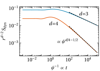
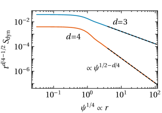
Figure 2: Auxiliary function $\mathcal{S}_{\text{dyn}}(r,t)$ [Eq. 57] as function of (a) time $t$ and (b) distance $r$ for spatial dimensions $d=3$ and $d=4$. $\mathcal{S}_{\text{dyn}}(r,t/2)$ represents the equilibrium two-time correlation function in the bulk [see Eq. 52]. $\mathcal{S}_{\text{dyn}}$ is multiplied by appropriate prefactors which render it a dimensionless function of $\psi=r^{4}/(512t)$ with $t=\gamma{\tilde{t}}$. The actual time and distance dependences are expressed in terms of the dimensionless scaling variable $\psi$ [Eq. 58]. The dashed lines represent the asymptotic behaviors applying to (a) late times [Eq. 60 and (b) large distances [Eq. 59].

We now turn to the auxiliary function $\mathcal{S}_{\text{rel}}$ [Eq. 49b], which can be interpreted as the bulk Green function for the linearized model B [see Eq. 51]. At bulk criticality ($\tau=0$), its real-space expression is given by

$$\begin{split}\mathcal{S}_{\text{rel}}(\mathbf{r},t)&\equiv\frac{1}{\tau_{0}}\int\frac{\mathrm{d}^{d}q}{(2\pi)^{d}}e^{-2\mathbf{q}^{4}t}e^{\mathrm{i}\mathbf{q}\cdot\mathbf{r}}\\ &=\frac{2^{d/2}\pi^{1/2-d/2}}{\Gamma[(2+d)/4]\tau_{0}r^{d}}\psi^{d/4}\Big{[}\,{}_{0}F_{2}\left(\frac{1}{2},\frac{1}{2}+\frac{d}{4};\psi\right)-\frac{2\sqrt{\psi}\Gamma[(2+d)/4]}{\Gamma(1+d/4)}\,{}_{0}F_{2}\left(\frac{3}{2},1+\frac{d}{4};\psi\right)\Big{]}.\end{split}$$ (61)

This result can be readily obtained from Eq. 57 using the relation $\tau_{0}\,\mathcal{S}_{\text{rel}}=-\nabla^{2}\mathcal{S}_{\text{dyn}}$ (with $\tau_{0}=1/v$), which follows directly from the Fourier representations of $\mathcal{S}_{\text{dyn}}$ and $\mathcal{S}_{\text{rel}}$. Due to translational invariance one has $\mathcal{S}_{\text{rel}}(\mathbf{r},t)=\mathcal{S}_{\text{rel}}(r,t)$. For $t\to\infty$ (and any $r\geq 0$) as well as for $r\to 0$ (at fixed $t>0$), $\mathcal{S}_{\text{rel}}$ behaves asymptotically as

$$\mathcal{S}_{\text{rel}}(r\neq 0,t\to\infty)\simeq\mathcal{S}_{\text{rel}}(r\to 0,t>0)\simeq\frac{2^{-7d/4}\pi^{(1-d)/2}}{\tau_{0}\Gamma[1/2+d/4]}t^{-d/4}.$$ (62)

In order to determine the leading behavior of $\mathcal{S}_{\text{rel}}(r,t)$ in the limit $r\to\infty$ for $t>0$ or, equivalently, in the limit $t\to 0$ for $r>0$, the subdominant asymptotics of the generalized hypergeometric function ${}_{0}F_{2}$ is required (see §5.11.2 in Ref. Luke (1969)). One obtains

$$\mathcal{S}_{\text{rel}}(r\to\infty,t>0)\simeq\mathcal{S}_{\text{rel}}(r>0,t\to 0)\simeq\frac{2^{1+d/2}}{\tau_{0}\pi^{d/2}\sqrt{3}\,r^{d}}\psi^{d/6}\exp\left(-\frac{3\psi^{1/3}}{2}\right)\cos[(d\pi-9\sqrt{3}\psi^{1/3})/6].$$ (63)

This shows that $\mathcal{S}_{\text{rel}}$ vanishes in an exponentially damped oscillatory fashion at large distances or short times, respectively. From the Fourier representation in Eq. 61 one infers that the divergence for $t\to 0$ of the expression in Eq. 62 turns, for $t=0$, into $\mathcal{S}_{\text{rel}}(\mathbf{r},t=0)=\tau_{0}^{-1}\delta^{(d)}(\mathbf{r})$. Figure 3 summarizes the behavior of $\mathcal{S}_{\text{rel}}$.

The above expressions for $\mathcal{S}_{\text{dyn}}$ and $\mathcal{S}_{\text{stat}}$ are valid for $d\neq 2$ . In two dimensions, the static correlation function, obtained as the fundamental solution of the Laplace equation, is given by the dimensionless expression $\mathcal{S}_{\text{stat}}=-\ln(r/\ell)/(2\pi)$ with some regularization length scale $\ell$ Le Bellac (1991). The two-dimensional case requires a careful treatment of the logarithmic divergences at short and large wavelengths and is not considered here further.

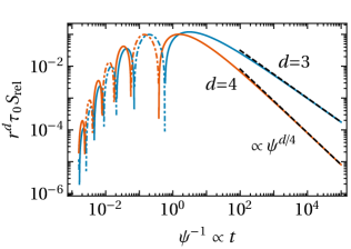
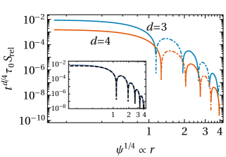
Figure 3: Auxiliary function $\mathcal{S}_{\text{rel}}(r,t)$ [Eq. 61] as function of (a) time $t$ and (b) distance $r$ for spatial dimensions $d=3$ and $d=4$. $\mathcal{S}_{\text{rel}}(r,t/2)$ is proportional to the Green function for the linear model B [see Eq. 51]. $\mathcal{S}_{\text{rel}}$ is multiplied by appropriate prefactors which render it a dimensionless function of $\psi=r^{4}/(512t)$ with $t=\gamma{\tilde{t}}$. The actual time and distance dependences are expressed in terms of the dimensionless scaling variable $\psi$ [Eq. 58]. The dashed-dotted parts correspond to $-\mathcal{S}_{\text{rel}}$. The dashed lines represent the asymptotic behaviors applying to (a) late times [Eq. 62 and (b) large distances [Eq. 63]. For better visibility, the latter asymptote is compared with $\mathcal{S}_{\text{rel}}$ for $d=3$ (solid curve) separately in the inset.

III.2 Equal-time bulk correlation functions

III.2.1 Flat initial conditions

For flat ICs [Eq. 2] the equal-time OP correlator in the bulk $\mathcal{C}_{b}$ [Eq. 54] follows from Eq. 50a:

$$\mathcal{C}_{b}(r,t)=\mathcal{S}_{\text{flat}}(r,t)\equiv\mathcal{S}_{\text{stat}}(r)-\mathcal{S}_{\text{dyn}}(r,t).$$ (64)

Using Eqs. 57 and 59 it can be shown that $\mathcal{S}_{\text{flat}}$ fulfills the scaling behavior expressed in Eq. 8 (with $\mathpzc{c}_{b}\sim(\xi_{+}^{(0)})^{2-d}$ up to numerical constants and within the Gaussian approximation, consistent with Ref. Gambassi and Dietrich (2006)). In particular, $r^{d-2}\mathcal{S}_{\text{flat}}$ is solely a function of the scaling variable $\psi$ [Eq. 58], implying that the asymptotic behaviors of $\mathcal{S}_{\text{flat}}$ for $r\to\infty$ and $t\to 0$ are closely related. The leading asymptotic behavior of $\mathcal{S}_{\text{flat}}$ is given by

$$\mathcal{S}_{\text{flat}}(r\to\infty,t)\simeq\mathcal{S}_{\text{flat}}(r>0,t\to 0)\simeq-\frac{1}{2^{3-d/2}3^{1/2}\pi^{d/2}\,r^{d-2}}\psi^{(d-4)/6}e^{-3\psi^{1/3}/2}\sin\left[\frac{(1-d)\pi}{6}+\frac{3\sqrt{3}}{2}\psi^{1/3}\right],$$ (65)

which follows from the asymptotic behavior of the generalized hypergeometric function ${}_{1}F_{3}$ in next-to-leading order (see §5.11.2 in Ref. Luke (1969)). According to Eq. 60, $\mathcal{S}_{\text{dyn}}$ approaches $\mathcal{S}_{\text{stat}}$ algebraically in $t$ for large $t$, such that

$$\mathcal{S}_{\text{flat}}(r,t\to\infty)\simeq\mathcal{S}_{\text{stat}}(r).$$ (66)

This reflects that, in the bulk, equilibrium is established for $t\to\infty$. The behavior of $\mathcal{S}_{\text{flat}}$ for $r\to 0$ is singular. The intermediate result in Eq. 57 can be written as

$$\mathcal{S}_{\text{flat}}(r,t)=\frac{1}{(2\pi)^{d/2}}\,r^{2-d}\int_{0}^{\infty}\mathrm{d}u\left(1-e^{-2u^{4}t/r^{4}}\right)u^{d/2-2}J_{d/2-1}(u).$$ (67)

Next, performing the limit $t\to 0$ for $r>0$ fixed, yields $\mathcal{S}_{\text{flat}}(r,t=0)=0$, which is also expected from Eq. 59. However, for any $t>0$ we can find a sufficiently small $r$ such that the exponential term in the integral in Eq. 67 becomes negligible. This renders the asymptotic behavior

$$\mathcal{S}_{\text{flat}}(r\to 0,t>0)\simeq\frac{1}{4\pi^{d/2}r^{d-2}}\Gamma(d/2-1)=\mathcal{S}_{\text{stat}}(r),$$ (68)

which implies that, for any finite $t>0$, $\mathcal{S}_{\text{flat}}$ diverges $\propto r^{2-d}$ at small $r$. (Determining the auto-correlation function $\mathcal{C}_{b}(\mathbf{r}=\mathbf{0},t,t^{\prime})$ thus requires a suitable regularization in general, and is not considered here further.) The behavior of $\mathcal{S}_{\text{flat}}$ is illustrated in Fig. 4. As shown in the insets, the asymptotic expression in Eq. 65 accurately captures the exponentially damped oscillatory behavior of $\mathcal{S}_{\text{flat}}$ at early times or, correspondingly, at large distances.

As anticipated in the Introduction, the qualitative behavior of a correlation function $\mathcal{C}$ is often characterized in terms of a time-dependent correlation length $\xi(t)$ Amit and Martin-Mayor (2005). In the present case, however, due to Eq. 56, the standard definition of $\xi(t)$ as the second moment of $\mathcal{C}_{b}$, $\xi^{2}(t)=\frac{\int_{V}\mathrm{d}^{d}r\,r^{2}\mathcal{C}_{b}(\mathbf{r},t)}{\int_{V}\mathrm{d}^{d}r\,\mathcal{C}_{b}(\mathbf{r},t)}$, where $V$ is an arbitrary but sufficiently large volume, is ill-defined. This definition of $\xi^{2}(t)$ is problematic even if one restricts the integral to a lower-dimensional plane: since, for model B, $\mathcal{C}_{b}(r,t)$ is typically decaying in an oscillatory way, one could obtain $\xi^{2}<0$. Instead, a more suitable measure of the growth of the correlation volume is provided by the first zero-crossing $\xi_{\times}$ of $\mathcal{C}_{b}$. Applying this criterion to $\mathcal{S}_{\text{flat}}$, the asymptote in Eq. 65 renders

$$\xi_{\times}\propto t^{1/4},$$ (69)

which is consistent with the dynamic scaling hypothesis for model B in the Gaussian limit Hohenberg and Halperin (1977). The same scaling emerges also for an effective $\xi$ which is defined on the basis of the asymptotic exponential decay reported in Eq. 65.

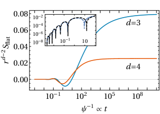
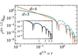
Figure 4: Bulk correlation function $\mathcal{S}_{\text{flat}}(r,t)$ for flat ICs [Eq. 64], as function of (a) time $t$ and (b) distance $r$ for spatial dimensions $d=3$ and $d=4$. $\mathcal{S}_{\text{flat}}$ is multiplied by appropriate prefactors which render it a dimensionless function of $\psi=r^{4}/(512t)$ with $t=\gamma{\tilde{t}}$. The actual time and distance dependences are expressed in terms of the dimensionless scaling variable $\psi$ [Eq. 58]. The dashed-dotted parts correspond to $-\mathcal{S}_{\text{flat}}$. In the insets, $\mathcal{S}_{\text{flat}}$ (for $d=3$) is compared with the asymptotic expression in Eq. 65 (black dashed curve), which captures the exponentially damped oscillatory behavior of $\mathcal{S}_{\text{flat}}$ at early times or large distances, respectively.

III.2.2 Thermal initial conditions

In the case of thermal ICs [Eq. 1], the bulk correlation function is given according to Eq. 50b by

$$\mathcal{C}_{b}(r,t)=\mathcal{S}_{\text{th}}(r,t)=\mathcal{S}_{\text{rel}}(r,t)+\mathcal{S}_{\text{flat}}(r,t).$$ (70)

From Eqs. 57, 59, and 61 it follows that $\mathcal{S}_{\text{th}}$ fulfills the scaling behavior expressed in Eq. 9 (with $\mathpzc{c}_{b}\sim(\xi_{+}^{(0)})^{2-d}$ up to numerical constants and within the Gaussian approximation). Since, at late times, $\mathcal{S}_{\text{flat}}$ approaches $\mathcal{S}_{\text{stat}}$ [see Eq. 66] while $\mathcal{S}_{\text{rel}}$ vanishes [see Eq. 62], the late-time behavior of $\mathcal{S}_{\text{th}}$ is always dominated by $\mathcal{S}_{\text{flat}}$. Furthermore, owing to Eq. 49b, one has $\mathcal{S}_{\text{rel}}\propto 1/\tau_{0}$, such that, in the limit of a large initial temperature, i.e., $\tau_{0}\to\infty$ [see Eq. 48], one obtains $\mathcal{S}_{\text{th}}\simeq\mathcal{S}_{\text{flat}}$. We recall that, in fact, thermal ICs accurately describe an initial equilibrium state only in this limit $\tau_{0}\to\infty$ [see the discussion around Eq. 48].

IV Correlation functions in confinement

In the following, we focus on the equal-time correlation function $\mathcal{C}(\mathbf{r}_{\parallel},z,z^{\prime},t)\equiv\mathcal{C}(\mathbf{r}_{\parallel}-\mathbf{r}_{\parallel}^{\prime},z,z^{\prime},t,t^{\prime}=t)$ of a finite $d$-dimensional system having a cuboidal box geometry. Since we assume periodic BCs in the subspace containing $\mathbf{r}_{\parallel}$ (see Fig. 1), $\mathcal{C}$ is translationally invariant in $\mathbf{r}_{\parallel}$. This is important for determining critical Casimir forces. The thin film limit is readily obtained from the results for a box, as discussed below. We recall that, at finite times $t$, the expression in Eq. 43 for the mode correlations $\langle|a_{n}(\mathbf{p},t)|^{2}\rangle$ applies to all modes including the zero mode $a_{0}(\mathbf{0},t)$. [This is not the case in the limit $t\to\infty$, see the discussion around Eq. 44.] Accordingly, we obtain

$$\mathcal{C}(\mathbf{r}_{\parallel},z,z^{\prime},t)=\frac{1}{A}\sum_{\mathbf{n}_{\parallel},n_{d}}e^{\mathrm{i}\mathbf{p}_{\mathbf{n}_{\parallel}}\cdot\mathbf{r}_{\parallel}}\sigma_{n_{d}}(z)\sigma_{n_{d}}^{*}(z^{\prime})\langle|a_{n_{d}}(\mathbf{p}_{\mathbf{n}_{\parallel}},t)|^{2}\rangle,$$ (71)

where the eigenfunctions $\sigma_{n}$ are given in Eq. 25 and the notation is explained in Eqs. 29 and 30. Applying the Poisson resummation formula [see Eqs. 141 and 142 in Appendix A] renders

$$\mathcal{C}(\mathbf{r}_{\parallel},z,z^{\prime},t)=\mathcal{N}\sum_{\{m_{\alpha}=-\infty\}}^{\{\infty\}}\int\frac{\mathrm{d}^{d}q}{(2\pi)^{d}}e^{\mathrm{i}\mathbf{q}_{\parallel}\cdot\mathbf{r}_{\parallel}+\mathbf{q}\cdot\tilde{\bm{\mathcal{L}}}(\mathbf{m})}\hat{\sigma}_{q_{d}}(z)\hat{\sigma}_{q_{d}}^{*}(z^{\prime})\langle|a(\mathbf{q},t)|^{2}\rangle,$$ (72)

where we use the notation $\sum_{\{m_{\alpha}=-\infty\}}^{\{\infty\}}\equiv\sum_{m_{1}=-\infty}^{\infty}\cdots\sum_{m_{d}=-\infty}^{\infty}$ and define

$$\mathcal{N}^{\text{(p)}}=1,\qquad\hat{\sigma}_{q_{d}}^{\text{(p)}}(z)=e^{\mathrm{i}q_{z}z},$$ (73a)

$$\mathcal{N}^{\text{(N)}}=2,\qquad\hat{\sigma}_{q_{d}}^{\text{(N)}}(z)=\cos(q_{d}z),$$ (73b)

for periodic and Neumann BCs, respectively. Furthermore, the vector $\mathbf{q}$ is decomposed into lateral and transverse components as $\mathbf{q}=\{\mathbf{q}_{\parallel},q_{d}\}$, while $\tilde{\bm{\mathcal{L}}}(\mathbf{m})$ stands for the $d$-dimensional vector

$$\tilde{\bm{\mathcal{L}}}(\mathbf{m})\equiv\{m_{1}L_{\parallel},\ldots,m_{d-1}L_{\parallel},\mathcal{N}m_{d}L\},$$ (74)

which, for $\mathcal{N}=1$ (periodic BCs), we shall simply write as $\bm{\mathcal{L}}(\mathbf{m})$. The notation $a(\mathbf{q},t)$ indicates the continuum case, as explained in Sec. III.

For periodic BCs, Eq. 72 reduces to

$$\mathcal{C}^{\text{(p)}}(\mathbf{r}_{\parallel},z-z^{\prime},t,L)\equiv\mathcal{C}^{\text{(p)}}(\mathbf{r}_{\parallel},z,z^{\prime},t,L)=\sum_{\{m_{\alpha}=-\infty\}}^{\{\infty\}}\mathcal{C}_{b}(\{\mathbf{r}_{\parallel},z-z^{\prime}\}+\bm{\mathcal{L}}(\mathbf{m}),t),$$ (75)

where $\mathcal{C}_{b}$ denotes the (equal-time) bulk correlation function [see Eq. 54]. For Neumann BCs, instead, using

$$\cos(qz)\cos(qz^{\prime})=\frac{1}{2}\left[\cos(q(z-z^{\prime}))+\cos(q(z+z^{\prime}))\right],$$ (76)

Eq. 72 turns into (see also Ref. Diehl and Chamati (2009))

$$\begin{split}\mathcal{C}^{\text{(N)}}(\mathbf{r}_{\parallel},z,z^{\prime},t,L)&=\frac{1}{2}\sum_{\{m_{\alpha}=-\infty\}}^{\{\infty\}}\Big{[}\mathcal{C}_{b}(\{\mathbf{r}_{\parallel},z-z^{\prime}\}+\tilde{\bm{\mathcal{L}}}(\mathbf{m}),t)+\mathcal{C}_{b}(\{\mathbf{r}_{\parallel},-(z-z^{\prime})\}+\tilde{\bm{\mathcal{L}}}(\mathbf{m}),t)\\ &\qquad+\mathcal{C}_{b}(\{\mathbf{r}_{\parallel},z+z^{\prime}\}+\tilde{\bm{\mathcal{L}}}(\mathbf{m}),t)+\mathcal{C}_{b}(\{\mathbf{r}_{\parallel},-(z+z^{\prime})\}+\tilde{\bm{\mathcal{L}}}(\mathbf{m}),t)\Big{]}\\ &=\sum_{\{m_{\alpha}=-\infty\}}^{\{\infty\}}\left[\mathcal{C}_{b}(\{\mathbf{r}_{\parallel},z-z^{\prime}\}+\tilde{\bm{\mathcal{L}}}(\mathbf{m}),t)+\mathcal{C}_{b}(\{\mathbf{r}_{\parallel},z+z^{\prime}\}+\tilde{\bm{\mathcal{L}}}(\mathbf{m}),t)\right]\\ &=\mathcal{C}^{\text{(p)}}(\mathbf{r}_{\parallel},z-z^{\prime},t,2L)+\mathcal{C}^{\text{(p)}}(\mathbf{r}_{\parallel},z+z^{\prime},t,2L),\end{split}$$ (77)

where we have employed Eq. 75 in order to obtain the final result, which involves the correlation function for periodic BCs in a box of thickness $2L$ . Owing to the periodicity $\mathcal{C}^{\text{(p)}}(\mathbf{r}_{\parallel},z=2L,t,2L)=\mathcal{C}^{\text{(p)}}(\mathbf{r}_{\parallel},z=0,t,2L)$, so that, in the special case $z=z^{\prime}=0$ or $z=z^{\prime}=L$, Eq. 77 reduces to

$$\mathcal{C}^{\text{(N)}}(\mathbf{r}_{\parallel},z=z^{\prime}\in\{0,L\},t,L)=2\sum_{\{m_{\alpha}=-\infty\}}^{\{\infty\}}\mathcal{C}_{b}(\{\mathbf{r}_{\parallel},0\}+\tilde{\bm{\mathcal{L}}}(\mathbf{m}),t)=2\,\mathcal{C}^{\text{(p)}}(\mathbf{r}_{\parallel},0,t,2L).$$ (78)

This equation applies also to derivatives of $\mathcal{C}^{\text{(N)}}$ with respect to $\mathbf{r}_{\parallel,\alpha}$, $z$, or $z^{\prime}$, noting that $\partial_{z}^{n}\mathcal{C}^{\text{(p)}}(\mathbf{r}_{\parallel},z,t,2L)=0$ for $z\in\{0,2L\}$ and $n$ odd.

In equilibrium, obtained for $t\to\infty$, the zero mode must be treated carefully due to the non-interchangeability of the limits $t\to\infty$ and $\{\mathbf{n}_{\parallel},n_{d}\}\to\bm{0}$ in the expression for the correlation function in Eq. 72 [see Eq. 45 and the associated discussion]. This is reflected by the fact that $\langle|a_{n_{d}}(\mathbf{p}_{\mathbf{n}_{\parallel}})|^{2}\rangle$ given in Eq. 45 is a discontinuous function of $\{\mathbf{n}_{\parallel},n_{d}\}$. Before applying the Poisson resummation formula in the equilibrium case, one must therefore separate the zero mode from the mode sum in Eq. 72, i.e.,

$$\begin{split}\mathcal{C}_{\text{eq}}(\mathbf{r}_{\parallel},z,z^{\prime},L)&=\frac{1}{A}\sideset{}{{}^{\prime}}{\sum}_{\mathbf{n}_{\parallel},n_{d}}e^{\mathrm{i}\mathbf{p}_{\mathbf{n}_{\parallel}}\cdot\mathbf{r}_{\parallel}}\sigma_{n_{d}}(z)\sigma_{n_{d}}^{*}(z^{\prime})\langle|a_{n_{d}}(\mathbf{p}_{\mathbf{n}_{\parallel}})|^{2}\rangle_{\text{eq}}+\left(\frac{\Phi}{AL}\right)^{2}\\ &=\mathcal{C}_{\text{eq,gc}}(\mathbf{r}_{\parallel},z,z^{\prime})-\frac{1}{AL\,\tau},\end{split}$$ (79)

where $\sideset{}{{}^{\prime}}{\sum}$ stands for the sum excluding the single mode $n_{1}=\ldots=n_{d}=0$, $\Phi$ is the total OP [see Eq. 5], and we have used $\chi_{0}(\mathbf{0},\tau)=\tau$ [see Eq. 42]. Furthermore, we have introduced here the grand canonical static equilibrium correlation function

$$\mathcal{C}_{\text{eq,gc}}(\mathbf{r}_{\parallel},z,z^{\prime},L)=\frac{1}{A}\sum_{\mathbf{n}_{\parallel},n_{d}}e^{\mathrm{i}\mathbf{p}_{\mathbf{n}_{\parallel}}\cdot\mathbf{r}_{\parallel}}\sigma_{n_{d}}(z)\sigma_{n_{d}}^{*}(z^{\prime})\frac{1}{\chi_{n_{d}}(\mathbf{p}_{\mathbf{n}_{\parallel}},\tau)}+\left(\frac{\Phi}{AL}\right)^{2},$$ (80)

which does not involve a constraint on the zero mode [see also Eq. 44]. The last term in Eq. 80 is due to the fact that we consider the correlations of the actual OP $\phi$ and not of its fluctuation $\phi-\Phi/(AL)$. (In the present study, we focus on $\Phi=0$.) Since Eq. 79 holds for all BCs considered here, upon applying the Poisson resummation formula to Eq. 80, one obtains the same expression for $\mathcal{C}_{\text{eq,gc}}$ as reported in Eqs. 75 and 77 but with $\mathcal{C}_{b}(\mathbf{r},t)$ replaced by $\mathcal{C}_{b,\text{eq}}(\mathbf{r})$.

Equation 79 coincides with the expression for the correlation function in the canonical ensemble, derived within equilibrium field theory in Ref. Gross et al. (2017). The term $-1/(AL\tau)$ represents the constraint-induced correction stemming from the non-fluctuating character of $\Phi$ [see Eq. 40]. This term diverges at criticality ($\tau\to 0$) and cancels the corresponding divergence of the grand canonical correlation function $\mathcal{C}_{\text{eq,gc}}$ [Eq. 80], such that the canonical one, $\mathcal{C}_{\text{eq}}$ [Eq. 79], stays finite for $\tau\to 0$ .

In the case of a thin film, where the transverse area $A=L_{\parallel}^{d-1}\to\infty$ is infinitely extended, the $(d-1)$-dimensional sum over $\mathbf{p}_{n}$ in Eq. 71 has to be replaced according to

$$\frac{1}{A}\sum_{\mathbf{n}}f(\mathbf{p}_{\mathbf{n}})\to\int\frac{\mathrm{d}^{d-1}p}{(2\pi)^{d-1}}f(\mathbf{p}).$$ (81)

Consequently, the associated Poisson representation of the correlation function in Eq. 72 involves only the sum over $m_{z}$, such that Eqs. 75, 77, and 78 reduce to

$$\mathcal{C}^{\text{(p)}}(\mathbf{r}_{\parallel},z-z^{\prime},t,L) =\sum_{m=-\infty}^{\infty}\mathcal{C}_{b}(\{\mathbf{r}_{\parallel},z-z^{\prime}+mL\},t),$$ (82a)

$$\mathcal{C}^{\text{(N)}}(\mathbf{r}_{\parallel},z,z^{\prime},t,L) =\sum_{m=-\infty}^{\infty}\left[\mathcal{C}_{b}(\{\mathbf{r}_{\parallel},z-z^{\prime}+2mL\},t)+\mathcal{C}_{b}(\{\mathbf{r}_{\parallel},z+z^{\prime}+2mL\},t)\right],$$ (82b)

$$\mathcal{C}^{\text{(N)}}(\mathbf{r}_{\parallel},z=z^{\prime}\in\{0,L\},t,L) =2\sum_{m=-\infty}^{\infty}\mathcal{C}_{b}(\{\mathbf{r}_{\parallel},2mL\},t)=2\,\mathcal{C}^{\text{(p)}}(\mathbf{r}_{\parallel},0,t,2L).$$ (82c)

Further analytic expressions for these correlation functions are provided in Appendix B. Importantly, the constraint-induced correction $-1/(AL\tau)$ vanishes in Eq. 79 both in the thin film limit and in the bulk limit, implying that the corresponding correlation function is identical in the canonical and grand canonical ensembles:

$$\mathcal{C}_{\text{eq}}(\mathbf{r}_{\parallel},z,z^{\prime})=\mathcal{C}_{\text{eq,gc}}(\mathbf{r}_{\parallel},z,z^{\prime}),\qquad\text{($A\to\infty$ or $V\to\infty$)}.$$ (83)

We note, however, that this property is specific to non-symmetry-breaking BCs, while, for symmetry-breaking BCs, in a thin film Gross et al. (2016) ensemble differences can be relevant.

V Critical Casimir force

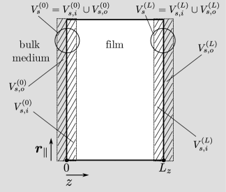
Figure 5: Schematic view of the system under consideration, projected onto one of the lateral dimensions. The hatched areas represent the integration volumes $V_{s}^{(0,L)}$ around the surfaces at $z=0$ and $z=L$, entering into Eq. 85, while the shaded area illustrates the bulk medium at the outside. The thickness of $V_{s}$ is taken to be infinitesimal, which facilitates the use of no-flux BCs [or, correspondingly, the symmetry of the in-going and out-going fluxes in the case of periodic BCs; see the discussion after Eq. 89]. $V_{s,\{i,o\}}^{(0,L)}$ denotes the volumes of the inner/outer fluid at the wall at $z=0$ and $z=L$, respectively; $V_{s}^{(0,L)}=V_{s,i}^{(0,L)}\cup V_{s,o}^{(0,L)}$.

Following Refs. Dean and Gopinathan (2010); Rohwer et al. (2017, 2018); Krüger et al. (2018); Gross et al. (2018), we define the CCF in terms of the generalized force exerted by the OP field on an inclusion (e.g., a surface) in the system. For a given instantaneous (i.e., spatially varying, but fixed) field configuration $\phi(\mathbf{r})$, the generalized force acting in direction $i$ on a single surface described by an energy density $\mathcal{H}_{s}(l_{i},\phi(\mathbf{r}))$ localized at $r_{i}=l_{i}$ is defined by Dean and Gopinathan (2010); Krüger et al. (2018); Gross et al. (2018)

$$K_{i}\equiv-\frac{\partial\mathcal{F}}{\partial l_{i}}=-\int_{V}\mathrm{d}^{d}r\frac{\partial\mathcal{H}(\mathbf{r},\phi(\mathbf{r}),\nabla\phi(\mathbf{r}))}{\partial l_{i}}.$$ (84)

Here, $\mathcal{F}=\int_{V}\mathrm{d}^{d}r\,\mathcal{H}$ denotes the total energy, with $\mathcal{H}=\mathcal{H}_{b}+\mathcal{H}_{s}$ and the bulk energy density $\mathcal{H}_{b}$ [see Eq. 18]. $V$ is the system volume independent of $l_{i}$. In the case of the bounding surfaces of the system, located at $z=L$ and $z=0$, respectively, the generalized force $K_{i}$ in direction $i=z$ can be expressed as Krüger et al. (2018); Gross et al. (2018)

$$K_{i}^{(L)} =-\int_{\partial V_{s}^{(L)}}\mathrm{d}^{d-1}s_{j}\,\bar{\mathcal{T}}_{ij}+\int_{V_{s}^{(L)}}\mathrm{d}^{d}r\,(\nabla_{i}\mu)\phi\,,$$ (85a)

$$K_{i}^{(0)} =+\int_{\partial V_{s}^{(0)}}\mathrm{d}^{d-1}s_{j}\,\bar{\mathcal{T}}_{ij}-\int_{V_{s}^{(0)}}\mathrm{d}^{d}r\,(\nabla_{i}\mu)\phi\,,$$ (85b)

where $V_{s}^{(0)}$ and $V_{s}^{(L)}$ are cuboid-shaped volumes of infinitesimal thickness enclosing the surfaces at $z=L$ and $z=0$, respectively (see Fig. 5),

$$\bar{\mathcal{T}}_{ij}\equiv\mathcal{T}_{ij}+\mu\phi\delta_{ij}$$ (86)

defines the dynamical stress tensor,

$$\mathcal{T}_{ij}=\frac{\partial\mathcal{H}}{\partial\nabla_{i}\phi}\nabla_{j}\phi-\delta_{ij}\mathcal{H}$$ (87)

is the standard (grand canonical) stress tensor Krech (1994), and

$$\mu=\frac{\delta\mathcal{F}}{\delta\phi}=\frac{\partial\mathcal{H}}{\partial\phi}-\nabla_{j}\left(\frac{\partial\mathcal{H}}{\partial\nabla_{j}\phi}\right)$$ (88)

is the chemical potential. The different signs in Eq. 85 stem from the symmetrization of the derivative with respect to $l_{z}$ in Eq. 84, which is necessary in order to obtain equal but opposite forces on the boundaries of the system (see Ref. Gross et al. (2018)). The above expressions apply for any generic $\mathcal{H}_{b}$ which is at most quadratic in gradients of $\phi$, but can contain arbitrary powers of $\phi$.

The generalized force $K_{z}$ (per area $A$), averaged over the left and right boundary of the system, renders the dynamic CCF $\mathcal{K}$:

$$\mathcal{K}=\frac{1}{2A}\left(K_{z}^{(0)}+K_{z}^{(L)}\right).$$ (89)

Upon thermal averaging, the first term on the r.h.s. of Eq. 85 provides identical contributions to $\mathcal{K}$ at the two boundaries. If $\phi$ as well as the noise [see Eq. 21] obey no-flux BCs at the surfaces, the second term on the r.h.s. of Eq. 85 vanishes due to the infinitesimal thickness of $V_{s}$. In fact, in this case, the symmetrized definition in Eq. 89 is not necessary. For periodic BCs, instead, non-vanishing fluxes across the surfaces imply that the last term in Eq. 85 does not vanish at any single boundary. However, we have $\nabla_{i}\mu|_{z=0}=\nabla_{i}\mu|_{z=L}$, such that the last term on the r.h.s. of Eq. 85 cancels in the sum in Eq. 89. We note that, in thermal equilibrium, the second term on the r.h.s. of Eq. 85 is zero on average, i.e., $\langle(\nabla_{i}\mu)\phi\rangle=0$ [see Eq. 117 below and Ref. Dean and Gopinathan (2010)].

Taking into account the direction of the surface normals (which point outward from the respective volumes $V_{s}$), the mean CCF follows from Eqs. 85 and 89 as

$$\begin{split}\langle\mathcal{K}(t)\rangle&=\frac{1}{A}\int_{\partial V^{(L,0)}_{s,i}}\mathrm{d}^{d-1}s^{(L,0)}_{z}(\mathbf{r}_{\parallel},z)\,\langle\bar{\mathcal{T}}_{zz}(\mathbf{r}_{\parallel},z,t)\rangle-\frac{1}{A}\int_{\partial V^{(L,0)}_{s,o}}\mathrm{d}^{d-1}s^{(L,0)}_{z}(\mathbf{r}_{\parallel},z)\,\langle\bar{\mathcal{T}}_{zz,b}(\mathbf{r}_{\parallel},z,t)\rangle\\ &\equiv\langle\mathcal{P}_{f}(t)\rangle-\langle\mathcal{P}_{b}(t)\rangle,\end{split}$$ (90)

where $\partial V^{(L,0)}_{s,\{i,o\}}$ denotes the surface of the inner/outer fluid at $z=L$ and $z=0$, respectively (see Fig. 5) [with the corresponding area element $\mathrm{d}^{d-1}s_{z}(\mathbf{r}_{\parallel},z)$], and where $\bar{\mathcal{T}}_{zz,b}$, accordingly, represents the bulk stress. As set out in Eq. 11, the last line in Eq. 90 defines the averaged film and bulk pressures. We shall use the notion of a film pressure both in the case of a thin film and that of a box geometry.

For a Gaussian Hamiltonian density of the Landau-Ginzburg form [Eq. 18], the chemical potential [Eq. 88] reduces to the bulk value $\mu=-\nabla^{2}\phi+\tau\phi$ and the dynamic stress tensor in Eq. 86 takes the form

$$\bar{\mathcal{T}}_{zz}=\frac{1}{2}(\partial_{z}\phi)^{2}-\frac{1}{2}\sum_{\alpha=1}^{d-1}(\partial_{\alpha}\phi)^{2}+\frac{1}{2}\tau\phi^{2}-\phi\nabla^{2}\phi.$$ (91)

In the following, we focus on a critical quench, i.e., $\tau=0$; as before, we also assume $\Phi=0$. Accordingly, the mean CCF in Eq. 90 is given by

$$\begin{split}\langle\mathcal{K}(t)\rangle&=\langle\mathcal{P}_{f}(t)\rangle-\langle\mathcal{P}_{b}(t)\rangle\\ &=\Bigg{[}\frac{1}{2}\langle(\partial_{z}\phi(\mathbf{r}_{\parallel},z,t))^{2}\rangle-\langle\phi(\mathbf{r}_{\parallel},z,t)\partial_{z}^{2}\phi(\mathbf{r}_{\parallel},z,t)\rangle-\frac{1}{2}\sum_{\alpha=1}^{d-1}\langle(\partial_{\alpha}\phi(\mathbf{r}_{\parallel},z,t))^{2}\rangle\\ &\quad-\Big{\langle}\phi(\mathbf{r}_{\parallel},z,t)\sum_{\alpha=1}^{d-1}\partial_{\alpha}^{2}\phi(\mathbf{r}_{\parallel},z,t)\Big{\rangle}\Bigg{]}_{{\mathbf{r}_{\parallel}=\mathbf{0}_{\parallel}}\atop{z\in\{0,L\}}}-\text{(bulk)},\end{split}$$ (92)

where ‘(bulk)’ denotes the corresponding bulk contribution, explicit expressions of which will be provided below. In Eq. 92, translational invariance along the lateral directions allows one to set $\mathbf{r}_{\parallel}=\mathbf{0}$. The correlations of the OP derivatives can be cast into derivatives of the OP correlation function, as will be shown below.

Here we emphasize that Eq. 92 strictly applies only to finite times. In fact, upon taking the limit $t\to\infty$ in order to calculate equilibrium quantities, it is necessary to regularize the zero-mode divergence occurring for $\tau\to 0$ [see Eqs. 79 and 83 and the associated discussion]. Accordingly, in the case $t\to\infty$, a nonzero $\tau>0$ must be kept within the intermediate calculations and the limit $\tau\to 0$ is carried out only at the end. An exception is a thin film ($\varrho=0$) where, within Gaussian approximation, the zero-mode divergence does not play a role because the corresponding problematic term in Eq. 79 vanishes Gross et al. (2017) . For a thin film, one may thus set $\tau=0$ from the outset if one takes the limit $t\to\infty$.

We proceed by analyzing the dynamical and equilibrium CCF for various geometries and BCs based on the stress tensor formalism.

V.1 Thin film with periodic BCs

We first consider a thin film with periodic BCs at its confining surfaces ($z=0,L$), which is the simplest geometry to study CCFs. Using Eq. 72 [reduced to the special case of a thin film via Eq. 81], we determine the following auto-correlators:

$$\langle\mathcal{R}^{\text{(p)}}(t)\rangle \equiv\langle\partial_{z}\phi(\mathbf{0}_{\parallel},z,t)\partial_{z}\phi(\mathbf{0}_{\parallel},z,t)\rangle\big{|}_{z\in\{0,L\}}=\frac{1}{L}\int\frac{\mathrm{d}^{d-1}p}{(2\pi)^{d-1}}\sum_{n}(\lambda_{n}^{\text{(p)}})^{2}\langle|a_{n}(\mathbf{p},t)|^{2}\rangle$$

$$=-\langle\phi(\mathbf{0}_{\parallel},z,t)\partial_{z}^{2}\phi(\mathbf{0}_{\parallel},z,t)\rangle\big{|}_{z\in\{0,L\}}=-\partial_{z}^{2}\mathcal{C}^{\text{(p)}}(\mathbf{0}_{\parallel},z,t)\big{|}_{z=0},$$ (93a)

$$\langle\mathcal{Q}^{\text{(p)}}(t)\rangle \equiv\Big{\langle}\phi(\mathbf{r}_{\parallel},z,t)\nabla_{\parallel}^{2}\phi(\mathbf{r}_{\parallel},z,t)\Big{\rangle}\Big{|}_{{\mathbf{r}_{\parallel}=\mathbf{0}_{\parallel}}\atop{z\in\{0,L\}}}=-\frac{1}{L}\int\frac{\mathrm{d}^{d-1}p}{(2\pi)^{d-1}}\sum_{n}\mathbf{p}^{2}\langle|a_{n}(\mathbf{p},t)|^{2}\rangle$$

$$=-\sum_{a=1}^{d-1}\langle(\partial_{\alpha}\phi(\mathbf{r}_{\parallel},z,r))^{2}\rangle\Big{|}_{{\mathbf{r}_{\parallel}=\mathbf{0}_{\parallel}}\atop{z\in\{0,L\}}}=\nabla_{\parallel}^{2}\mathcal{C}^{\text{(p)}}(\mathbf{r}_{\parallel},0,t)\big{|}_{\mathbf{r}_{\parallel}=\mathbf{0}_{\parallel}},$$ (93b)

where we have introduced the operator

$$\nabla_{\parallel}^{2}\equiv\sum_{\alpha=1}^{d-1}\partial_{\alpha}^{2}.$$ (94)

The averaged instantaneous film pressure $\langle\mathcal{P}_{f}\rangle$ follows according to Eq. 92 as

$$\langle\mathcal{P}_{f}^{\text{(p)}}(t)\rangle=\frac{3}{2}\langle\mathcal{R}^{\text{(p)}}(t)\rangle-\frac{1}{2}\langle\mathcal{Q}^{\text{(p)}}(t)\rangle.$$ (95)

Upon applying the Poisson resummation formula via Eq. 82a (see also Appendix A), one obtains

$$\langle\mathcal{R}^{\text{(p)}}(t)\rangle =-\sum_{m=-\infty}^{\infty}\partial_{z}^{2}\mathcal{C}_{b}(\{\mathbf{0}_{\parallel},z\},t)\big{|}_{z=Lm},$$ (96a)

$$\langle\mathcal{Q}^{\text{(p)}}(t)\rangle =\sum_{m=-\infty}^{\infty}\nabla_{\parallel}^{2}\mathcal{C}_{b}(\{\mathbf{r}_{\parallel},z\},t)\big{|}_{z=Lm,\,\mathbf{r}_{\parallel}=\mathbf{0}_{\parallel}},$$ (96b)

in terms of the equal-time bulk correlation function $\mathcal{C}_{b}$ defined in Eq. 54.

In the following we consider flat as well as thermal ICs, for which the bulk correlator $\mathcal{C}_{b}$ is provided in Eqs. 64 and 70, respectively. The derivatives required in Eq. 96 are readily obtained from the analytic expressions for $\mathcal{C}_{b}$ provided in Sec. III. Since $\mathcal{C}_{b}$ depends only on $r=|\mathbf{r}|$, one has

$$\partial_{\alpha}^{2}\mathcal{C}_{b}(r,t)=\partial_{\alpha}\left[\frac{r_{\alpha}}{r}\,\partial_{r}\mathcal{C}_{b}(r,t)\right]=\frac{r_{\alpha}^{2}}{r^{2}}\partial_{r}^{2}\mathcal{C}_{b}(r,t)+\left(\frac{1}{r}-\frac{r_{\alpha}^{2}}{r^{3}}\right)\partial_{r}\mathcal{C}_{b}(r,t).$$ (97)

Consequently Eq. 96b can be written as $\langle\mathcal{Q}^{\text{(p)}}(t)\rangle=\sum_{m=-\infty}^{\infty}\frac{d-1}{z}\partial_{z}\mathcal{C}_{b}(\{\mathbf{0}_{\parallel},z\},t)\big{|}_{z=Lm}$. Explicit expressions for the derivatives of $\mathcal{S}_{\text{dyn}}$ and $\mathcal{S}_{\text{rel}}$ are rather lengthy, and are not stated here; they can be readily obtained from Eqs. 57 and 61 using standard properties of hypergeometric functions Olver et al. (2010). However, it is useful to report the following asymptotic behaviors ($\beta=1,\ldots,d$):

$$\partial_{r}^{2}\mathcal{S}_{\text{dyn}}(r,t\to\infty) \simeq\partial_{r}^{2}\mathcal{S}_{\text{dyn}}(r,t)\big{|}_{z\to 0}\simeq\partial_{\beta}^{2}\mathcal{S}_{\text{dyn}}(r,t\to\infty)\big{|}_{\mathbf{r}_{\parallel}=\mathbf{0}_{\parallel}}\simeq\partial_{\beta}^{2}\mathcal{S}_{\text{dyn}}(r,t)\big{|}_{\mathbf{r}_{\parallel}=\mathbf{0}_{\parallel},\,z\to 0}$$

$$\simeq r^{-1}\partial_{r}\mathcal{S}_{\text{dyn}}(r,t\to\infty)\simeq r^{-1}\partial_{r}\mathcal{S}_{\text{dyn}}(r,t)\big{|}_{r\to 0}$$

$$\simeq-\frac{\Gamma(d/4)}{2^{2+5d/4}\pi^{d/2}\Gamma(1+d/2)t^{d/4}},$$ (98a)

$$\partial_{r}^{2}\mathcal{S}_{\text{rel}}(r\neq 0,t\to\infty) \simeq r^{-1}\partial_{r}\mathcal{S}_{\text{rel}}(r\neq 0,t\to\infty)\simeq-\frac{\pi^{1/2-d/2}}{2^{5/2+7d/4}\Gamma(1+d/4)\,t^{1/2+d/4}},$$ (98b)

$$\partial_{r}^{2}\mathcal{S}_{\text{rel}}(r\neq 0,t\to 0) \sim r^{-1}\partial_{r}\mathcal{S}_{\text{rel}}(r\neq 0,t\to 0)\sim\partial_{r}^{2}\mathcal{S}_{\text{rel}}(r,t)\big{|}_{r\to\infty}\sim r^{-1}\partial_{r}\mathcal{S}_{\text{rel}}(r,t\to 0)\big{|}_{r\to\infty}\to 0,$$ (98c)

$$\partial_{r}^{2}\mathcal{S}_{\text{flat}}(r,t\to 0) \simeq\partial_{r}^{2}\mathcal{S}_{\text{flat}}(r,t)\big{|}_{r\to\infty}\simeq r^{-1}\partial_{r}\mathcal{S}_{\text{flat}}(r,t\to 0)\simeq r^{-1}\partial_{r}\mathcal{S}_{\text{flat}}(r,t)\big{|}_{r\to\infty}\to 0.$$ (98d)

In fact, according to Eq. 65, $\partial_{r}^{2}\mathcal{S}_{\text{dyn}}$ approaches $\partial_{r}^{2}\mathcal{S}_{\text{stat}}$ exponentially for large $r$ or small $t$. Furthermore, the leading asymptotic behavior extending Eq. 98c to large but finite $r$ or small but nonzero $t$ can be straightforwardly obtained from Eq. 63.

Owing to Eqs. 98c and 98d, the derivatives of $\mathcal{C}_{b}$ appearing in Eq. 96 vanish for $|z|\to\infty$. Therefore in Eq. 96, in the bulk limit $L\to\infty$, only terms for $m=0$ survive. These render, via Eq. 12, the bulk pressure $\langle\mathcal{P}_{b}(t)\rangle$. The bulk pressure can equivalently be obtained by directly evaluating the r.h.s. of Eq. 95 with the bulk correlation function [Eq. 54].

Using the fact that $\mathcal{C}_{b}(z,t)=\mathcal{C}_{b}(-z,t)$, the time-dependent CCF [Eq. 92] at bulk criticality ($\tau=0$) for a slab with periodic BCs eventually follows as

$$\langle\mathcal{K}^{\text{(p)}}(t)\rangle=-\sum_{m=1}^{\infty}\left[3\partial_{z}^{2}\mathcal{C}_{b}(z,t)+\frac{d-1}{z}\partial_{z}\mathcal{C}_{b}(z,t)\right]_{z=Lm}.$$ (99)

Since $\mathcal{C}_{b}$ fulfils the scaling behavior in Eq. 9 with $\mathpzc{z}=4$ [and recalling Eqs. 15 and 22], one readily demonstrates that $\langle\mathcal{K}^{\text{(p)}}(t)\rangle$ indeed has the scaling form anticipated in Eq. 13 (with $\ring{\tau}=0$). In particular, $L^{d}\langle\mathcal{K}^{\text{(p)}}\rangle$ is a function of the dimensionless time scaling variable $t/L{z}$.

V.1.1 Equilibrium CCF

The contributions from $\mathcal{S}_{\text{dyn}}$ and $\mathcal{S}_{\text{rel}}$ vanish in the long-time limit, owing to Eqs. 98b and 98a. Both for flat and thermal ICs [see Eqs. 64 and 70], the equilibrium CCF $\langle\mathcal{K}^{\text{(p)}}\rangle_{\text{eq}}$ at bulk criticality thus follows by inserting $\mathcal{C}_{b}=\mathcal{S}_{\text{stat}}$ [Eq. 59] into Eq. 99, rendering

$$\langle\mathcal{K}^{\text{(p)}}\rangle_{\text{eq}}=\langle\mathcal{K}^{\text{(p)}}(t\to\infty)\rangle=-\sum_{m=1}^{\infty}\left[3\partial_{z}^{2}\mathcal{S}_{\text{stat}}(z)+\frac{d-1}{z}\partial_{z}\mathcal{S}_{\text{stat}}(z)\right]=L^{-d}\pi^{-d/2}\Gamma(d/2)(1-d)\zeta(d),$$ (100)

where, in the last step, we have used Eq. 59 and introduced the Riemann zeta-function $\zeta(s)=\sum_{n=1}^{\infty}n^{-s}$ Olver et al. (2010). In spatial dimensions $d=3$ and $4$, one obtains

$$\langle\mathcal{K}^{\text{(p)}}\rangle_{\text{eq}}=\begin{cases}\displaystyle-\frac{1}{L^{3}}\frac{\zeta(3)}{\pi},\qquad&d=3,\\[12.0pt] \displaystyle-\frac{1}{L^{4}}\frac{\pi^{2}}{30},&d=4,\end{cases}$$ (101)

respectively. The same expression as in Eq. 100 is obtained from a calculation of $\langle\mathcal{K}^{\text{(p)}}\rangle_{\text{eq}}$ based on the residual finite-size free energy (see Ref. Krech and Dietrich (1992)). Note that, concerning the CCF, the ensemble difference is immaterial for a thin film with periodic BCs [see also Eq. 83].

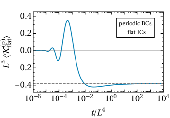
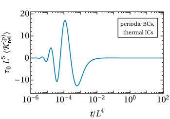
Figure 6: Time evolution of the dynamic CCF $\langle\mathcal{K}^{\text{(p)}}(t)\rangle$ [per $k_{B}T_{c}$, Eq. 99] in a thin film for periodic BCs and $d=3$ dimensions. At time $t=0$, the system is instantaneously quenched to the bulk critical temperature ($\tau=0$). Panel (a) shows the CCF for flat ICs [Eq. 2] and the dashed line indicates the value of the equilibrium CCF at $T_{c}$ [Eq. 100]. Panel (b) shows the contribution $\tau_{0}\langle\mathcal{K}^{\text{(p)}}_{\text{rel}}(t)\rangle$ [Eq. 105] to the CCF $\langle\mathcal{K}^{\text{(p)}}_{\text{th}}(t)\rangle=\langle\mathcal{K}^{\text{(p)}}_{\text{flat}}(t)\rangle+\langle\mathcal{K}^{\text{(p)}}_{\text{rel}}(t)\rangle$ for thermal ICs [Eq. 1], where $\tau_{0}=1/v$ is a measure of the initial temperature [see Eq. 48]. In both panels, CCF and time are scaled according to Eq. 13, such that the universal behavior of the CCF scaling function is exhibited by the plot explicitly.

V.1.2 Dynamic CCF for flat initial conditions

The CCF for flat ICs, which is obtained by inserting $\mathcal{C}_{b}=\mathcal{S}_{\text{flat}}$ [Eq. 64] into Eq. 99, is denoted by $\langle\mathcal{K}^{\text{(p)}}_{\text{flat}}(t)\rangle$. At finite times, a closed analytical expression for $\langle\mathcal{K}^{\text{(p)}}_{\text{flat}}(t)\rangle$ is not available, and the CCF thus has to be determined numerically. Due to the rapid exponential decay of $\mathcal{S}_{\text{flat}}$ for large values of $r$ [see Eq. 65], it suffices to retain only the first few terms of the sum in Eq. 99 in order to obtain an accurate estimate. The CCF $\langle\mathcal{K}^{\text{(p)}}_{\text{flat}}(t)\rangle$ obtained in this way is illustrated in Fig. 6(a) for $d=3$ spatial dimensions. From Eq. 98d it follows that the CCF vanishes initially:

$$\langle\mathcal{K}_{\text{flat}}^{\text{(p)}}(t=0)\rangle=0.$$ (102)

At short times $t/L{z}\lesssim\mathcal{O}(1)$, the CCF grows in an oscillatory fashion. At late times $t/L{z}\gtrsim\mathcal{O}(1)$ the CCF approaches its equilibrium value [Eq. 100] algebraically in time from below (see Appendix C for a derivation of this behavior):

$$\langle\mathcal{K}_{\text{flat}}^{\text{(p)}}(t)\rangle-\langle\mathcal{K}^{\text{(p)}}\rangle_{\text{eq}}\propto-t^{1/4-d/4}.$$ (103)

V.1.3 Dynamic CCF for thermal initial conditions

According to Eq. 70, the dynamic CCF for thermal ICs can be written as

$$\langle\mathcal{K}^{\text{(p)}}_{\text{th}}(t)\rangle=\langle\mathcal{K}^{\text{(p)}}_{\text{rel}}(t)\rangle+\langle\mathcal{K}^{\text{(p)}}_{\text{flat}}(t)\rangle,$$ (104)

where $\langle\mathcal{K}^{\text{(p)}}_{\text{flat}}\rangle$ is defined in the preceding subsection, while

$$\langle\mathcal{K}^{\text{(p)}}_{\text{rel}}(t)\rangle\equiv-\sum_{m=1}^{\infty}\left[3\partial_{z}^{2}\mathcal{S}_{\text{rel}}(z,t)+\frac{2}{z}\partial_{z}\mathcal{S}_{\text{rel}}(z,t)\right]_{z=Lm}$$ (105)

captures the contribution stemming from $\mathcal{S}_{\text{rel}}$ [Eq. 61]. According to Eqs. 98b and 98c, $\langle\mathcal{K}^{\text{(p)}}_{\text{rel}}\rangle$ vanishes both initially and at late times, implying that $\langle\mathcal{K}^{\text{(p)}}_{\text{rel}}\rangle$ essentially modifies only the transient behavior of the dynamic CCF. Since $\langle\mathcal{K}^{\text{(p)}}_{\text{rel}}\rangle\propto 1/\tau_{0}$, for large initial temperatures [see Eq. 48] the influence of the thermal IC is diminished, such that $\langle\mathcal{K}^{\text{(p)}}_{\text{th}}(t)\rangle\big{|}_{\tau_{0}\to\infty}\simeq\langle\mathcal{K}^{\text{(p)}}_{\text{flat}}(t)\rangle$. Figure 6(b) displays $\tau_{0}\langle\mathcal{K}^{\text{(p)}}_{\text{rel}}(t)\rangle$, which is independent of the initial temperature $\tau_{0}$, as function of time.

V.2 Thin film with Neumann BCs

In order to obtain the dynamic CCF in a thin film with Neumann BCs, we proceed as in Sec. V.1. Accordingly, using Eqs. 72 and 81, we obtain the following correlation functions:

$$\langle\mathcal{R}^{\text{(N)}}(t)\rangle \equiv-\langle\phi(\mathbf{0}_{\parallel},z,t)\partial_{z}^{2}\phi(\mathbf{0}_{\parallel},z,t)\rangle\big{|}_{z\in\{0,L\}}=\frac{1}{L}\int\frac{\mathrm{d}^{d-1}p}{(2\pi)^{d-1}}\sum_{n=0}^{\infty}(\lambda_{n}^{\text{(N)}})^{2}(2-\delta_{n,0})\langle|a_{n}(\mathbf{p},t)|^{2}\rangle$$

$$=-\partial_{z}^{2}\mathcal{C}^{\text{(N)}}(\mathbf{r}_{\parallel}=\mathbf{0}_{\parallel},z,z^{\prime},t)\big{|}_{z=z^{\prime}\in\{0,L\}},$$ (106a)

$$\langle\mathcal{Q}^{\text{(N)}}(t)\rangle \equiv\big{\langle}\phi(\mathbf{r}_{\parallel},z,t)\sum_{\alpha=1}^{d-1}\partial_{\alpha}^{2}\phi(\mathbf{r}_{\parallel},z,t)\big{\rangle}\Big{|}_{{\mathbf{r}_{\parallel}=\mathbf{0}_{\parallel}}\atop{z\in\{0,L\}}}=-\sum_{\alpha=1}^{d-1}\langle(\partial_{\alpha}\phi(\mathbf{r}_{\parallel},z,r))^{2}\rangle\Big{|}_{{\mathbf{r}_{\parallel}=\mathbf{0}_{\parallel}}\atop{z\in\{0,L\}}}$$

$$=-\frac{1}{L}\int\frac{\mathrm{d}^{d-1}p}{(2\pi)^{d-1}}\sum_{n=0}^{\infty}\mathbf{p}^{2}(2-\delta_{n,0})\langle|a_{n}(\mathbf{p},t)|^{2}\rangle=\nabla_{\parallel}^{2}\mathcal{C}^{\text{(N)}}(\mathbf{r}_{\parallel},z,z,t)\big{|}_{z\in\{0,L\}},$$ (106b)

in terms of which Eq. 92 renders the film pressure

$$\langle\mathcal{P}_{f}^{\text{(N)}}(t)\rangle=\langle\mathcal{R}^{\text{(N)}}(t)\rangle-\frac{1}{2}\langle\mathcal{Q}^{\text{(N)}}(t)\rangle.$$ (107)

Upon invoking the Poisson summation formula via Eq. 82b (see also Appendix A), the correlators in Eq. 106 can be expressed as

$$\langle\mathcal{R}^{\text{(N)}}(t)\rangle =-2\sum_{m=-\infty}^{\infty}\partial_{z}^{2}\mathcal{C}_{b}(\{\mathbf{r}_{\parallel}=\mathbf{0}_{\parallel},z\},t)\big{|}_{z=2Lm}=2\langle\mathcal{R}^{\text{(p)}}(t)\rangle\big{|}_{L\to 2L},$$ (108a)

$$\langle\mathcal{Q}^{\text{(N)}}(t)\rangle =2\sum_{m=-\infty}^{\infty}\nabla_{\parallel}^{2}\mathcal{C}_{b}(\{\mathbf{r}_{\parallel},z\},t)\big{|}_{z=2Lm,\,\mathbf{r}_{\parallel}=\mathbf{0}_{\parallel}}=2\sum_{m=-\infty}^{\infty}\frac{d-1}{z}\partial_{z}\mathcal{C}_{b}(\{\mathbf{0}_{\parallel},z\},t)\big{|}_{z=2Lm}=2\langle\mathcal{Q}^{\text{(p)}}(t)\rangle\big{|}_{L\to 2L},$$ (108b)

where $\mathcal{C}_{b}$ is the equal-time bulk correlation function [Eq. 54] and where we have used Eq. 97 as well as Eq. 96. On the r.h.s., the expressions for periodic BCs given in Eq. 96 are to be evaluated for $2L$ instead of $L$.

As before, the bulk pressure $\langle\mathcal{P}_{b}^{\text{(N)}}(t)\rangle$ is provided by the terms pertaining to $m=0$ in Eq. 108. Consequently, the dynamic CCF for a film with Neumann BCs follows from Eqs. 107 and 108 as

$$\langle\mathcal{K}^{\text{(N)}}(t)\rangle=-2\sum_{m=1}^{\infty}\left[2\partial_{z}^{2}\mathcal{C}_{b}(z,t)+\frac{d-1}{z}\partial_{z}\mathcal{C}_{b}(z,t)\right]_{z=2Lm}=-2^{-d+1}\sum_{m=1}^{\infty}\left[2\partial_{z}^{2}\mathcal{C}_{b}(z,t/2{z})+\frac{d-1}{z}\partial_{z}\mathcal{C}_{b}(z,t/2{z})\right]_{z=Lm}.$$ (109)

In the last equation, we made use of the scaling behavior expressed in Eq. 13 (with $\ring{\tau}=0$), according to which a change in the film thickness $L$ is equivalent to a change of the amplitude together with a rescaling of the time which appears in the dynamic CCF.

V.2.1 Equilibrium CCF

Due to Eqs. 98a and 98b, in the long-time limit, only $\mathcal{S}_{\text{stat}}$ [Eq. 59] contributes to the dynamic CCF, independent of the type of IC [see Eqs. 64 and 70]. Hence, upon inserting $\mathcal{S}_{\text{stat}}$ into Eq. 109, we obtain the equilibrium CCF for Neumann BCs at bulk criticality ($\tau=0$):

$$\langle\mathcal{K}^{\text{(N)}}\rangle_{\text{eq}}=\langle\mathcal{K}^{\text{(N)}}(t\to\infty)\rangle=2^{-d}\langle\mathcal{K}^{\text{(p)}}\rangle_{\text{eq}},$$ (110)

which can be expressed in terms of the equilibrium CCF for periodic BCs reported in Eq. 100 (for the same value of the film thickness $L$), consistent with Refs. Krech and Dietrich (1992); Gross et al. (2017). As is the case for periodic BCs, in the thin film geometry with Neumann BCs the CCF is the same in the canonical and the grand canonical ensembles, respectively.

V.2.2 Dynamic CCF

Inserting Eq. (64) or (70) for $\mathcal{C}_{b}$ into Eq. 109 renders the CCF for flat and thermal ICs, respectively. The numerically determined dynamic CCF $\langle\mathcal{K}^{\text{(N)}}(t)\rangle$ for flat ICs is illustrated in Fig. 7(a). Analogously to periodic BCs [see Sec. V.1], the dynamic CCF vanishes initially, $\langle\mathcal{K}^{\text{(N)}}(t\to 0)\rangle\to 0$, and approaches its equilibrium value [Eq. 110] at late times in an oscillatory fashion. The contribution $\langle\mathcal{K}_{\text{rel}}^{\text{(N)}}(t)\rangle$ to the CCF for thermal ICs, obtained by inserting $\mathcal{C}_{b}=\mathcal{S}_{\text{rel}}$ into Eq. 109, is shown in Fig. 7(b).

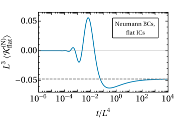
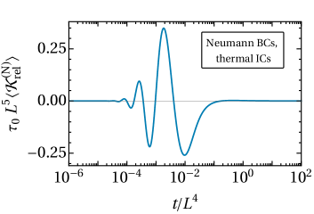
Figure 7: Time evolution of the dynamic CCF $\langle\mathcal{K}^{\text{(N)}}(t)\rangle$ [per $k_{B}T_{c}$, Eq. 109] in a thin film for Neumann BCs and $d=3$ dimensions. At time $t=0$, the system is instantaneously quenched to the bulk critical temperature ($\tau=0$). Panel (a) shows the CCF for flat ICs and the dashed line indicates the value of the equilibrium CCF at $T_{c}$ [Eq. 110]. Panel (b) shows the contribution $\tau_{0}\langle\mathcal{K}^{\text{(N)}}_{\text{rel}}(t)\rangle$ to the CCF $\langle\mathcal{K}^{\text{(N)}}_{\text{th}}(t)\rangle=\langle\mathcal{K}^{\text{(N)}}_{\text{flat}}(t)\rangle+\langle\mathcal{K}^{\text{(N)}}_{\text{rel}}(t)\rangle$ for thermal ICs [see Eq. 1], where $\tau_{0}=1/v$ is a measure of the initial temperature [see Eq. 48]. In both panels, CCF and time are scaled according to Eq. 13, such that the universal behavior of the CCF scaling function is exhibited by the plot explicitly.

V.3 Cubical box with periodic BCs

In the case of a finite cuboidal system with periodic BCs at all surfaces, the film pressure follows from Eq. 92 [analogously to Eq. 95] as

$$\langle\mathcal{P}_{f}^{\text{(p)}}(t)\rangle=\frac{3}{2}\langle\mathcal{R}^{\text{(p)}}(t)\rangle-\frac{1}{2}\langle\mathcal{Q}^{\text{(p)}}(t)\rangle,$$ (111)

with the correlators

$$\langle\mathcal{R}^{\text{(p)}}(t)\rangle \equiv\langle\partial_{z}\phi(\mathbf{0}_{\parallel},z,t)\partial_{z}\phi(\mathbf{0}_{\parallel},z,t)\rangle\big{|}_{z\in\{0,L\}}=\frac{1}{AL}\sum_{\mathbf{p},n}(\lambda_{n}^{\text{(p)}})^{2}\langle|a_{n}(\mathbf{p},t)|^{2}\rangle=-\langle\phi(\mathbf{0}_{\parallel},z,t)\partial_{z}^{2}\phi(\mathbf{0}_{\parallel},z,t)\rangle\big{|}_{z\in\{0,L\}}$$

$$=-\partial_{z}^{2}\mathcal{C}^{\text{(p)}}(\mathbf{0}_{\parallel},z,t)\big{|}_{z\in\{0,L\}}=-\sum_{\{m_{\alpha}=-\infty\}}^{\{\infty\}}\partial_{z}^{2}\mathcal{C}_{b}(r,t)\big{|}_{\mathbf{r}=\bm{\mathcal{L}}(\mathbf{m})}\,,$$ (112a)

$$\langle\mathcal{Q}^{\text{(p)}}(t)\rangle \equiv\Big{\langle}\phi(\mathbf{r}_{\parallel},z,t)\nabla_{\parallel}^{2}\phi(\mathbf{r}_{\parallel},z,t)\Big{\rangle}\Big{|}_{{\mathbf{r}_{\parallel}=\mathbf{0}}\atop{z\in\{0,L\}}}=-\frac{1}{AL}\sum_{\mathbf{p},n}\mathbf{p}^{2}\langle|a_{n}(\mathbf{p},t)|^{2}\rangle=-\sum_{\alpha=1}^{d-1}\langle(\partial_{\alpha}\phi(\mathbf{r}_{\parallel},z,r))^{2}\rangle\Big{|}_{{\mathbf{r}_{\parallel}=\mathbf{0}_{\parallel}}\atop{z\in\{0,L\}}}$$

$$=\nabla_{\parallel}^{2}\mathcal{C}^{\text{(p)}}(\mathbf{r}_{\parallel},z,t)\big{|}_{{\mathbf{r}_{\parallel}=\mathbf{0}_{\parallel}}\atop{z\in\{0,L\}}}=\sum_{\{m_{\alpha}=-\infty\}}^{\{\infty\}}\nabla_{\parallel}^{2}\mathcal{C}_{b}(r,t)\big{|}_{\mathbf{r}=\bm{\mathcal{L}}(\mathbf{m})},$$ (112b)

where we have applied the Poisson resummation formula via Eq. 75. [For further details regarding the notation, see Eqs. 72 and 74.] With the aid of Eq. 97, the required derivatives are obtained as

$$\partial_{z}^{2}\mathcal{C}_{b}(r,t) =\left(\frac{1}{r}-\frac{z^{2}}{r^{3}}\right)\partial_{r}\mathcal{C}_{b}+\frac{z^{2}}{r^{2}}\partial_{r}^{2}\mathcal{C}_{b}(r,t),$$ (113a)

$$\nabla_{\parallel}^{2}\mathcal{C}_{b} =\left(\frac{d-2}{r}+\frac{z^{2}}{r^{3}}\right)\partial_{r}\mathcal{C}_{b}+\left(1-\frac{z^{2}}{r^{2}}\right)\partial_{r}^{2}\mathcal{C}_{b}.$$ (113b)

In the Poisson representation in Eq. 112, the terms pertaining to $\mathbf{m}=\mathbf{0}$ (i.e., $m_{1}=\ldots=m_{d}=0$) provide the bulk contribution to the CCF. Accordingly, defining the indicator function

$$\Theta(\mathbf{m})\equiv\begin{cases}0\quad&\text{if }\mathbf{m}=\mathbf{0},\\ 1&\text{otherwise,}\end{cases}$$ (114)

the CCF follows from Eq. 111 as

$$\langle\mathcal{K}^{\text{(p)}}(t)\rangle=-\sum_{m_{1}=-\infty}^{\infty}\cdots\sum_{m_{d}=-\infty}^{\infty}\Theta(\mathbf{m})\left[\left(\frac{1}{2}+\frac{z^{2}}{r^{2}}\right)\partial_{r}^{2}\mathcal{C}_{b}+\left(\frac{1+d}{2r}-\frac{z^{2}}{r^{3}}\right)\partial_{r}\mathcal{C}_{b}\right]_{\mathbf{r}=\bm{\mathcal{L}}(\mathbf{m})}.$$ (115)

V.3.1 Equilibrium CCF

We now demonstrate that Eq. 115 leads to the canonical equilibrium CCF which has previously been obtained in Ref. Gross et al. (2017) based on statistical field theory. We emphasize that evaluating Eq. 115 with the correlation function obtained at bulk criticality $\tau=0$, i.e., $\mathcal{C}_{b}=\mathcal{S}_{\text{stat}}$ [see Eq. 59], does not result in the correct equilibrium CCF at $\tau=0$ (see Appendix D). Instead, for the purpose of regularizating the zero-mode divergence [see the discussion following Eq. 79] it is necessary to consider a nonzero $\tau$ and perform the limit $\tau\to 0$ only at the end of the calculation. For nonzero $\tau$, Eq. 91 renders, analogously to Eq. 111, the canonical equilibrium film pressure

$$\begin{split}\langle\mathcal{P}_{f}^{\text{(p)}}\rangle_{\text{eq}}&=\frac{3}{2}\langle\mathcal{R}^{\text{(p)}}\rangle_{\text{eq}}-\frac{1}{2}\langle\mathcal{Q}^{\text{(p)}}\rangle_{\text{eq}}+\frac{1}{2}\tau\mathcal{C}^{\text{(p)}}_{\text{eq}}(\mathbf{r}_{\parallel}=\mathbf{0}_{\parallel},z=0),\\ &=\frac{3}{2}\langle\mathcal{R}^{\text{(p)}}\rangle_{\text{eq}}-\frac{1}{2}\langle\mathcal{Q}^{\text{(p)}}\rangle_{\text{eq}}+\frac{1}{2}\tau\mathcal{C}^{\text{(p)}}_{\text{eq,gc}}(\mathbf{r}_{\parallel}=\mathbf{0}_{\parallel},z=0)-\frac{1}{2}L^{-d}\varrho^{d-1},\end{split}$$ (116)

where we have used Eq. 79 in order to replace the canonical by the grand canonical static correlation function (for $\Phi=0$). In order to reformulate Eq. 116, we invoke the Schwinger-Dyson equation (see, e.g., Refs. Le Bellac (1991); Dean and Gopinathan (2010)),

$$\left\langle\phi(\mathbf{r})\frac{\delta\mathcal{F}}{\delta\phi(\mathbf{r}^{\prime})}\right\rangle=\delta(\mathbf{r}-\mathbf{r}^{\prime}),$$ (117)

which, in the Gaussian case and for $\tau\neq 0$, implies the following identity for the static bulk correlation function (see also Ref. Mikheev and Weeks (1991)):

$$-\nabla^{2}\mathcal{C}_{\text{b,eq}}(\mathbf{r})+\tau\mathcal{C}_{\text{b,eq}}(\mathbf{r})=\delta(\mathbf{r}).$$ (118)

Inserting this relation into Eq. 112b, with $\nabla^{2}=\nabla_{\parallel}^{2}+\partial_{z}^{2}$, renders

$$\langle\mathcal{Q}^{\text{(p)}}\rangle_{\text{eq}}=\langle\mathcal{R}^{\text{(p)}}\rangle_{\text{eq}}+\tau\underbrace{\sum_{\{m_{\alpha}=-\infty\}}^{\{\infty\}}\mathcal{C}_{\text{b,eq}}(\bm{\mathcal{L}}(\mathbf{m}))}_{\mathcal{C}^{\text{(p)}}_{\text{eq,gc}}(\mathbf{0}_{\parallel},0)}-\delta(\mathbf{0}),$$ (119)

where we have used Eqs. 75 and 80 in order to identify the static finite-size correlation function $\mathcal{C}^{\text{(p)}}_{\text{eq,gc}}$ (which pertains to the grand canonical ensemble). Accordingly, we obtain from Eq. 116 the canonical equilibrium film pressure

$$\langle\mathcal{P}_{f}^{\text{(p)}}\rangle_{\text{eq}}=\langle\mathcal{R}^{\text{(p)}}\rangle_{\text{eq}}-\frac{1}{2}\delta(\mathbf{0})-\frac{1}{2}L^{-d}\varrho^{d-1}.$$ (120)

The singular term $\delta(\mathbf{0})$ acquires a well-defined meaning by regularizing the theory on a lattice. Specifically, upon expressing Eq. 118 in Fourier space, one obtains the regularized form $\delta(0)=\int_{-\pi/\ell}^{\pi/\ell}\mathrm{d}k/(2\pi)=1/\ell$, where $\ell$ denotes the lattice constant. However, since $\delta(\mathbf{0})$ is actually independent of $L$ (and therefore represents a bulk term irrelevant for the CCF), it is not necessary to actually perform this regularization here. The last term on the r.h.s. of Eq. 120 stems from the absence of the zero-mode fluctuations [see Eq. 5] in the canonical ensemble Gross et al. (2017). Its specific form is closely related to the contribution $\mu\phi$ in the dynamical stress tensor [Eq. 86], such that, without it, one would obtain the wrong sign for the last term in Eq. 120. The zero-mode contribution $L^{-d}\varrho^{d-1}/2$ in Eq. 79 plays no role for the correlators $\langle\mathcal{R}^{\text{(p)}}\rangle_{\text{eq}}$ and $\langle\mathcal{Q}^{\text{(p)}}\rangle_{\text{eq}}$, because they are derivatives of the correlation function. Hence, they take the same form in the canonical and the grand canonical ensemble. Furthermore, in the thin film limit $\varrho\to 0$, Eq. 120 implies that $\langle\mathcal{P}_{f}\rangle_{\text{eq}}=\langle\mathcal{P}_{f}\rangle_{\text{eq,gc}}$ and hence

$$\langle\mathcal{K}^{\text{(p)}}\rangle_{\text{eq}}=\langle\mathcal{K}^{\text{(p)}}\rangle_{\text{eq,gc}},\qquad(\text{thin film},\varrho\to 0),$$ (121)

consistent with Eq. 100.

One is left with determining the expression of $\langle\mathcal{R}^{\text{(p)}}\rangle_{\text{eq}}$ in Eq. 120 for arbitrary $\tau\geq 0$. Inserting Eq. 45 into the first line of Eq. 112a, one obtains

$$\begin{split}\langle\mathcal{R}^{\text{(p)}}\rangle_{\text{eq}}&=\frac{1}{AL}\sum_{\mathbf{n_{\parallel}},n_{d}}\frac{(\lambda_{n_{d}}^{\text{(p)}})^{2}}{(\lambda_{n_{d}}^{\text{(p)}})^{2}+\mathbf{p}_{\mathbf{n_{\parallel}}}^{2}+\tau}=\frac{1}{AL}\sum_{\mathbf{n_{\parallel}},n_{d}}(\lambda_{n_{d}}^{\text{(p)}})^{2}\int_{0}^{\infty}\mathrm{d}s\,e^{-s\left[(\lambda_{n_{d}}^{\text{(p)}})^{2}+\mathbf{p}_{\mathbf{n_{\parallel}}}^{2}+\tau\right]}\\ &=\frac{1}{2A}\frac{\mathrm{d}}{\mathrm{d}L}\sum_{\mathbf{n_{\parallel}},n_{d}}\int_{0}^{\infty}\frac{\mathrm{d}s}{s}\exp\left\{-s\left[\tau+\left(\frac{2\pi n_{d}}{L}\right)^{2}+\sum_{\alpha=1}^{d-1}\left(\frac{2\pi n_{\alpha}}{L_{\parallel}}\right)^{2}\right]\right\}\\ &=\frac{1}{2A}\frac{\mathrm{d}}{\mathrm{d}L}\sum_{\mathbf{n_{\parallel}},n_{d}}\int_{0}^{\infty}\frac{\mathrm{d}s}{s}\exp\left\{-s\left[\frac{L^{2}\tau}{4\pi^{2}}+n_{d}^{2}+\varrho^{2}\sum_{\alpha=1}^{d-1}n_{\alpha}^{2}\right]\right\}\\ &=\frac{1}{2A}\frac{\mathrm{d}}{\mathrm{d}L}\int_{0}^{\infty}\frac{\mathrm{d}s}{s}\,\exp\left(-\frac{L^{2}\tau s}{4\pi^{2}}\right)\vartheta(s)[\vartheta(\varrho^{2}s)]^{d-1},\end{split}$$ (122)

where

$$\vartheta(y)=\sum_{n=-\infty}^{\infty}e^{-yn^{2}}$$ (123)

is the Jacobi theta function Olver et al. (2010). Note that the total derivative $\mathrm{d}/\mathrm{d}L$ also acts on $\varrho$, which is a function of $L$ [see Eq. 4]. The corresponding bulk contribution follows from Eq. 122 by replacing the sum over the eigenspectrum $\mathbf{n}$ by integrals according to Eq. 81, which essentially amounts to replacing $\vartheta(y)$ in Eq. 122 with $\int_{-\infty}^{\infty}\mathrm{d}n\,e^{-yn^{2}}=(\pi/y)^{1/2}$ . After subtraction of all bulk contributions, the canonical equilibrium CCF for $\tau\geq 0$ follows from Eq. 120 as

$$\begin{split}\langle\mathcal{K}^{\text{(p)}}\rangle_{\text{eq}}&=-\frac{1}{2A}\frac{\mathrm{d}}{\mathrm{d}L}\int_{0}^{\infty}\frac{\mathrm{d}s}{s}\exp\left(-\frac{L^{2}\tau s}{4\pi^{2}}\right)\left\{\varrho^{-d+1}\left(\frac{\pi}{s}\right)^{d/2}-\vartheta(s)[\vartheta(\varrho^{2}s)]^{d-1}\right\}-\frac{1}{2}L^{-d}\varrho^{d-1}\\ &=\langle\mathcal{K}^{\text{(p)}}\rangle_{\text{eq,gc}}-\frac{1}{2}L^{-d}\varrho^{d-1}.\end{split}$$ (124)

Here, we have used Eq. 4, which implies

$$\frac{1}{AL}=L^{-d}\varrho^{d-1},$$ (125)

and have identified the grand canonical CCF as

$$\langle\mathcal{K}^{\text{(p)}}\rangle_{\text{eq,gc}}=-\frac{\mathrm{d}}{\mathrm{d}L}\left[\frac{1}{2}L^{-d+1}\int_{0}^{\infty}\frac{\mathrm{d}s}{s}\exp\left(-\frac{L^{2}\tau s}{4\pi^{2}}\right)\left\{\left(\frac{\pi}{s}\right)^{d/2}-\vartheta(s)[\varrho\vartheta(\varrho^{2}s)]^{d-1}\right\}\right].$$ (126)

The expression in Eq. 124 fulfills the scaling form given in Eq. 13 (with $v=0$; see Ref. Gross et al. (2017)).

Notably, Eq. 122 can be written as $\langle\mathcal{R}^{\text{(p)}}\rangle_{\text{eq}}=-\mathrm{d}\mathcal{F}^{\text{(p)}}_{\text{gc}}/\mathrm{d}L$, where $\mathcal{F}^{\text{(p)}}_{\text{gc}}=(1/2)\sum_{\mathbf{n}_{\parallel},n_{d}}\ln(\mathbf{p}_{\mathbf{n}_{\parallel}}^{2}+(\lambda_{n_{d}}^{\text{(p)}})^{2})$ is the (unregularized) grand canonical free energy of the system (for $\Phi=0$) . The expression in the square brackets in Eq. 126 thus represents the associated grand canonical residual finite-size free energy per area, $\mathcal{F}_{\text{res}}/A$ Gross et al. (2017); Dohm (2011) . These results demonstrate that the stress tensor formalism used here leads to the same expression for the equilibrium CCF as the approach based on the free energy.

The limit $\tau\to 0$ of Eq. 126 is singular, and must be performed after computing the integral and the derivative (see Appendix E for further discussions). The canonical equilibrium CCF obtained from Eq. 124 at bulk criticality, i.e., $\tau\to 0$, is shown in Fig. 8 as a function of the aspect ratio $\varrho$. An asymptotic analysis (see Appendix E) reveals that, for a cubic geometry ($\varrho=1$) and at bulk criticality, the grand canonical CCF attains the remarkably simple value

$$\langle\mathcal{K}^{\text{(p)}}\rangle_{\text{eq,gc}}\big{|}_{\tau\to 0,\varrho=1}\simeq-\frac{1}{L^{d}}\frac{1}{d}.$$ (127)

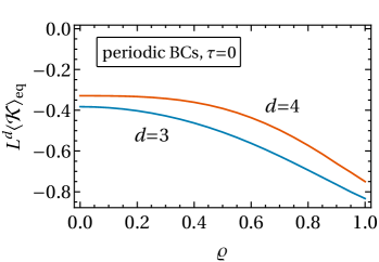
Figure 8: Canonical CCF in thermal equilibrium [Eq. 124] for a box with periodic BCs in all directions at bulk criticality ($\tau=0$) as a function of the aspect ratio $\varrho$, for $d=3$ and $d=4$ dimensions. $\mathcal{K}$ is taken in units of $k_{B}T_{c}$ so that it has the units of an inverse volume.

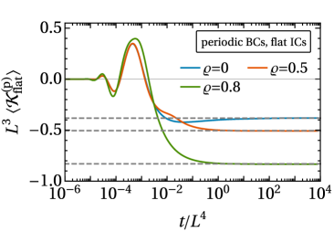
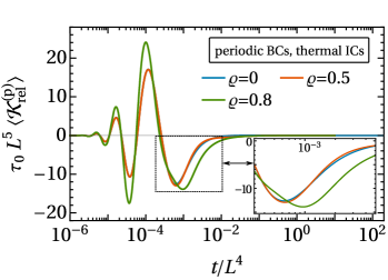
Figure 9: Time evolution of the dynamic CCF $\langle\mathcal{K}^{\text{(p)}}(t)\rangle$ [in $d=3$ and per $k_{B}T_{c}$, Eq. 115] for a box with periodic BCs for various aspect ratios $\varrho$ ($\varrho=0$ is the thin film limit). At time $t=0$, the system is instantaneously quenched to the bulk critical temperature ($\tau=0$). Panel (a) shows the CCF for flat ICs. The dashed lines indicate the equilibrium CCF at $T_{c}$ [see Eq. 124 and Fig. 8]. Panel (b) shows the contribution $\tau_{0}\langle\mathcal{K}^{\text{(p)}}_{\text{rel}}(t)\rangle$ (see Subsec. V.3.3) to the CCF for thermal ICs [see Eq. 1], where $\tau_{0}=1/v$ is a measure for the initial temperature [see Eq. 48]. In both panels, the CCF and the time are scaled according to Eq. 13, such that the universal behavior of the CCF scaling function is exhibited in the plot.

V.3.2 Dynamic CCF for flat ICs

The time-dependent CCF $\langle\mathcal{K}_{\text{flat}}^{\text{(p)}}(t)\rangle$ for flat ICs is obtained by evaluating Eq. 115 using Eq. 64, i.e., $\mathcal{C}_{b}(r,t)=\mathcal{S}_{\text{flat}}(r,t)=\mathcal{S}_{\text{stat}}(r)-\mathcal{S}_{\text{dyn}}(r,t)$. According to Eq. 65, $\mathcal{S}_{\text{flat}}$ vanishes exponentially in the limit $t\to 0$, which implies

$$\langle\mathcal{K}_{\text{flat}}^{\text{(p)}}(t=0)\rangle=0.$$ (128)

At late times $t\gg L{z}$ (which corresponds to ${\tilde{t}}/\mathpzc{\tilde{t}}_{+}^{(0)}\gg(L/\xi_{+}^{(0)})^{z}$, $z=4$), $\langle\mathcal{K}_{\text{flat}}^{\text{(p)}}(t)\rangle$ approaches the equilibrium value of the CCF given in Eq. 124. Obtaining this result from the dynamics is, however, intricate because not only $\mathcal{S}_{\text{stat}}$, but also $\mathcal{S}_{\text{dyn}}$ contributes to the late-time limit of $\langle\mathcal{K}_{\text{flat}}^{\text{(p)}}(t)\rangle$, despite the fact that $\mathcal{S}_{\text{dyn}}(r,t)$ and its derivatives vanish algebraically for large $t$ [see Eq. 60]:

$$\partial_{r}^{2}\mathcal{S}_{\text{dyn}}(r,t\to\infty)\sim\frac{1}{r}\partial_{r}\mathcal{S}_{\text{dyn}}(r,t\to\infty)\sim-t^{-d/4}.$$ (129)

The reason for the nonzero contribution of $\mathcal{S}_{\text{dyn}}$ to $\langle\mathcal{K}^{\text{(p)}}_{\text{flat}}(t\gg L{z})\rangle$ is the $d$-fold summation in Eq. 115, which, as shown in Appendix F, balances the rather mild algebraic decay in Eq. 129 . The summation in Eq. 115 therefore does not commute with the limit $t\to\infty$.

The contribution to the equilibrium CCF stemming from $\mathcal{S}_{\text{dyn}}$ can be calculated exactly in $d=1$ spatial dimensions (see Appendix F), while it has to be determined numerically for $d>1$. The universal behavior of $\langle\mathcal{K}^{\text{(p)}}_{\text{flat}}(t)\rangle$ is illustrated in Fig. 9(a) as a function of time for $d=3$ and various aspect ratios $\varrho$. For an accurate estimate it suffices to take into account only terms with $|m_{1,\ldots,d}|\lesssim\mathcal{O}(100)$ in the numerical evaluation of Eq. 115, the precise number for truncation depending somewhat on the value of $t/L^{z}$ being considered. The computation can be further sped up by exploiting the isotropy of the expression in the lateral directions. Notably, for $\varrho=1$, the contribution to $\langle\mathcal{K}_{\text{flat}}^{\text{(p)}}(t)\rangle$ stemming from $\mathcal{S}_{\text{stat}}$ vanishes identically (see Appendix D), implying, in particular, that the equilibrium value $\langle\mathcal{K}_{\text{flat}}^{\text{(p)}}\rangle_{\text{eq}}<0$ (see Fig. 8) arises within the dynamics solely due to $\mathcal{S}_{\text{dyn}}$. In Fig. 9 one observes that changing the aspect ratio mainly affects the late-time equilibrium value of the CCF.

V.3.3 Dynamic CCF for thermal ICs

Analogously to Eq. 104, the dynamic CCF $\langle\mathcal{K}^{\text{(p)}}_{\text{th}}(t)\rangle$ for thermal ICs, obtained by inserting Eq. 70 into Eq. 115, can be split up into the contributions $\langle\mathcal{K}^{\text{(p)}}_{\text{flat}}(t)\rangle$ and $\langle\mathcal{K}^{\text{(p)}}_{\text{rel}}(t)\rangle$. In contrast to $\langle\mathcal{K}^{\text{(p)}}_{\text{flat}}(t)\rangle$ discussed in the preceding subsection, $\langle\mathcal{K}^{\text{(p)}}_{\text{rel}}(t)\rangle$ does not contribute to the late-time limit of the CCF, because according to Eq. 62 the relevant derivatives of $\mathcal{S}_{\text{rel}}$ decay more rapidly than those in Eq. 129:

$$\partial_{r}^{2}\mathcal{S}_{\text{rel}}(r,t\to\infty)\sim\frac{1}{r}\partial_{r}\mathcal{S}_{\text{dyn}}(r,t\to\infty)\sim-t^{-(d+2)/4}.$$ (130)

Instead, $\langle\mathcal{K}^{\text{(p)}}_{\text{rel}}(t)\rangle$, which is illustrated in Fig. 9(b), contributes to $\langle\mathcal{K}^{\text{(p)}}_{\text{th}}(t)\rangle$ only at intermediate times with a magnitude $\propto 1/\tau_{0}$ [see Eq. 1].

V.4 Cubical box with Neumann BCs

The calculation of the CCF for Neumann BCs in a cuboidal box proceeds analogously to Secs. V.2 and V.3. Therefore we summarize here only the main steps. In the box geometry, the film pressure is given by the same expression as for the thin film [Eq. 107], i.e.,

$$\langle\mathcal{P}_{f}^{\text{(N)}}(t)\rangle=\langle\mathcal{R}^{\text{(N)}}(t)\rangle-\frac{1}{2}\langle\mathcal{Q}^{\text{(N)}}(t)\rangle,$$ (131)

but with [see Eq. 74 for the notation]

$$\langle\mathcal{R}^{\text{(N)}}(t)\rangle =-2\sum_{\{m_{\alpha}=-\infty\}}^{\{\infty\}}\partial_{z}^{2}\mathcal{C}_{b}(\{\mathbf{r}_{\parallel},z\},t)\big{|}_{\mathbf{r}=\tilde{\bm{\mathcal{L}}}(\mathbf{m})}=2\langle\mathcal{R}^{\text{(p)}}(t)\rangle\big{|}_{2L}\,,$$ (132a)

$$\langle\mathcal{Q}^{\text{(N)}}(t)\rangle =2\sum_{\{m_{\alpha}=-\infty\}}^{\{\infty\}}\nabla^{2}_{\parallel}\mathcal{C}_{b}(\{\mathbf{r}_{\parallel},z\},t)\big{|}_{\mathbf{r}=\tilde{\bm{\mathcal{L}}}(\mathbf{m})}=2\langle\mathcal{Q}^{\text{(p)}}(t)\rangle\big{|}_{2L}\,,$$ (132b)

where $\langle\mathcal{R}^{\text{(p)}}\rangle$ and $\langle\mathcal{Q}^{\text{(p)}}\rangle$ refer to the expressions for a box with periodic BCs given in Eq. 112, which are to be evaluated here for the film thickness $2L$. Using Eq. 113, the CCF follows from Eq. 131 as

$$\langle\mathcal{K}^{\text{(N)}}(t)\rangle=-\sum_{m_{x}=-\infty}^{\infty}\cdots\sum_{m_{z}=-\infty}^{\infty}\Theta(\mathbf{m})\left[\left(1+\frac{z^{2}}{r^{2}}\right)\partial_{r}^{2}\mathcal{C}_{b}+\left(\frac{d}{r}-\frac{z^{2}}{r^{3}}\right)\partial_{r}\mathcal{C}_{b}\right]_{\mathbf{r}=\tilde{\bm{\mathcal{L}}}(\mathbf{m})},$$ (133)

where, analogously to Eq. 115, the term pertaining to $\mathbf{m}=\mathbf{0}$ [see Eq. 114] is identified with the bulk pressure and is therefore absent in the sum.

V.4.1 Equilibrium CCF

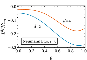
Figure 10: Canonical CCF in thermal equilibrium [Eq. 124] for a box with Neumann BCs in the transverse direction and periodic BCs in the lateral directions at bulk criticality ($\tau=0$) as a function of the aspect ratio $\varrho$, for $d=3$ and $d=4$ dimensions. $\mathcal{K}$ is taken in units of $k_{B}T_{c}$ so that it has the units of an inverse volume.

In order to obtain the equilibrium CCF, we proceed as in Sec. V.3.1 and consider Eq. 91 in equilibrium for arbitrary $\tau\geq 0$. This renders the film pressure

$$\begin{split}\langle\mathcal{P}_{f}^{\text{(N)}}\rangle_{\text{eq}}&=\langle\mathcal{R}^{\text{(N)}}\rangle_{\text{eq}}-\frac{1}{2}\langle\mathcal{Q}^{\text{(N)}}\rangle_{\text{eq}}+\frac{1}{2}\tau\mathcal{C}^{\text{(N)}}_{\text{eq}}(\mathbf{0}_{\parallel},z\in\{0,L\})\\ &=\langle\mathcal{R}^{\text{(N)}}\rangle_{\text{eq}}-\frac{1}{2}\langle\mathcal{Q}^{\text{(N)}}\rangle_{\text{eq}}+\frac{1}{2}\tau\mathcal{C}^{\text{(N)}}_{\text{eq,gc}}(\mathbf{0}_{\parallel},z\in\{0,L\})-\frac{1}{2}L^{-d}\varrho^{d-1},\end{split}$$ (134)

where we have used Eq. 79. Since the relations between periodic and Neumann BCs provided by Eq. 132 hold also in the equilibrium case, the analogous form of Eq. 119 for Neumann BCs follows by using Eqs. 78, 132, and 119 as $\langle\mathcal{Q}^{\text{(N)}}\rangle_{\text{eq}}=\langle\mathcal{R}^{\text{(N)}}\rangle_{\text{eq}}+\tau\mathcal{C}^{\text{(N)}}_{\text{eq,gc}}(\mathbf{0}_{\parallel},z\in\{0,L\})-2\delta(\mathbf{0})$. Inserting this into Eq. 134 renders

$$\langle\mathcal{P}_{f}^{\text{(N)}}\rangle_{\text{eq}}=\frac{1}{2}\langle\mathcal{R}^{\text{(N)}}\rangle_{\text{eq}}+\delta(\mathbf{0})-\frac{1}{2}L^{-d}\varrho^{d-1}.$$ (135)

The quantity $\delta(\mathbf{0})$ is defined as in Eq. 120 and represents a bulk contribution, while the term $-L^{-d}\varrho^{-d}/2$ is due to the global OP conservation. The equilibrium CCF for a box with Neumann BCs follows from Eq. 135 as

$$\langle\mathcal{K}^{\text{(N)}}(\tau,\varrho,L)\rangle_{\text{eq}}=\langle\mathcal{K}^{\text{(N)}}(\tau,\varrho,L)\rangle_{\text{eq,gc}}-\frac{1}{2}L^{-d}\varrho^{d-1},$$ (136)

where, using Eqs. 120 and 132a, the grand canonical CCF $\langle\mathcal{K}^{\text{(N)}}\rangle_{\text{eq,gc}}$ can be expressed in terms of the corresponding one for periodic BCs [Eq. 126] as

$$\langle\mathcal{K}^{\text{(N)}}(\tau,\varrho,L)\rangle_{\text{eq,gc}}=\langle\mathcal{K}^{\text{(p)}}(\tau,2\varrho,2L)\rangle_{\text{eq,gc}}=2^{-d}\langle\mathcal{K}^{\text{(p)}}(4\tau,2\varrho,L)\rangle_{\text{eq,gc}}.$$ (137)

In the last relation, we have used the fact that $\tau$ enters the underlying expression only in the combination $L^{2}\tau$. The CCF in Eq. 136 fulfils the scaling form given in Eq. 13 (with $v=0$) Gross et al. (2017) and is illustrated in Fig. 10 at bulk criticality, i.e., $\tau\to 0$, as a function of $\varrho$.

V.4.2 Dynamic CCF

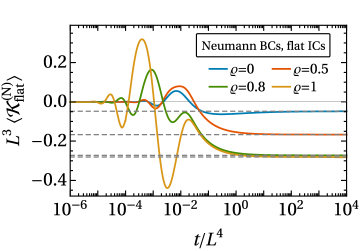
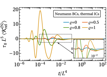
Figure 11: Time evolution of the dynamic CCF [in $d=3$ and per $k_{B}T_{c}$, Eq. 133] for a box with Neumann BCs in the transverse direction (and periodic BCs in the lateral directions) for various aspect ratios $\varrho$ ($\varrho=0$ is the thin film limit). At time $t=0$, the system is instantaneously quenched to the bulk critical temperature ($\tau=0$). Panel (a) shows the CCF for flat ICs. The dashed lines indicate the equilibrium CCF at $T_{c}$ [see Eq. 136 and Fig. 10]. Panel (b) shows the contribution $\tau_{0}\langle\mathcal{K}^{\text{(N)}}_{\text{rel}}(t)\rangle$ [see Subsec. V.4.2] to the CCF for thermal ICs [see Eq. 1], where $\tau_{0}=1/v$ is a measure of the initial temperature [see Eq. 48]. In both panels, CCF and time are scaled according to Eq. 13, such that the universal behavior of the CCF scaling function is exhibited in the plot.

The time-dependent CCF for flat and thermal ICs follows from Eq. 133 upon inserting Eq. (64) or (70) for the bulk correlation function $\mathcal{C}_{b}$. Analogously to the case of periodic BCs (see Sec. V.3.2), at late times $t\gg L^{z}$, the dynamic CCF receives contributions both from the static and the dynamic correlators, $\mathcal{S}_{\text{stat}}$ and $\mathcal{S}_{\text{dyn}}$. Accordingly, in Eq. 133 the limit $t\to\infty$ must be performed after the summation in order to obtain the correct equilibrium value [Eq. 136] of the CCF.

As illustrated in Fig. 11(a), the dynamic CCF for Neumann BCs and flat ICs initially vanishes and approaches its late-time, equilibrium value [see Eqs. 136 and 10] in a non-monotonous fashion. Figure 11(b) shows the contribution $\langle\mathcal{K}_{\text{rel}}^{\text{(N)}}(t)\rangle$ to the CCF for thermal ICs, which is obtained by inserting $\mathcal{C}_{b}=\mathcal{S}_{\text{rel}}$ [Eq. 61] into Eq. 133 [see also Eq. 104]. In contrast to the case of periodic BCs [see Fig. 9], increasing the aspect ratio $\varrho$ from 0 to 1 has a pronounced effect on the time-dependent CCF, inducing, in particular, a shift of the location of the major maximum of the CCF towards shorter times. A heuristic understanding of this behavior can be gained by noting that, according to Eq. 9, the term in the square brackets in Eq. 133 has the scaling form $r^{-d}K(\psi)$, $\psi=r^{4}/(512t)=L^{4}(r_{\parallel}^{2}/(2\varrho)^{2}+z^{2})^{2}/t$, where the scaling function $K(\psi)$ attains its maximum for $\psi\sim\mathcal{O}(1)$ and vanishes for $\psi\to\infty$ with exponentially decaying oscillations [see Eqs. 63 and 65]. We note the factor 2 multiplying $\varrho$ in the expression for $\psi$, which stems from the fact that the expression in the square brackets in Eq. 133 has to be evaluated for $z=2m_{z}L$. Accordingly, in Eq. 133 for $\varrho\lesssim 1/2$, the transverse mode $\mathbf{m}=\{0,\ldots,0,1\}$ is dominant and the temporal shape of the CCF depends only weakly on $\varrho$. In contrast, for $\varrho\gtrsim 1/2$ and a lateral mode $\mathbf{m}\in\{\{1,0,\ldots,0\},\{0,1,0,\ldots,0\},\ldots\}$, one reaches $\psi\sim\mathcal{O}(1)$ already at small $t/L^{4}$. Thus these modes increasingly contribute to the CCF and are responsible for a shift of the maximum towards earlier times. The same reasoning applies also to the CCF for periodic BCs [see Fig. 9], except that here the crossover between the two regimes occurs for $\varrho\simeq 1$ (which is thus not apparent in the plots).

VI Summary and Outlook

We have studied the non-equilibrium dynamics of a confined fluid quenched to its critical point. The confinement is realized by a $d$-dimensional cuboid box of volume $V=LL_{\parallel}^{d-1}$, thickness $L$, and lateral size $L_{\parallel}$ (see Fig. 1). Included in this setup is the limit of a thin film, for which $L_{\parallel}\to\infty$. Our analysis is based on the (linearized) equations of model B, which describe a near-critical fluid with conserved OP, neglecting heat and momentum transport Hohenberg and Halperin (1977). In the case of a box, periodic or Neumann BCs are imposed in the transverse ($z$) direction and, for technical reasons, periodic BCs in the remaining, lateral directions. These BCs ensure that the total integrated OP $\Phi$ is conserved [see Eq. 5]. Accordingly, in equilibrium, which is achieved at late times ($t\to\infty$), the canonical ensemble is realized. We take the initial ($t=0$) OP to have a vanishing mean value and short-ranged correlations [see Eq. 1], amounting to a constant amplitude $\propto v$ of the initial OP variance (“thermal” initial conditions, ICs). This includes the case of a vanishing initial OP $\phi(\mathbf{r},t=0)=0$, which we call “flat” ICs [see Eq. 2]. Physically, thermal ICs correspond to starting the quench from equilibrium at a super-critical temperature which is sufficiently high to ensure a short initial correlation length.

Following Refs. Dean and Gopinathan (2010); Krüger et al. (2018); Gross et al. (2018), the present study focuses on the non-equilibrium critical Casimir force (CCF), which we define in terms of a generalized force acting on the confining boundaries of the system. The generalized force and the associated dynamical stress tensor Krüger et al. (2018); Gross et al. (2018) are determined by the finite-size OP correlation function and derivatives thereof, evaluated at coinciding spatial points.

Our main results can be summarized as follows:

1. We have presented analytical expressions for the static and dynamic correlation functions of an OP governed by model B at bulk criticality subject to periodic or Neumann BCs. These finite-size correlation functions are expressed, via the Poisson resummation formula, in terms of an infinite summation over “image points” of the bulk correlation function (see also Refs. Diehl and Dietrich (1981); Diehl and Ritschel (1993)). The latter is given in closed form in terms of generalized hypergeometric functions. In the Poisson representation of a finite-size quantity the bulk contribution can be explicitly identified, which facilitates the determination of the CCF.

2. The formalism, which is based on the recently introduced dynamic stress tensor Krüger et al. (2018); Gross et al. (2018), is shown to lead, in the late-time limit, to the same equilibrium CCF obtained previously within statistical field theory Krech and Dietrich (1992); Gross et al. (2017). In the case of a box geometry the total OP conservation gives rise to the canonical CCF Gross et al. (2017). In contrast, for a thin film the OP conservation is immaterial and the standard grand canonical CCF Krech and Dietrich (1992) is recovered. For periodic and Neumann BCs and a total OP $\Phi=0$, the value of the canonical CCF is (within the Gaussian approximation) reduced relative to the grand canonical one by the amount $1/(2V)$ [see Eqs. 124 and 136 and Ref. Gross et al. (2017)].

3. For all geometries and BCs considered here, the dynamic CCF vanishes initially. Physically, this can be understood as a consequence of the short-ranged correlations of the ICs [see Eq. 1] and the symmetry-preserving character of the BCs (i.e., there are no surface fields). The (non-zero) late-time, equilibrium value of the CCF is approached in an oscillatory growing fashion. This oscillatory behavior is in contrast to the more gentle growth of the dynamic CCF for quenches within model A dynamics (i.e., for non-conserved OP) in a critical film Dean and Gopinathan (2010), as well as to the purely transient, non-oscillatory forces reported for model B in systems far from criticality Rohwer et al. (2017, 2018).

4. Thermal ICs give rise to an additional transient at intermediate times, superimposed on the dynamics of the CCF pertaining to flat ICs. Thermal ICs do not affect the late-time behavior of the CCF. Their influence diminishes upon decreasing the amplitude of the initial OP correlations [see Eq. 1].

Within the framework of boundary critical phenomena Diehl (1986, 1997), imposing Neumann BCs for the OP [Eq. 25] at the Gaussian level corresponds to the so-called “special” surface universality class (SUC) . Besides the so-called “normal” SUC, the quench dynamics of which has been studied in Ref. Gross et al. (2018), another relevant SUC for fluids is the so-called “ordinary” SUC, corresponding (within the Gaussian approximation) to Dirichlet BCs. Each static SUC splits up into several dynamic SUCs depending on the dynamic model considered. In contrast to Neumann BCs, standard Dirichlet BCs do not entail a vanishing flux at the boundaries of the system. In fact, for semi-infinite geometries, in Refs. Diehl (1994); Wichmann and Diehl (1995) non-conservative dynamics at a surface has been shown to lead to a new dynamic SUC (called “model $\mathrm{B_{A}}$” in Ref. Diehl (1994)), which is distinct from the fully conservative model B Diehl and Janssen (1992) (denoted as “model $\mathrm{B_{B}}$” in this context). A modification of Dirichlet BCs in order to implement the no-flux condition is possible but leads to transcendental eigenvalues Gross (2018a, b) and is left for future investigations.

Another direction into which the present study can be extended, concerns the dynamics following a quench to a slightly super-critical temperature. In fact, in the high-temperature limit of model B, which in thermal equilibrium is free of long-ranged correlations, one observes a transient post-quench Casimir-like force induced solely by the dynamic conservation law Rohwer et al. (2017, 2018), while the equilibrium CCF vanishes.

It should also be rewarding to go beyond the Gaussian dynamics considered here, retaining the $\phi^{4}$ nonlinearity in the Landau-Ginzburg free energy functional. The nonlinear term is expected to lead, inter alia, to corrections of the early-time behavior after the quench Ritschel and Diehl (1996). Furthermore, the effect of a nonzero initial mean OP, i.e., $\langle\phi(\mathbf{r},t=0)\rangle=\Phi/V\neq 0$, could be investigated. In the case of non-conserved dynamics, it has been shown that a non-zero initial OP leads to a universal initial growth behavior of the OP, the so-called “critical initial slip” Janssen et al. (1989); Janssen (1992); Diehl and Ritschel (1993); Ritschel and Czerner (1995); Ritschel and Diehl (1996), which is described by a new dynamic critical exponent . Additionally, it would be insightful to explore the relationship between the present model and active matter systems in more detail Caballero et al. (2018).

Regarding the experimental realization of our findings, quenches of binary liquid mixtures to their critical demixing point appear to be promising candidates. Indeed, extending established experimental techniques for equilibrium CCFs (see, e.g., Ref. Hertlein et al. (2008)) to non-equilibrium scenarios is a timely issue. In this regard, the influence of thermal diffusion and momentum transport on the quench dynamics could be elucidated Oerding and Janssen (1993); Roy et al. (2018). Ultimately these studies should aim at the “normal” SUC as the one to which actual fluids belong due to the generic presence of symmetry breaking surface fields. Notably, while the “ordinary” SUC is experimentally realizable for fluids via a suitable tuning of the surface fields Desai et al. (1995); Nellen et al. (2009); Mohry et al. (2010), achieving conditions appropriate for the “special” SUC is still an open issue.

A more direct test of our predictions can be achieved via simulations, for which non-symmetry breaking BCs are easily realizable. Recently, progress has been made, e.g., within molecular dynamics Das et al. (2006); Roy et al. (2016) and within the lattice Boltzmann method Gross and Varnik (2012a, b); Belardinelli et al. (2015) towards simulation of critical dynamics and determining CCFs Puosi et al. (2016). Moreover, these simulation methods typically realize the canonical ensemble and thus allow one to test the ensemble differences of the CCF Gross et al. (2016, 2017).

Appendix A Poisson resummation formula

The Poisson resummation formula in its general form (see, e.g., Refs. Dohm (2008); Grüneberg and Diehl (2008); Diehl and Ritschel (1993)) states that, for a given function $\hat{f}(\mathbf{n})$ depending on $\mathbf{n}\in\mathbb{Z}^{D}$,

$$\sum_{\mathbf{n}}\hat{f}(\mathbf{n})=\sum_{\mathbf{m}}F(\mathbf{m}),$$ (138)

where $\mathbf{m}\in\mathbb{Z}^{D}$,

$$F(\mathbf{r})\equiv\int_{\mathbb{R}^{D}}\mathrm{d}^{D}k\,\hat{f}(\mathbf{k})e^{2\pi\mathrm{i}\mathbf{k}\cdot\mathbf{r}}=(2\pi)^{D}f(2\pi\mathbf{r}),$$ (139)

and

$$f(\mathbf{r})=\int_{\mathbb{R}^{D}}\frac{\mathrm{d}^{D}k}{(2\pi)^{D}}\,\hat{f}(\mathbf{k})e^{\mathrm{i}\mathbf{k}\cdot\mathbf{r}}$$ (140)

represents the standard ($D$-dimensional) inverse Fourier transform of $\hat{f}$.

Specifically, if $\hat{f}$ depends on a $D<d$ dimensional vector $\mathbf{n}\in\mathbb{Z}^{D}$ via the form $\hat{f}\left(\Big{\{}\frac{2\pi n_{\alpha}}{L_{\alpha}}\Big{\}}\right)$ with $L_{\alpha}\in\mathbb{R}$, $\alpha=1,\ldots,D$, Eq. 138 renders

$$\sum_{\mathbf{n}}\hat{f}\left(\Big{\{}\frac{2\pi n_{\alpha}}{L_{\alpha}}\Big{\}}\right)=\frac{\prod_{\alpha}L_{\alpha}}{(2\pi)^{D}}\sum_{\mathbf{m}}\int\mathrm{d}^{D}k\,\hat{f}(\mathbf{k})e^{\mathrm{i}k_{\alpha}m_{\alpha}L_{\alpha}}=\prod_{\alpha}L_{\alpha}\sum_{\mathbf{m}}f(\mathbf{r}=\bm{\mathcal{L}}(\mathbf{m})),$$ (141)

where $\bm{\mathcal{L}}(\mathbf{m})$ is a shorthand notation for the $D$-dimensional vector $\{m_{1}L_{1},\ldots,m_{D}L_{D}\}$ [see Eq. 74]. Another relevant case for the present study is obtained if $\hat{f}$ depends on $n=0,1,2,\ldots$ in the form $\hat{f}(n)=(2-\delta_{n,0})\hat{\vphantom{\rule{1.0pt}{5.71527pt}}\smash{\hat{f}}}\left(\frac{\pi|n|}{L}\right)$, with $L\in\mathbb{R}$ and some function $\hat{\vphantom{\rule{1.0pt}{5.71527pt}}\smash{\hat{f}}}$. Here, Eq. 138 renders

$$\begin{split}\sum_{n=0,1,\ldots}(2-\delta_{n,0})\hat{\vphantom{\rule{1.0pt}{5.71527pt}}\smash{\hat{f}}}\left(\frac{\pi|n|}{L}\right)&=2\sum_{n=0,1,\ldots}\hat{\vphantom{\rule{1.0pt}{5.71527pt}}\smash{\hat{f}}}\left(\frac{\pi|n|}{L}\right)-\hat{\vphantom{\rule{1.0pt}{5.71527pt}}\smash{\hat{f}}}(0)=\sum_{{n=-\infty,}\atop{n\neq 0}}^{\infty}\hat{\vphantom{\rule{1.0pt}{5.71527pt}}\smash{\hat{f}}}\left(\frac{\pi|n|}{L}\right)+\hat{\vphantom{\rule{1.0pt}{5.71527pt}}\smash{\hat{f}}}(0)\\ &=\sum_{n=-\infty}^{\infty}\hat{\vphantom{\rule{1.0pt}{5.71527pt}}\smash{\hat{f}}}\left(\frac{\pi|n|}{L}\right)=2L\sum_{m=-\infty}^{\infty}f(r=2Lm),\end{split}$$ (142)

where now, accordingly, $f$ in Eq. 140 is to be evaluated by replacing $\hat{f}$ by $\hat{\vphantom{\rule{1.0pt}{5.71527pt}}\smash{\hat{f}}}$ on the right-hand side.

Appendix B Static equilibrium correlation functions in a thin film

Here, we present analytic expressions for the static equilibrium correlation function $\mathcal{C}_{\text{eq}}(\mathbf{r}_{\parallel},z,z^{\prime})$ [Eq. 79] in a thin film for periodic as well as Neumann BCs. In this case, according to Eq. 83, $\mathcal{C}_{\text{eq}}$ is not affected by the choice of the ensemble.

B.1 Thin film with periodic BCs

Upon inserting $\mathcal{C}_{b}=\mathcal{S}_{\text{stat}}$ [Eq. 59] into Eq. 82a, the static correlation function for a thin film with periodic BCs follows as

$$\mathcal{C}^{\text{(p)}}_{\text{eq}}(r_{\parallel},z)=\frac{\Gamma(d/2-1)}{4\pi^{d/2}}\sum_{m=-\infty}^{\infty}\frac{1}{\left|(z+mL)^{2}+r_{\parallel}^{2}\right|^{d/2-1}}=\frac{\Gamma(d/2-1)}{4\pi^{d/2}L^{d-2}}\sum_{m=-\infty}^{\infty}\frac{1}{\left|(\zeta+m)^{2}+\hat{r}^{2}\right|^{d/2-1}},$$ (143)

where $\zeta\equiv z/L$ and $\hat{r}\equiv r_{\parallel}/L$. Due to the periodicity in the $z$-direction, $\mathcal{C}^{\text{(p)}}_{\text{eq}}$ depends only on one $z$ coordinate. For $r_{\parallel}\neq 0$, the sum represents an inhomogeneous Epstein zeta function which can be determined according to Eq. (4.13) in Ref. Elizalde (2012). This renders

$$\mathcal{C}^{\text{(p)}}_{\text{eq}}(r_{\parallel}>0,z)=\frac{1}{L^{d-2}}\Big{[}\frac{\Gamma(d/2-3/2)}{4\pi^{d/2-1/2}}\hat{r}^{3-d}+\frac{1}{\pi}\hat{r}^{(3-d)/2}\sum_{n=1}^{\infty}n^{d/2-3/2}\cos(2\pi n\zeta)K_{d/2-3/2}(2\pi n\hat{r})\Big{]},$$ (144)

with the modified Bessel function $K_{\nu}$ of the second kind. For $r_{\parallel}=0$, Eq. 143 can be expressed in terms of the Hurwitz zeta function $\zeta_{H}(s,q)$ Olver et al. (2010) as

$$\mathcal{C}^{\text{(p)}}_{\text{eq}}(r_{\parallel}=0,z)=\frac{\Gamma(d/2-1)}{4\pi^{d/2}L^{d-2}}\left[\frac{1}{\zeta^{d-2}}+\zeta_{H}(d-2,1+\zeta)+\zeta_{H}(d-2,1-\zeta)\right].$$ (145)

For $d\to 3$ one has $\zeta_{H}(d-2,u)\simeq\frac{1}{d-3}-\Psi(u)+\mathcal{O}(d-3)$, where $\Psi$ denotes the dilogarithm. The logarithmic divergence of the sum in Eq. 143 for $d=3$ is reflected by the simple poles $\sim 2/(d-3)$ in Eqs. 144 and 145, stemming from the contributions $\Gamma(d/2-3/2)$ and $\zeta_{H}$, respectively. Equations 143 and 144 are therefore valid for $d>3$. For $d=4$, the sum in Eq. 144 can be carried out in closed form, yielding

$$\mathcal{C}^{\text{(p)}}_{\text{eq}}(r_{\parallel},z)\big{|}_{d=4}=\frac{1}{4\pi Lr_{\parallel}}\Big{[}1+\frac{e^{-2\pi\hat{r}}-\cos(2\pi\zeta)}{\cos(2\pi\zeta)-\cosh(2\pi\hat{r})}\Big{]}.$$ (146)

For large lateral distances $\hat{r}\gg 1$, Eq. 146 reduces to $\mathcal{C}^{\text{(p)}}_{\text{eq}}(r_{\parallel}\gg L,z)\simeq(\pi/L)\mathcal{S}_{\text{stat}}(r_{\parallel})$, i.e., $\mathcal{C}^{\text{(p)}}_{\text{eq}}$ shows the same $r_{\parallel}$-dependence as the correlation function in a critical $d=3$ dimensional bulk system [Eq. 59]. On the other hand, in the limit $L\to\infty$ one obtains $\mathcal{C}^{\text{(p)}}_{\text{eq}}(r_{\parallel},z)\simeq 1/[4\pi^{2}(r_{\parallel}^{2}+z^{2})]$, i.e., the static bulk correlator [Eq. 59] for $d=4$.

B.2 Thin film with Neumann BCs

Upon using Eq. 144 and the last line of Eq. 77, the following form of the static equilibrium correlation function for a thin film with Neumann BCs is obtained:

$$\mathcal{C}^{\text{(N)}}_{\text{eq}}(r_{\parallel}>0,z,z^{\prime})=\frac{1}{L^{d-2}}\Bigg{[}\frac{\Gamma(d/2-3/2)}{4\pi^{d/2-1/2}}\hat{r}^{3-d}+\frac{1}{\pi}\hat{r}^{(3-d)/2}\sum_{n=1}^{\infty}\left(\frac{n}{2}\right)^{(d-3)/2}\cos(\pi n\zeta)\cos(\pi n\zeta^{\prime})K_{(d-3)/2}(\pi n\hat{r})\Bigg{]},$$ (147)

with $\zeta\equiv z/L$ and $\hat{r}\equiv r_{\parallel}/L$. In contrast to the periodic case, $\mathcal{C}^{\text{(N)}}_{\text{eq}}$ depends explicitly on $z^{\prime}$. For $z^{\prime}=0$, Eq. 147 differs from the periodic one [Eq. 144] only by the replacement $n\to n/2$ in the summation. For $r_{\parallel}=z^{\prime}=0$, one has

$$\mathcal{C}^{\text{(N)}}_{\text{eq}}(r_{\parallel}=0,z)=2^{3-d}\mathcal{C}^{\text{(p)}}_{\text{eq}}(r_{\parallel}=0,z/2).$$ (148)

In the case of $d=4$ dimensions, Eq. 147 can be determined explicitly, rendering [in analogy to Eq. 146]

$$\mathcal{C}^{\text{(N)}}_{\text{eq}}(r_{\parallel},z,z^{\prime})\big{|}_{d=4} =\frac{1}{8\pi Lr_{\parallel}}\frac{\sinh(\pi\hat{r})\big{[}\cos(\pi(\zeta-\zeta^{\prime}))+\cos(\pi(\zeta+\zeta^{\prime}))-2\cosh(\pi\hat{r})\big{]}}{\big{[}\cos(\pi(\zeta-\zeta^{\prime}))-\cosh(\pi\hat{r})\big{]}\big{[}\cosh(\pi\hat{r})-\cos(\pi(\zeta+\zeta^{\prime}))\big{]}}.$$ (149)

Appendix C Late-time asymptotics of the CCF for a thin film

Here we derive the late time asymptotic behavior, reported in Eq. 103, of the dynamic CCF for periodic BCs in the thin film geometry. Using Eqs. 64 and 100, one can write Eq. 99 as

$$\langle\mathcal{K}(t)\rangle-\langle\mathcal{K}\rangle_{\text{eq}}=\sum_{m=1}^{\infty}\mathpzc{h}(Lm,t),$$ (150)

with

$$\mathpzc{h}(z,t)\equiv 3\partial_{z}^{2}\mathcal{S}_{\text{dyn}}(z,t)+\frac{d-1}{z}\partial_{z}\mathcal{S}_{\text{dyn}}(z,t)=t^{-d/4}h(\psi),\qquad\psi=\frac{z^{4}}{512t},$$ (151)

where we have expressed $\mathpzc{h}(z,t)$ in terms of a scaling function $h(\psi)$. The explicit form of $h(\psi)$ can be obtained from Eq. 57, but it is rather lengthy and is thus not stated here. However, we note its limiting behaviors:

$$\begin{split}h(\psi\to 0)&\simeq\frac{(2+d)\pi^{(1-d)/2}}{2^{7d/4}d\Gamma(1/2+d/4)},\\ h(\psi\to\infty)&\simeq\frac{(d-1)\pi^{1-d/2}}{2^{9d/4}\Gamma(1-d/2)\sin(d\pi/2)}\psi^{-d/4}.\end{split}$$ (152)

In order to proceed, we recall the Euler-Maclaurin formula:

$$\sum_{m=1}^{\infty}f(m)=\int_{1}^{\infty}\mathrm{d}m\,f(m)+\frac{f(1)+f(\infty)}{2}+\mathfrak{R},\qquad|\mathfrak{R}|\leq\frac{1}{12}\int_{1}^{\infty}\mathrm{d}m\,|f^{\prime\prime}(m)|,$$ (153)

where $\mathfrak{R}$ denotes the remainder. Applying this formula to Eq. 150, and using Eq. 152 as well as the scaling property expressed in Eq. 151, we obtain, in the limit of late times $t\gg L^{4}$:

$$\sum_{m=1}^{\infty}\mathpzc{h}(Lm,t)\simeq t^{1/4-d/4}\frac{2^{1/4}}{L}\int_{0}^{\infty}\mathrm{d}\psi\,\psi^{-3/4}h(\psi)+\frac{1}{2}t^{-d/4}h(0)+\mathfrak{R}.$$ (154)

We note that the lower integration boundary and the argument of $h$ in the second term vanish in this limit of late $t$. Moreover, owing to Eq. 22, the r.h.s. in Eq. 154 indeed has the correct dimension $L^{-d}$. The remainder $\mathfrak{R}$ is estimated as $|\mathfrak{R}|\leq t^{-1/2-d/4}L^{2}\int_{0}^{\infty}\mathrm{d}\psi\,\psi^{-3/4}|h^{\prime\prime}(\psi)|$. According to Eq. 152 [and the fact that $h^{\prime\prime}(\psi\to 0)$ is finite], the integrals over $h(\psi)$ and $h^{\prime\prime}(\psi)$ are finite and we thus conclude that the dominant behavior for large times in Eq. 154 is provided by the first term on the r.h.s. An analysis of this contribution yields the late-time asymptotic behavior

$$\langle\mathcal{K}(t)\rangle-\langle\mathcal{K}\rangle_{\text{eq}}\simeq-\frac{2^{3/4-7d/4}\pi^{1-d/2}}{\Gamma(1/4+d/4)}t^{1/4-d/4}.$$ (155)

Appendix D Static contribution to the CCF

Here, we discuss the contribution to the CCF which results from evaluating Eq. 115 with $\mathcal{C}_{b}=\mathcal{S}_{\text{stat}}$ [Eq. 59]. This so-called “static” contribution leads to

$$\begin{split}\langle\mathcal{K}^{\text{(p)}}\rangle_{\text{stat}}&=-\frac{\Gamma(d/2)}{2\pi^{d/2}}\sum_{\{m_{\alpha}=-\infty\}}^{\{\infty\}}\Theta(\mathbf{m})\left[\frac{d\,z^{2}}{r^{d+2}}-\frac{1}{r^{d}}\right]_{r_{\alpha}=L_{\parallel}m_{\alpha},r_{z}=Lm_{z}}\\ &=-\sum_{\{m_{\alpha}=-\infty\}}^{\{\infty\}}\Theta(\mathbf{m})\,\partial_{z}^{2}\mathcal{S}_{\text{stat}}(r)\Big{|}_{r_{\alpha}=L_{\parallel}m_{\alpha},r_{z}=Lm_{z}},\end{split}$$ (156)

where the aspect ratio $\varrho$ is given in Eq. 4 and $\Theta$ in Eq. 114. Interestingly, for $\varrho=1$ one finds

$$\langle\mathcal{K}^{\text{(p)}}\rangle_{\text{stat}}\big{|}_{\varrho=1}=0,$$ (157)

which can be readily proven by writing the term in the square brackets of the first line of Eq. 156 as $\big{[}(d-1)r_{z}^{2}-\sum_{\alpha=1}^{d-1}r_{\alpha}^{2}\big{]}/r^{d+2}=r^{-d-2}\sum_{\alpha=1}^{d-1}(r_{z}^{2}-r_{\alpha}^{2})$ and using the fact that, for $\varrho=1$, $r_{z}$ and $r_{\alpha}$ run over the same set of values. Analogously, for Neumann BCs, Eq. 136 implies

$$\langle\mathcal{K}^{\text{(N)}}\rangle_{\text{stat}}\big{|}_{\varrho=1}=0.$$ (158)

We emphasize that, in a box geometry and for both periodic and Neumann BCs, $\langle\mathcal{K}\rangle_{\text{stat}}$ does in general not represent the equilibrium CCF, i.e.,

$$\langle\mathcal{K}\rangle_{\text{stat}}\neq\langle\mathcal{K}\rangle_{\text{eq}},\qquad\varrho>0.$$ (159)

The reason is that the equilibrium CCF acquires a contribution from $\mathcal{S}_{\text{dyn}}$ which does not vanish in the limit $t\to\infty$ (see the discussion in Sec. V.3.2). This contribution vanishes only in the case of a thin film, for which one thus obtains $\langle\mathcal{K}\rangle_{\text{stat}}=\langle\mathcal{K}\rangle_{\text{eq}}$ [see Eq. 100].

Appendix E CCF for a box with periodic BCs near bulk criticality

Here, we analyze the behavior of the (grand canonical) equilibrium CCF for periodic BCs as reported in Eq. 126 upon approaching the bulk critical point $\tau\to 0$ and discuss its relation to $\langle\mathcal{K}_{\text{stat}}\rangle$ defined in Eq. 156. Upon expressing the Jacobi theta function [Eq. 123] by means of the Poisson resummation formula [Eq. 138] as

$$\vartheta(y)=\sqrt{\frac{\pi}{y}}\sum_{m=-\infty}^{\infty}e^{-\pi^{2}m^{2}/y},$$ (160)

Eq. 126 takes on the form

$$\begin{split}\langle\mathcal{K}^{\text{(p)}}\rangle_{\text{eq,gc}}&=\frac{\mathrm{d}}{\mathrm{d}L}\left[\frac{1}{(2\pi)^{d/2}L^{d-1}}\sum_{\{m_{\alpha}=-\infty\}}^{\{\infty\}}\Theta(\mathbf{m})\sqrt{\frac{L^{2}\tau}{\varrho^{-2}\sum_{\alpha=1}^{d-1}m_{\alpha}^{2}+m_{z}^{2}}}\,K_{d/2}\left(\sqrt{L^{2}\tau\left(\varrho^{-2}\sum_{\alpha=1}^{d-1}m_{\alpha}^{2}+m_{z}^{2}\right)}\right)\right]\\ &=\frac{1}{L^{d}}\sum_{\{m_{\alpha}=-\infty\}}^{\{\infty\}}\Theta(\mathbf{m})\Bigg{\{}\kappa^{d/4}\hat{r}^{-2-d/2}K_{d/2}\left(2\pi\hat{r}\sqrt{\kappa}\right)\left[\varrho^{-2}\sum_{\alpha=1}^{d-1}m_{\alpha}^{2}-(d-1)m_{z}^{2}\right]\\ &\qquad\qquad-2\pi\kappa^{1/2+d/4}\hat{r}^{-1-d/2}K_{1-d/2}\left(2\pi\hat{r}\sqrt{\kappa}\right)m_{z}^{2}\Bigg{\}},\end{split}$$ (161)

where $\kappa\equiv L^{2}\tau/(4\pi^{2})$, $\hat{r}\equiv\varrho^{-2}\sum_{\alpha=1}^{d-1}m_{\alpha}^{2}+m_{z}^{2}$, and $K_{n}(z)$ denotes the modified Bessel function of the second kind. The function $\Theta(\mathbf{m})$ is defined in Eq. 114 and accounts for the last term in the curly brackets in Eq. 126. We note that here the total derivative is required, because $\varrho$ depends on $L$ [see Eq. 4].

We henceforth focus on a cubic box geometry, i.e., $\varrho=1$. In this case, the first term in the curly brackets in Eq. 161 vanishes after the summation over $\mathbf{m}$ . Next, we analyze the behavior of the last term in the curly brackets in Eq. 161, i.e.,

$$\mathcal{J}\equiv-\frac{2\pi\kappa^{1/2+d/4}}{L^{d}}\sum_{\{m_{\alpha}=-\infty\}}^{\{\infty\}}\Theta(\mathbf{m})\,\hat{r}^{-1-d/2}K_{1-d/2}\left(2\pi\hat{r}\sqrt{\kappa}\right)m_{z}^{2}.$$ (162)

For nonzero $\tau>0$, one has $\mathcal{J}<0$. In the limit $\tau\to 0$, if taken before the sum over $\mathbf{m}$, one obtains $\kappa^{1/2+d/4}\allowbreak K_{1-d/2}(2\pi\hat{r}\sqrt{\kappa})\to 0$, which is consistent with Eq. 157. However, accepting Eq. 161 as the definition of the CCF, the actual value of $\langle\mathcal{K}^{\text{(p)}}\rangle_{\text{eq,gc}}$ at bulk criticality must be obtained by taking the limit $\tau\to 0$ after the summation over $\mathbf{m}$.

In order to determine the limit of $\mathcal{J}$ for $\kappa\to 0$, we approximate the sum in Eq. 162 by an integral. Upon introducing $d$-dimensional spherical coordinates, one obtains, in fact, a $\tau$-independent result:

$$\mathcal{J}\underset{\kappa\to 0}{\longrightarrow}\frac{2\pi\kappa^{1/2+d/4}}{L^{d}}\int_{0}^{\infty}\mathrm{d}r\int\mathrm{d}\Omega\,r^{d/2-2}r_{z}^{2}\,K_{1-d/2}\left(2\pi r\sqrt{\kappa}\right)=-\frac{1}{L^{d}}\frac{1}{d}.$$ (163)

In the calculation, we rotated the coordinate system such that $r_{z}=r\cos\theta$ and used the fact that the surface area of the $(d-1)$-dimensional sphere is given by $\Omega_{d-1}\equiv\int\mathrm{d}\Omega=2\pi^{d/2}/\Gamma(d/2)=\Omega_{d-1}\int_{0}^{\pi}\mathrm{d}\theta\,\sin^{d-2}\theta$. In summary, Eqs. 161 and 163 render the value

$$\langle\mathcal{K}^{\text{(p)}}\rangle_{\text{eq,gc}}\big{|}_{\tau\to 0,\varrho=1}\to-\frac{1}{L^{d}}\frac{1}{d},$$ (164)

which is different from Eq. 157. Notably, Eq. 164 agrees accurately with a numerical evaluation of Eq. 126.

Appendix F Dynamic contribution to the equilibrium CCF

In this appendix we analyze the dynamic contribution to the equilibrium CCF for a box with periodic BCs, as expressed in Eq. 115, stemming from the non-fluctuating property of the zero mode at late but finite times ($t\gg L^{4}$). An analogous analysis for Neumann BCs leads to essentially the same result, but is, due to the approximative character of the calculation, not included here. We note that, while we consider flat ICs [see Eq. 64], the obtained asymptotic results are valid also for thermal ICs, because their asymptotic contribution to the CCF is subdominant at late times [see Eqs. 98b and 98a].

F.1 Exact calculation in dimension $d=1$

In spatial dimension $d=1$, the exact asymptotic behavior of the CCF at late times ($t\to\infty$) can be determined analytically. By using Eq. 64, in $d=1$ Eq. 115 reduces to

$$\langle\mathcal{K}^{\text{(p)}}(t)\rangle\big{|}_{d=1}=\frac{3}{2}\sideset{}{{}^{\prime}}{\sum}_{m=-\infty}^{\infty}\partial_{r}^{2}\left[\mathcal{S}_{\text{stat}}(mL)-\mathcal{S}_{\text{dyn}}(mL,t)\right],$$ (165)

where the prime indicates the absence of the term $m=0$. We remark that, in $d=1$ Eq. 59 renders $\mathcal{S}_{\text{stat}}(r)=-r/2$, which does not contribute to $\langle\mathcal{K}^{\text{(p)}}(t)\rangle$. The sum in Eq. 165 can be determined via the Abel-Plana summation formula Saharian (2007), which, for an even function $f(m)=f(-m)$, states that

$$\sideset{}{{}^{\prime}}{\sum}_{m=-\infty}^{\infty}f(m)=2\int_{0}^{\infty}\mathrm{d}x\,f(x)-f(0)+2\mathrm{i}\int_{0}^{\infty}\mathrm{d}t\frac{f(\mathrm{i}t)-f(-\mathrm{i}t)}{e^{2\pi t}-1}.$$ (166)

For $f\equiv\partial_{r}^{2}\mathcal{S}_{\text{dyn}}$, the last term on the r.h.s. of Eq. 166 vanishes, while the second term decays $\propto t^{-1/4}$ and can be neglected for large $t$. Using the expression for $\mathcal{S}_{\text{dyn}}$ in Fourier space given in Eq. 57, one is then left with

$$\begin{split}\langle\mathcal{K}^{\text{(p)}}(t\gg L^{4})\rangle\big{|}_{d=1}&\simeq-\frac{3}{2L}\int_{-\infty}^{\infty}\mathrm{d}r\,\int_{-\infty}^{\infty}\frac{\mathrm{d}k}{2\pi}e^{\mathrm{i}kr}e^{-2k^{4}t}=-\frac{3}{2L}\int_{-\infty}^{\infty}\mathrm{d}k\,\delta(k)e^{-2k^{4}t}\\ &=-\frac{3}{2L}.\end{split}$$ (167)

A direct calculation analogously to Eqs. 122 and 124 of the CCF in dimension $d=1$ at equilibrium yields

$$\begin{split}\langle\mathcal{K}^{\text{(p)}}\rangle_{\text{eq}}\big{|}_{d=1}&=\frac{L\tau}{4\pi^{2}}\int_{0}^{\infty}\mathrm{d}s\,\exp\left(-\frac{L^{2}\tau}{4\pi^{2}}s\right)\left[\left(\frac{\pi}{s}\right)^{1/2}-\vartheta(s)\right]\\ &=\frac{1}{L}\left\{\frac{\sqrt{L^{2}\tau}}{2}\left[1-\coth\left(\frac{\sqrt{L^{2}\tau}}{2}\right)\right]-\frac{1}{2}\right\},\end{split}$$ (168)

where, in order to obtain the last expression, we have used the expansion of $\coth$ in terms of simple fractions (see §1.421 in Ref. Gradshteyn and Ryzhik (2014)). At the bulk critical point ($\tau=0$), Eq. 168 reduces to

$$\langle\mathcal{K}^{\text{(p)}}\rangle_{\text{eq}}\big{|}_{d=1,\tau\to 0}=-\frac{3}{2L},$$ (169)

in agreement with the asymptotic estimate in Eq. 167.

F.2 Asymptotic estimate in dimensions $d>1$

In spatial dimensions $d>1$, the late time behavior of the CCF can be estimated asymptotically. To this end, we define $\mathpzc{g}$ as the term in the square brackets in Eq. 115 and note that, according to Eqs. 64 and 57, $\mathpzc{g}$ can generally be expressed as

$$\mathpzc{g}(\{r_{\parallel},z\},t)=\mathpzc{g}_{\text{stat}}(\{r_{\parallel},z\})-t^{-d/4}\mathpzc{g}_{\text{dyn}}(\psi,\psi_{z}),\qquad\psi\equiv\frac{r^{4}}{512t},\psi_{z}\equiv\frac{z^{4}}{512t},$$ (170)

with $r^{2}=r_{\parallel}^{2}+z^{2}$. The functions $\mathpzc{g}_{\text{stat}}$ and $\mathpzc{g}_{\text{dyn}}$ represent the contributions stemming from $\mathcal{S}_{\text{stat}}$ and $\mathcal{S}_{\text{dyn}}$, respectively. The explicit form of these functions does not matter for the following discussion; but in principle it can be obtained from Eq. 115. We henceforth consider the case $\psi_{z}\sim\psi$ and do not indicate the dependence on $\psi_{z}$ separately.

The leading behavior of $\mathpzc{g}_{\text{dyn}}$ for $\psi\ll 1$, i.e., for short distances $r\ll r^{*}\equiv(512t)^{1/4}$, follows from the asymptotic relations in Eq. 98a:

$$\mathpzc{g}(\{r_{\parallel},z\},t)\big{|}_{\psi\ll 1}\simeq\mathpzc{g}_{\text{stat}}(\{r_{\parallel},z\},t)-Ct^{-d/4},\qquad C=\frac{2+d}{2^{1+7d/4}\pi^{(d-1)/2}d\,\Gamma(1/2+d/4)}.$$ (171)

In the opposite limit $\psi\gg 1$, i.e., for large distances $r\gg r^{*}\equiv(512t)^{1/4}$, $\mathpzc{g}_{\text{dyn}}$ approaches $\mathpzc{g}_{\text{stat}}$ via exponentially damped oscillations [see Eq. 65], implying

$$\mathpzc{g}(\{r_{\parallel},z\},t)\big{|}_{\psi\gg 1}\simeq\frac{2^{d/2}(r^{2}+2z^{2})\psi^{d/6}}{\sqrt{3}\pi^{d/2}r^{d+2}}e^{-3\psi^{1/3}/2}\cos\left[(d\pi-9\sqrt{3}\psi^{1/3})/6\right].$$ (172)

For large but finite times $t\gg L^{4}$, we use Eqs. (170)–(172) in order to estimate the CCF in Eq. 115 as

$$\langle\mathcal{K}^{\text{(p)}}(t\to\infty)\rangle\sim\langle\mathcal{K}^{\text{(p)}}\rangle_{\text{stat}}\\ -\sum_{m_{x}=-\infty}^{\infty}\cdots\sum_{m_{z}=-\infty}^{\infty}\Theta(\mathbf{m})\Big{\{}\theta(\varepsilon r^{*}-r)\mathpzc{g}_{\text{dyn}}(\{r_{\parallel},z\},t)\big{|}_{\psi\ll 1}+\theta(r-r^{*}/\varepsilon)\mathpzc{g}(\{r_{\parallel},z\},t)\big{|}_{\psi\gg 1}\Big{\}}_{\mathbf{r}=\bm{\mathcal{L}}(\mathbf{m})},$$ (173)

where $\langle\mathcal{K}^{\text{(p)}}\rangle_{\text{stat}}$ accounts for the contribution stemming from $\mathpzc{g}_{\text{stat}}$ in Eq. 170 (which is discussed separately in Appendix D); $\varepsilon\ll 1$ is a small positive, but otherwise arbitrary real number which ensures that $r\ll r^{*}$ or $r\gg r^{*}$, respectively. In Eq. 173 we have neglected the contribution from $\mathpzc{g}_{\text{dyn}}$ for $\psi\sim\mathcal{O}(1)$, which, according to Eq. 170, is suppressed for large $t$ and contributes only within the limited range where $r\sim r^{*}$. For $t\gg L^{4}$ and $r\gg r^{*}$, $\psi$ varies strongly between neighboring values of $\mathbf{m}$ which occur in the sum in Eq. 173. This implies that in Eq. 172 a steep exponential decay occurs within a short range in $r$. Accordingly, also the last term in Eq. 173 can be neglected. Thus the sum in Eq. 173 is dominated by the contributions from the limit $\psi\ll 1$. Since for $t\gg L^{4}$ these contributions vary weakly between neighboring values of $\mathbf{m}$, a reasonable approximation of the asymptotic behavior can be obtained by replacing the sums by integrals. This renders

$$\langle\mathcal{K}^{\text{(p)}}(t\to\infty)\rangle\sim\langle\mathcal{K}^{\text{(p)}}\rangle_{\text{stat}}-\frac{C}{AL}t^{-d/4}\int\mathrm{d}^{d}r\,\theta(\varepsilon r^{*}-r).$$ (174)

In the second term on the r.h.s. of Eq. 174, the integral amounts to the volume $(\varepsilon r^{*})^{d}\pi^{d/2}/\Gamma(d/2+1)$ of the $d$-dimensional sphere of radius $\varepsilon r^{*}$. Upon inserting $r^{*}=(512t)^{1/4}$ one obtains

$$\langle\mathcal{K}^{\text{(p)}}(t\to\infty)\rangle\sim\langle\mathcal{K}^{\text{(p)}}\rangle_{\text{stat}}-L^{-d}\rho^{d-1}\varepsilon^{d}\tilde{C},\qquad\tilde{C}\simeq\frac{2^{d-3}(2+d)\Gamma(d/4)}{\Gamma(1+d/2)^{2}},$$ (175)

which is time independent. The last term in Eq. 175 provides an estimate of the dynamical contribution to the equilibrium CCF, induced by the late time-behavior of model B. We emphasize that, due to Eq. 159, this term does not correspond to the last term in Eq. 124. Furthermore, due to the arbitrariness of $\varepsilon$ and the involved approximations, the numerical value of this term carries a significant uncertainty. Nevertheless, for $d=3$ and $d=4$, one has $\tilde{C}\sim\mathcal{O}(1)$, such that, for a reasonable value of $\varepsilon\sim\mathcal{O}(0.1)$, Eq. 175 predicts a value for $\langle\mathcal{K}^{\text{(p)}}(t\to\infty)\rangle$ which is close to the exact one obtained from Eq. 124 for $\tau\to 0$ [see also Fig. 8].

References

- Onuki (2002) A. Onuki, Phase Transition Dynamics (Cambridge University Press, 2002).
- Bray (1994) A. J. Bray, “Theory of phase-ordering kinetics,” Adv. Phys. 43, 375 (1994).
- Calabrese and Gambassi (2005) P. Calabrese and A. Gambassi, “Ageing properties of critical systems,” J. Phys. A 38, R133 (2005).
- Hohenberg and Halperin (1977) P. C. Hohenberg and B. I. Halperin, “Theory of dynamic critical phenomena,” Rev. Mod. Phys. 49, 435 (1977).
- Cahn and Hilliard (1958) J. W. Cahn and J. E. Hilliard, “Free Energy of a Nonuniform System. I. Interfacial Free Energy,” J. Chem. Phys. 28, 258 (1958).
- Elliott (1989) C. M. Elliott, “The Cahn-Hilliard Model for the Kinetics of Phase Separation,” in Mathematical Models for Phase Change Problems, International Series of Numerical Mathematics No. 88, edited by J. F. Rodrigues (Birkhäuser Basel, 1989) p. 35.
- Mullins (1957) W. W. Mullins, “Theory of Thermal Grooving,” J. Appl. Phys. 28, 333 (1957).
- Majumdar and Huse (1995) S. N. Majumdar and D. A. Huse, “Growth of long-range correlations after a quench in phase-ordering systems,” Phys. Rev. E 52, 270 (1995).
- Godrèche et al. (2004) C. Godrèche, F. Krzakala, and F. Ricci-Tersenghi, “Non-equilibrium critical dynamics of the ferromagnetic Ising model with Kawasaki dynamics,” J. Stat. Mech. 2004, P04007 (2004).
- Sire (2004) C. Sire, “Autocorrelation exponent of conserved spin systems in the scaling regime following a critical quench,” Phys. Rev. Lett. 93, 130602 (2004).
- Baumann and Henkel (2007) F. Baumann and M. Henkel, “Kinetics of phase separation in the critical spherical model and local scale invariance,” J. Stat. Mech. 2007, P01012 (2007).
- Röthlein et al. (2006) A. Röthlein, F. Baumann, and M. Pleimling, “Symmetry-based determination of space-time functions in nonequilibrium growth processes,” Phys. Rev. E 74, 061604 (2006).
- Henkel and Pleimling (2010) M. Henkel and M. Pleimling, Non-Equilibrium Phase Transitions. Volume 2: Ageing and Dynamical Scaling Far from Equilibrium (Springer, Berlin, 2010).
- Albano et al. (2011) E. V. Albano, M. A. Bab, G. Baglietto, R. A. Borzi, T. S. Grigera, E. S. Loscar, D. E. Rodriguez, M. L. R. Puzzo, and G. P. Saracco, “Study of phase transitions from short-time non-equilibrium behaviour,” Rep. Prog. Phys. 74, 026501 (2011).
- Barabasi and Stanley (1995) A.-L. Barabasi and H. E. Stanley, Fractal Concepts in Surface Growth (Cambridge University Press, Cambridge, 1995).
- Krug (1997) J. Krug, “Origins of scale invariance in growth processes,” Adv. Phys. 46, 139 (1997).
- Spohn (1983) H. Spohn, “Long range correlations for stochastic lattice gases in a non-equilibrium steady state,” J. Phys. A 16, 4275 (1983).
- Dorfman et al. (1994) J. R. Dorfman, T. R. Kirkpatrick, and J. V. Sengers, “Generic long-range correlations in molecular fluids,” Annu. Rev. Phys. Chem. 45, 213 (1994).
- Kardar and Golestanian (1999) M. Kardar and R. Golestanian, “The friction of vacuum, and other fluctuation-induced forces,” Rev. Mod. Phys. 71, 1233 (1999).
- Fisher and de Gennes (1978) M. E. Fisher and P. G. de Gennes, “Wall Phenomena in a Critical Binary Mixture,” C. R. Acad. Sci. Paris B 287, 207 (1978).
- Krech and Dietrich (1992) M. Krech and S. Dietrich, “Free energy and specific heat of critical films and surfaces,” Phys. Rev. A 46, 1886 (1992).
- Krech (1994) M. Krech, The Casimir effect in critical systems (World Scientific, Singapore, 1994).
- Brankov et al. (2000) J. G. Brankov, D. M. Dantchev, and N. S. Tonchev, The Theory of Critical Phenomena in Finite-Size Systems (World Scientific, Singapore, 2000).
- Aminov et al. (2015) A. Aminov, Y. Kafri, and M. Kardar, “Fluctuation-induced forces in nonequilibrium diffusive dynamics,” Phys. Rev. Lett. 114, 230602 (2015).
- Kirkpatrick et al. (2013) T. R. Kirkpatrick, J. M. Ortiz de Zárate, and J. V. Sengers, “Giant Casimir effect in fluids in nonequilibrium steady states,” Phys. Rev. Lett. 110, 235902 (2013).
- Kirkpatrick et al. (2015) T. R. Kirkpatrick, J. M. Ortiz de Zárate, and J. V. Sengers, “Nonequilibrium Casimir-like forces in liquid mixtures,” Phys. Rev. Lett. 115, 035901 (2015).
- Kirkpatrick et al. (2016) T. R. Kirkpatrick, J. M. Ortiz de Zárate, and J. V. Sengers, “Physical origin of nonequilibrium fluctuation-induced forces in fluids,” Phys. Rev. E 93, 012148 (2016).
- Varghese et al. (2017) A. Varghese, G. Gompper, and R. G. Winkler, “Spatial correlations of hydrodynamic fluctuations in simple fluids under shear flow: a mesoscale simulation study,” Phys. Rev. E 96, 062617 (2017).
- Ortiz de Zárate et al. (2018) J. M. Ortiz de Zárate, T. R. Kirkpatrick, and J. V. Sengers, “Shear-induced Casimir forces in liquid layers,” arXiv:1804.06125 (2018).
- Rohwer et al. (2017) C. M. Rohwer, M. Kardar, and M. Krüger, “Transient Casimir forces from quenches in thermal and active matter,” Phys. Rev. Lett. 118, 015702 (2017).
- Rohwer et al. (2018) C. M. Rohwer, A. Solon, M. Kardar, and M. Krüger, “Nonequilibrium forces following quenches in active and thermal matter,” Phys. Rev. E 97, 032125 (2018).
- Rohwer et al. (2019) C. M. Rohwer, A. Maciolek, S. Dietrich, and M. Krüger, “Correlations and forces in sheared fluids with or without quenching,” arXiv:1901.03221 (2019).
- Mohammadi-Arzanagh et al. (2018) M. Mohammadi-Arzanagh, S. Mahdisoltani, R. Podgornik, and A. Naji, “Hydrodynamic stress correlations in fluid films driven by stochastic surface forcing,” Phys. Rev. Fluids 3, 064201 (2018).
- Monahan et al. (2016) C. Monahan, A. Naji, R. Horgan, B.-S. Lu, and R. Podgornik, “Hydrodynamic fluctuation-induced forces in confined fluids,” Soft Matter 12, 441?459 (2016).
- Gambassi and Dietrich (2006) A. Gambassi and S. Dietrich, “Critical Dynamics in Thin Films,” J. Stat. Phys. 123, 929 (2006).
- Gambassi (2008) A. Gambassi, “Relaxation phenomena at criticality,” Eur. Phys. J. B 64, 379 (2008).
- Dean and Gopinathan (2009) D. S. Dean and A. Gopinathan, “The non-equilibrium behavior of pseudo-Casimir forces,” J. Stat. Mech. 2009, L08001 (2009).
- Dean and Gopinathan (2010) D. S. Dean and A. Gopinathan, “Out-of-equilibrium behavior of Casimir-type fluctuation-induced forces for free classical fields,” Phys. Rev. E 81, 041126 (2010).
- Diehl and Janssen (1992) H. W. Diehl and H. K. Janssen, “Boundary conditions for the field theory of dynamic critical behavior in semi-infinite systems with conserved order parameter,” Phys. Rev. A 45, 7145 (1992).
- Wichmann and Diehl (1995) F. Wichmann and H. W. Diehl, “Dynamic surface critical behavior of systems with conserved bulk order parameter: detailed RG analysis of the semi-infinite extensions of model B with and without nonconservative surface terms,” Z. Phys. B 97, 251 (1995).
- Gross et al. (2018) M. Gross, A. Gambassi, and S. Dietrich, “Surface-induced nonequilibrium dynamics and critical Casimir forces for model B in film geometry,” Phys. Rev. E 98, 032103 (2018).
- Krüger et al. (2018) M. Krüger, A. Solon, V. Demery, C. M. Rohwer, and D. S. Dean, “Stresses in non-equilibrium fluids: Exact formulation and coarse-grained theory,” J. Chem. Phys. 148, 084503 (2018).
- Le Bellac (1991) M. Le Bellac, Quantum and Statistical Field Theory (Clarendon Press, Oxford, 1991).
- Amit and Martin-Mayor (2005) D. J. Amit and V. Martin-Mayor, Field Theory, The Renormalization Group, and Critical Phenomena, 3rd ed. (World Scientific, Singapore, 2005).
- Tjhung et al. (2018) E. Tjhung, C. Nardini, and M. E. Cates, “Cluster phases and bubbly phase separation in active fluids: reversal of the Ostwald process,” Phys. Rev. X 8, 031080 (2018).
- Caballero et al. (2018) F. Caballero, C. Nardini, and M. E. Cates, “From bulk to microphase separation in scalar active matter: a perturbative renormalization group analysis,” J. Stat. Mech. 2018, 123208 (2018).
- Janssen et al. (1989) H. K. Janssen, B. Schaub, and B. Schmittmann, “New universal short-time scaling behaviour of critical relaxation processes,” Z. Phys. B 73, 539 (1989).
- Barber (1983) M. N. Barber, “Finite-size scaling,” in Phase Transitions and Critical Phenomena, Vol. 8, edited by C. Domb and J. L. Lebowitz (Academic, London, 1983) p. 145.
- Täuber (2014) U. C. Täuber, Critical Dynamics: A Field Theory Approach to Equilibrium and Non-Equilibrium Scaling Behavior (Cambridge University Press, 2014).
- Pelissetto and Vicari (2002) A. Pelissetto and E. Vicari, “Critical phenomena and renormalization-group theory,” Phys. Rep. 368, 549 (2002).
- Note (1) We explicitly indicate the thermal average because Eq. 11 can be formulated also for the instantaneous CCF and the pressures .
- Gross et al. (2016) M. Gross, O. Vasilyev, A. Gambassi, and S. Dietrich, “Critical adsorption and critical Casimir forces in the canonical ensemble,” Phys. Rev. E 94, 022103 (2016).
- Gross et al. (2017) M. Gross, A. Gambassi, and S. Dietrich, “Statistical field theory with constraints: Application to critical Casimir forces in the canonical ensemble,” Phys. Rev. E 96, 022135 (2017).
- Note (2) Equation 15 follows analogously to model A, which has been discussed in Ref. Gambassi and Dietrich (2006).
- Note (3) The non-interchangeability of the two limits essentially arises from the second exponential in Eq. 43: for arbitrary , and , one has , while, for , and finite , one has .
- Grüneberg and Diehl (2008) D. Grüneberg and H. W. Diehl, “Thermodynamic Casimir effects involving interacting field theories with zero modes,” Phys. Rev. B 77, 115409 (2008).
- Olver et al. (2010) F. W. J. Olver, D. W. Lozier, R. F. Boisvert, and C. W. Clark, NIST Handbook of Mathematical Functions, 1st ed. (Cambridge University Press, 2010).
- Luke (1969) Y. L. Luke, The Special Functions and Their Approximations (Academic Press, 1969).
- Note (4) Further studies of the asymptotic behavior of the Green function of general parabolic PDEs can be found, e.g., in Refs. Boyd (2014); Li and Wong (1993); Evgrafov and Postnikov (1970); Barbatis and Gazzola (2012).
- Note (5) Although we assume in Eq. 57, an explicit calculation confirms the final result to hold also for . Note furthermore that Eq. 59 develops a pole for .
- Diehl and Chamati (2009) H. W. Diehl and H. Chamati, “Dynamic critical behavior of model A in films: Zero-mode boundary conditions and expansion near four dimensions,” Phys. Rev. B 79, 104301 (2009).
- Note (6) The second equality in Eq. 77 can be proven by using the Fourier expression for [Eq. 54] and the fact that .
- Note (7) The divergent behavior of the correlation function is a known artifact of Gaussian field theory in the grand canonical ensemble (see, e.g., Refs. Chen and Dohm (1997); Grüneberg and Diehl (2008); Gross et al. (2017)).
- Note (8) The replacement rule in Eq. 81 applies to a correlation function and is therefore different from the one in Eq. 35, which applies to the OP field.
- Note (9) This can be different at higher orders in perturbation theory (see Refs. Diehl et al. (2006); Grüneberg and Diehl (2008)).
- Note (10) For a film in dimensions, the limit can be exchanged with the sum over . This is not permitted in the case of a box geometry, as will be discussed in Sec. V.3.2.
- Note (11) Since is constructed as a sum of Neumann eigenfunctions [see Eq. 27], Eq. 25b implies , such that the correlator involving in Eq. 92 does not contribute to . This is the reason for the prefactors in Eqs. 107 and 95 to be different.
- Mikheev and Weeks (1991) L. V. Mikheev and J. D. Weeks, “Sum rules for interface Hamiltonians,” Physica A 177, 495 (1991).
- Note (12) Equivalently, one could apply the Poisson resummation formula [Eq. 138] directly to Eq. 122 [i.e., Eq. 123 therein] and identify the ensuing zero mode as the bulk contribution.
- Note (13) The (finite) excess contribution of the free energy can be obtained by subtracting the associated bulk free energy from Gross et al. (2017). This procedure is analogous to determining the (finite) CCF by subtracting the bulk pressure from the the film pressure (the latter being infinite in a continuum theory as well) [see Eq. 11].
- Dohm (2011) V. Dohm, “Critical free energy and Casimir forces in rectangular geometries,” Phys. Rev. E 84, 021108 (2011).
- Note (14) diverges logarithmically for , which is due to the contribution of the zero mode (see Ref. Gross et al. (2017) for further discussions). However, this divergence drops out from Eq. 126 after taking the derivative with respect to .
- Note (15) This effect does not arise for a film (see Sec. V.1), because in this case the one-fold sum is insufficient to balance the algebraic decay in Eq. 98a.
- Note (16) An alternative form for the CCF, which is equivalent to Eq. 136, is given in Ref. Gross et al. (2017), where the CCF is obtained from the residual finite-size contribution to the free energy.
- Diehl and Dietrich (1981) H. W. Diehl and S. Dietrich, “Field-theoretical approach to static critical phenomena in semi-infinite systems,” Z. Phys. B 42, 65 (1981).
- Diehl and Ritschel (1993) H. W. Diehl and U. Ritschel, “Dynamical relaxation and universal short-time behavior of finite systems,” J. Stat. Phys. 73, 1 (1993).
- Diehl (1986) H. W. Diehl, “Field-theoretical Approach to Critical Behavior at Surfaces,” in Phase Transitions and Critical Phenomena, Vol. 10, edited by C. Domb and J. L. Lebowitz (Academic, London, 1986) p. 76.
- Diehl (1997) H. W. Diehl, “The Theory of Boundary Critical Phenomena,” Int. J. Mod. Phys. B 11, 3503 (1997).
- Note (17) This correspondence between Neumann BCs and the special SUC breaks down beyond the Gaussian approximation, see, e.g., Ref. Diehl and Grüneberg (2009) for further discussion and references.
- Diehl (1994) H. W. Diehl, “Universality classes for the dynamic surface critical behavior of systems with relaxational dynamics,” Phys. Rev. B 49, 2846 (1994).
- Gross (2018a) M. Gross, “First-passage dynamics of linear stochastic interface models: weak-noise theory and influence of boundary conditions,” J. Stat. Mech. 2018, 033213 (2018a).
- Gross (2018b) M. Gross, “First-passage dynamics of linear stochastic interface models: numerical simulations and entropic repulsion effect,” J. Stat. Mech. 2018, 033212 (2018b).
- Ritschel and Diehl (1996) U. Ritschel and H. W. Diehl, “Dynamical relaxation and universal short-time behavior in finite systems. The renormalization-group approach,” Nucl. Phys. B 464, 512 (1996).
- Janssen (1992) H. K. Janssen, “On the renormalized field theory of nonlinear critical relaxation,” in From Phase Transitions to Chaos (World Scientific, Singapore, 1992) p. 68.
- Ritschel and Czerner (1995) U. Ritschel and P. Czerner, “Universal Short-Time Behavior in Critical Dynamics near Surfaces,” Phys. Rev. Lett. 75, 3882 (1995).
- Note (18) It is known, however, that in model B no genuinely new initial-slip exponent appears Janssen et al. (1989).
- Hertlein et al. (2008) C. Hertlein, L. Helden, A. Gambassi, S. Dietrich, and C. Bechinger, “Direct measurement of critical Casimir forces,” Nature 451, 172 (2008).
- Oerding and Janssen (1993) K. Oerding and H. K. Janssen, “Nonequilibrium critical relaxation with coupling to a conserved density,” J. Phys. A: Math. Gen. 26, 3369 (1993).
- Roy et al. (2018) S. Roy, S. Dietrich, and A. Maciolek, “Solvent coarsening around colloids driven by temperature gradients,” Phys. Rev. E 97, 042603 (2018).
- Desai et al. (1995) N. S. Desai, S. Peach, and C. Franck, “Critical adsorption in the undersaturated regime,” Phys. Rev. E 52, 4129 (1995).
- Nellen et al. (2009) U. Nellen, L. Helden, and C. Bechinger, “Tunability of critical Casimir interactions by boundary conditions,” EPL 88, 26001 (2009).
- Mohry et al. (2010) T. F. Mohry, A. Maciolek, and S. Dietrich, “Crossover of critical Casimir forces between different surface universality classes,” Phys. Rev. E 81, 061117 (2010).
- Das et al. (2006) S. K. Das, M. E. Fisher, J. V. Sengers, J. Horbach, and K. Binder, “Critical Dynamics in a Binary Fluid: Simulations and Finite-Size Scaling,” Phys. Rev. Lett. 97, 025702 (2006).
- Roy et al. (2016) S. Roy, S. Dietrich, and F. Höfling, “Structure and dynamics of binary liquid mixtures near their continuous demixing transitions,” J. Chem. Phys. 145, 134505 (2016).
- Gross and Varnik (2012a) M. Gross and F. Varnik, “Simulation of static critical phenomena in nonideal fluids with the lattice Boltzmann method,” Phys. Rev. E 85, 056707 (2012a).
- Gross and Varnik (2012b) M. Gross and F. Varnik, “Critical dynamics of an isothermal compressible nonideal fluid,” Phys. Rev. E 86, 061119 (2012b).
- Belardinelli et al. (2015) D. Belardinelli, M. Sbragaglia, L. Biferale, M. Gross, and F. Varnik, “Fluctuating multicomponent lattice Boltzmann model,” Phys. Rev. E 91, 023313 (2015).
- Puosi et al. (2016) F. Puosi, D. L. Cardozo, S. Ciliberto, and P. C. W. Holdsworth, “Direct calculation of the critical Casimir force in a binary fluid,” Phys. Rev. E 94, 040102 (2016).
- Dohm (2008) V. Dohm, “Diversity of critical behavior within a universality class,” Phys. Rev. E 77, 061128 (2008).
- Elizalde (2012) E. Elizalde, Ten Physical Applications of Spectral Zeta Functions, 2nd ed., Lecture Notes in Physics (Springer, Berlin, 2012).
- Note (19) This can be readily seen by writing the term in the square brackets in that line as and noting that and run over the same set of integer values [compare Eq. 157].
- Saharian (2007) A. A. Saharian, “The generalized Abel-Plana formula with applications to Bessel functions and Casimir effect,” arXiv:0708.1187 (2007).
- Gradshteyn and Ryzhik (2014) I. S. Gradshteyn and I. M. Ryzhik, Table of Integrals, Series, and Products (Academic, London, 2014).
- Boyd (2014) J. P. Boyd, “The Fourier Transform of the quartic Gaussian : Hypergeometric functions, power series, steepest descent asymptotics and hyperasymptotics and extensions to ,” Appl. Math. Comp. 241, 75 (2014).
- Li and Wong (1993) X. Li and R. Wong, “Asymptotic behaviour of the fundamental solution to ,” Proc. R. Soc. London A 441, 423 (1993).
- Evgrafov and Postnikov (1970) M. A. Evgrafov and M. M. Postnikov, “Asymptotic behavior of Green’s functions for parabolic and ellipitic equations with constant coefficients,” Math. USSR Sb. 11, 1 (1970).
- Barbatis and Gazzola (2012) G. Barbatis and F. Gazzola, “Higher order linear parabolic equations,” arXiv:1212.5099 (2012).
- Chen and Dohm (1997) X. S. Chen and V. Dohm, “Order-parameter distribution function of finite O(n) symmetric systems in an external field,” Physica A 235, 555 (1997).
- Diehl et al. (2006) H. W. Diehl, D. Grüneberg, and M. A. Shpot, “Fluctuation-induced forces in periodic slabs: Breakdown of epsilon expansion at the bulk critical point and revised field theory,” EPL 75, 241 (2006).
- Diehl and Grüneberg (2009) H. W. Diehl and D. Grüneberg, “Critical casimir amplitudes for -component models with -symmetry breaking quadratic boundary terms,” Nucl. Phys. B 822, 517 (2009).