Quantized Noncommutative Riemann Manifolds and Stochastic Processes: The theoretical foundations of the square root of Brownian motion

Abstract

We lay the theoretical and mathematical foundations of the square root of Browniam motion and we prove the existence of such a process. In doing so, we consider Brownian motion on quantized noncommutative Riemannian manifolds and show how a set of stochastic processes on sets of complex numbers can be devised. This class of stochas-tic processes are shown to yield at the outset a Chapman-Kolmogorov equation with a complex diffusion coefficient that can be straightforwardly reduced to the Schrödinger equation. The existence of these processes has been recently shown numerically. In this work we provide an analogous support for the existence of the Chapman-Kolmogorov-Schrödinger equation for them, performing a Monte Carlo study. It is numerically seen as a Wick rotation can turn the heat kernel into the Schrödinger one, mapping such kernels through the corresponding stochastic processes. In this way, we introduce a new kind of improper complex stochastic process. This permits a reformulation of quantum mechanics using purely geometrical concepts that are strongly linked to stochastic processes. Applications to economics are also entailed.

I Introduction

One of the hotly debated problems about quantum mechanics is if it could be derived from some stochastic process. One the most promising proposal was put forward by Nelson [2]. This idea was widely discussed [3, 4, 5, 6, 7, 8] but it remains an open question if it could be a solution to the problem. Quite recently, we proposed an approach, based on the extraction of the square root of a Wiener process [9, 10], that identifies a new class of stochastic processes based on complex evaluated random variables. These processes can have a Schrödinger equation as Kolmogorov-Chapman diffusion equation. This proposal was put at test with a numerical study in [11] and we showed a theorem about fractional powers of Wiener processes. Using a simple integration technique, the Euler-Maruyama method, we solved the stochastic differential equations arising in the square root case proving the existence of such a process. Complex evaluated stochastic processes can have convergence problems when managed with the standard techniques of real evaluated stochastic processes. This is the main reason why we recurred to numerical methods. Particularly, in this paper we will give numerical evidence of the existence of the corresponding diffusion process, given by the Schrödinger equation, for the square root case.

These processes arise naturally as a Brownian motion on a noncommutative Riemann manifold. Connes, Chamseddine and Mukhanov proved that such a noncommutative manifold is quantized and made by two kinds of elementary volumes [12, 13], identified by the unities $(1,i)$, and it is from here that the deep connection with stochastic processes starts. This means that the relation between an ordinary diffusion process a la Fourier and the Schrödinger equations, formally given by a Wick rotation $t\rightarrow-it$, has a deep physical meaning. Mathematically, as already said, it entails the introduction of a new class of stochastic processes: the fractional powers of a Wiener process [9, 10, 11]. This connection with the noncommutative geometry is a natural one as a square root stochastic process can only be built if a Clifford algebra [14] exists to support it. Otherwise, the ordinary Wiener process cannot be recovered by taking the square because a spurious shifting term will appear.

Although there is a wide literature on stochastic processes in noncommutative geometry (e.g. see [15, 16]), the aim of this paper is to present and prove the existence of a new class of stochastic processes that could have a possible application in noncommutative geometry as discussed in the recent works by Connes, Chamseddine and Mukhanov [12, 13]. Our conclusions do not need noncommutative geometry to hold.

This class of stochastic processes can be classified as improper complex stochastic processes [17]. We use them to obtain a reformulation of quantum mechanics starting from noncommutative geometry and its deep connection with stochastic processes. This implicate an understanding of quantum mechanics as a motion on a quantized manifold. On a similar ground, relevant applications to economy and finance are also expected [18].

In this paper, we will introduce the theoretical and mathematical foundations of the square root of Browniam motion and we prove the existence of such a process. We will also show, by numerical evidence, that the square root process gives rise to a diffusion process ruled by a Schrödinger-like equation. We also show that this is a complex valued stochastic process. The work is structured as follows. In Sec. II, we give some elements of noncommutative geometry for a quantized Riemann manifold and introduce the stochastic process on it. In Sec. III, we yield some results about fractional powers of a Wiener process, specifically for the power $1/2$. In Sec. IV, we present a theorem showing that the square root process in indeed a complex valued stochastic process. In Sec. V, we present the results of our Monte Carlo study of the diffusion process for this class of stochastic processes. Finally, in Sec. VI, conclusions are given.

II Quantized Riemann manifolds

II.1 Noncommutative geometry

A noncommutative geometry is characterized by the triple $(\mathcal{A},H,D)$ being $\mathcal{A}$ a set of operators forming a ^∗-algebra, $H$ a Hilbert space and $D$ a Dirac operator. This yields that the volume of the corresponding noncommutative Riemann manifold is quantized with two distinct classes of unity of volume $(1,i)$. A proof of this theorem was provided by Connes, Chamseddine and Mukhanov[12, 13]. The need of two kinds of elementary volumes arises from the fact that the Dirac operator should not be limited to Majorana (neutral) states in the Hilbert space but we have more general states and we have to add a charge conjugation operator $J$ to our triple. Finally, we recall that the Clifford algebra of Dirac matrices implies the existence of a $\gamma^{5}$ matrix [19], the chirality matrix that changes the parity of the states. For a commutative Riemann manifold, the algebra $\mathcal{A}$ is the Abelian algebra of smooth functions. One has $[D,a]=i\gamma\cdot\partial a$, and noting that, in four dimensions, $x_{1},\ x_{2},\ x_{3},\ x_{4}$ are legal functions of $\mathcal{A}$, we can generate $\gamma^{5}$ as $[D,x_{1}][D,x_{2}][D,x_{3}][D,x_{4}]=\gamma^{1}\gamma^{2}\gamma^{3}\gamma^{4}=-i\gamma^{5}$. Similarly, for arbitrary functions in $\mathcal{A}$, $a_{0},\ a_{1},\ a_{2},\ a_{3},\ a_{4},\ \ldots\ a_{d}$, summing over all the possible permutations one has a Jacobian. Then, we can define a more general chirality operator

$$\gamma=\sum_{P}(a_{0}[D,a_{1}]\ldots[D,a_{d}]),$$ (1)

that, in four dimension, gives

$$\gamma=-iJ\cdot\gamma^{5}=-i\cdot\mathrm{det}(e)\gamma^{5}$$ (2)

being $J$ the Jacobian, $e^{a}_{\mu}$ the vierbein [14] for the Riemann manifold, characterizing the metric, and $\gamma^{5}=i\gamma^{1}\gamma^{2}\gamma^{3}\gamma^{4}$ for $d=4$, a well-known result. We used the fact that $\mathrm{det}(e)=\sqrt{g}$, being $g_{\mu\nu}$ the metric tensor. So, our definition of chirality operator is just proportional to the metric factor that yields the volume of a Riemannian orientable manifold.

A Riemannian manifold can be properly quantized when, instead of functions, we consider operators $Y$ belonging to an operator algebra $\mathcal{A^{\prime}}$. These operators have the properties

$$Y^{2}=\kappa I\qquad Y^{\dagger}=\kappa Y.$$ (3)

These are operators that have the role of coordinates as in the Heisenberg commutation relations. To account for the existence of the conjugation of charge operator $C$ such that $CAC^{-1}=Y^{\dagger}$, we need two sets of coordinates, $Y_{+}$ and $Y_{-}$ as we expect a conjugation of charge operator $C$ to exist such that $CAC^{-1}=Y^{\dagger}$. This is the analogous of complex conjugation for a function. Such coordinates appear naturally out of a Dirac algebra of gamma matrices. Indeed, a natural way to write down the operators $Y$ is by using a Clifford algebra of Dirac matrices $\Gamma^{A}$ such that

$$\{\Gamma^{A},\Gamma^{B}\}=2\delta^{AB},\qquad(\Gamma^{A})^{*}=\kappa\Gamma^{A}$$ (4)

with $A,B=1\ldots d+1$, so that

$$Y=\Gamma^{A}Y^{A}.$$ (5)

We will need two different sets of gamma matrices for $Y_{+}$ and $Y_{-}$ having these independent traces. Using the charge conjugation operator $C$, we can introduce a new coordinate

$$Z=2ECEC^{-1}-I$$ (6)

where $E=(1+Y_{+})/2+(1+iY_{-})/2$ is a projector for the coordinates. It is not difficult to see that the spectrum of $Z$ is the set $(1,i)$, given eq.(3). We can now generalize our definition of the chirality operator by taking the trace on $Z$s, properly normalized to the number of components. This yields

$$\frac{1}{n!}\langle Z[D,Z]\ldots[D,Z]\rangle=\gamma,$$ (7)

being the average $\langle\ldots\rangle$, in this case, just matrix traces. We can now see the quantization of the volume. Let us consider a three dimensional manifold $M$ and the sphere $\mathbb{S}^{2}$. From eq.(7) one has

$$V_{M}=\int_{M}\frac{1}{n!}\langle Z[D,Z]\ldots[D,Z]\rangle d^{3}x.$$ (8)

By taking the traces we get

$$V_{M}=\int_{M}\left(\frac{1}{2}\epsilon^{\mu\nu}\epsilon_{ABC}Y^{A}_{+}\partial_{\mu}Y^{B}_{+}\partial_{\nu}Y^{C}_{+}+\frac{1}{2}\epsilon^{\mu\nu}\epsilon_{ABC}Y^{A}_{-}\partial_{\mu}Y^{B}_{-}\partial_{\nu}Y^{C}_{-}\right)d^{3}x.$$ (9)

It is not difficult to see that this will reduce to [12, 13]

$$\mathrm{det}(e^{a}_{\mu})=\frac{1}{2}\epsilon^{\mu\nu}\epsilon_{ABC}Y^{A}_{+}\partial_{\mu}Y^{B}_{+}\partial_{\nu}Y^{C}_{+}+\frac{1}{2}\epsilon^{\mu\nu}\epsilon_{ABC}Y^{A}_{-}\partial_{\mu}Y^{B}_{-}\partial_{\nu}Y^{C}_{-}.$$ (10)

The coordinates $Y_{+}$ and $Y_{-}$ belong to unitary spheres while the Dirac operator has a discrete spectrum as it is defined on a compact manifold. This means that we are covering all the manifold with a large integer number of these spheres. Therefore, the volume is quantized as this is required by the above condition. An extension to four dimensions is also possible with some more work [12, 13].

II.2 Stochastic processes on a quantized manifold

We expect that a Wiener process on a quantized manifold will account for the spectrum $(1,i)$ of the coordinates on the two kinds of spheres $Y_{+},\ Y_{-}$. Assuming a completely random distribution of the two kinds of spheres that make the Riemann manifold, the result will depend on the motion of the particle on it. A process $\Phi$ can be defined such that, like for tossing of a coin, one gets either $1$ or $i$ as outcome, once we assume that the distribution of the unitary volumes is uniform. The definition of this process is

$$\Phi=\frac{1+B}{2}+i\frac{1-B}{2}$$ (11)

with $B$ a Bernoulli process such that $B^{2}=I$ that yields the value $\pm 1$ depending on the unitary volume hit by the particle. It is also $\Phi^{2}=B$. For a Brownian motion of the particle on such a manifold, the possible outcomes will be either $Y_{+}$ or $Y_{-}$. For a given set of $\Gamma$ matrices and chirality operator $\gamma$, one can write the most general form for such a stochastic process as (summation on $A$ is implied)

$$dY=\Gamma^{A}\cdot(\kappa_{A}+\xi_{A}dX_{A}\cdot B_{A}+\zeta_{A}dt+i\eta_{A}\gamma^{5})\cdot\Phi_{A}$$ (12)

being $\kappa_{A},\ \xi_{A},\ \zeta_{A},\ \eta_{A}$ arbitrary coefficients of this linear combination (a pictorial view is given in Fig. 1).

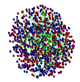
Figure 1: Pictorial representation of motion (green lines) of a particle on a noncommutative Riemann manifold.

The Bernoulli processes $B_{A}$ and the Wiener process $dX_{A}$ are not independent. We expect that the sign arising from the Bernoulli process should be the same of that of the corresponding Wiener process. This stochastic differential equation is the equivalent of the eq.(3) for the coordinates on the manifold. As we will see below, this is the same as the formula for the square root of a Wiener process. This represents the motion of a particle on a quantized noncommutative Riemann manifold. In this way, the Schrödinger equation can be removed from the state of a postulate and, underlying quantum mechanics, we have a quantized manifold.

III Fractional powers of Wiener processes

The first step is to prove the existence of the square root process. This was already accomplished in [11] using numerical techniques. Anyway, we give the following theorem here:

Theorem 1.

Given a random variable $X(t)\sim N(0,\sqrt{t})$, on a time sequence $\{t(m)\}\in\mathbb{R}$ and $m\in\mathbb{N}$, the sequence $Y(m+1)=Y(m)+\sqrt{X(m)}$ exists and belongs to $\mathbb{C}$. Then, $Y(t)$ on the same sequence, is a stochastic process representing the square root of a Brownian motion.

Proof.

Let us write $X(m)=|X(m)|e^{ik(m)\pi}$, being $\{k(m)\}$ a random sequence in $\mathbb{N}$ corresponding to $\operatorname{sgn}(X(m))$. Then, $\sqrt{X(m)}=\sqrt{|X(m)|}e^{ik(m)\frac{\pi}{2}}\in\mathbb{C}$ , exists and is well defined. Then, also the sequence $Y(m+1)=Y(m)+\sqrt{X(m)}$ exists and is well-defined and is in $\mathbb{C}$.

But the sequence $\{Y(i)\}$ represents the stepwise solution, through the Euler-Maruyama method, of the stochastic equation

$$dY=\sqrt{dX}$$ (13)

being $dX$ a Brownian process by construction. Now, being the Brownian process continuous, the limit of the time step $\Delta t=t(m+1)-t(m)\rightarrow 0$ also exists and so, the square root process exists as well. ∎

With Itō calculus we can express the “square root” process through more elementary stochastic processes [20], $(dW)^{2}=dt$, $dW\cdot dt=0$, $(dt)^{2}=0$ and $(dW)^{\alpha}=0$ for $\alpha>2$, we set

$$dX=(dW)^{\frac{1}{2}}\overset{?}{=}\left(\mu_{0}+\frac{1}{2\mu_{0}}dT-\frac{1}{8\mu_{0}^{3}}dt\right)\cdot\Phi_{\frac{1}{2}}$$ (14)

being $dT=dW\cdot\operatorname{sgn}(dW)$ a Tanaka process [21] such that $(dT)^{2}\sim(dW)^{2}\sim dt$, $\mu_{0}\neq 0$ an arbitrary scale factor and

$$\Phi_{\frac{1}{2}}=\frac{1-i}{2}\operatorname{sgn}(dW)+\frac{1+i}{2}$$ (15)

a Bernoulli process equivalent to a coin tossing that has the property $(\Phi_{\frac{1}{2}})^{2}=\operatorname{sgn}(dW)$. The possible outcomes for this process are $1$ and $i$ and represent a particle executing Brownian motion scattering two different kinds of small pieces of space, each one contributing either 1 or i to the process, randomly. We have already seen this process for the noncommutative geometry in eq.(11). We have introduced the process $\operatorname{sgn}(dW)$ that yields just the signs of the corresponding Wiener process. But Eq.(14) is not satisfactory for, taking the square, yields

$$(dX)^{2}=\mu_{0}^{2}\operatorname{sgn}(dW)+dW$$ (16)

and we do not exactly recover the original Wiener process. We see that we have added a process that has an overall effect to shift upward the original Brownian motion even if its shape is preserved.

This problem can be fixed by using the Clifford algebra formed by the Pauli matrices [19]. Taking two different Pauli matrices $\sigma_{i},\ \sigma_{k}$ with $i\neq k$ such that $\{\sigma_{i},\sigma_{k}\}=0$ we can rewrite the above identity as

$$I\cdot dX=I\cdot(dW)^{\frac{1}{2}}=\sigma_{i}\left(\mu_{0}+\frac{1}{2\mu_{0}}dT-\frac{1}{8\mu_{0}^{3}}dt\right)\cdot\Phi_{\frac{1}{2}}+i\sigma_{k}\mu_{0}\cdot\Phi_{\frac{1}{2}}$$ (17)

and so, $(dX)^{2}=dW$ as it should. This idea can be easily generalized to higher dimensions using Dirac’s $\gamma$ matrices. We see that we have recovered a similar stochastic process as in eq.(12).

This view agrees very well with the recent results by Connes, Chamseddine and Mukhanov [12, 13] and yields a hint for the underlying possible quantization of space.

We notice from this result that already the presence of the Tanaka process, that is defined in a weak sense [21], means that the square root process is a complex valued stochastic process not in a proper sense [17]. We will see this below.

For consistency reasons, we also provide the operational definitions for the involved processes needed to complete the above derivation. These are [11]

$$\operatorname{sgn}(dW)=\{\operatorname{sgn}(W_{0}),\operatorname{sgn}(W_{1}),\operatorname{sgn}(W_{2}),\ldots\}$$ (18)

such that $(\operatorname{sgn}(dW))^{2}=I$,

$$|dW|=\{|W_{0}|,|W_{1}|,|W_{2}|,\ldots\}$$ (19)

and for the Tanaka process

$$dT=|dW|\operatorname{sgn}(dW)=\{|W_{0}|\cdot\operatorname{sgn}(W_{0}),|W_{1}|\cdot\operatorname{sgn}(W_{1}),|W_{2}|\cdot\operatorname{sgn}(W_{2}),\ldots\}=dW.$$ (20)

These definitions are also used in the numerical evaluation for the proof by construction in Sec. V.

We can consider a more general “square root” process by adding a term proportional to $dt$. We take for granted that the Pauli matrices are used to remove the $\operatorname{sgn}$ so, we will permit us to neglect it. Assuming for the sake of simplicity $\mu_{0}=1/2$, one has

$$dX(t)=[dW(t)+\beta dt]^{\frac{1}{2}}=\left[\frac{1}{2}+dW(t)\cdot\operatorname{sgn}(dW(t))+(-1+\beta\operatorname{sgn}(dW(t)))dt\right]\Phi_{\frac{1}{2}}(t),$$ (21)

being $\beta$ an arbitrary constant. From the Bernoulli process $\Phi_{\frac{1}{2}}(t)$ one gets

$$\mu=-\frac{1+i}{2}+\beta\frac{1-i}{2}\qquad\sigma^{2}=2D=-\frac{i}{2}.$$ (22)

The presence of a complex valued pseudo-variance $\sigma^{2}$ show that the square root is an improper complex-valued process [17]. So, we have the following lemma:

Lemma 1.

A square root stochastic process is an improper complex-valued stochastic process.

Therefore, we have a double Fokker–Planck equation for a free particle, being the distribution function $\hat{\psi}$ complex valued,

$$\frac{\partial\hat{\psi}}{\partial t}=\left(\frac{1+i}{2}-\beta\frac{1-i}{2}\right)\frac{\partial\hat{\psi}}{\partial X}-\frac{i}{4}\frac{\partial^{2}\hat{\psi}}{\partial X^{2}}.$$ (23)

This result is not unexpected as, having complex random variables, we should have a Fokker–Planck equation for the real part and another for the imaginary part. The surprising result is that we get an equation strongly resembling the Schrödinger equation. We will see below that we are really recovering quantum mechanics, by recovering the heat kernel from the Monte Carlo simulation of the “square root” process, after a Wick rotation the square root process.

IV
Proof of the existence of the square root of the Brownian motion

In this section we will go deeper into the properties of the square root process, starting from the following theorem:

Theorem 2.

The square root of a standard Brownian motion can be given by

$$\sqrt{W\left(t\right)}=\frac{t^{\frac{1}{4}}}{2\left(E\Phi^{4}\right)^{\frac{1}{4}}}\left[\Phi-\mid\Phi\mid+i\left(\Phi+\mid\Phi\mid\right)\right],$$ (24)

where $\Phi$ is a real-valued continuous random variable, $E\Phi=0,$ $-\Phi\mid\Phi\mid\sim N\left(0,E\Phi^{4}\right),$ $i=\sqrt{-1,}$ and $t$ is time.

Proof.

First, in general, the process $\frac{t^{\frac{1}{4}}}{2\left(E\Phi^{4}\right)^{\frac{1}{4}}}\left[\Phi-\mid\Phi\mid+i\left(\Phi+\mid\Phi\mid\right)\right]$ exists since it is a (typical) complex random variable. To show that it is the square root of a Brownian motion in particular, we use $\left(\ref{1}\right)$ to get

$$W\left(t\right)=\left(\frac{t^{\frac{1}{4}}}{2\left(E\Phi^{4}\right)^{\frac{1}{4}}}\left[\Phi-\mid\Phi\mid+i\left(\Phi+\mid\Phi\mid\right)\right]\right)^{2}=-\frac{\sqrt{t}}{\sqrt{E\Phi^{4}}}\Phi\mid\Phi\mid.$$

Clearly, from the definition of a Brownian motion, the process $-\frac{\sqrt{t}}{\sqrt{E\Phi^{4}}}\Phi\mid\Phi\mid$ is a standard Brownian motions ($E\left[-\frac{\sqrt{t}}{\sqrt{E\Phi^{4}}}\Phi\mid\Phi\mid\right]=0$ and $Var\left(-\frac{\sqrt{t}}{\sqrt{E\Phi^{4}}}\Phi\mid\Phi\mid\right)$ $=t)$, since a Brownian motion is defined as $\sqrt{t}X$, where $X$ is a Gaussian variable. ∎

Similarly, using the same procedure, it can be shown that

$$\sqrt{dW\left(t\right)}=\frac{\left(dt\right)^{\frac{1}{4}}}{2\left(E\Psi^{4}\right)^{\frac{1}{4}}}\left[\Psi-\mid\Psi\mid+i\left(\Psi+\mid\Psi\mid\right)\right],$$

where $\Psi$ is a real-valued random variable so that $-\Psi\mid\Psi\mid\sim N\left(0,E\Psi^{4}\right).$

Properties.

The square root of the Brownian motion has some of the typical properties of a Brownian motion, such as

1. It is continuous almost surely.

   This follows directly from the continuity of $\Phi.$

2. It is nowhere differentiable almost surely.

   Proof.

   $d\sqrt{W\left(t\right)}=\frac{1}{2\sqrt{W\left(t\right)}}dW\left(t\right)+....$ Thus,

   $\frac{d\sqrt{W\left(t\right)}}{dt}=\frac{1}{2\sqrt{W\left(t\right)}}\frac{dW\left(t\right)}{dt}+...$ and $W\left(t\right)$ is nowhere differentiable. ∎

   This result is empirically verified in [11].

3. It starts from zero almost surely.

   This directly follows from $W\left(0\right)=0.$

4. Scaling: $c^{\frac{1}{4}}\sqrt{W\left(t/c\right)}$ $,c^{-\frac{1}{4}}\sqrt{W\left(ct\right)}$ and $\sqrt{W\left(t\right)}$ are square root Brownian motions, $c\neq 0.$ This follows directly from $\left(\ref{1}\right).$

5. However, unlike a Brownian motion,

   $$E\sqrt{W\left(t\right)}=\left(i-1\right)\frac{t^{\frac{1}{4}}}{2\left(E\Phi^{4}\right)^{\frac{1}{4}}}E\mid\Phi\mid$$

   and

   $$Var\left(\sqrt{W\left(t\right)}\right)=\frac{\sqrt{t}}{4\sqrt{E\Phi^{4}}}\left[Var\left(\Phi\right)+Var\left(\mid\Phi\mid\right)\right].$$

V Monte Carlo study

A recent Monte Carlo study by the authors [11] has shown the existence of fractional Wiener processes, provided a proper definition of the involved random evaluated functions is given. In this way, a straightforward numerical implementation is possible. Having this in mind, we use the same technique to perform a Monte Carlo evaluation of the diffusion process involved with our complex random processes and show that the so obtained mean, variance and probability distribution agree fairly well with what we have obtained theoretically so far. We just note that mean and variance should be evaluated by dividing by $\mu_{0}$ and $\mu_{0}^{2}$ respectively. $\mu_{0}$ should be chosen greater than one. In our case $\beta$, that appears in eq. (21), is assumed to be zero.

We performed a Monte Carlo study where each Brownian path is evaluated for 1000 steps for 20000 runs. In this way we were able to evaluate both the Wiener process, its square root and eq. (21) obtained by Euler-Maruyama method. We expect that the kernel is the standard heat kernel for the first case and a Schrödinger kernel otherwise. But this should be correlated by a Wick rotation. So, in order to perform a fit with a Gaussian distribution, we need to be certain that the phases of the Schrödinger kernel, producing the imaginary part, are removed after a Wick rotation. This is indeed the case. Therefore, given the set of random complex numbers $\psi$ obtained by numerically evaluating the square of a Wiener path sample, we evaluate the module $\rho$ and the phase $\theta$ for each one of them. Now we have for the Schrödinger kernel

$$\hat{\psi}=(4\pi it)^{-\frac{1}{2}}\exp{\left(ix^{2}/4t\right)}=(4\pi t)^{-\frac{1}{2}}\left[\cos\left(\frac{x^{2}}{4t}-\frac{\pi}{4}\right)+i\sin\left(\frac{x^{2}}{4t}-\frac{\pi}{4}\right)\right].$$ (25)

A Wick rotation, $t\rightarrow-it$, turns it into a heat kernel giving immediately

$$K=(4\pi t)^{-\frac{1}{2}}\left[\cos\left(i\frac{x^{2}}{4t}-i\frac{\pi}{4}\right)+i\sin\left(i\frac{x^{2}}{4t}-i\frac{\pi}{4}\right)\right]e^{\frac{\pi}{4}}.$$ (26)

Given the phases and modules computed by our set of samples, this can be easily expressed using them. The result is given in Fig. 2.

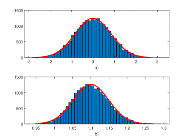
Figure 2: Comparison between the heat kernel a) and the Schrödinger kernel b) obtained after a Wick rotation.

One sees that one gets a perfect normal distribution in both the cases as it should. We just note that, in our case, the Schrödinger kernel has its center shifted, in agreement with our expectations.

In Fig. 3, we show the distributions of the averages and the variances of the square root of the Wiener process.

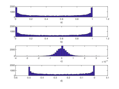
Figure 3: Distributions of the means (real part a) and imaginary part b)) and variances (real part c) and imaginary part d)) of the square root process.

In table 1, we report the values of their means, variances and diffusion coefficients.

Table 1: Means, variances and diffusion coefficients.

Process	Mean	Variance	Diffusion coefficient
Brownian	$-0.001\pm 0.004$	$0.1667\pm 0.0011$	$0.2041\pm 0.0013$
Square root	$0.4986\pm 0.0025+(0.5016\pm 0.0025)i$	$0\pm 4\cdot 10^{-7}-(0.2491\pm 0.0013)i$	$-(0.249\pm 0.001)i$

The agreement with our theoretical results, looking at eq. (23), is exceedingly good confirming that we are observing a diffusion process ruled by the Schrödinger equation arising from the square root of a Wiener process. Particularly, we notice the values $(1+i)/2$ for the mean of the square root process, in agreement with eq. (22) (in our numerical study is $\beta=0$), and the variance being $-i/4$ in agreement with the expected diffusion coefficient. This appears to be just Wick-rotated with respect to the case of the heat equation.

VI Conclusions

We have layed the theoretical and mathematical foundations of the square root of Browniam motion and we proved the existence of this process. We also have shown, also through a Monte Carlo study, the existence of a diffusion process, described by a Schrödinger equation, arising by taking the square root of an ordinary Brownian motion. We have a complete agreement with the theoretical expectations. As a concluding remark, we are pleased to note that our theory has recently been applied in the field of stock exchange prediction as a refinement of the Black and Scholes equation [18]. Therefore, this process will have many applications in economics. For example, it can be used to model stochastic volatility, stochastic interest rate and asset pricing, among others. Stochastic volatility is becoming increasingly popular in economics and econometrics. This is very timely, since econophysics is an emerging field. This paper can strengthen and help shape this new field of study.

A natural future extension of this paper is to introduce stochastic integrals for the square root of a Brownian motion and compare them to Ito’s integrals.

References

- [1]
- [2] E. Nelson, Dynamical Theories of Brownian Motion (Princeton University Press, Princeton, 1967).
- [3] F. Guerra “Structural Aspects Of Stochastic Mechanics And Stochastic Field Theory. (talk),” Phys. Rept. 77, 263 (1981).
- [4] H. Grabert, P. Hänggi, P. Talkner, Phys. Rev. A 19, 2440 (1979).
- [5] G. A. Skorobogatov, S. I. Svertilov, Phys. Rev. A 58, 3426 (1998).
- [6] P. Blanchard, S. Golin, M. Serva. Phys. Rev. D 34, 3732 (1986).
- [7] M. S. Wang, W.–K. Liang, Phys. Rev. D 48, 1875 (1993).
- [8] P. Blanchard, M. Serva, Phys. Rev. D 51, 3132 (1995).
- [9] A. Farina, M. Frasca, M. Sedehi, Signal Image Video Process. 8(1), 27-37 (2014).
- [10] M. Frasca, [arXiv:1201.5091 [math-ph]] (2012) unpublished.
- [11] M. Frasca, A. Farina, Signal Image Video Process. 11(7), 1365-1370 (2017) [arXiv:1403.1075 [math-ph]].
- [12] A. H. Chamseddine, A. Connes and V. Mukhanov, Phys. Rev. Lett. 114, no. 9, 091302 (2015) [arXiv:1409.2471 [hep-th]].
- [13] A. H. Chamseddine, A. Connes and V. Mukhanov, JHEP 1412, 098 (2014) [arXiv:1411.0977 [hep-th]].
- [14] M. Nakahara, Geometry, Topology and Physics (IOP Publishing, London, 2003).
- [15] K. B. Sinha, , D. Goswami, Quantum stochastic processes and noncommutative geometry. Cambridge Tracts in Mathematics, 169. (Cambridge University Press, Cambridge, 2007).
- [16] K. R. Parthasarathy, An introduction to quantum stochastic calculus. Monographs in Mathematics, 85. (Birkhäuser Verlag, Basel, 1992).
- [17] P. J. Schreier, L. L. Scharf, Statistical Signal Processing of Complex-Valued Data, Cambridge, Cambridge University Press, 2010. Definition 2.1 on page 35.
- [18] M. Alghalith, “Pricing options under simultaneous stochastic volatility and jumps: a simple closed formula without numerical/computational methods”, Physica A 540, 123100 (2020).
- [19] R. Delanghe, F. Sommen, V. Souček, Clifford Algebra and Spinor-Valued Functions - A Function Theory for the Dirac Operator (Springer, Berlin, 1992).
- [20] B. K. Øksendal, Stochastic Differential Equations: An Introduction with Applications, Berlin, Springer, 2003. Page 44.
- [21] B. K. Øksendal, ibid., page 71.