Case Study of the Proof of Cook’s theorem
- Interpretation of $A(w)$

Abstract

Cook’s theorem is commonly expressed such as any polynomial time-verifiable problem can be reduced to the SAT problem. The proof of Cook’s theorem consists in constructing a propositional formula $A(w)$ to simulate a computation of TM, and such $A(w)$ is claimed to be CNF to represent a polynomial time-verifiable problem $w$. In this paper, we investigate $A(w)$ through a very simple example and show that, $A(w)$ has just an appearance of CNF, but not a true logical form. This case study suggests that there exists the begging the question in Cook’s theorem.

8 2012 18 X. Liu et al. 1553–9105 January 2012 1

1 Introduction

Cook’s theorem [1] is now expressed as any polynomial time-verifiable problem can be reduced to the SAT (SATisfiability) problem. The proof of Cook’s theorem consists in simulating a computation of TM (Turing Machine) by constructing a propositional formula $A(w)$ that is claimed to be CNF (Conjonctive Normal Form) to represent the polynomial time-verifiable problem [1].

In this paper we investigate whether this $A(w)$ is a true logical form to represent a problem through a very simple example.

2 Example

2.1 Polynomial time-verifiable problem and Turing Machine

A polynomial time-verifiable problem refers to a problem $w$ for which there exists a Turing Machine $M$ to verify a certificat $u$ in polynomial time, that is, check whether $u$ is a solution to $w$.

Let us study a very simple polynomial time-verifiable problem :

Given a propositional formula $w=\neg x$ for which there exists a Turing Machine $M$ to verify whether a truth value $u$ of $x$ is a solution to $w$.

The transition function of $M$ can be represented as follows:

$q_{0}$	0	$\rightarrow$	1	$N$	$q_{1}$
$q_{0}$	1	$\rightarrow$	0	$N$	$q_{1}$
$q_{1}$	1	$\rightarrow$	1	$R$	$q_{Y}$
$q_{1}$	0	$\rightarrow$	0	$R$	$q_{N}$

where $N$ means that the tape head does not move, and $R$ means that the tape head moves to right; $q_{Y}$ refers to the state where $M$ stops and indicates that $u$ is a solution to $w$, and $q_{N}$ refers to the state where $M$ stops and indicates that $u$ is not a solution to $w$.

2.2 Computation of Turing Machine

A computation of $M$ consists of a sequence of configurations: $C(1),C(2),...,C(T)$, where $T=Q(\mid w\mid)$ and $Q(n)$ is a polynomial function. A configuration $C(t)$ represents the situation of $M$ at time $t$ where $M$ is in a state, with some symbols on its tape, with its head scanning a square, and the next configuration is determined by the transition function of $M$.

Fig.1 and Fig. 2 illustrate two computations of $M$ on inputs : $x=0$ and $x=1$.

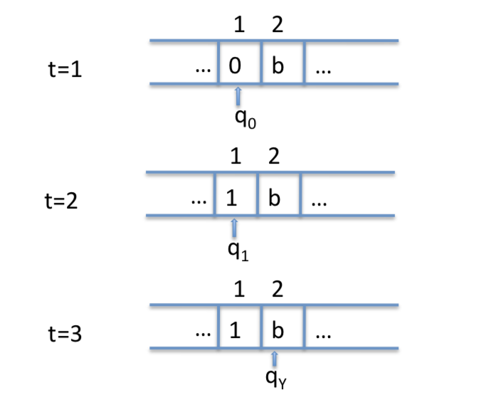
Figure 1: The computation on input $x=0$.

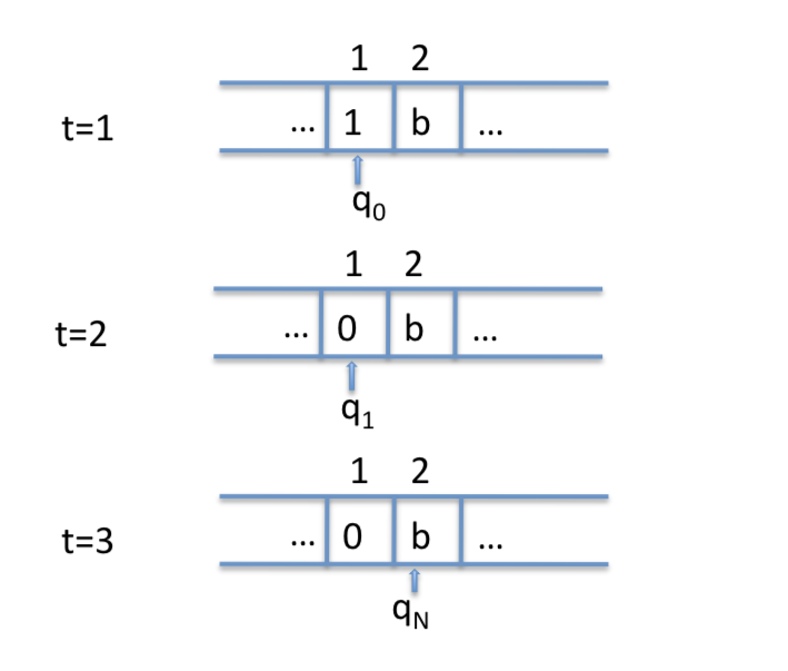
Figure 2: The computation on input $x=1$.

3 Form of $A(w)$

According to the proof of Cook’s theorem [1][2], the formula $A(w)$ is built by simulating a computation of $M$, such as $A(w)=B\land C\land D\land E\land F\land G\land H\land I$. $A(w)$ is claimed to represent a problem $w$.

We construct $A(w)$ for the above example.

3.1 Basic elements

The machine $M$ possesses:

• 4 states : $\{q_{0},q_{1},q_{2}=q_{Y},q_{3}=q_{N}\}$, where $q_{0}$ is the initial state, and $q_{2}$, $q_{3}$ are two final states.

• 3 symbols : $\{\sigma_{1}=b,\sigma_{2}=0,\sigma_{3}=1\}$, where $\sigma_{1}$ is the blank symbol.

• 2 square numbers : $\{s=1,s=2\}$.

• 4 rules.

• $n$ is the input size, $n=2$; $p(n)$ is a polynomial function of $n$, and $p(2)=3$.

• 3 times ($t=1,t=2,t=3$) et 2 steps to verify a certificat $u$ of $w$, where $t=1$ corresponds to the time for the initial state of the machine.

3.2 Proposition symbols

Three types of proposition symbols to represent a configuration of $M$ :

• $P_{s,t}^{i}$ for $1\leq i\leq 3$, $1\leq s\leq 2$, $1\leq t\leq 3$. $P_{s,t}^{i}$ is true iff at step $t$ the square number $s$ contains the symbol $\sigma_{i}$.

• $Q_{t}^{i}$ for $1\leq i\leq 4$, $1\leq t\leq 3$. $Q_{t}^{i}$ is true iff at step t the machine is in state $q_{i}$.

• $S_{s,t}$ for $1\leq s\leq 2$, $1\leq t\leq 3$ is true iff at step $t$ the tape head scans square number $s$.

3.3 Propositions

1. $E={E_{1}\land E_{2}\land E_{3}}$, where $E_{t}$ represents the truth values of $P_{s,t}^{i}$, $Q_{t}^{i}$ and $S_{s,t}$ at time $t$:

• $E_{1}=Q_{1}^{0}\land S_{1,1}\land P_{1,1}^{2}\land P_{2,1}^{1}$ ($x=0(\sigma_{2}$)); $E_{1}=Q_{1}^{0}\land S_{1,1}\land P_{1,1}^{3}\land P_{2,1}^{1}$ ($x=1(\sigma_{3}$))

• $E_{2}$ and $E_{2}$ are determined by the transition function of $M$

2. $B={B_{1}\land B_{2}\land B_{3}}$, where $B_{t}$ asserts that at time $t$ one and only one square is scanned :

• $B_{1}=(S_{1,1}\lor S_{2,1})\land(\neg S_{1,1}\lor\neg S_{2,1})$

• $B_{2}=(S_{1,2}\lor S_{2,2})\land(\neg S_{1,2}\lor\neg S_{2,2})$

• $B_{3}=(S_{1,3}\lor S_{2,3})\land(\neg S_{1,3}\lor\neg S_{2,3})$

3. $C={C_{1}\land C_{2}\land C_{3}}$, where $C_{t}$ asserts that at time $t$ there is one and only one symbol at each square. $C_{t}$ is the conjunction of all the $C_{i,t}$.

$C_{1}=C_{1,1}\land C_{2,1}$:

• $C_{1,1}=(P_{1,1}^{1}\lor P_{1,1}^{2}\lor P_{1,1}^{3})\land(\neg P_{1,1}^{1}\lor\neg P_{1,1}^{2})\land(\neg P_{1,1}^{1}\lor\neg P_{1,1}^{3})\land(\neg P_{1,1}^{2}\lor\neg P_{1,1}^{3})$

• $C_{2,1}=(P_{2,1}^{1}\lor P_{2,1}^{2}\lor P_{2,1}^{3})\land(\neg P_{2,1}^{1}\lor\neg P_{2,1}^{2})\land(\neg P_{2,1}^{1}\lor\neg P_{2,1}^{3})\land(\neg P_{2,1}^{2}\lor\neg P_{2,1}^{3})$

$C_{2}=C_{1,2}\land C_{2,2}$:

• $C_{1,2}=(P_{1,2}^{1}\lor P_{1,2}^{2}\lor P_{1,2}^{3})\land(\neg P_{1,2}^{1}\lor\neg P_{1,2}^{2})\land(\neg P_{1,2}^{1}\lor\neg P_{1,2}^{3})\land(\neg P_{1,2}^{2}\lor\neg P_{1,2}^{3})$

• $C_{2,2}=(P_{2,2}^{1}\lor P_{2,2}^{2}\lor P_{2,2}^{3})\land(\neg P_{2,2}^{1}\lor\neg P_{2,2}^{2})\land(\neg P_{2,2}^{1}\lor\neg P_{2,2}^{3})\land(\neg P_{2,2}^{2}\lor\neg P_{2,2}^{3})$

$C_{3}=C_{1,3}\land C_{2,3}$:

• $C_{1,3}=(P_{1,3}^{1}\lor P_{1,3}^{2}\lor P_{1,3}^{3})\land(\neg P_{1,3}^{1}\lor\neg P_{1,3}^{2})\land(\neg P_{1,3}^{1}\lor\neg P_{1,3}^{3})\land(\neg P_{1,3}^{2}\lor\neg P_{1,3}^{3})$

• $C_{2,3}=(P_{2,3}^{1}\lor P_{2,3}^{2}\lor P_{2,3}^{3})\land(\neg P_{2,3}^{1}\lor\neg P_{2,3}^{2})\land(\neg P_{2,3}^{1}\lor\neg P_{2,3}^{3})\land(\neg P_{2,3}^{2}\lor\neg P_{2,3}^{3})$

4. $D={D_{1}\land D_{2}\land D_{3}}$, where $D_{t}$ asserts that at time $t$ the machine is in one and only one state.

• $D_{1}=(Q_{1}^{0}\lor Q_{1}^{1}\lor Q_{1}^{2}\lor Q_{1}^{3})\land(\neg Q_{1}^{0}\lor\neg Q_{1}^{1})\land(\neg Q_{1}^{0}\lor\neg Q_{1}^{2})\land(\neg Q_{1}^{0}\lor\neg Q_{1}^{3})\land(\neg Q_{1}^{1}\lor\neg Q_{1}^{2})\land(\neg Q_{1}^{1}\lor\neg Q_{1}^{3})\land(\neg Q_{1}^{2}\lor\neg Q_{1}^{3})$

• $D_{2}=(Q_{2}^{0}\lor Q_{2}^{1}\lor Q_{2}^{2}\lor Q_{2}^{3})\land(\neg Q_{2}^{0}\lor\neg Q_{2}^{1})\land(\neg Q_{2}^{0}\lor\neg Q_{2}^{2})\land(\neg Q_{2}^{0}\lor\neg Q_{2}^{3})\land(\neg Q_{2}^{1}\lor\neg Q_{2}^{2})\land(\neg Q_{2}^{1}\lor\neg Q_{2}^{3})\land(\neg Q_{2}^{2}\lor\neg Q_{2}^{3})$

• $D_{3}=(Q_{3}^{0}\lor Q_{3}^{1}\lor Q_{3}^{2}\lor Q_{3}^{3})\land(\neg Q_{3}^{0}\lor\neg Q_{3}^{1})\land(\neg Q_{3}^{0}\lor\neg Q_{3}^{2})\land(\neg Q_{3}^{0}\lor\neg Q_{3}^{3})\land(\neg Q_{3}^{1}\lor\neg Q_{3}^{2})\land(\neg Q_{3}^{1}\lor\neg Q_{3}^{3})\land(\neg Q_{3}^{2}\lor\neg Q_{3}^{3})$

5. $F$, $G$, and $H$ assert that for each time $t$ the values of the $P_{s,t}^{i}$, $Q_{t}^{i}$ and $S_{s,t}$ are updated properly.

$F={F_{1}\land F_{2}}$, where $F_{t}$ is the conjunction over all $i$ and $j$ of $F_{i,j}^{t}$, where $F_{i,j}^{t}$ asserts that at time $t$ the machine is in state $q_{i}$ scanning symbol $\sigma_{j}$, then at time $t+1$ $\sigma_{j}$ is changed into $\sigma_{l}$, where $\sigma_{l}$ is the symbol given by the transition function for $M$.

$F_{1}=F_{0,2}^{1}\land F_{0,3}^{1}$ :

• $F_{0,2}^{1}=(\neg Q_{1}^{0}\lor\neg S_{1,1}\lor\neg P_{1,1}^{2}\lor P_{1,2}^{3})$, with the rule $(q_{0},0\rightarrow 1,N,q_{1})$

• $F_{0,3}^{1}=(\neg Q_{1}^{0}\lor\neg S_{1,1}\lor\neg P_{1,1}^{3}\lor P_{1,2}^{2})$, with the rule $(q_{0},1\rightarrow 0,N,q_{1})$

$F_{2}=F_{1,2}^{2}\land F_{1,3}^{2}$ :

• $F_{1,2}^{2}=(\neg Q_{2}^{1}\lor\neg S_{1,2}\lor\neg P_{1,2}^{2}\lor P_{1,2}^{2})$, with the rule $(q_{1},0\rightarrow 0,R,q_{N})$

• $F_{1,3}^{2}=(\neg Q_{2}^{1}\lor\neg S_{1,2}\lor\neg P_{1,2}^{3}\lor P_{1,3}^{3})$, with the rule $(q_{1},1\rightarrow 1,R,q_{Y})$

$G={G_{1}\land G_{2}}$, where $G_{t}$ is the conjunction over all $i$ and $j$ of $G_{i,j}^{t}$, where $G_{i,j}^{t}$ asserts that at time $t$ the machine is in state $q_{i}$ scanning symbol $\sigma_{j}$, then at time $t+1$ the machine is in state $q_{k}$, where $q_{k}$ is the state given by the transition function for $M$.

$G_{1}=G_{0,2}^{1}\land G_{0,3}^{1}$ :

• $G_{0,2}^{1}=(\neg Q_{1}^{0}\lor\neg S_{1,1}\lor\neg P_{1,1}^{2}\lor Q_{2}^{1})$, with the rule $(q_{0},0\rightarrow 1,N,q_{1})$

• $G_{0,3}^{1}=(\neg Q_{1}^{0}\lor\neg S_{1,1}\lor\neg P_{1,1}^{3}\lor Q_{2}^{1})$, with the rule $(q_{0},1\rightarrow 0,N,q_{1})$

$G_{2}=G_{1,2}^{2}\land G_{1,3}^{2}$ :

• $G_{1,2}^{2}=(\neg Q_{2}^{1}\lor\neg S_{1,2}\lor\neg P_{1,2}^{2}\lor Q_{3}^{3})$, with the rule $(q_{1},0\rightarrow 0,R,q_{N})$

• $G_{1,3}^{2}=(\neg Q_{2}^{1}\lor\neg S_{1,2}\lor\neg P_{1,3}^{3}\lor Q_{3}^{2})$, with the rule $(q_{1},1\rightarrow 1,R,q_{Y})$

$H={H_{1}\land H_{2}}$, where $H_{t}$ is the conjunction over all $i$ and $j$ of $G_{i,j}^{t}$, where $H_{i,j}^{t}$ asserts that at time $t$ the machine is in state $q_{i}$ scanning symbol $\sigma_{j}$, then at time $t+1$ the tape head moves according to the transition function for $M$.

$H_{1}=H_{0,2}^{1}\land H_{0,3}^{1}$ :

• $H_{0,2}^{1}=(\neg Q_{1}^{0}\lor\neg S_{1,1}\lor\neg P_{1,1}^{2}\lor S_{1,2})$, with the rule $(q_{0},0\rightarrow 1,N,q_{1})$

• $H_{0,3}^{1}=(\neg Q_{1}^{0}\lor\neg S_{1,1}\lor\neg P_{1,1}^{3}\lor S_{1,2})$, with the rule $(q_{0},1\rightarrow 0,N,q_{1})$

$H_{2}=H_{1,2}^{2}\land H_{1,3}^{2}$ :

• $H_{1,2}^{2}=(\neg Q_{2}^{1}\lor\neg S_{1,2}\lor\neg P_{1,2}^{2}\lor S_{2,3})$, with the rule $(q_{1},0\rightarrow 0,R,q_{N})$

• $H_{1,3}^{2}=(\neg Q_{2}^{1}\lor\neg S_{1,2}\lor\neg P_{1,3}^{3}\lor S_{2,3})$, with the rule $(q_{1},1\rightarrow 1,R,q_{Y})$

6. $I=(Q_{3}^{2}\lor Q_{3}^{3})\land(Q_{3}^{2}\lor\neg Q_{3}^{3})\land(\neg Q_{3}^{2}\lor Q_{3}^{3})$, asserts that the machine reaches the state $q_{y}$ or $q_{N}$ at time 3.

Finally, $A(w)=B\land C\land D\land E\land F\land G\land H\land I$.

4 Conjunctive form of $A(w)$

We develop $A(w)$ as a computation of $M$ for $x=0$ as input (see Fig. 1) in order to clarify the real sense of $A(w)$.

Let us define the configuration and the transition of configurations of $M$ :

$C(t)$ : the truth values of $P_{s,t}^{i}$, $Q_{t}^{i}$, $S_{s,t}$ and their constraints.

$C(t)\rightarrow C(t+1)$ : $C(t)$ is changed to $C(t+1)$ according to the transition function of $M$.

1. At $t=1$, $C(1)=E_{1}\land B_{1}\land C_{1}\land D_{1}$ :

• $E_{1}=Q_{1}^{0}\land S_{1,1}\land P_{1,1}^{2}\land P_{2,1}^{1}$, representing the initial configuration where $M$ is in $q_{0}$, the tape head scans the square of number 1, and a string $0b$ is on the tape.

• $B_{1}=(S_{1,1}\lor S_{2,1})\land(\neg S_{1,1}\lor\neg S_{2,1})$.

• $C_{1}=C_{1,1}\land C_{2,1}$:

  • $C_{1,1}=(P_{1,1}^{1}\lor P_{1,1}^{2}\lor P_{1,1}^{3})\land(\neg P_{1,1}^{1}\lor\neg P_{1,1}^{2})\land(\neg P_{1,1}^{1}\lor\neg P_{1,1}^{3})\land(\neg P_{1,1}^{2}\lor\neg P_{1,1}^{3})$

  • $C_{2,1}=(P_{2,1}^{1}\lor P_{2,1}^{2}\lor P_{2,1}^{3})\land(\neg P_{2,1}^{1}\lor\neg P_{2,1}^{2})\land(\neg P_{2,1}^{1}\lor\neg P_{2,1}^{3})\land(\neg P_{2,1}^{2}\lor\neg P_{2,1}^{3})$

• $D_{1}=(Q_{1}^{0}\lor Q_{1}^{1}\lor Q_{1}^{2}\lor Q_{1}^{3})\land(\neg Q_{1}^{0}\lor\neg Q_{1}^{1})\land(\neg Q_{1}^{0}\lor\neg Q_{1}^{2})\land(\neg Q_{1}^{0}\lor\neg Q_{1}^{3})\land(\neg Q_{1}^{1}\lor\neg Q_{1}^{2})\land(\neg Q_{1}^{1}\lor\neg Q_{1}^{3})\land(\neg Q_{1}^{2}\lor\neg Q_{1}^{3})$

2. At $t=2$, $C(2)=E_{2}\land B_{2}\land C_{2}\land D_{2}$ is obtained from $C(1)\land(C(1)\rightarrow C(2))$.

$C(1)\rightarrow C(2)$ is represented by $F$, $G$ and $H$ at $t=1$ :

- $F_{0,2}^{1}=(\neg Q_{1}^{0}\lor\neg S_{1,1}\lor\neg P_{1,1}^{2}\lor P_{1,2}^{3})$, with the rule $(q_{0},0\rightarrow 1,N,q_{1})$

- $G_{0,2}^{1}=(\neg Q_{1}^{0}\lor\neg S_{1,1}\lor\neg P_{1,1}^{2}\lor Q_{2}^{1})$, with the rule $(q_{0},0\rightarrow 1,N,q_{1})$

- $H_{0,2}^{1}=(\neg Q_{1}^{0}\lor\neg S_{1,1}\lor\neg P_{1,1}^{2}\lor S_{1,2})$, with the rule $(q_{0},0\rightarrow 1,N,q_{1})$

• $E_{2}=Q_{2}^{1}\land S_{1,1}\land P_{1,2}^{3}\land P_{2,2}^{1}$, with $Q_{2}^{1}=1$, $S_{1,2}=1$, $P_{1,2}^{3}=1$, $P_{2,2}^{1}=1$, and other proposition symbols concerning $t=2$ are assigned with 0.

• $B_{2}=(S_{1,2}\lor S_{2,2})\land(\neg S_{1,2}\lor\neg S_{2,2})$

• $C_{2}=C_{1,2}\land C_{2,2}$:

  • $C_{1,2}=(P_{1,2}^{1}\lor P_{1,2}^{2}\lor P_{1,2}^{3})\land(\neg P_{1,2}^{1}\lor\neg P_{1,2}^{2})\land(\neg P_{1,2}^{1}\lor\neg P_{1,2}^{3})\land(\neg P_{1,2}^{2}\lor\neg P_{1,2}^{3})$

  • $C_{2,2}=(P_{2,2}^{1}\lor P_{2,2}^{2}\lor P_{2,2}^{3})\land(\neg P_{2,2}^{1}\lor\neg P_{2,2}^{2})\land(\neg P_{2,2}^{1}\lor\neg P_{2,2}^{3})\land(\neg P_{2,2}^{2}\lor\neg P_{2,2}^{3})$

• $D_{2}=(Q_{2}^{0}\lor Q_{2}^{1}\lor Q_{2}^{2}\lor Q_{2}^{3})\land(\neg Q_{2}^{0}\lor\neg Q_{2}^{1})\land(\neg Q_{2}^{0}\lor\neg Q_{2}^{2})\land(\neg Q_{2}^{0}\lor\neg Q_{2}^{3})\land(\neg Q_{2}^{1}\lor\neg Q_{2}^{2})\land(\neg Q_{2}^{1}\lor\neg Q_{2}^{3})\land(\neg Q_{2}^{2}\lor\neg Q_{2}^{3})$

3. At $t=3$, $C(3)=E_{3}\land B_{3}\land C_{3}\land D_{3}$ is obtained from $C(2)\land(C(2)\rightarrow C(3))$.

$C(2)\rightarrow C(3)$ is represented by $F$, $G$ and $H$ at $t=2$ :

$F_{1,3}^{2}=(\neg Q_{2}^{1}\lor\neg S_{1,2}\lor\neg P_{1,2}^{3}\lor P_{1,3}^{3})$, with the rule $(q_{1},1\rightarrow 1,R,q_{Y})$

$G_{1,3}^{2}=(\neg Q_{2}^{1}\lor\neg S_{1,2}\lor\neg P_{1,3}^{3}\lor Q_{3}^{2})$, with the rule $(q_{1},1\rightarrow 1,R,q_{Y})$

$H_{1,3}^{2}=(\neg Q_{2}^{1}\lor\neg S_{1,2}\lor\neg P_{1,3}^{3}\lor S_{2,3})$, with the rule $(q_{1},1\rightarrow 1,R,q_{Y})$

• $E_{3}=Q_{3}^{2}\land S_{2,3}\land P_{1,3}^{3}\land P_{2,3}^{1}$, with $Q_{3}^{2}=1$, $S_{2,3}=1$, $P_{1,3}^{3}=1$, $P_{2,3}^{1}=1$ , and other proposition symbols concerning $t=3$ are assigned with 0.

• $B_{3}=(S_{1,3}\lor S_{2,3})\land(\neg S_{1,3}\lor\neg S_{2,3})$

• $C_{3}=C_{1,3}\land C_{2,3}$:

  • $C_{1,3}=(P_{1,3}^{1}\lor P_{1,3}^{2}\lor P_{1,3}^{3})\land(\neg P_{1,3}^{1}\lor\neg P_{1,3}^{2})\land(\neg P_{1,3}^{1}\lor\neg P_{1,3}^{3})\land(\neg P_{1,3}^{2}\lor\neg P_{1,3}^{3})$

  • $C_{2,3}=(P_{2,3}^{1}\lor P_{2,3}^{2}\lor P_{2,3}^{3})\land(\neg P_{2,3}^{1}\lor\neg P_{2,3}^{2})\land(\neg P_{2,3}^{1}\lor\neg P_{2,3}^{3})\land(\neg P_{2,3}^{2}\lor\neg P_{2,3}^{3})$

• $D_{3}=(Q_{3}^{0}\lor Q_{3}^{1}\lor Q_{3}^{2}\lor Q_{3}^{3})\land(\neg Q_{3}^{0}\lor\neg Q_{3}^{1})\land(\neg Q_{3}^{0}\lor\neg Q_{3}^{2})\land(\neg Q_{3}^{0}\lor\neg Q_{3}^{3})\land(\neg Q_{3}^{1}\lor\neg Q_{3}^{2})\land(\neg Q_{3}^{1}\lor\neg Q_{3}^{3})\land(\neg Q_{3}^{2}\lor\neg Q_{3}^{3})$
  

Therefore, the computation of $M$ for $x=0$ as input can be represented as :

$C(1)\land(C(1)\rightarrow C(2))\land(C(2)\rightarrow C(3))\\ =C(1)\land C(2)\land C(3)\\ =(E_{1}\land B_{1}\land C_{1}\land D_{1})\land(E_{2}\land B_{2}\land C_{2}\land D_{2})\land(E_{3}\land B_{3}\land C_{3}\land D_{3})\\ =E\land B\land C\land D\\ =A(w)$

It can be seen that $A(w)$ is just the conjonction of all configurations of $M$ to simulate a concret computation of $M$ for verifying a certificat $u$ of $w$. Given an input $u$ ($x=0$ or $x=1$ in this example), whether $M$ accepts it or not, $A(w)$ is always true. Obviously, $A(w)$ has just an appearance of conjunctive form, but not a true logical form.

5 Conclusion

In fact, a true CNF formula is implied in the transition function of $M$ corresponding to $F$, $G$, $H$ as well as $C(t)\rightarrow C(t+1)$, however the transition function of $M$ is based on the expressible logical structure of a problem.

Therefore, it is not that any polynomial time-verifiable problem can be reduced to the SAT problem, but any polynomial time-verifiable problem itself asserts that such problem is representable by a CNF formula. In other words, there exists the begging the question in Cook’s theorem.

References

- [1] Stephen Cook, The complexity of theorem proving procedures. Proceedings of the Third Annual ACM Symposium on Theory of Computing. p151-158 (1971)
- [2] Garey Michael R., David S. Johnson, Computers and Intractability: A Guide to the Theory of NP-Completeness. W. H. Freeman and company (1979)