1

Recurrent Neural Networks in the Eye of Differential Equations

Murphy Yuezhen Niu^1,2,3, Isaac L. Chuang^1,2, Lior Horesh^4,5
1Department of Physics, Massachusetts Institute of Technology, 77 Massachusetts Avenue, Cambridge, MA, 02139
²Research Laboratory of Electronics, Massachusetts Institute of Technology, 77 Massachusetts Avenue, Cambridge, MA, 02139
³Google Inc., 340 Main Street, Venice, CA 90291
⁴Mathematics of AI, IBM Research, Yorktown Height, NY 10598
⁵MIT-IBM Watson AI Lab, Cambridge, MA 02142

Keywords: recurrent neural network, ordinary differential equation, Runge-Kutta method, stability analysis, temporal dynamics of Neural Networks

To understand the fundamental trade-offs between training stability, temporal dynamics and architectural complexity of recurrent Neural Networks (RNNs), we directly analyze RNN architectures using numerical methods of ordinary differential equations (ODEs). We define a general family of RNNs–the ODERNNs–by relating the composition rules of RNNs to integration methods of ODEs at discrete time steps. We show that the degree of RNN’s functional nonlinearity $n$ and the range of its temporal memory $t$ can be mapped to the corresponding stage of Runge-Kutta recursion and the order of time-derivative of the ODEs. We prove that popular RNN architectures, such as LSTM and URNN, fit into different orders of $n$-$t$-ODERNNs. This exact correspondence between RNN and ODE helps us to establish the sufficient conditions for RNN training stability and facilitates more flexible top-down designs of new RNN architectures using large varieties of toolboxes from numerical integration of ODEs. We provide such an example: Quantum-inspired Universal computing Neural Network (QUNN), which reduces the required number of training parameters from polynomial in both data length and temporal memory length to only linear in temporal memory length.

1 Introduction

Exciting progress (Haber and Ruthotto, 2017; Lu et al., 2017; Ruthotto et al., 2018; Chen et al., 2018) has been made to unveil the common nature behind various transformations used in machine learning models, such as Neural Networks Haykin (1994) and normalizing flows (Rezende and Mohamed, 2015), realized by a sequence of transformations between hidden states: these iterative updates can be viewed as integration of either discrete or continuous differential equations. Such startling correspondence not only deepens our understanding of the inner workings of neural network based machine learning algorithms, but also offer advanced numerical integration methods obtained over the past century to the design of better learning architectures.

Haber et. al. are the first to map the residual neural network’s (ResNet’s) composition rules between hidden variables to the Euler discretization of continuous differential equations, and the stability of ResNet training to the stability of the equivalent numerical integration methods. Leveraging such mapping, they significantly improve ResNet’s stability by choosing the appropriate weight matrices whose spectrum properties guarantee its stable propagation. However, their analysis is limited to one kind of numerical integration method applied to ResNet. More recently, Chen et. al. replace the conventional neural network with its continuous limit: ordinary differential equations (ODEs). These neural ODEs enjoy many advantages over conventional Neural Networks: back-propagation is replaced by integration of conjugate variables representing the gradients of the hidden variables; stability is improved with the use of adaptive numerical integration methods for ODEs; it can learn efficiently from time-sequential data that are generated at unevenly separated physical times; and other improvements in the parameter and memory efficiencies. Yet such fully continuous extension of neural network also faces its own challenges: it is inconvenient to use mini-batches with neural ODEs; specific error in the backward integration of conjugate variable for state trajectory reconstruction can be amplified, and neural ODE’s large scale implementation cannot directly benefit from the emerging hardware developed for tensor multiplication.

Since temporal discretization is nonetheless unavoidable in the machine-level integration of ODEs, why not keep the neural network paradigm but include a larger family of ODE integration methods in addition to Euler discretization? A more generalized correspondence will open the door to complex neural network architectures inspired by physical dynamics represented by ODEs. In particular, we are interested in recurrent Neural Networks (RNNs) for their generality (conventional deep Neural Networks can be regarded as the trivial type of RNN with trivial recurrence) and their capability to learn complex dynamics that require temporal memories.

As indispensable tools for machine translation, robotic control, speech recognition and various time-sequential tasks, RNNs are nonetheless limited in their application due to their susceptibility to training instability that can be amplified by the recurrent connectivity. Various architectural redesigns are introduced to mitigate this problem (Hochreiter and Schmidhuber, 1997; Cho et al., 2014; Wermter et al., 1999; Jaeger et al., 2007; Bengio et al., 2013; Cho et al., 2014; Koutnik et al., 2014; Mhaskar and Poggio, 2016; Arjovsky et al., 2016b; Jing et al., 2016). These improved stability guarantees also come with an expense of additional architectural complexity  (Jozefowicz et al., 2015; Karpathy et al., 2015; Alpay et al., 2016; Greff et al., 2017). They point to an underlying trade-off between the stability, temporal dynamics and architectural complexity of RNN that is yet to be found. Establishing specific connections between more general ODE methods with composition rules of RNN architectures can be the first step towards understanding this stability-complexity trade-off.

In fact, Runge-Kutta methods (Runge, 1895; Kutta, 1901) are generalizations to Euler’s method, which numerically solve ODEs with higher orders of functional non-linearity through higher stages of recursion in their discrete integration rules. Since a higher order time-derivative can be transformed to coupled first order ODEs, an $n$-stage Runge-Kutta with $t$-coupled variables thus represents a $t$th order ODE with $n$th order temporal non-linearity. Different orders of Runge-Kutta methods not only facilitate different orders of convergence guarantees to the numerical integration; they also provide a simple but accurate understanding of the underlying dynamics embodied by the ODEs.

In this work, we establish critical connections between RNN and ODE: the temporal dynamics of RNN architectures can be represented by a specific numerical integration method for a set of ODEs of a given order. Our result elucidates a fundamental trade-off between training stability, temporal dynamics, and architectural complexity of RNN: network’s stability and complexity of temporal dynamics can be increased by increasing the length of temporal memory (Koutnik et al., 2014) and the degree of temporal non-linearity, which on the other hand demands more non-local composition rules and thus higher complexity of the network architecture as predicted by the corresponding ODE integration method. This insight has practical implications when applying RNNs to real-world problems. On the one hand, additional information about the training data, such as its temporal correlation length obtained by lower level prepossessing, can be valuable for the choice of RNN architectures. On the other hand, one can design unconventional RNN architectures inspired by ODE counterparts for increased ability to represent complex temporal dynamics. For example, as opposed to autonomous ODEs which do not explicitly depend on the physical time of the incoming temporal data, RNNs based on non-autonomous dynamical ODEs have weight matrices specifically dependent on the input at each iteration after the training, or more concisely are dynamical. This captures and generalizes now-common extensions to traditional RNN structures, such as in the Neural Turing machine (Graves et al., 2014) which adds a write and read gated function to the data-independent network to facilitate the learning of arbitrary procedures. Illustrating the potential of this direction, we provide here one such dynamical weight RNN construction, inspired by a quantum algorithm for realizing universal quantum computation through the preparation of the ground state of a ”clock-Hamiltonian” (Aharonov et al., 2008). A clock-Hamiltonian represents the dynamical map between input and output of each temporal update, and is therefore specifically input dependent.

Using this specific correspondence between general ODE integration methods and RNN composition rules, we also identify a new property about RNN architecture: the order of non-linearity in its represented temporal dynamics. Traditionally, the stability of RNN is considered only with respect to its memory scale–represented by the order of time-derivatives in discrete ODEs. However, we realized that the range of connectivity between hidden layers in RNN can also affect the order of temporal non-linearity reflected in different stage of Runge-Kutta recursion. This offers us an additional insight to the inner workings of RNNs that is helpful for designing more suitable architectures given partial knowledge of the underlying physical dynamics of the data.

The structure of the paper are summarized as follows. In Sec. 2 we identify RNN’s temporal memory scale $t$ and the degree of non-linearity $n$ to its underlying architecture through an explicit correspondence to ODEs, by analyzing the discrete ODEs integration method that matches the RNN composition rules between hidden variables. We show that $t$ and $n$ are respectively determined by the order of time-derivative and the order of non-linearity of the ODEs that represent the RNN’s dynamics. We also provide sufficient condition for training stability for any $n$-$t$-ODERNN. Existing RNN architectures can thus be comprehended on the same ground according to their memory scale and the non-linearity of their dynamics (Table. 1). In Sec. 3 we provide an example of constructing new RNN architectures by choosing the appropriate underlying ODE dynamics first: Quantum inspired Universal computing recurrent Neural Network (QUNN). QUNN is unconventional in its specific time-dependence in the weight matrix construction. The number of training parameters in QUNN grows linearly with the temporal correlation length between input data which is otherwise independent of the dimension of data itself. We discuss the implication of our results in Sec. 4.

LSTM	GRU	URNN	CW-RNN	QUNN
$2$-$L$-ODERNN	$2$-$L$-ODERNN	$2$-$L$-ODERNN	$L$-$L$-ODERNN	$L$-$L$-ODERNN

Table 1: Categorization of RNN architectures according to their temporal memory scale and their order of non-linearity. LSTM (Hochreiter and Schmidhuber, 1997): long-term short-term memory RNN with $L$ hidden layers. GRU (Cho et al., 2014): gate model recurrent neural network with $L$ hidden layers. URNN (Arjovsky et al., 2016b): unitary evolution recurrent neural network with $L$ hidden layers. CW-RNN (Koutnik et al., 2014): clockwork recurrent neural network with $L$ hidden layers. QUNN: quantum universal computing recurrent neural network with $L$ hidden layers. $n$-$t$-ODERNN: recurrent neural network whose temporal dynamics is represented by a discrete integration of $t^{th}$ order ODE recursion relation using $n^{th}$ order recursion methods.

2 Stable Recurrent Neural Network

The success of supervised machine learning techniques depends on the stability, the representability and the computational overhead associated with the proposed training architecture and training data. Careful engineering of network’s architectures are necessary to realize these desirable properties since a generic neural network without any structure is susceptible to exploding or vanishing gradients (Bengio et al., 1994; Pascanu et al., 2013).

The groundbreaking work by Haber et. al. (Haber and Ruthotto, 2017) provides an elegant solution to guaranteeing the stability of deep Neural Networks: understand the neural network forward and backward propagation as a form of integration of discrete ODEs. As an example, we look at a type of ResNet proposed in (Haber and Ruthotto, 2017). Let $l^{th}$ layer of hidden variable be $Y_{l}\in\mathcal{R}^{s\times p}$ and bias be $b_{l}\in\mathcal{R}^{s\times p}$, to ensure the stability of propagation. They introduce a conjugate variable $Z_{l\pm\frac{1}{2}}\in\mathcal{R}^{s\times p}$ as a intermediate step such that the propagation of neural network is described by

$$Z_{l+\frac{1}{2}}=Z_{l-\frac{1}{2}}-h_{l}\sigma(W_{l}^{\top}Y_{l}+b_{l}),\,\,Y_{l+1}=Y_{l}+\sigma(W_{l}Z_{l+\frac{1}{2}}+b_{l}).$$ (1)

The dynamics of the above discrete ODE is stable regardless of the form of weight matrix $W_{l}$ (Haber and Ruthotto, 2017).

If RNN can be trained to represent temporal structures of physical data, its stability and complexity should also be understandable through the physical dynamics represented by ODEs. We generalized the method by Haber and Ruthotto (2017) introduced above to include higher order non-linearity and higher order time-derivative ODEs and to apply it larger family of neural network that include existing architectures of RNNs as special cases. We define an ODE recurrent neural network with $n^{th}$ order in non-linearity and $t^{th}$ order in time-derivative  ($n$-$t$-ODERNN) according to its propagation rule: the update of $n$-$t$-ODERNN can be mapped to a generalized $n$-stage Runge–Kutta integration with $t$ coupled variables. The specific choice of Runge-Kutta method is not essential to such generalization, and can be replaced by other integration method that provides different architecture ansatz. Such generalization help us to provide a sufficient condition for the stability criteria for any $n$-$t$-ODERNN. We then categorize several existing RNN architectures into different $n$-$t$-ODERNN according to their temporal memory scale and degree of non-linearity. Lastly, we define the $n$-$2$-ODERNN with anti-Hermitian weight matrices as $n$-ARNN and prove the stability of 1-ARNN and 2-ARNN.

2.1 $n^{th}$ order ODE Recurrent Neural Network

Definition 1. An ODE recurrent neural network of $n^{th}$ order in non-linearity $t^{th}$ order in gradient ($n$-$t$-ODERNN), with integers $n,t\geq 1$ and $k\in[n]$, is described by the update rule between input state value $Y_{l}\in\mathcal{R}^{s}$ at time step $l$, the hidden variables of the $k^{th}$ layer as $K_{k}\in\mathcal{R}^{p}$ with $1\leq k\leq n$, and output state value $Y_{l+1}\in\mathcal{R}^{s}$ as

$$K_{1}=\sigma_{1}\left(W_{1}Y_{l}+b_{1}\right),$$ (2)

$$K_{q}=\gamma_{q}K_{q-1}+\kappa_{q}\sigma_{q}\left(W_{q}Y_{l-t_{q-1}}+b_{q}+h\sum_{k=1}^{n}\alpha_{q,k}K_{k}\right),$$ (3)

$$Y_{l+1}=\gamma_{n+1}Y_{l}+\kappa_{n+1}\sigma_{q+1}\left(W_{n+1}Y_{l-t_{n-1}}+b_{n+1}+h\sum_{k=1}^{n}\beta_{k}K_{k}\right)$$ (4)

where $2\leq q\leq n$; the time corresponding to each hidden layer obeys $t_{k}=\lfloor t\frac{k}{n}\rfloor$ with the number of inputs in time coupled by the $n$ hidden layers being $t$; the point-wise activation function $\sigma_{*}(\circ):\mathcal{R}^{p}\to\mathcal{R}^{p}$ at each layer is a nonlinear map that preserves the dimension of the input; the weight matrix at each layer is represented by $W_{q}\in\mathcal{R}^{q_{2}\times q_{1}}$ where $q_{1}$ is the dimension of the input variable and $q_{2}$ is the dimension of the output variable of that layer; the scalar constant $h$ changes the rate of update of hidden variables between layers, the vector $b_{q}$ is the bias for the $q$th hidden layer, $\beta_{k},\gamma_{q},\kappa_{q}$ and $\alpha_{q,k}\in\mathcal{R}^{p\times p}$ are matrices served to rescale and rotate the hidden variables.

To facilitate later discussions based on Definition 1, we name $\alpha_{q,k}$ the Runge–Kutta matrix and $\{\beta_{k}\}$ the Runge-Kutta weight matrices following similar notation in the numerical integration of ODEs. Lastly, we define Burrage-Butcher tensor $Q$ named after its first inventors with each element defined by

$$Q_{i,j}=\beta_{i}\alpha_{ij}+\beta_{j}\alpha_{ji}-\beta_{i}\beta_{j}^{\top}$$ (5)

which will be an important quantity in the stability analysis of the represented dynamics to be discussed in Theorem 1.

Example $2$-$2$-ODERNN . A $2$-$2$-ODERNN is a four layer RNN with two hidden layers that obey the composition rules:

$$K_{1}=\sigma_{1}\left(W_{1}Y_{l}+b_{1}\right),$$ (6)

$$K_{2}=\gamma_{2}K_{1}+\kappa_{2}\sigma_{2}\left(W_{2}Y_{l-1}+b_{2}+h\alpha_{2,1}K_{1}\right),$$ (7)

$$Y_{l+1}=\gamma_{3}Y_{l}+\kappa_{3}\sigma_{3}\left(W_{3}Y_{l-1}+b_{3}+h\sum_{k=1}^{2}\beta_{k}K_{k}\right)$$ (8)

which is illustrated in Fig. 1. In comparison the connectivity for LSTM is represented in Fig. 2, where the connection between input and output in Fig. 1 is replaced by the output gate $o_{t}$, the first hidden layer $K_{1}$ is replaced by forget gate, and the second hidden layer $K_{2}$ is replaced by input gate and memory cell.

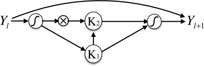
Figure 1: Diagrammatic representation of $2$-$2$-ODERNN, where the $\int$ sign inside a circle represents the nonlinear activation function, and the $\otimes$ represents the time-delayed feed forward. Each arrow represent the multiplication by a re-scaling factor: $\gamma_{3}$ for the arrow from $Y_{l}$ to $Y_{l+1}$, $\kappa_{2}$ for the arrow from $\int$ sign to $K_{1}$ , $\gamma_{2}$ for the arrow from $K_{1}$ to $K_{2}$, and $\beta_{k}$ for the arrow from $K_{k}$ to $\int$ sign.

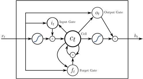
Figure 2: Diagrammatic representation of peehole LSTM taken from Wikipedia (2019), where the $\int$ sign inside a circle represents the nonlinear activation function, and the $\otimes$ represents the time-delayed feed forward.

Definition 1 can be compared with the explicit or implicit Runge-Kutta method for solving $\frac{d}{dt}\vec{y}=f(\vec{y},t)$ where the vector $\vec{y}$ is an unknown function of time that ODE solution provides. Recall that a $t$th order ODE can be mapped to the first order ODE with $\vec{y}$ of length $t$, each element of which is proportional to different order of discrete time derivative of the original variable. The $n$-stage explicit or implicit Rugge-Kutta method can be generalized to the following form for the solution to the ODE at the discrete time $t_{k}$ with time step $t_{k}-t_{k-1}=\delta$ given the solution $\vec{y}_{k-1}$ at the previous time step through the following iteration:

$$\vec{y}_{k}=\vec{y}_{k-1}+\delta\sum_{i=1}^{n}e_{i}\vec{k}_{i}$$ (9)

$$\vec{k}_{q}=f(d_{q}\vec{y}_{k-1}+\sum_{j=1}^{n}\delta a_{qj}\vec{k}_{j},t_{k-1}+c_{q}\delta)$$ (10)

where $a_{q,j},e_{i},c_{q},d_{q}$ are square matrices and determine the corresponding integration method. For example, if we set $a_{q,j}=0$ for all $q\leq j$, it gives us an explicit Runge-Kutta method, otherwise it corresponds to an implicit Runge-Kutta method. The difference between the two methods is in the additional requirement of solving the linear dependence of $\{\vec{k}_{q}\}$ in each iteration of implicit method, which lower the requirements on $f()$ for the numerical stability of the integration. If we treat the $k$th hidden layer from the ODERNN as the $k$th stage of integration method above, and choose the matrix $d_{k}$ to pick out the $k$th derivative which in discrete time-step corresponds to the variable separated by $k\delta$, the order of time derivative and the order of functional non-linearity of $n$-$t$-ODERNN becomes self-evident.

With this explicit connection, we can directly apply the stability analysis of Runge-Kutta method to the ODERNN with Theorem 1, which utilizes the notion of BN-stability specified below in Definition 2. BN-stability was first proposed by (Dahlquist, 1979) to investigate stability of numerical schemes applied to nonlinear systems satisfying a monotonicity condition, which is a generalization of the “A” stability for linear systems and widely used in analyzing the stability of high order Runge-Kutta methods.

Definition 2.The integration method for solving the nonlinear discretized ODE system of equations $\dot{\vec{y}}=f(\vec{y},t)$ is BN-stable if it satisfies the following requirements. It is monotonic: the inner product between the variable vector and the function vector is non-negative $\langle f(\vec{x},t)-f(\vec{y},t),\vec{x}-\vec{y}\rangle\leq 0$ for $t\geq 0;\vec{x},\vec{y}\in\mathcal{R}^{s}$; and a small perturbation at the initial state $\vec{y^{\prime}}_{0}=\vec{y}_{0}+\delta_{0}$ does not amplify as step size increases: for any $k$

$$||\vec{y}_{k-1}-\vec{y^{\prime}}_{k-1}||\leq||\vec{y}_{k}-\vec{y^{\prime}}_{k}||.$$ (11)

Based on Definition 2, we are ready to provide a stability guarantee for the ODERNNs in the following theorem.

Theorem 1. An $n$-$t$-ODERNN given by Eq. (6) is BN-stable if it satisfies the following conditions:

1. The Burrage-Butcher tensor $Q$ is positive semi-definite.

2. For any $k\in[n]$, the matrix $\beta_{k}$ is positive semi-definite.

Proof: Since the composition rule of $n$-$t$-ODERNN can be mapped to that of an $n$ stage general implicit Runge-Kutta method, the BN-stability proof for Theorem 1.4 from Spijker (1980) directly applies. The monotonicity requirement (Dahlquist, 1979) in Definition 2 is not sensitive to the gradient of the function and can also be replaced by $\langle f(\vec{x},t)-f(\vec{y},t)$, where we use $\vec{x}$ and $\vec{y}$ to represent the input and output of each hidden layer of RNN, which obeys $\langle\vec{x}-\vec{y}\rangle\geq 0$ for $t\geq 0;\vec{x},\vec{y}\in\mathcal{R}^{s}$, which is naturally satisfied by the rectified linear function or tanh.

2.2 Categorization of Existing RNNs

We apply this ODERNN framework to analyze some of the most widely used RNN architectures in regard to their non-linearity and memory scale of their underlying dynamics.

	traditional RNN (LSTM)	physical RNN (ODERNN)
$Y_{l}$	input at time step $l$	state variable at time step $l$
$K_{l_{j}}$	$j^{th}$ hidden layer	$j^{th}$ order increment of the gradient slope
$\gamma_{l_{j}}$	forget gate activation	energy dissipation rate
$\alpha_{i,j}$	weight matrix for hidden variable	weight of $i^{th}$ increment in $j^{th}$ order slope
$\kappa_{l_{j}}$	input gate’s activation	re-scale factor of normalized gradient function
$\sigma_{l_{j}}$	activation function of $j^{th}$ hidden layer	gradient function

Table 2: Comparison of the LSTM architecture and $n^{th}$ order ODERNN structure.

Definition 3. A LSTM with $L$ non-trivial hidden layers $\{K^{l}_{t}\},$ with $l\in[L]$, at time step $t$ obeys the following propagation rules between hidden variables. Each $K^{l}_{t}$ is of dimension $n$ and is updated at each time step as follows:

$$\left(\begin{matrix}i\\ f\\ o\\ g\end{matrix}\right)=\left(\begin{matrix}\sigma_{1}\\ \sigma_{2}\\ \sigma_{3}\\ \sigma_{4}\end{matrix}\right)W^{l}\left(\begin{matrix}K_{t}^{l-1}\\ K_{t-1}^{l}\end{matrix}\right)$$ (12)

$$c_{t}^{l}=f\circ c_{t-1}^{l}+i\circ g$$ (13)

$$K_{t}^{l}=o\circ\tanh(c_{t}^{l})$$ (14)

where $W^{l}$ is of dimension $4n\times 2n$, $\circ$ represents the element-wise product, and the four vectors, $i,f,o,g$ each of dimension $n$, with the first three controlling which input will be saved to influence the future output according to the above update rules in Eq. (13) and (14).

Claim 1. For any LSTM with $L$ hidden layers in Definition 3, there exists a 2-$L$-ODERNN that realizes the same input-output relation.

Proof: For one layer RNN, we have the update rule for LSTM (Hochreiter and Schmidhuber, 1997) as:

$$K_{t}=f_{t}\circ K_{t-1}+i_{t}\circ\sigma_{2}(W_{c}Y_{t-1}+U_{c}K_{t-1}+b_{c}),$$ (15)

$$Y_{t}=o_{t}\circ\sigma_{1}(K_{t})$$ (16)

with vector coefficient determined by

$$f_{t}=\sigma(W_{f}Y_{t-1}+U_{f}K_{t-1}+b_{f}),$$ (17)

$$i_{t}=\sigma(W_{i}Y_{t-1}+U_{i}K_{t-1}+b_{i}),\,o_{t}=\sigma(W_{o}Y_{t-1}+U_{o}K_{t-1}+b_{o})$$ (18)

which is equivalent to setting $n=2$, $t=1$, $\gamma_{2}=D[f_{t}],\kappa_{2}=D[i_{t}],W_{2}=W_{c},b_{2}=b_{c},h\alpha_{21}=U_{c}$ and $\gamma_{2}=0,\kappa_{2}=o_{t}$ in $n$-$t$-ODERNN. Notice that the weight matrix $W_{q}$ in ODERNN can depend on time and is therefore able to include the memory dependency from $K_{t-1}$. We use $D[a]$ to represent a $p\times p$ diagonal matrix with each diagonal element equal to each element of the vector $a$ of length $p$. This is because the element-wise product between two vectors can be re-written as diagonal matrix matrix multiplication with the second vector: $a\circ b=D[a]b$.

For multi-layer LSTM with $L$ hidden layers, the only change is that the diagonal matrices $D[f_{t}],D[i_{t}]$ and $D[o_{t}]$ are generalized to $D[f_{t}^{l}],D[i_{t}^{l}]$ and $D[o_{t}^{l}]$, which not only depend on the hidden variable of the same layer from the previous time step, but also the hidden variable of the same time step from a previous layer:

$$f_{t}^{l}=\sigma(W_{f}K_{t}^{l-1}+U_{f}K_{t-1}^{l}+b_{f}^{l}),$$ (19)

$$i_{t}^{l}=\sigma(W_{i}K_{t}^{l-1}+U_{i}K_{t-1}^{l}+b_{i}^{l}),$$ (20)

$$o_{t}^{l}=\sigma(W_{o}K_{t}^{l-1}+U_{o}K_{t-1}^{l}+b_{o}^{l})$$ (21)

where $K_{t}^{0}=Y_{t-1}$, and thus the non-linearity of the ODE increases by one when the number of hidden layers increases by one, thus gives $L$-2-ODERNN for a $L$ layer architecture, Q. E. D..

Definition 4. A Gated Recurrent Unit (GRU) with $L$ non-trivial hidden layers $\{K^{l}_{t}\},$ with $l\in[L]$, at time step $t$ obey the following propagation rules between hidden variables. Each $K^{l}_{t}$ is of dimension $n$ and is updated at each time step according to:

$$\left(\begin{matrix}r\\ z\end{matrix}\right)=\left(\begin{matrix}\sigma\\ \sigma\end{matrix}\right)W^{l}\left(\begin{matrix}K_{t}^{l-1}\\ K_{t-1}^{l}\end{matrix}\right)$$ (22)

$$K_{t}^{l}=(1-z)\circ K_{t-1}^{l}+z\circ\tanh(W_{x}^{l}K_{t}^{l-1}+W_{g}^{l}r\circ K_{t-1}^{l})$$ (23)

where weight matrix $W^{l}$ is of dimension $2n\times 2n$, and weight matrices $W_{x}^{l}$ and $W_{g}^{l}$ are both of dimension $n\times n$, $\sigma$ represents a given point-wise non-linearity.

Claim 2. For any GRU with $L$ hidden layers as in Definition 4, there exists a 2-$L$-ODERNN that realizes the same input-output relation between each layer of hidden variables.

For one layer GRU (Cho et al., 2014), we have the update rule as:

$$Y_{t}=(1-z)\circ Y_{t-1}+z\circ\tanh\left(W_{t}Y_{t-1}+W_{g}r\circ Y_{t-1}\right),$$ (24)

$$\text{with}\,\,z=\sigma(W_{l}^{z}Y_{t-1}),\,\,r=\sigma(W_{l}^{r}Y_{t-1})$$ (25)

we can rewrite $r\circ Y_{t-1}$ as $\sigma^{\prime}(W_{l}^{q}Y_{t-1})$, rewrite $\sigma(W_{l}^{z}Y)\circ\tanh(W_{t}Y)$ as $\sigma^{{}^{\prime\prime}}(W_{t,l}Y)$ and thus simplify the update rule to

$$Y_{t}=(1-z)\circ Y_{t-1}+\sigma^{{}^{\prime\prime}}\left(W_{t,l}Y_{t-1}+W_{t,l}^{-1}W_{g}\sigma^{\prime}(W_{l}^{q}Y_{t-1})\right)$$ (26)

which is equivalent to setting $n=t=2$, $\gamma_{2}=D[(1-z)],\kappa_{2}=1,W_{2}=W_{t,l},b_{2}=0,h\alpha_{1}=W_{t,l}^{-1}W_{g}$ in $n$-$t$-ODERNN. This can be similarly generalized to multi-layer GRU with $L$ total hidden layers by defining the weight matrices $D[(1-z)]$ and $D[r]$ with:

$$z=\sigma(W_{l}^{z}Y_{t-1}^{l}+W_{l}^{z^{\prime}}Y_{t}^{l-1}),\,\,\,r=\sigma(W_{l}^{r}Y_{t-1}^{l}+W_{l}^{r^{\prime}}Y_{t}^{l-1})$$ (27)

which for $l^{th}$ layer it corresponds to $L$-2-ODERNN. Q. E. D..

Definition 5. A Unitary evolution Recurrent Neural Network (URNN) with $L$ non-trivial hidden layers $\{K^{l}_{t}\},$ with $l\in[L]$, at time step $t$ given input data at time step $x_{t}$ obey the following propagation rules between hidden variables. Each $K^{l}_{t}$ is of dimension $n$ and is updated at each time step according to:

$$K_{t}^{l}=\sigma(W_{l}K_{t}^{l-1}+V_{l}x_{t})$$ (28)

where the weight matrix $W_{l}$ is of dimension $n\times n.$

Claim 3. For any URNN (Arjovsky et al., 2016b) in Definition 5, there exists a $2$-$L$-ODERNN that realizes the same transformation of hidden variables.

Proof: The propagation rule of URNN between the hidden variable at time step $t$ of the $l$th layer with $1\leq l\leq T$ can be realized by a $2$-$L$-ODERNN by setting $\gamma_{q}=0$ and $W_{q}=0$ and choosing $n=L$ and $t=2$ in Eq. (6)–(8). URNN thus belongs to $2$-$L$-ODERNN. Q.E.D.

Claim 4. There exists a $L$-$L$-ODERNN that realizes clockwork RNN (Koutnik et al. (2014)) with $L$ clocks.

Proof: The propagation rule for CW-RNN between input $Y_{t}$ at time step $t$, hidden layers at the same time step $K_{t}$ as well as from the previous time step $K_{t-1}$ and output $Y_{t+1}$ is described by:

$$K_{t}=\sigma_{h}\left(W_{H}(t)K_{t-1}+W_{I}(t)Y_{t}\right),\,\,Y_{t+1}=\sigma_{o}\left(W_{o}K_{t}\right)$$ (29)

where the dynamical weight matrices $W_{H}(t)$ and $W_{I}(t)$ are structured to store memory of previous time steps in into different blocks with increasing duration of time delays such that effectively one can rewrite $W_{H}(t)K_{t-1}=\sum_{j<t-1}\left[W_{j}\sigma_{j}^{t-j-1}W_{H}(j)K_{j}+W_{I}(j)Y_{j}\right]$ contributions from all previous step iteratively, and so is the clock structure in $W_{I}(t)Y_{t}$ which contributes to all hidden layers after $t$. This is equivalent to setting $n=t=L$ and $\gamma_{q}=0$ in Eq. (6)–(8). CW-RNN thus belongs to $L$-$L$-ODERNN. Q.E.D.

2.3 $n$-$t$-ARNN

Apart from the categorization of some of existing RNN architectures, this ODE methodology can also be applied to design new kinds of RNN starting first by choosing the order of the ODERNN and the weight matrices. Now we showcase the advantage of such top-down construction of RNN architecture: its length of temporal memory scale and degree of temporal non-linearity are determined by design. Its application in reducing the architectural complexity while guaranteeing the stability and representability will be demonstrated in the next section.

Definition 3. The $n^{th}$ order ODE anti-Hermitian recurrent neural network ($n$-$t$-ARNN) corresponds $n$-$t$-ODERNN with anti-Hermitian weight matrices.

Theorem 2. 1-2-ARNN with monotonic activation function $\sigma_{*}(\cdot):\mathcal{R}^{n}\to\mathcal{R}^{n}$ and purely imaginary anti-Hermitian weight matrix is stable for $h$ that satisfies $||h\max_{k\in n}\lambda_{k}[W_{1}]||<1$, where $\lambda_{k}[W_{1}]$ represents the $k$th eigenvalue of $W_{1}$.

Proof: This will be proven in Theorem 5, where the original complex anti-Hermitian matrix is embedded into a Hilbert space twice as large such that a purely imaginary anti-Hermitian weight matrix guarantees the stability of the first order integration method. Q.E.D.

Definition 4. An integration method that correspond to a map $\Phi:M\to M$ for linear space $M$ is reversible with respect to a reversible differential equation that represent a differential map $\rho$ if $\Phi$ exists and the following holds:

$$\rho(\Phi)=\Phi^{-1}(\rho).$$ (30)

Theorem 3. Both 2-2-ARNN and 1-2-ARNN are reversible.

Proof: It is not hard to see that 2-ARNN corresponds to the first order mid-point integration and 1-ARNN corresponds to the symplectic Euler integration. Their reversibilities are guaranteed by the reversibility of these two integration schemes inside the stble regime (Haber and Ruthotto, 2017). Q.E.D.

It is notable that the definition of $n$-$t$-ODERNN does not restrict weight matrices to be independent of the input to each recursion step. This setup is less restrictive than conventional definition of RNN and is indispensable for generalizing various architectures of RNN under the same framework. Such generalization, however, is natural to its ODE counterparts: a generic ODE can be non-autonomous.

The unification of different RNN architectures through $n$-$t$-ODERNN paves the way for tailoring the temporal memory scale and the degree of non-linearity of RNN architecture towards the underlying data, while reducing the complexity overhead in the learning architecture. We showcase one such application in RNN design in the next section.

3 Quantum Inspired Universal Computing Neural Network

Despite the complex structure of LSTM, a simple 2-$L$-ODERNN is able to represent the same type of temporal dynamics as LSTM while providing specific stability guarantees through Theorem 1. It is thus tempting to construct RNN starting from choosing the appropriate ODE counterparts first. In this section, we provide such an example of RNN design, QUNN, by emulating the ODEs for quantum dynamics with the RNN architectures.

For preparation, we bridge the gap between RNN dynamics and the quantum dynamics in its discrete realization in Sec. 3.1. We illustate the application of ODE-RNN correspondence in designing better RNN architectures in Sec. 3.2, where we define a QUNN construction inspired by a universal computation scheme in quantum systems first conceived by Richard Feynman (Feynman, 1986).

3.1 Quantum Dynamics in the Eye of ODEs

The dynamics of a quantum system can be described by a first-order ordinary differential equation, namely the Schrödinger equation, where the quantum state represented by the complex vector $Y(t)$ at time $t$ obeys:

$$\frac{d}{dt}Y(t)=-iH(t)Y(t),$$ (31)

where $H(t)$ is a Hermitian matrix representing the system Hamiltonian and determining the dynamical evolution of the quantum state. The Hamiltonian matrix is nothing more than the gradient with respect to time in the first order linear ODE. Despite such fundamental linearity, the emergent phenomena in a sub-system by tracing out certain elements in the state parameter $Y(t)$ can be highly nonlinear.

The quantum dynamics represented by Eq. (31) can perform universal computation as first suggested by Richard Feynman in (Feynman, 1986): any Boolean function can be encoded into the reversible evolution of a quantum system under the a system Hamiltonian that contains independent Hamiltonian terms polynomial in the number of logical gates needed to describe the Boolean function. This result is captured by the Theorem 5 in Appendix A.

The universality and reversibility of quantum dynamics inspire us to harness previous results by Kitaev and Aharonov et. al.(Kitaev et al., 2002; Aharonov et al., 2008) to propose a RNN ansatzs resembling the construction of temporal dynamics through the addition of a clock-Hamiltonian. There, the time evolution of a generic quantum system can be represented by the lowest energy eigenstate of a clock Hamiltonian matrix defined on an enlarged system. This clock Hamiltonian has two unique properties: it is constructed using the quantum state trajectory of the target system, for periodic system it contains only a fixed number of Hamiltonian terms proportional to the periodicity. Based on our newly established connection between RNN and ODE, we can construct RNN architectures whose temporal dynamics emulate quantum evolution under the clock Hamiltonian.

3.2 Quantum-inspired RNN

We propose an RNN ansatz called quantum-inspired universal recurrent neural network (QUNN). It reduces the number training parameters in temporal correlation length from quadratic in traditional architectures to linear. We achieve this by constructing weight matrices in hidden layers from the input data based on a quantum-inspired ansatz. Such construction exploit the knowledge of temporal structure embodied by the data itself. In comparison, traditional RNN weights are data independent and remain constant after the training. QUNN is thus able to represent a larger family of dynamical maps by utilizing the input to the network for the construction of dynamical relations.

Definition 5. Let the temporal correlation length of training data be $N$. Quantum-inspired universal recurrent neural network (QUNN) with $N$ hidden layers is defined as: a recurrent neural network architecture that transform the input state $Y_{l}$, which could be either a binary, real, or complex vector depending on the problem type, to the subsequent output $Y_{l+1}$ denoted by the integer index $l\in\{1,2,....,N\}$ according the the following three stages.

In the first stage, the incoming data is boosted to a higher dimension by a tensor product with a clock state vector $\vec{c}_{l}$ that marks the relative distance in the training data sequence from the first input within the same data block of length $L$ followed by a nonlinear function: $K_{l}^{1}=\sigma_{1}\left(Y_{l}\otimes\vec{c}_{l}\right).$ We use $\sigma_{i}(\cdot)$ here and henceforth to represent the monotonic and continuously differentiable point-wise nonlinear function of the $i^{th}$ layer.

In the second step, the output of the first layer is passed into a $L$ layer neural network with a composition rule between the $k$th hidden layer $K_{l}^{k}$ given by

$$K_{l}^{k}=S_{k}K^{k-1}_{l}+\sigma_{2}\left(H_{l}K^{k-1}_{l}\right),$$ (32)

$$H_{l}=D_{l}^{k}W_{l}^{k}$$ (33)

$$D_{l}^{k}=(1-p_{1}(l))I\otimes I^{c}+p_{1}(l)\left[I\otimes\left(\vec{c}_{l-k}\vec{c}_{l}^{\top}\right)-I\otimes\left(\vec{c}_{l}\vec{c}_{l-k}^{\top}\right)\right]$$ (34)

$$W_{l}^{k}=(1-p_{2}(l))W_{l}^{k-1}+p_{2}(l)\left[(Y_{l-k}Y_{l}^{\top})\otimes(\vec{c}_{l-k}\vec{c}_{l}^{\top})-(Y_{l}Y_{l-k}^{\top})\otimes(\vec{c}_{l}\vec{c}_{l-k}^{\top})\right]$$ (35)

where we use $S_{k}$ to represent a weight matrix similar to that for ResNet (Haber and Ruthotto, 2017) in front of the output from the previous hidden layer, the $D_{l}$ consists of identity matrix on both the original data space $I$ and the clock space $I_{c}$ weighted by $1-p_{1}(l)$ and a re-ordering operator weighted by a real scalar coefficient $p_{1}\in[0,1]$. Notice that $\vec{c}_{1}\vec{c}_{l-1}^{T}$ permutes the order of clock states which adds noise (Lu et al., 2017) as well as correction to possibly temporally mislabeled training data. Such a permutation step is in product with $W_{l}$, which records the flexible range of memory important for the training: the scale factor $p_{2}(l)\in[0,1]$ determines the length of temporal memory of past inputs.

In the third step, the state is mapped back to the original data dimension by projecting it onto the corresponding clock vector for the next sequence of the incoming data string:

$$Y_{l+1}=\sigma_{L+1}\left(\text{Tr}\left[\left(I\otimes(\vec{c}_{l+1}\vec{c}_{l+1}^{\top})\right)K_{l}^{L}\right]\right).$$ (36)

Finally reset $l=1$ if $l\geq N$ since the temporal correlation only exists within the block of size $N$; see Fig. 3 for the illustration of QUNN architecture.

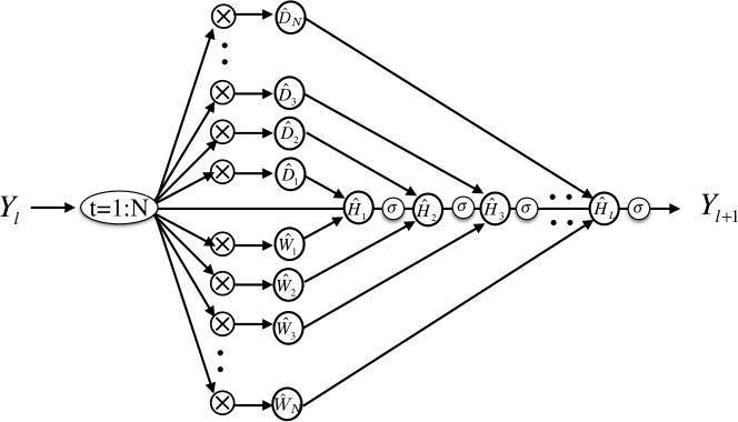
Figure 3: QUNN arcitecture: $\otimes$ represents tensor product of input with delays, oval marked by $t=1:N$ represents different values of delays, and $\sigma_{*}$ represents nonlinear activation functions at different layers.

Notice that the QUNN weight matrix changes dynamically according to Eq. (35), meaning that they evolve with the input data within the active block of length $N$. This is different from conventional definition of RNN where the weight matrix does not explicitly depend on the data, but such memory dependence is indirectly actuated through the gate construction such as the forgetting unit $f_{i}$ in LSTM (Hochreiter and Schmidhuber, 1997). The multi-layer construction of LSTM facilitates longer temporal memory as the hidden layer number $N$ increases. The depth of the hidden layers in QUNN can also be interpreted as both the order of the corresponding ODE recursion relation and the order of nonlinearity that corresponds to the stage of Runge-Kutta method, as illustrated in Fig. 3. A QUNN with $L$ hidden layers thus corresponds to a $L$-$L$-ODERNN. The the general QUNN stability can be ensured by choosing parameters in Eq. (32) and (35) according to the requirements in Theorem 1.

	QUNN	LSTM	URNN	$n$-$t$-ODERNN
memory scale	$n$	$2$	$2$	$t$
order of nonlinearity	$n$	$n$	$n$	$n$
stability	Yes	$?$	Yes	$?$
depth	$n+2$	$n$	$n$	$n$
training parameters	$O(n)$	$O(n^{2})$	$O(n^{2})$	?
origin	Schrödinger equation	Ad Hoc	Unitarity	ODE

Table 3: A top-down comparison between QUNN, LSTM, URNN and $n$-$t$-ODERNN structure.

Our top-down design of QUNN is compared with some of existing RNN architectures in Table. 3. QUNN have longer range of memory scale than both LSTM and URNN, i.e., the order of time derivatives in the corresponding ODE is higher in QUNN. This comes with a price of additional layers of embedding in RNN architecture seen in the depth difference. The data-dependent construction of QUNN weight matrices can also slow down the convergence of the training process. And certain pre-processing of data, such as calculating the autocorrelation function, is needed to give a good estimate of $N$ to make QUNN effective. But QUNN can reduce the total number of training paramters from LSTM, offering potential advantage to its training efficiency. This show cases the distinction between an ad hoc heuristic approach and physically inspired approach to RNN designs.

4 Conclusion

We propose an ODE theoretical framework for understanding RNN architectures’s order of non-linearity, length of memory scales and training stability. We apply this analysis to many existing RNN architectures, including LSTM, GRU, URNN, CW-RNN and identify the improved nonlinearity obtained by CW-RNN. Examing RNN through the eyes of ODEs help us to design new RNN architectures inspired by dynamics and stability of different ODEs and associated integration methods. As an example, we showcase the design of an RNN based on the ODEs of quantum dynamics of universal quantum computation. We show that in the case when the temporal correlation is known and the input data comes in active blocks, QUNN provides a quadratic reduction in the number of training parameters as a function of temporal correlation length than generic LSTM architectures. Our findings point to an exciting direction of developing new machine learning tools by harnessing physical knowledge of both the data and the neural network itself.

A parallel and recently published work on designing stable RNN based on ODEs with antisymmetric weight matrices by Chang et al. (2019) came to our attention after the completion of this work. There, a stable RNN architecture is proposed and implemented, which have important practical applications in improving the state-of-the-art RNN performance. In comparison, we have focused on theoretical analysis on general RNN architectures, which include the RNN design from Chang et al. (2019) as a specific case of $n$-$t$-ARNN defined in Sec.2.3 by setting $n=1$ and $t$ equals the number of connected hidden layers. And our stability proof is applicable for any RNN designed based on ODE integration methods. We aim at establishing a firm theoretical ground for a wider application of numerical toolbox in the study of Neural Networks instead of providing a ready-to-use RNN architecture. But more heuristic testing remains to be done to fully understand the practical use of tailoring temporal non-linearity of RNNs defined in this work.

	column vector	row vector	matrix	inner product	tensor product	Hadamard product
classical	$Y_{l}$	$Y_{l}^{\top}$	$W_{l}$	$Z_{l}^{\top}Y_{l}$	$Y_{l}\otimes Z_{l}$	$Y_{l}\circ Z_{l}$
quantum	${\lvert Y_{l}\rangle}$	${\langle Y_{l}\rvert}$	$\hat{W}_{l}$	${\langle Z_{l}\rvert}Y_{l}\rangle$	${\lvert Y_{l}\rangle}\otimes{\lvert Z_{l}\rangle}$	$\hat{D}[Y_{l}]{\lvert Z_{l}\rangle}$

Table 4: Comparison of the representation of linear algebra in quantum and in classical literature.

Appendix A Proof of Theorem 5.

Theorem 5. Any Boolean function from the uniform family $f:\{0,1\}^{n}\to\{0,1\}^{n}$ can be mapped to a unique fixed point of ODE evolution with its characteristic function containing polynomial in $n$ many parameters.

Proof. By definition, any polynomial-time uniform Boolean function can be represented by a deterministic Turing machine that runs in polynomial time $L_{c}$ and outputs the circuit description $\mathcal{C}_{n}$ if given $1^{n}$ as input. We only need to show that there exists a one-on-one mapping between a deterministic Turing machine of polynomial runtime and a set of ODEs that represents quantum dynamical evolution. The read and write process of a Turing machine can be mapped a rotation in the Hilbert space of input and output $\vec{r_{j}},\vec{w}_{j}\in\mathcal{H}$ at the $j$th time step as:

$$U_{j}=\vec{w_{j}}\times\vec{r}_{j}^{\top},$$ (37)

where our use of ${\lvert w_{j}\rangle}$ and the associated quantum notation henceforth is explained in Table 4. To keep track of the update in its relative location within each active block, we tensor product such matrix with a time step update matrix ${\lvert j+1\rangle}{\langle j\rvert}^{c}$ which increase the book-keeping of time $j$ by one. So the overall unitary takes the form:

$$U_{j}\otimes{\lvert j+1\rangle}{\langle j\rvert}^{c}={\lvert w_{j}\rangle}{\langle r_{j}\rvert}\otimes{\lvert j+1\rangle}{\langle j\rvert}^{c}.$$ (38)

Moreover, we add the inverse process of such Turing computing step to satisfy the Hermiticity of the overall matrix $\hat{H}_{j}$:

$$\hat{H}_{j}={\lvert w_{j}\rangle}{\langle r_{j}\rvert}\otimes{\lvert j+1\rangle}{\langle j\rvert}^{c}+{\lvert r_{j}\rangle}{\langle w_{j}\rvert}\otimes{\lvert j\rangle}{\langle j+1\rvert}^{c},$$ (39)

whose eigenvalues are purely imaginary. This consists of one step of reversible formulation of any TM computation step. Summing up all the corresponding steps for a TM that halts at step $L_{c}$, we obtain a Hermitian matrix that encode both the forward and backward computation process of a conventional TM. The ground state energy of this Hamiltonian, or the absolute value of the lowest eigenvalues, is not necessarily zero. If we like to ensure that the ground state which corresponds to the process of TM computation step is the fixed-point of the dynamical evolution, we need to add two additional term to obtain the overall Hamiltonian:

$$\hat{H}_{TM}= \sum_{j=1}^{L_{c}}\left(I\otimes{\lvert j\rangle}{\langle j\rvert}^{c}-{\lvert w_{j}\rangle}{\langle r_{j}\rvert}\otimes{\lvert j+1\rangle}{\langle j\rvert}^{c}\right.\left.-{\lvert r_{j}\rangle}{\langle w_{j}\rvert}\otimes{\lvert j\rangle}{\langle j+1\rvert}^{c}+I\times{\lvert j+1\rangle}{\langle j+1\rvert}^{c}\right)$$

whose lowest eigenvalue is exactly zero Aharonov et al. (2008).

It is shown in Aharonov et al. (2008) that the zero energy ground state of the above Hamiltonian is

$${\lvert\psi_{0}\rangle}=\frac{1}{\sqrt{L_{c}}}\sum_{j=1}^{L_{c}}{\lvert w_{j}\rangle}\otimes{\lvert j+1\rangle}$$ (40)

which is not only unique but also separated from other eigenstates in eigenvalues by a gap. Projecting the this ground state onto the clock state ${\lvert L_{c}\rangle}^{c}$ gives the output of the Turing machine that describe the desired Boolean function. Since, a polynomial runtime Turing machine can be described by polynomial sized computational tap $L_{c}$, the size of $U_{j}$ is also polynomial in the number of bits. Since the total number of terms inside this Hamiltonian equals the number of time steps $L_{c}$ in the deterministic Turing machine of the uniform Boolean functions, it is also polynomial in number of bits of the Boolean function input. Q. E. D.

References

- Aharonov et al. (2008) D. Aharonov, W. Van Dam, J. Kempe, Z. Landau, S. Lloyd, and O. Regev, Society for Industrial and Applied Mathematics (SIAM) review 50, 755 (2008).
- Arjovsky et al. (2016b) M. Arjovsky, A. Shah, and Y. Bengio, in International Conference on Machine Learning (2016b), 1120–1128.
- Alpay et al. (2016) T. Alpay, S. Heinrich, and S. Wermter, in International Conference on Artificial Neural Networks (Springer, 2016), 132–139.
- Arik (2000) S. Arik, IEEE Transactions on Circuits and Systems I: Fundamental Theory and Applications 47, 1089 (2000).
- Bengio et al. (2013) Y. Bengio, N. Boulanger-Lewandowski, and R. Pascanu, in Acoustics, Speech and Signal Processing (ICASSP), 2013 IEEE International Conference on (IEEE, 2013), 8624–8628.
- Bengio et al. (1994) Y. Bengio, P. Simard, and P. Frasconi, IEEE transactions on Neural Networks 5, 157 (1994).
- Bahdanau et al. (2015) D. Bahdanau, K. Cho, and Y. Bengio, International Conference on Learning Representations (ICLR) 2015 (2015).
- Cho et al. (2014) K. Cho, B. Van Merriënboer, C. Gulcehre, D. Bahdanau, F. Bougares, H. Schwenk, and Y. Bengio, The 2014 Conference on Empirical Methods on Natural Language Processing (EMNLP) (2014).
- Cao and Wang (2003) J. Cao and J. Wang, IEEE Transactions on Circuits and Systems I: Fundamental Theory and Applications 50, 34 (2003).
- Chen et al. (2018) T. Q. Chen, Y. Rubanova, J. Bettencourt, and D. K. Duvenaud, In Advances in Neural Information Processing Systems 31, 6572-6583 (2018).
- Chang et al. (2019) B. Chang, M. Chen, E. Haber, and Ed. Chi, arXiv preprint arXiv:1902.09689 (2019).
- Dahlquist (1979) G. Dahlquist, Signum Meeting on Numerical Ordinary Differential Equations, 1979 (1979 ).
- Graves (2013) A. Graves, arXiv preprint arXiv:1308.0850 (2013).
- Graves et al. (2014) A. Graves, G. Wayne, and I. Danihelka, arXiv preprint arXiv:1410.5401 (2014).
- Kiros et al. (2015) R. Kiros, Y. Zhu, R. R. Salakhutdinov, R. Zemel, R. Urtasun, A. Torralba, and S. Fidler, in Advances in neural information processing systems (2015), 3294–3302.
- Pascanu et al. (2013) R. Pascanu, T. Mikolov, and Y. Bengio, in International Conference on Machine Learning (2013), 1310–1318.
- Hochreiter and Schmidhuber (1997) S. Hochreiter and J. Schmidhuber, Neural Computation 9, 1735 (1997).
- Koutnik et al. (2014) J. Koutnik, K. Greff, F. Gomez, and J. Schmidhuber, arXiv preprint arXiv:1402.3511 (2014).
- Jing et al. (2016) L. Jing, Y. Shen, T. Dubček, J. Peurifoy, S. Skirlo, Y. LeCun, M. Tegmark, and M. Soljačić, Neural Computation, 31, 765 (2016).
- Jaeger et al. (2007) H. Jaeger, M. Lukoševičius, D. Popovici, and U. Siewert, Neural Networks 20, 335 (2007).
- Jozefowicz et al. (2015) R. Jozefowicz, W. Zaremba, and I. Sutskever, in International Conference on Machine Learning (2015), 2342–2350.
- Karpathy et al. (2015) A. Karpathy, J. Johnson, and L. Fei-Fei, International Conference on Learning Representations (ICLR) Workshops (2015).
- Greff et al. (2017) K. Greff, R. K. Srivastava, J. Koutník, B. R. Steunebrink, and J. Schmidhuber, IEEE transactions on Neural Networks and learning systems 28, 2222 (2017).
- Hochreiter et al. (2001) S. Hochreiter, Y. Bengio, P. Frasconi, J. Schmidhuber, et al., Gradient flow in recurrent nets: the difficulty of learning long-term dependencies (2001).
- Schmidhuber (2015) J. Schmidhuber, Neural Networks 61, 85 (2015).
- Jin et al. (1994) L. Jin, P. N. Nikiforuk, and M. M. Gupta, IEEE Transactions on Neural Networks 5, 954 (1994).
- Mandic et al. (2001) D. P. Mandic, J. A. Chambers, et al., Recurrent Neural Networks for prediction: learning algorithms, architectures and stability (Wiley Online Library, 2001).
- Haber and Ruthotto (2017) E. Haber and L. Ruthotto, Inverse Problems 34, 014004 (2017).
- Haykin (1994) S. Haykin, Neural Networks: a comprehensive foundation,Prentice Hall PTR, (1994).
- Kosmatopoulos et al. (1995) E. B. Kosmatopoulos, M. M. Polycarpou, M. A. Christodoulou, and P. A. Ioannou, IEEE transactions on Neural Networks 6, 422 (1995).
- Mhaskar and Poggio (2016) H. N. Mhaskar and T. Poggio, Analysis and Applications 14, 829 (2016).
- Feynman (1986) R. P. Feynman, Foundations of physics 16, 507 (1986).
- Kitaev et al. (2002) A. Y. Kitaev, A. Shen, and M. N. Vyalyi, Classical and quantum computation, 47 (American Mathematical Soc., 2002).
- McKague et al. (2009) M. McKague, M. Mosca, and N. Gisin, Phys. Rev. Lett. 102, 020505 (2009).
- Lu et al. (2017) Y. Lu, A. Zhong,Q. LI, B. Dong, arXiv preprint arXiv:1710.10121, (2017)
- Ruthotto et al. (2018) L. Ruthotto, E. Haber, arXiv preprint arXiv:1804.04272, (2018)
- Runge (1895) C. Runge, Mathematische Annalen 46, 167-178 (1895).
- Kutta (1901) C. Runge, Beitrag zur näherungweisen Integration totaler Differentialgleichungen (1901).
- Wikipedia (2019) Wikipedia contributors, Long short-term memory .
- Wermter et al. (1999) S. Wermter, C. Panchev, and G. Arevian, in Proceedings of the 16th National Conference on Artificial Intelligence (AAAI-99), 93–98(1999).
- Rezende and Mohamed (2015) D. J. Rezende, and S. Mohamed, Proceedings of the 32Nd International Conference on International Conference on Machine Learning 371, 1530–1538 (2015).
- Sutskever et al. (2014) I. Sutskever, O. Vinyals, and Q. V. Le, in Advances in neural information processing systems, 3104–3112 (2014).
- Srivastava et al. (2015) N. Srivastava, E. Mansimov, and R. Salakhudinov, in International conference on machine learning , 843–852(2015).
- Spijker (1980) M. N. Spijker W. H. Hundsdorfer, Numerische Mathematik 50, 319 (1980).
- Zhang and Zeng (2018) F. Zhang and Z. Zeng, Neural Networks 97, 116 (2018).