Classicalization by phase space measurements

Abstract

This article provides an accessible illustration of the measurement approach to the study of the quantum-classical transition suitable for beginning graduate students. As an example, we apply it to a quantum system with a general quadratic Hamiltonian and obtain the exact solution of the dynamics for an arbitrary measurement strength.

Keywords: quantum-classical transition, measurement master equation, phase space methods

1 Introduction

The study of the quantum-classical transition is an active field of research that has provided important insights into the foundations of quantum theory and plays a prominent role in the development of quantum technologies [1].

Some of its achievements have been obtained through the measurement approach, which consists in using the framework of generalized measurements [2] to model the dynamics of an open quantum system, i.e. a quantum system in interaction with a large number of quantum degrees of freedom, which are collectively called environment. This has been used, for example, to develop a quantitative assessment of the macroscopic character of a superposition state based on the experimental observation of quantum effects [3].

The concepts and methods used in this field are usually not familiar to beginning graduate students. However, some of them have been discussed in a pedagogical way in recent years [4, 5, 6, 7]. The main contribution of this article is to present an accessible illustration of the measurement approach applied to an analytically tractable model for the classicalization of a quantum system described by a general quadratic Hamiltonian. This should be useful for instructors with an interest in introducing graduate students to current research topics in quantum mechanics.

The manuscript is organized as follows. In section 2, the Heisenberg–Dirac formulation of quantum mechanics is briefly discussed, with a focus on physical dimensions and algebraic considerations. These two aspects will play an important role throughout the article. We remark that the use of algebraic methods in quantum mechanics has lead to a deeper understanding of nature, while also offering an elegant and powerful framework to study a wide variety of systems [8, 9]. Section 3 contains a brief account of the phase space formulation of quantum mechanics, which allows one to establish a connection with classical mechanics. In section 4 generalized measurements are defined and it is shown how to construct a dynamical equation for the state of a system subject to such measurement. Section 5 contains an example of measurement-induced classicalization. In particular, we consider an imprecise, simultaneous measurement of two canonically conjugate observables of a quantum harmonic oscillator, which leads to the decay of all the coherences in a superposition state.

2 Heisenberg–Dirac quantum mechanics

In analogy to classical Hamiltonian mechanics, the observable quantities of an elementary quantum system are described by operator-valued functions of two self-adjoint operators $\mathsf{Q}=\mathsf{Q}^{\dagger},\mathsf{P}=\mathsf{P}^{\dagger}$ satisfying the canonical commutation relation

$$[\mathsf{Q},\mathsf{P}]=i\hbar\mathsf{I}.$$ (2.1)

The operators $\mathsf{Q}$, $\mathsf{P}$, and $\mathsf{I}$ (identity) are the canonical basis of the Heisenberg Lie algebra $\mathfrak{h}(3)$ [10]. It is customary to choose units in which $\hbar=1$, but this makes it difficult to verify that an equation has the correct dimensions. For economy of notation it is preferable to use the dimensionless basis of $\mathfrak{h}(3)$ given by [11]

$$\mathsf{a}=\frac{1}{\sqrt{2}}\left(\frac{\mathsf{Q}}{\lambda}+\frac{i}{\hbar}\mathsf{P}\lambda\right),\quad\mathsf{a}^{\dagger}=\frac{1}{\sqrt{2}}\left(\frac{\mathsf{Q}}{\lambda}-\frac{i}{\hbar}\mathsf{P}\lambda\right),\quad\mathsf{I},$$ (2.2)

where $\lambda$ has the same dimensions as $\mathsf{Q}$, $\mathsf{P}$ has dimensions of $\hbar/\lambda$ and $\mathsf{a},\mathsf{a}^{\dagger}$ satisfy the commutation relation

$$[\mathsf{a},\mathsf{a}^{\dagger}]=\mathsf{I}.$$ (2.3)

Correspondingly, the observable quantities of the system can be expressed as operator-valued functions of $\mathsf{a}$ and $\mathsf{a}^{\dagger}$. For example, the operator $\mathsf{N}=\mathsf{a}^{\dagger}\mathsf{a}$ together with the operators $\mathsf{a}$, $\mathsf{a}^{\dagger}$, $\mathsf{I}$ generates the Lie algebra $\mathfrak{h}(4)$. From the commutators

$$[\mathsf{a},\mathsf{N}]=\mathsf{a},\quad[\mathsf{a}^{\dagger},\mathsf{N}]=-\mathsf{a}^{\dagger}$$ (2.4)

follows [10] that $\mathsf{a}$ and $\mathsf{a}^{\dagger}$ are ladder operators with respect to the eigenvectors $|n\rangle=(\mathsf{a}^{\dagger})^{n}|0\rangle/\sqrt{n!}$ of $\mathsf{N}$:

$$\mathsf{a}\,|n\rangle=\sqrt{n}\,|n-1\rangle,\quad\mathsf{a}^{\dagger}|n\rangle=\sqrt{n+1}\,|n+1\rangle,$$ (2.5)

and we require that $\mathsf{a}\,|0\rangle=0$ (because the energy of a quantum system must be bounded from below). These eigenvectors form a complete and orthonormal ($\langle n|m\rangle=\delta_{nm}$) set that spans a Hilbert space $\mathcal{H}$, in which one can represent the state of a system described by $\mathfrak{h}(4)$, e.g. the quantum harmonic oscillator.

An eigenvector $|\alpha\rangle$ of the operator $\mathsf{a}$ is called a coherent state. The corresponding eigenvalue, $\alpha$, is a complex number, since this operator is not self-adjoint. In the basis $|n\rangle$, a coherent state is expressed as [10]

$$|\alpha\rangle=e^{-\frac{1}{2}|\alpha|^{2}}\sum_{n=0}^{\infty}\frac{\alpha^{n}}{\sqrt{n!}}|n\rangle.$$ (2.6)

These states play a fundamental role in the study of the quantum-classical transition [12]. This becomes apparent with the use of phase space methods, which will be discussed in the following section.

3 Quantum mechanics in phase space

Quantum mechanics can also be formulated in terms of unitary operators, i.e. operators that satisfy $\mathsf{O}\mathsf{O}^{\dagger}=\mathsf{O}^{\dagger}\mathsf{O}=\mathsf{I}$. In this framework, the operators associated with $\mathsf{Q}$ and $\mathsf{P}$ are [13]

$$\mathsf{U}(a)=e^{\frac{i}{\hbar}a\mathsf{Q}},\quad\mathsf{V}(b)=e^{\frac{i}{\hbar}b\mathsf{P}}.$$ (3.1)

Since the argument of the exponential function must be dimensionless, $a$ has the dimensions of $\mathsf{P}$ and $b$ has the dimensions of $\mathsf{Q}$. The above operators are a special case of the Weyl operators (or displacement operators)

$$\mathsf{D}(a,b)=e^{\frac{i}{\hbar}(a\,\mathsf{Q}\,+\,b\,\mathsf{P})},$$ (3.2)

which satisfy the canonical commutation relations in Weyl (or integral) form [13]

$$\mathsf{D}(a_{1},b_{1})\,\mathsf{D}(a_{2},b_{2})=e^{-\frac{i}{2\hbar}[a_{1}b_{2}-a_{2}b_{1}]}\mathsf{D}(a_{1}+a_{2},b_{1}+b_{2}).$$ (3.3)

In terms of the operators $\mathsf{a}$ and $\mathsf{a}^{\dagger}$, the displacement operator is given by [10]

$$\mathsf{D}(\alpha)=e^{\,\alpha\,\mathsf{a}^{\dagger}-\,\alpha^{\ast}\mathsf{a}}=e^{-\frac{1}{2}|\alpha|^{2}}e^{\alpha\,\mathsf{a}^{\dagger}}e^{-\alpha^{\ast}\mathsf{a}}.$$ (3.4)

The coherent states can also be defined as displaced ground states $|\alpha\rangle:=\mathsf{D}(\alpha)|0\rangle$, as can be seen by comparing this expression with (2.6).

The operators acting on a representation space (such as the Hilbert space spanned by the vectors $|n\rangle$) belong to a Hilbert space called Liouville space, in which the scalar product is given by $\langle\mathsf{A}|\mathsf{B}\rangle=\mathrm{Tr}(\mathsf{A}^{\dagger}\mathsf{B})$. The set of displacement operators $\mathsf{D}(\alpha)$ forms a delta-orthogonal basis of this space: $\langle\mathsf{D}(\alpha)|\mathsf{D}(\beta)\rangle=\pi\delta^{(2)}(\alpha-\beta)$.

In this basis, the density operator (or state operator) $\rho$ of a quantum system is described by the Weyl characteristic function (also called ambiguity function) [14]

$$\chi(\eta,\eta^{\ast})=\mathrm{Tr}[\rho\,\mathsf{D}(\eta)],$$ (3.5)

which will figure prominently in section 5. The following Fourier transform of $\chi(\eta,\eta^{\ast})$ yields the Wigner function [14]:

$$W(\xi,\xi^{\ast})=\frac{1}{\pi^{2}}\int\mathrm{d}^{2}\eta\,\chi(\eta,\eta^{\ast})\,e^{\,\xi\eta^{\ast}-\,\xi^{\ast}\eta},\quad\mathrm{d}^{2}\eta=\mathrm{d}\mathrm{Re}(\eta)\,\mathrm{d}\mathrm{Im}(\eta),$$ (3.6)

which can also be defined as $W(\xi,\xi^{\ast})=\mathrm{Tr}[\rho\,\mathsf{\Pi}(\xi)]$, where

$$\mathsf{\Pi(\xi)}=\frac{2}{\pi}\exp{\bigl{[}i\pi(\mathsf{a}^{\dagger}-\xi^{\ast})(\mathsf{a}-\xi)\bigr{]}}$$ (3.7)

is the Wigner operator (or displaced parity operator) [15], which is self-adjoint and therefore is an observable, unlike the displacement operator. This implies that the Wigner function is real, whereas the characteristic function is complex. The geometrical interpretation of these functions is discussed in [16]. For the experimental determination of the Wigner function we refer the reader to [17].

We remark that it is customary to denote the operators $\mathsf{D}$ and $\mathsf{\Pi}$ with a single complex argument even though $\chi$ and $W$ are functions of two complex variables. This mapping of operators to functions, also known as a mapping from $q$-numbers to $c$-numbers, is very useful in the study of the quantum-classical transition, as will be shown in section 5. For a thorough discussion of mappings of this kind we refer the reader to [18, 19].

For a coherent state, $W$ is Gaussian, which can easily be seen using (3.4)–(3.6) together with the fact that a coherent state is an eigenvector of $\mathsf{a}$. However, for a so-called cat state

$$|\psi\rangle=\mathcal{N}^{1/2}(|\alpha\rangle+|-\alpha\rangle),\quad\mathcal{N}^{-1}=2(1+e^{-2|\alpha|^{2}}),$$ (3.8)

$W$ takes negative values:

$$W(\xi,\xi^{\ast})=\frac{2\,\mathcal{N}}{\pi}\Bigl{[}e^{-2|\xi-\alpha|^{2}}+\,e^{-2|\xi+\alpha|^{2}}+\,2\,e^{-2|\xi|^{2}}\cos{(4\,\mathrm{Im}(\alpha^{\ast}\xi))}\Bigr{]}.$$ (3.9)

This is a signature of a non-classical state [20]. Moreover, it can be proven that the only positive-definite Wigner functions describing pure states are Gaussian [21]. This is one reason why coherent states are considered the most classical quantum states.

It can be shown [20] that for a Hamiltonian with a general quadratic potential $\mathsf{V}(\mathsf{q})=a\,\mathsf{q}^{2}+b\,\mathsf{q}+c$, the evolution of the Wigner function is given by the classical Liouville equation for a probability distribution in phase space:

$$\frac{\partial}{\partial t}W(q,p,t)=\frac{\partial H}{\partial q}\frac{\partial W}{\partial p}-\frac{\partial H}{\partial p}\frac{\partial W}{\partial q}.$$ (3.10)

However, this does not represent classical behavior unless the Wigner function is positive. For this reason, $W$ is called a quasi-probability phase space distribution. Moreover, as a consequence of Heisenberg’s uncertainty principle, the Wigner function cannot have a width smaller than the size of a Planck cell: $\Delta q\Delta p\geq\hbar$ [20]. Therefore, quantum mechanics introduces a coarse-graining in phase space.

One reason why quasi-probability distributions are useful is that they enable calculating quantum-mechanical expectation values similarly to averages in classical statistical mechanics. In particular, distributions belonging to the Cohen class [22], which includes the Wigner function, have the property that integrating them with respect to one canonical variable yields the probability distribution of the canonically conjugate variable.

In the literature, it is common to describe the transition to classical behavior as “taking the limit $\hbar\rightarrow 0$”. However, this characterization is misleading, since $\hbar$ is a constant of nature and it cannot be made arbitrarily small. What is meant by this statement is that one may form a dimensionless parameter involving $\hbar$ and other physical quantities, such that when this parameter is made arbitrarily small, a quantum equation reduces to a classical one (e.g. the Liouville equation above). This shows again the importance of dimensional considerations in quantum mechanics. We remark that this limiting procedure does not lead to the vanishing of negative regions in the Wigner function.

4 Quantum measurements and the measurement master equation

4.1 Measurement in quantum mechanics

In the axiomatization of quantum mechanics carried out by von Neumann [23], given an observable with a discrete spectrum $\mathsf{O}=\sum_{n}\lambda_{n}|\lambda_{n}\rangle\langle\lambda_{n}|$, the probability that a measurement of $\mathsf{O}$ yields the result $\lambda_{n}$ is

$$\mathrm{Prob}(\lambda_{n})=\mathrm{Tr}[\rho\,|\lambda_{n}\rangle\langle\lambda_{n}|],$$ (4.1)

and the state of the system after the measurement is $\rho=|\lambda_{n}\rangle\langle\lambda_{n}|$. If the measurement result is not known, the system is described by the mixed state

$$\rho=\sum_{n}\mathrm{Prob}(\lambda_{n})|\lambda_{n}\rangle\langle\lambda_{n}|.$$ (4.2)

Instead of associating a projector with each measurement result $n$, in general one may associate a positive operator $\pi_{n}$ with it. These operators form a positive-operator-valued measure (POVM) [2] and must be such that $\sum_{n}\pi_{n}=\mathsf{I}$. Moreover, each operator $\pi_{n}$ may be decomposed in terms of pairs ($\mathsf{A}_{k},\mathsf{A}_{k}^{\dagger}$) of operators:

$$\pi_{n}=\sum_{k}\mathsf{A}_{nk}^{\dagger}\mathsf{A}_{nk}.$$ (4.3)

In this framework, the probability that a measurement yields the result $n$ is $\mathrm{Prob}(n)=\mathrm{Tr}[\rho\,\pi_{n}]$ and the state of the system after the measurement is $\rho=(\mathrm{Tr}[\rho\,\pi_{n}])^{-1}\sum_{k}\mathsf{A}_{nk}\,\rho\,\mathsf{A}_{nk}^{\dagger}$. If the measurement result is not known, the state of a system after performing a generalized measurement is given by

$$\rho=\sum_{n}\mathrm{Prob}(n)\frac{\sum_{k}\mathsf{A}_{nk}\,\rho\,\mathsf{A}_{nk}^{\dagger}}{\mathrm{Tr}[\rho\,\pi_{n}]}=\sum_{n,k}\mathsf{A}_{nk}\,\rho\,\mathsf{A}_{nk}^{\dagger}.$$ (4.4)

We remark that this formalism is quite general and when the measurement result can take any real or complex value the sums are replaced by corresponding integrals.

4.2 Measurement master equation

The dynamics of the state operator of an open quantum system is described under certain approximations by the Lindblad–Gorini–Kossakowski–Sudarshan master equation:

$$\frac{\partial\rho}{\partial t}=-\frac{i}{\hbar}[\mathsf{H},\rho]+\frac{1}{2}\sum_{j=1}^{d}\kappa_{j}\Bigl{(}2\,\mathsf{R}_{j}\rho\mathsf{R}_{j}^{\dagger}-\mathsf{R}_{j}^{\dagger}\mathsf{R}_{j}\rho-\rho\,\mathsf{R}_{j}^{\dagger}\mathsf{R}_{j}\Bigr{)},$$ (4.5)

where $\mathsf{H}$ is a self-adjoint operator with dimension of energy, $\mathsf{R}_{j}$ are arbitrary dimensionless operators and $\kappa_{j}$ are non-negative real numbers with dimension of frequency. Here we are only interested in using this equation and refer the reader to [24] for an in depth discussion of its derivation and the physical considerations behind it.

The change in the state of a system subject to a generalized measurement can be modeled as a Poisson process with rate $\gamma$ [25], as follows. We assume that in a short time interval $\Delta t$ the probability that a measurement occurs is $\gamma\Delta t$. If a measurement occurs, then the state at the time $t+\Delta t$ will be given by (4.4). Otherwise, the state at this time results from the unitary evolution of the system, given by the first term in the right-hand side of (4.5). To first order in $\Delta t$, the state of a system subject to this stochastic process is described at time $t+\Delta t$ by

$$\rho(t+\Delta t)=(1-\gamma\Delta t)\rho(t)-\frac{i}{\hbar}[\mathsf{H},\rho(t)]\Delta t+\gamma\Delta t\sum_{n,k}\mathsf{A}_{nk}\,\rho(t)\,\mathsf{A}_{nk}^{\dagger}.$$ (4.6)

In the limit $\Delta t\rightarrow 0$ one obtains the measurement master equation [26]

$$\frac{\partial\rho}{\partial t}=-\frac{i}{\hbar}[\mathsf{H},\rho]+\gamma\Biggl{[}\sum_{n,k}\mathsf{A}_{nk}\,\rho\,\mathsf{A}_{nk}^{\dagger}-\rho\Biggr{]},$$ (4.7)

which can be shown to be of the type (4.5).

5 Classicalization of systems with a quadratic Hamiltonian

A general quadratic Hamiltonian in the basis $\mathsf{Q}$, $\mathsf{P}$ is of the form:

$$\mathsf{H}=c_{1}\mathsf{Q}^{2}+c_{2}\mathsf{P}^{2}+c_{3}(\mathsf{Q}\mathsf{P}+\mathsf{P}\mathsf{Q})+c_{4}\mathsf{Q}+c_{5}\mathsf{P},\quad c_{i}\in\mathbb{R}.$$ (5.1)

The corresponding expression in a dimensionless basis analogous to (2.2) is:

$$\mathsf{H}=z_{1}\mathsf{b}^{\dagger}\mathsf{b}+z_{2}\mathsf{b}^{2}+z_{2}^{\ast}(\mathsf{b}^{\dagger})^{2}+z_{3}\mathsf{b}+z_{3}^{\ast}\mathsf{b}^{\dagger},\quad z_{1}\in\mathbb{R},\quad z_{2},z_{3}\in\mathbb{C}.$$ (5.2)

Using a canonical transformation (see A) one obtains from (5.2) the harmonic oscillator-like Hamiltonian ($z_{0}=(z_{1}^{2}-4|z_{2}|^{2})^{1/2}$, $\phi=\mathrm{Arg}(z_{2})$):

$$\mathsf{H}=z_{0}\,\mathsf{a}^{\dagger}\mathsf{a}+c\,\mathsf{I},$$ (5.3)

with

$$\mathsf{b}=\biggl{[}\frac{1}{2}\frac{z_{1}+z_{0}}{z_{0}}\biggr{]}^{1/2}e^{i\phi/2}\,\mathsf{a}+\biggl{[}\frac{1}{2}\frac{z_{1}-z_{0}}{z_{0}}\biggr{]}^{1/2}e^{i\phi/2}\,\mathsf{a}^{\dagger}+\frac{2z_{2}z_{3}^{\ast}-z_{1}z_{3}}{z_{0}^{2}}\mathsf{I}$$

and

$$c=\frac{1}{2}(z_{0}-z_{1})+\frac{1}{z_{0}^{2}}\left(z_{2}(z_{3}^{\ast})^{2}+z_{2}^{\ast}z_{3}^{2}-z_{1}|z_{3}|^{2}\right).$$

We note that the constant $c$ in the Hamiltonian does not affect the dynamics and, therefore, in this basis the system behaves like a harmonic oscillator with ground-state energy zero. This is a demonstration of the usefulness of algebraic methods in quantum mechanics. In the following we will set $z_{0}=\hbar\,\omega$.

5.1 Simultaneous imprecise measurement of the quadratures of the harmonic oscillator

For the quantum harmonic oscillator (5.3) one can define the dimensionless self-adjoint quadrature operators:

$$\mathsf{X}=\frac{1}{2}(\mathsf{a}+\mathsf{a}^{\dagger}),\quad\mathsf{Y}=\frac{1}{2i}(\mathsf{a}-\mathsf{a}^{\dagger}),\quad[\mathsf{X},\mathsf{Y}]=\frac{i}{2}.$$ (5.4)

For any state of the harmonic oscillator, the Heisenberg uncertainty product is given by $\Delta\mathsf{X}\,\Delta\mathsf{Y}\geq 1/4$, with $\Delta\mathsf{O}=(\langle\mathsf{O}^{2}\rangle-\langle\mathsf{O}\rangle^{2})^{1/2}$. States that satisfy the equality are called minimum-uncertainty states. For example, coherent states have this property: $\Delta\mathsf{X}=\Delta\mathsf{Y}=\frac{1}{2}$. This is another reason why coherent states are considered the most classical quantum states. The eigenvalues of $\mathsf{X}$ and $\mathsf{Y}$ are the real and imaginary parts of the amplitude $\alpha=\alpha_{x}+i\alpha_{y}$. A measurement of $\alpha$ can be described using the formalism of generalized measurements of section 4, as follows.

Given a positive operator with unit trace $\Psi$, one can define the operators [27]:

$$\pi_{\alpha}=\frac{1}{\pi}\mathsf{D}(\alpha)\Psi\mathsf{D}^{\dagger}(\alpha),\quad\int\mathrm{d}^{2}\alpha\,\pi_{\alpha}=\mathsf{I}.$$ (5.5)

The probability density of obtaining the result $\alpha$ is $\mathrm{Prob}(\alpha)=\mathrm{Tr}[\pi_{\alpha}\,\rho]$, and its moments are given by

$$M_{ij}=\int\mathrm{d}^{2}\alpha\,\mathrm{Prob}(\alpha)\,\alpha_{x}^{i}\,\alpha_{y}^{j},\quad\mathrm{d}^{2}\alpha=\mathrm{d}\alpha_{x}\,\mathrm{d}\alpha_{y}.$$ (5.6)

The expectation values of $\alpha_{x}$ and $\alpha_{y}$ are given by

$$\langle\alpha_{x}\rangle = M_{10}=\langle\mathsf{X}\rangle_{\rho}-\langle\mathsf{X}\rangle_{\Psi},$$

$$\langle\alpha_{y}\rangle = M_{01}=\langle\mathsf{Y}\rangle_{\rho}-\langle\mathsf{Y}\rangle_{\Psi},$$ (5.7)

so in order for the measurement to be unbiased, the expectation values with respect to $\Psi$ must be zero. The second-order moments give the mean square uncertainty for the simultaneous measurement of $\alpha_{x}$ and $\alpha_{y}$:

$$\langle(\Delta\alpha_{x})^{2}\rangle = M_{20}-(M_{10})^{2}=\langle\mathsf{X}^{2}\rangle_{\rho}+\langle\mathsf{X}^{2}\rangle_{\Psi},$$

$$\langle(\Delta\alpha_{y})^{2}\rangle = M_{02}-(M_{01})^{2}=\langle\mathsf{Y}^{2}\rangle_{\rho}+\langle\mathsf{Y}^{2}\rangle_{\Psi},$$ (5.8)

which shows that the measurement contributes (classical noise) to the uncertainty (quantum noise) of the measured state. Therefore, it is an imprecise, simultaneous measurement of two non-commuting observables. In the following we will show that this interaction between the harmonic oscillator and the system described by $\Psi$ leads to classicalization of the former.

5.2 Measurement-induced classicalization

From the theory of generalized measurements in section 4, the operators (5.5) can be written as:

$$\pi_{\alpha}=\mathsf{A}^{\dagger}_{\alpha}\mathsf{A}_{\alpha},\quad\mathsf{A}_{\alpha}=\frac{1}{\sqrt{\pi}}\,\mathsf{D}(\alpha)\Psi^{1/2}\mathsf{D}^{\dagger}(\alpha).$$ (5.9)

In turn, $\mathsf{A}_{\alpha}$ can be written in the basis of displacement operators:

$$\mathsf{A}_{\alpha}=\int\mathrm{d}^{2}\beta\,\mathsf{D}(\beta)\mathrm{Tr}[\mathsf{D}^{\dagger}(\beta)\mathsf{A}_{\alpha}]=\frac{1}{\sqrt{\pi}}\int\mathrm{d}^{2}\beta\,\mathsf{D}(\beta)\,e^{\,\beta^{\ast}\alpha\,-\,\alpha^{\ast}\beta}\chi^{\ast}_{\Psi^{1/2}}(\beta),$$ (5.10)

where we used the cyclic property of the trace, the definition (3.5) and the identity

$$\mathsf{D}^{\dagger}(\xi)\mathsf{D}(\zeta)\mathsf{D}(\xi)=\mathsf{D}(\zeta)\exp{(\xi^{\ast}\zeta-\zeta^{\ast}\xi)}.$$ (5.11)

In this representation,

$$\int\mathrm{d}^{2}\alpha\,\mathsf{A}_{\alpha}\,\rho\,\mathsf{A}_{\alpha}^{\dagger}=\pi\int\mathrm{d}^{2}\gamma\,\mathsf{D}(\gamma)\,\rho\,\mathsf{D}^{\dagger}(\gamma)\,|\chi_{\Psi^{1/2}}(\gamma)|^{2},$$ (5.12)

where we used the identity

$$\delta^{(2)}(\beta\,-\,\gamma)=\frac{1}{\pi^{2}}\int_{-\infty}^{\infty}\mathrm{d}^{2}\alpha\exp[\alpha\beta^{*}-\alpha^{*}\beta]\exp[\alpha^{*}\gamma-\alpha\gamma^{*}].$$ (5.13)

Defining the even, positive-definite function $g(|\alpha|):=\mathcal{N}\,|\chi_{\Psi^{1/2}}(\alpha)|^{2}$, where $\mathcal{N}$ is a normalization constant, we finally arrive at the master equation corresponding to the measurement described above:

$$\frac{\partial\rho}{\partial t}=-\frac{i}{\hbar}[\mathsf{H},\rho]+\gamma\int\mathrm{d}^{2}\alpha\,g(|\alpha|)[\mathsf{D}(\alpha)\,\rho\,\mathsf{D}^{\dagger}(\alpha)-\rho],$$ (5.14)

where $\mathsf{H}$ is defined in (5.3). The integral term can be interpreted as describing phase space “kicks” occurring with rate $\gamma$ and with a $g$-distributed strength $\alpha$.

Taking the trace of (5.14) multiplied with $\mathsf{D}(\eta)$ yields the following mapping from operators to functions:

$$\mathsf{a}^{\dagger}\mathsf{a}\,\rho\rightarrow\biggl{(}-\frac{\partial}{\partial\eta}\frac{\partial}{\partial\eta^{\ast}}+\eta^{\ast}\frac{\partial}{\partial\eta^{\ast}}\biggr{)}\chi_{\rho}(\eta,\eta^{\ast},t),$$

$$\rho\,\mathsf{a}^{\dagger}\mathsf{a}\rightarrow\biggl{(}-\frac{\partial}{\partial\eta}\frac{\partial}{\partial\eta^{\ast}}+\eta\frac{\partial}{\partial\eta}\biggr{)}\chi_{\rho}(\eta,\eta^{\ast},t),$$

$$\int\mathrm{d}^{2}\alpha\,g(|\alpha|)\,\mathsf{D}(\alpha)\,\rho\,\mathsf{D}^{\dagger}(\alpha)\rightarrow\chi_{\rho}(\eta,\eta^{\ast},t)\,\chi_{g}(|\eta|),$$ (5.15)

and the corresponding dynamic equation for the characteristic function:

$$\biggl{(}\frac{\partial}{\partial t}+i\omega[\eta^{\ast}\partial_{\eta^{\ast}}-\eta\partial_{\eta}]+\gamma[1-\chi_{g}(|\eta|)]\biggr{)}\chi_{\rho}(\eta,\eta^{\ast},t)=0.$$ (5.16)

Introducing the function $\tilde{\chi}_{\rho}(\eta,\eta^{\ast},t)=\chi_{\rho}(\eta e^{i\omega t},\eta^{\ast}e^{-i\omega t}t)$, the equality of the total differentials yields:

$$\frac{\partial\tilde{\chi}_{\rho}}{\partial t}=i\omega\eta\frac{\partial\chi_{\rho}}{\partial\eta}-i\omega\eta^{\ast}\frac{\partial\chi_{\rho}}{\partial\eta^{\ast}}+\frac{\partial\chi_{\rho}}{\partial t},$$ (5.17)

from which one obtains the equation of motion for the characteristic function of the state in a frame rotating with frequency $\omega$:

$$\frac{\partial}{\partial t}\tilde{\chi}_{\rho}(\eta,\eta^{\ast},t)=-\,\gamma[1-\chi_{g}(|\eta|)]\,\tilde{\chi}_{\rho}(\eta,\eta^{\ast},t),$$ (5.18)

which in the non-rotating frame has the solution:

$$\chi_{\rho}(\eta,\eta^{\ast},t)=\chi_{0}(\eta e^{i\omega t},\eta^{\ast}e^{-i\omega t})\exp\{-\,\gamma t[1-\chi_{g}(|\eta|)]\}.$$ (5.19)

For economy of notation, in the following we omit the second argument of $\chi_{\rho}$. We recognize the exponential term as the characteristic function of a compound Poisson process with rate $\gamma t$ and jump-size distribution $g$ [25]. Since $\chi_{g}$ is the characteristic function of a probability distribution, it satisfies $\chi_{g}(0)=1$ and in the limit $|\eta|\rightarrow\infty$ it vanishes for all $t$: $\chi_{g}(|\eta|)\rightarrow 0$. Therefore, at any time the exponential term is an even function that asymptotically decays in phase space towards the plane $f(\eta)=e^{-\gamma t}$, which in turn decays with time towards zero.

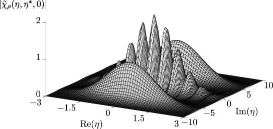
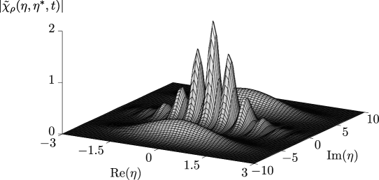
Figure 1: Top: $|\chi(\eta,0)|$ for the cat state (3.9) with $\alpha=3i$. Bottom: Snapshot of $|\chi(\eta,t)|$ at $\gamma t=1$ for the cat state subject to an imperfect, simultaneous measurement of the quadratures assuming $g$ to be a Gaussian distribution. The strong damping of the outer peaks indicates that the measurement is classicalizing the state.

Let us assume that $\chi_{0}$ corresponds to the cat state (3.9). Since $\chi_{\rho}$ is a complex function related to the Wigner function through a Fourier transform, we can interpret $|\chi_{\rho}(\eta,t)|$ as a phase space Fourier spectrum [28]. For $t=0$, it is shown in the top panel in figure 1. The central, structured peak corresponds to the low frequencies of the Wigner function, whereas the two outer peaks correspond to the high frequencies, which are associated to the non-classical character of the state.

A snapshot of the dynamics given by (5.18) is shown in the bottom panel for $\gamma t=1$. For illustration purposes, the distribution $g$ is assumed to be Gaussian. The noticeable suppression of the outer peaks is due to the “filtering” effect of the measurement, described by the decaying exponential term in (5.19). Moreover, repeating the above analysis for a coherent state reveals that it will be broadened, as expected from (5.1). Therefore, it is clear that the measurement drives a superposition state of the harmonic oscillator towards a mixture of Gaussian states, which corresponds to a classical phase space function.

It is interesting to consider the case of very frequent and very small phase-space kicks, which amounts to assuming that $\gamma\rightarrow\infty$ and that the second moments of the distribution $g$ are much larger than the higher moments, but their product with $\gamma$ remains finite. Performing a series expansion of the displacement operator to second order in $\eta$:

$$\mathsf{D}(\eta)\approx\mathsf{I}+\eta\mathsf{a}^{\dagger}-\eta^{\ast}\mathsf{a}+\frac{1}{2}(\eta\mathsf{a}^{\dagger}-\eta^{\ast}\mathsf{a})(\eta\mathsf{a}^{\dagger}-\eta^{\ast}\mathsf{a}),$$ (5.20)

one obtains from (5.14) a master equation describing diffusion in phase space [29]:

$$\frac{\partial\rho}{\partial t}=-i\omega[\mathsf{a}^{\dagger}\mathsf{a},\rho]-\kappa(-2\,\mathsf{a}\,\rho\,\mathsf{a}^{\dagger}+\mathsf{a}^{\dagger}\mathsf{a}\,\rho+\rho\,\mathsf{a}^{\dagger}\mathsf{a}-2\,\mathsf{a}^{\dagger}\rho\,\mathsf{a}+\mathsf{a}\,\mathsf{a}^{\dagger}\rho+\rho\,\mathsf{a}\,\mathsf{a}^{\dagger}).$$ (5.21)

In fact, one can describe this dynamics in terms of the Brownian motion of the state vector of the system in Hilbert space [30]. This and other master equations describing Gaussian dynamics are thoroughly discussed in [11]. It is interesting to note that under this kind of evolution, the Wigner function becomes positive everywhere in a finite time [31], in contrast to the example discussed here.

6 Conclusions

The model presented in section 5 illustrates the measurement approach to the classicalization of a quantum system by means of a master equation that can be solved exactly for an arbitrary measurement strength (“kick” size). Throughout the article, we aimed at keeping the presentation general and, at the same time, accessible. This should enable newcomers to the field to apply the measurement approach to classicalization to more complex systems.

Appendix A Diagonalization of a quadratic Hamiltonian

Following [32], we consider the canonical transformation

$$\mathsf{b}=\mu\mathsf{a}+\nu\mathsf{a}^{\dagger}+\delta.$$ (1.1)

From $[\mathsf{a},\mathsf{a}^{\dagger}]=[\mathsf{b},\mathsf{b}^{\dagger}]=\mathsf{I}$, follows that $|\mu|^{2}-|\nu|^{2}=1$. Substituting in (5.2) and collecting terms, in order to get a diagonal operator the following equations must be satisfied:

$$z_{1}\nu^{\ast}\delta+z_{1}\delta^{\ast}\mu+2z_{2}^{\ast}\mu\delta+2z_{2}\nu^{\ast}\delta^{\ast}+z_{3}^{\ast}\mu+z_{3}\nu^{\ast}=0$$ (1.2)

$$z_{1}\mu^{\ast}\delta+z_{1}\delta^{\ast}\nu+2z_{2}^{\ast}\nu\delta+2z_{2}\mu^{\ast}\delta^{\ast}+z_{3}^{\ast}\nu+z_{3}\mu^{\ast}=0$$ (1.3)

$$z_{1}\nu^{\ast}\mu+z_{2}^{\ast}\mu^{2}+z_{2}(\nu^{\ast})^{2}=0.$$ (1.4)

Subtracting (A.2) multiplied by $\nu$ from (A.3) multiplied by $\mu$, yields $\delta=-(2z_{2}\delta^{\ast}+z_{3})/z_{1}$. Substituting in (A.2) we obtain $\delta^{\ast}=(2z_{2}^{\ast}z_{3}-z_{1}z_{3}^{\ast})/z_{0}^{2}$, with $z_{0}=(z_{1}^{2}-4|z_{2}|^{2})^{1/2}$. From this expression we arrive at the condition $z_{1}>2|z_{2}|$.

In order to find $\mu$ and $\nu$ from (A.4) we use the polar representations

$$z_{2}=|z_{2}|e^{i\phi},\quad\mu=Ue^{i\phi_{u}},\quad\nu=Ve^{i\phi_{v}},$$ (1.5)

and choose $\phi_{u}=\phi_{v}=\frac{1}{2}\phi$ in order to obtain an equation with real variables. We now use the parametrizations $U=\cosh(\Theta/2)$ and $V=\sinh(\Theta/2)$, and recall the identities

$$\cosh^{2}(x)+\sinh^{2}(x)=\cosh(2x),\quad 2\sinh(x)\cosh(x)=\sinh(2x).$$ (1.6)

In terms of $\Theta$, (A.4) has the form $(z_{1}\sinh\Theta)/2+|z_{2}|\cosh\Theta=0$. Using $2\,\mathrm{atanh}(x)=\log[(1+x)/(1-x)]$, we obtain $\Theta=\log\sqrt{(z_{1}-2|z_{2}|)/(z_{1}+2|z_{2}|)}$. Now we can calculate $\sinh\Theta=-2|z_{2}|/z_{0}$ and $\cosh\Theta=z_{1}/z_{0}$. Recalling the identities

$$\cosh\frac{x}{2}=\sqrt{(\cosh x+1)/2},\quad\sinh\frac{x}{2}=\sqrt{(\cosh x-1)/2},$$ (1.7)

we finally arrive at

$$U=\Bigl{[}\frac{1}{2}\,\frac{z_{1}+z_{0}}{z_{0}}\Bigl{]}^{1/2},\quad V=\Bigl{[}\frac{1}{2}\,\frac{z_{1}-z_{0}}{z_{0}}\Bigl{]}^{1/2}.$$ (1.8)

Substituting all of the above in (5.2), one obtains (5.3).

References

• [1] Schlosshauer M 2007 Decoherence: and the Quantum-To-Classical Transition (Springer Science & Business Media)
• [2] Busch P, Lahti P, Pellonpää J and Ylinen K 2016 Quantum Measurement (Springer)
• [3] Nimmrichter S 2014 Macroscopic Matter Wave Interferometry (Springer)
• [4] Case W B 2008 Am. J. Phys. 76 937–946
• [5] Lovett B W and Nazir A 2009 Eur. J. Phys. 30 S89
• [6] Pearle P 2012 Eur. J. Phys. 33 805
• [7] Xu, Ye-jun and Li, Chao and Ma, Yu-hang and Li, Ren-shi 2018 Eur. J. Phys. 39 015303
• [8] Woit P 2017 Quantum Theory, Groups and Representations: An Introduction (Springer)
• [9] Thyssen P and Ceulemans A 2017 Shattered Symmetry: Group Theory From the Eightfold Way to the Periodic Table (Oxford University Press)
• [10] Klimov A and Chumakov S 2009 A Group-Theoretical Approach to Quantum Optics (Wiley)
• [11] Serafini A 2017 Quantum Continuous Variables: A Primer of Theoretical Methods (CRC Press)
• [12] Zurek W H, Habib S and Paz J P 1993 Phys. Rev. Lett. 70(9) 1187–1190
• [13] Tarasov V 2008 Quantum Mechanics of Non-Hamiltonian and Dissipative Systems (Elsevier Science)
• [14] Barnett S and Radmore P 2002 Methods in Theoretical Quantum Optics (Clarendon Press)
• [15] Bishop R F and Vourdas A 1994 Phys. Rev. A 50(6) 4488–4501
• [16] Ozorio de Almeida A M, Vallejos R O and Saraceno M 2005 J. Phys. A: Math. Theor. 38 1473
• [17] Haroche S and Raimond J 2006 Exploring the Quantum: Atoms, Cavities, and Photons (OUP Oxford)
• [18] Klauder J and Sudarshan E 2006 Fundamentals of Quantum Optics (Dover Publications)
• [19] Agarwal G S and Wolf E 1970 Phys. Rev. D 2(10) 2161–2186
• [20] Kim Y and Noz M 1991 Phase Space Picture of Quantum Mechanics: Group Theoretical Approach (World Scientific)
• [21] Soto F and Claverie P 1983 J. Math. Phys. 24 97–100
• [22] Cohen L 1966 J. Math. Phys. 7 781–786
• [23] Von Neumann J 1955 Mathematical Foundations of Quantum Mechanics (Princeton University Press)
• [24] Breuer H and Petruccione F 2002 The Theory of Open Quantum Systems (Oxford University Press)
• [25] Hanson F 2007 Applied Stochastic Processes and Control for Jump Diffusions: Modeling, Analysis, and Computation (Society for Industrial and Applied Mathematics)
• [26] Cresser J D, Barnett S M, Jeffers J and Pegg D T 2006 Opt. Commun. 264 352–361
• [27] Walker N 1987 J. Modern Opt. 34 15–60
• [28] Chountasis S, Stergioulas L K and Vourdas A 1999 J. Modern Opt. 46 2131–2141
• [29] Agarwal G S 1971 Phys. Rev. A 4(2) 739–747
• [30] Jacobs K and Steck D A 2006 Contemp. Phys. 47 279–303
• [31] Brodier O and Ozorio de Almeida A M 2004 Phys. Rev. E 69(1) 016204
• [32] Zelevinsky V 2011 Quantum Physics: Volume 1: From Basics to Symmetries and Perturbations (John Wiley & Sons)