Mathematical studies of the dynamics of finite-size binary neural networks: A review of recent progress

Diego Fasoli^1,∗, Stefano Panzeri¹

1 Laboratory of Neural Computation, Center for Neuroscience and Cognitive Systems @UniTn, Istituto Italiano di Tecnologia, 38068 Rovereto, Italy

$\ast$ Corresponding Author. E-mail: diego.fasoli@iit.it

Abstract

Traditional mathematical approaches to studying analytically the dynamics of neural networks rely on the mean-field approximation, which is rigorously applicable only to networks of infinite size. However, all existing real biological networks have finite size, and many of them, such as microscopic circuits in invertebrates, are composed only of a few tens of neurons. Thus, it is important to be able to extend to small-size networks our ability to study analytically neural dynamics. Analytical solutions of the dynamics of finite-size neural networks have remained elusive for many decades, because the powerful methods of statistical analysis, such as the central limit theorem and the law of large numbers, do not apply to small networks. In this article, we critically review recent progress on the study of the dynamics of small networks composed of binary neurons. In particular, we review the mathematical techniques we developed for studying the bifurcations of the network dynamics, the dualism between neural activity and membrane potentials, cross-neuron correlations, and pattern storage in stochastic networks. Finally, we highlight key challenges that remain open, future directions for further progress, and possible implications of our results for neuroscience.

1 Introduction

Understanding the dynamics of networks of neurons, and of how such networks represent, process and exchange information by means of the temporal evolution of their activity, is one of the central problems in neuroscience. Real networks of neurons are highly complex both in terms of structure and physiology. Introducing details of this complexity greatly complicates the tractability of the models. Thus, a mathematical model of neural networks needs to be carefully designed, by finding a compromise between the elements of biological complexity and plausibility that are introduced, and the analytical tractability of the resulting model [51].

A wide set of mathematical models have been proposed to investigate the behavior of biological neural networks [27, 42, 5]. Typically, these models attempt to simplify as much as possible the original system they describe, without losing the properties that give rise to the most interesting emergent phenomena observed in biological systems. Binary neural network models [1, 50, 40, 19, 20] represent one of the most successful examples in finding a good compromise between keeping simplicity to enhance tractability, while yet achieving a rich dynamics with a set of complex emergent network properties.

Binary models describe the dynamical properties of networks composed of threshold units, which integrate their inputs to produce a binary output, namely a high (respectively low) output firing rate when their membrane potential does (respectively does not) exceed a given threshold (see Sec. (2) for more details). Among the wide set of neural network models proposed by computational neuroscientists, threshold units represent one of the most convenient tools for studying the dynamical and statistical properties of neural circuits. The relative ease with which these models can be investigated analytically, is a consequence of their thresholding activation function, which can be considered as the simplest, piecewise-constant, approximation of the non-linear (and typically sigmoidal shaped) graded input-output relationship of biological neurons. Despite their simplicity, as shown both by classic work [1, 50, 40, 64, 33], as well as by our work reviewed here [29, 30, 31], the jump discontinuity of their activation function at the threshold is sufficient to endow binary networks with a complex set of useful emergent dynamical properties and non-linear phenomena, such as attractor dynamics [4], formation of patterns and oscillatory waves [3], chaos [73], and information processing capabilities [2], which are reminiscent of neuronal activity in biological networks.

The importance of binary network models is further strengthened by their close relationship with spin networks studied in physics [70, 43, 56, 55]. The temporal evolution of a binary network in the zero-noise limit is isomorphic to the dynamics of kinetic models of spin networks at absolute temperature [34]. This allowed computational neuroscientists to study the behavior of large-size binary networks, by applying the powerful techniques of statistical mechanics already developed for spin models (see e.g. [21]).

Sizes of brains and of specialized neural networks within brains change considerably across animal species, ranging from few tens of neurons in invertebrates such as rotifers and nematodes, to billions of neurons in cetaceans and primates [76]. Network size changes also across levels of spatial organizations, ranging from microscopic and mesoscopic levels of organization in cortical micro-columns and columns (including from few tens [58] to few tens of thousands of neurons [38, 54]), to several orders of magnitude more in large macroscopic networks, such as the resting state networks in the human brain, that involve many brain areas [23, 53]. For this reason, it is important to be able to study mathematically the dynamics of binary neural network models (or of any network model, see e.g. [13, 63, 28]), for a wide range of different network sizes.

Large-scale networks composed of several thousands of neurons or more, are typically studied by taking advantage of the powerful techniques of statistical mechanics, such as the law of large numbers and the central limit theorem, see e.g. [21, 33, 74, 29]. These theories, such as those developed in physics for spin models, typically approximate the interaction of all the other neurons to a given neuron with a mean field, namely an effective interaction which is obtained by averaging the interactions of the other neurons. This allows one to dimensionally reduce the model, by transforming the set of equations of a large network into a single-neuron equation. Therefore the mean-field theories represent a powerful tool for gaining insight into the behavior of large networks, at a relatively low cost.

However, statistical mechanics does not apply to small-scale networks containing only few tens of neurons, which therefore prove much more difficult to study mathematically. Importantly, several studies, see e.g. [17, 74, 66, 28, 29, 30], have shown that the dynamics of both binary and graded neural networks in the large-size limit can be qualitatively, not only quantitatively, very different from that of the same model with small or finite size. For this reason, the computational investigation of neural networks composed of a small number of threshold units requires the development of new specialized analytical and numerical techniques. Recently, we proposed such techniques [29, 30, 31], which we critically review in this paper.

In Sec. (2) we introduce the binary network model that we analyze in this review, while in Sec. (3) we focus specifically on the zero-noise limit of small networks, and we characterize mathematically the bifurcation points of the network dynamics in single network realizations. In Sec. (4) we describe the techniques that we developed for studying small networks when external sources of noise are added to the neural equations. In particular, in SubSec. (4.1) we describe the dualism between neural activity and membrane potentials, and we derive a complete description of the probabilistic behavior of the network in the long-time limit. In SubSecs. (4.2) and (4.3), we introduce, under some assumptions on the nature of the noise sources, exact analytical expressions of the cross-neuron correlations, and a learning rule for storing patterns and sequences of neural activity. Then, in Sec. (5), we extend the study of bifurcations of Sec. (3) to networks with quenched disorder across multiple network realizations. To conclude, in Sec. (6) we discuss the advantages and weaknesses of our techniques. Moreover, we highlight key challenges that remain open, as well as future directions for further progress in the mathematical study of binary networks, and possible implications of our results for neuroscience.

2 The binary network model

In this review we assume that neural activity evolves in discrete time steps, and that the threshold units are synchronously updated. These assumptions are often used in studying network dynamics, see e.g. [1, 50, 64, 27]. A threshold unit, or artificial neuron, is a logic gate or a mathematical function that mimics the working mechanisms of a biological neuron. Typically the unit receives several inputs, which can be loosely interpreted as postsynaptic potentials at neural dendrites, and sums them to produce a binary or digital output (also known as activation or neural activity). Usually, each input of a threshold unit is multiplied by a so called synaptic weight, which represents the strength of connections between pairs of neurons. Moreover, the sum of the weighted inputs is passed through a piecewise-constant (or Heaviside) thresholding function, also known as activation function or transfer function. If the sum of the weighted inputs exceeds a threshold, the output is set to one, and the artificial neuron is said to fire at that rate. On the contrary, if the sum is below the threshold, the output is set to zero, and the neuron is quiescent. For this reason, the binary output of a threshold unit can be loosely interpreted as the firing rate of the postsynaptic neuron, namely as the number of spikes per second of its action potential, which propagates along its axon toward other neurons in the network.

The basic set of equations defining the dynamics of the discrete-time binary network is:

$$A_{i}\left(t+1\right)=\mathscr{H}\left(\sum_{j=0}^{N-1}J_{i,j}A_{j}\left(t\right)+\mathfrak{I}_{i}+\sum_{j=0}^{N-1}\sigma_{i,j}^{\mathcal{N}}\mathcal{N}_{j}\left(t\right)-\theta_{i}\right),\quad i=0,...,N-1,$$ (1)

which describes the temporal evolution of the neural activity $A_{i}$ of the $i$th neuron, from the time instant $t$ to the time instant $t+1$. In Eq. (1), $N$ represents the size (namely the number of threshold units) of the network. The matrix $J=\left[J_{i,j}\right]_{i,j=0,\cdots,N-1}$ is the (generally asymmetric) synaptic connectivity matrix of the network, whose entries $J_{i,j}$ are time-independent and represent the strength or weight of the synaptic connection from the $j$th (presynaptic) neuron to the $i$th (postsynaptic) neuron. Moreover, $\mathfrak{I}_{i}+\sum_{j=0}^{N-1}\sigma_{i,j}^{\mathcal{N}}\mathcal{N}_{j}\left(t\right)$ represents the total external input current (i.e. the stimulus) to the $i$th neuron. In more detail, $\mathfrak{I}_{i}$ is the time-independent deterministic component of the stimulus, while its stochastic component is the sum of $N$ random variables $\sigma_{i,j}^{\mathcal{N}}\mathcal{N}_{j}\left(t\right)$, each one having zero mean and standard deviation $\sigma_{i,j}^{\mathcal{N}}$. The vector $\boldsymbol{\mathcal{N}}\overset{\mathrm{def}}{=}\left[\begin{array}[t]{ccc}\mathcal{N}_{0},&\ldots,&\mathcal{N}_{N-1}\end{array}\right]^{T}$ represents a collection of stochastic variables with unit standard deviation, whose joint probability distribution $p_{\boldsymbol{\mathcal{N}}}$ is arbitrary. Then, in Eq. (1), $\mathscr{H}\left(\cdot\right)$ is the Heaviside activation function with threshold $\theta$, which is defined as follows:

$$\mathscr{H}\left(x-\theta\right)=\begin{cases}0,&\mathrm{if}\;\;x<\theta\\ \\ 1,&\mathrm{if}\;\;x\geq\theta.\end{cases}$$

It is important to observe that, unlike the classic Hopfield network [40], which is symmetric and asynchronously updated, a Lyapunov function for synchronous networks with asymmetric synaptic weights, like ours, is generally not known. For this reason, the analytical investigation of the network dynamics determined by Eq. (1) proves much more challenging. In Secs. (3)-(5), we will review the techniques, that we developed in [29, 30, 31], for investigating the dynamical and probabilistic properties of Eq. (1) in small networks.

3 Analysis of bifurcations in deterministic networks

An important problem in the theory of binary networks is represented by the study of the qualitative changes in the dynamics of their neuronal activity, which typically are elicited by variations in the external stimuli. These changes of dynamics are named in mathematical terms as bifurcations [46]. Seminal work in physics focused on the study of bifurcations in infinite-size spin networks, see e.g. [70, 22, 56]. On the other hand, the theory of bifurcations of non-smooth dynamical systems composed of a finite number of units, including those with discontinuous functions such as binary networks, has been developed mostly for continuous-time models, see e.g. [49, 7, 48, 52, 37], and for piecewise-smooth continuous maps [62]. Despite the importance of discontinuous maps in computational neuroscience, the development of new techniques for studying their bifurcation structure has received much less attention [6].

In [29, 31] we tackled the problem of deriving the bifurcations in the dynamics of the neural activity, for finite-size binary networks with arbitrary connectivity matrix. As is common practice, we performed the bifurcation analysis in the zero-noise limit, i.e. for $\sigma_{i,j}^{\mathcal{N}}\rightarrow 0\;\forall i,j$ (see Eq. (1)). In particular, we studied how the dynamics of neural activity switches between stationary states and neural oscillations, when varying the external stimulus to the network. Because of the discrete nature of the neural activity, there exists only a finite number of stationary and oscillatory solutions to Eq. (1). This allowed us to introduced a combinatorial brute-force approach for studying the bifurcation structure of binary networks, which we describe briefly below.

We introduce the vector $\boldsymbol{A}\overset{\mathrm{def}}{=}\left[\begin{array}[t]{ccc}A_{0},&\ldots,&A_{N-1}\end{array}\right]^{T}$ containing the activities of all $N$ neuron, and the sequence $\mathcal{S}\left(0,\mathcal{T}\right)$ of activity vectors $\boldsymbol{A}^{\left(0\right)}\rightarrow\boldsymbol{A}^{\left(1\right)}\rightarrow\cdots\rightarrow\boldsymbol{A}^{\left(\mathcal{T}\right)}$, for some $1\leq\mathcal{T}\leq 2^{N}$. Given a network with $\mathfrak{P}$ distinct input currents $I_{0},\cdots,I_{\mathfrak{P}-1}$, we also define $\Gamma_{I_{\alpha}}$ to be the set of neurons that share the same external current $I_{\alpha}$ (namely $\Gamma_{I_{\alpha}}\overset{\mathrm{def}}{=}\left\{i\in\left\{0,\cdots,N-1\right\}:\;\mathfrak{I}_{i}=I_{\alpha}\right\}$), and $\Gamma_{I_{\alpha},x}^{\left(j\right)}\overset{\mathrm{def}}{=}\left\{i\in\Gamma_{I_{\alpha}}:\;A_{i}^{\left(j\right)}=x\right\}$ for $x\in\left\{0,1\right\}$. Then, in [31] we proved that the sequence $\mathcal{S}\left(0,\mathcal{T}\right)$ is a solution of Eq. (1) in the time range $\left[0,\mathcal{T}\right]$ (i.e. $\boldsymbol{A}\left(t=j\right)=\boldsymbol{A}^{\left(j\right)}$ for $j=0,\cdots,\mathcal{T}$), for every combination of stimuli $\left(I_{0},\cdots,I_{\mathfrak{P}-1}\right)\in\mathfrak{V}=\mathcal{V}_{0}\times\cdots\times\mathcal{V}_{\mathfrak{P}-1}$, where:

$$\mathcal{V}_{\alpha}\overset{\mathrm{def}}{=}\begin{cases}\left(-\infty,\Xi_{\alpha}\right)&\mathrm{if}\;\;\Gamma_{I_{\alpha},1}^{\left(j+1\right)}=\emptyset\;\;\forall j\in\mathscr{T}\\ \\ \left[\Lambda_{\alpha},+\infty\right)&\mathrm{if}\;\;\Gamma_{I_{\alpha},0}^{\left(j+1\right)}=\emptyset\;\;\forall j\in\mathscr{T}\\ \\ \left[\Lambda_{\alpha},\Xi_{\alpha}\right)&\mathrm{otherwise}\end{cases}$$

$$\mathscr{T}\overset{\mathrm{def}}{=}\left\{0,\cdots,\mathcal{T}-1\right\},\quad\mathscr{T}_{\alpha,x}\overset{\mathrm{def}}{=}\left\{j\in\mathscr{T}:\;\Gamma_{I_{\alpha},x}^{\left(j+1\right)}\neq\emptyset\right\}$$ (2)

$$\Lambda_{\alpha}\overset{\mathrm{def}}{=}\underset{j\in\mathscr{T}_{\alpha,1}}{\max}\left(\underset{i\in\Gamma_{I_{\alpha},1}^{\left(j+1\right)}}{\max}\mathcal{I}_{i}^{\left(j\right)}\right),\quad\Xi_{\alpha}\overset{\mathrm{def}}{=}\underset{j\in\mathscr{T}_{\alpha,0}}{\min}\left(\underset{i\in\Gamma_{I_{\alpha},0}^{\left(j+1\right)}}{\min}\mathcal{I}_{i}^{\left(j\right)}\right)$$

$$\mathcal{I}_{i}^{\left(j\right)}\overset{\mathrm{def}}{=}\theta_{i}-\sum_{k=0}^{N-1}J_{i,k}A_{k}^{\left(j\right)}.$$

A neural sequence loses its stability, turning into another sequence, at the boundaries $\Lambda_{\alpha}$ and $\Xi_{\alpha}$, which therefore represent the coordinates of the bifurcation points of the neural activity. In this review, we focus specifically on the subset of sequences that satisfy the additional constraint $\boldsymbol{A}^{\left(0\right)}=\boldsymbol{A}^{\left(\mathcal{T}\right)}$: these sequences represent the candidate oscillatory solutions with period $\mathcal{T}$ of Eq. (1). We also observe that, in the special case $\mathcal{T}=1$, we obtain the set of candidate stationary solutions of the network equations. For this reason, the bifurcation diagram of a binary network can be decomposed into two panels, the oscillation and the multistability diagrams. These diagrams describe the relationship between the oscillatory/stationary solutions of Eq. (1), and the set of stimuli. In other words, these diagrams display the fragmentation of the stimulus space into areas where several oscillatory solutions occur, and/or where the network is (multi)stable.

It is important to note that only the sequences whose hyperrectangles $\mathfrak{V}$ have positive hypervolumes (i.e. the sequences that satisfy the condition $\Lambda_{\alpha}<\Xi_{\alpha}$, for every $\alpha$ and $j$ such that $\Gamma_{I_{\alpha},0}^{\left(j+1\right)},\;\Gamma_{I_{\alpha},1}^{\left(j+1\right)}\neq\emptyset$) are solutions of Eq. (1), for some combinations of stimuli. On the contrary, if the hypervolume of $\mathfrak{V}$ is zero, the corresponding neural sequence is never a solution of Eq. (1). Unfortunately, the sequences with positive hypervolumes are not known a priori, therefore they must be found through a brute-force searching procedure. Because of the combinatorial explosion of the number of possible sequences for increasing $N$, typically brute-force algorithms have at least exponential complexity with respect to the network size. Therefore they can be applied only to small networks (typically $N<30$), regardless of the density of their synaptic connections. However, real cortical circuits are typically very sparse [45], therefore in [31] we developed an efficient algorithm specifically designed for networks with a low density of the synaptic connections. This efficient algorithm takes advantage of the information provided by the absence of the synaptic connections among the threshold units to speed up the detection of the oscillatory and stationary solutions of Eq. (1). In other words, the sparse-efficient algorithm avoids checking the sequences of neural activity vectors that are not compatible with the topology of the synaptic connections, resulting in a much faster calculation of the bifurcation structure of the network model. The interested reader is referred to [31] for a detailed discussion of the algorithm.

In Fig. (1) we show an example of bifurcation diagram, that we obtained from Eq. (2), in the specific case of the network parameters reported in Tab. (1).

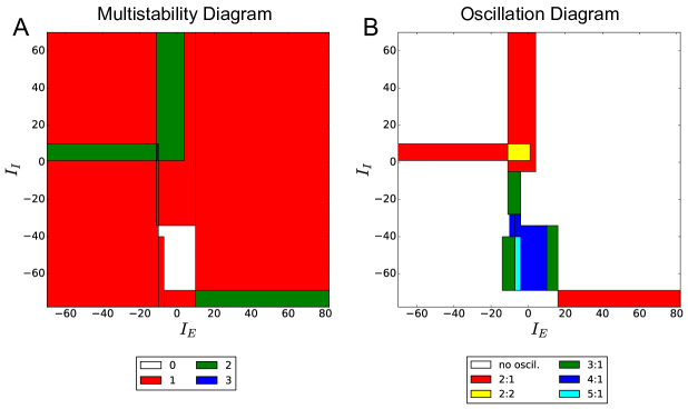
Figure 1: An example of bifurcation diagram. This figure shows the bifurcation diagram of the binary network, obtained for the parameters in Tab. (1). We supposed that the excitatory neurons with indexes $i=0$ and $i=1$ receive an arbitrary external stimulus $\mathfrak{I}_{0}=\mathfrak{I}_{1}=I_{E}$, which represents the first bifurcation parameter, while the excitatory neuron with index $i=2$ receives a fixed stimulus $\mathfrak{I}_{2}=10$. Moreover, we assumed that the inhibitory neuron with index $i=3$ receives an arbitrary stimulus $\mathfrak{I}_{3}=I_{I}$, which represents the second bifurcation parameter, while the inhibitory neuron with index $i=4$ receives a fixed stimulus $\mathfrak{I}_{4}=5$. Then, we plotted the multistability and oscillation diagrams in the $I_{E}-I_{I}$ plane, according to Eq. (2). A) Multistability diagram. Each color represents a different degree of multistability (white = astable, red = monostable, green = bistable, blue = tristable). B) Oscillation diagram. Each color represents a different set of oscillatory solutions of Eq. (1) (the notation $x:y$ reveals the formation of $y$ distinct oscillations with period $\mathcal{T}=x$). For example, for every combination of stimuli $\left(I_{E},I_{I}\right)$ that lies in the yellow area, Eq. (1) has $2$ oscillatory solutions with period $\mathcal{T}=2$, while for every combination in the green areas, the equation has an oscillatory solution with period $\mathcal{T}=3$. Note that, for other values of the network parameters, oscillations with distinct periods may coexist in the same area.

$J=\left[\begin{array}[]{ccccc}0&17&17&-43&-6\\ 25&0&15&-3&-32\\ 10&1&0&-10&-7\\ 50&29&6&0&-15\\ 7&28&5&-95&0\end{array}\right],\quad\theta_{0}=\cdots=\theta_{4}=1$

Table 1: Network parameters 1. This table reports the values of the network parameters that we used for plotting Figs. (1) - (4).

In this example, we consider a network with heterogeneous random synaptic weights, which is composed of $3$ excitatory neurons and $2$ inhibitory neurons. Moreover, in Fig. (2), we show two examples of state-to-state transitions, obtained by solving Eq. (1) in the zero-noise limit, for all the $2^{N}$ initial conditions of the network dynamics (i.e. from $\boldsymbol{A}\left(t=0\right)=\left[\begin{array}[t]{ccc}0,&\ldots,&0\end{array}\right]^{T}$ to $\boldsymbol{A}\left(t=0\right)=\left[\begin{array}[t]{ccc}1,&\ldots,&1\end{array}\right]^{T}$).

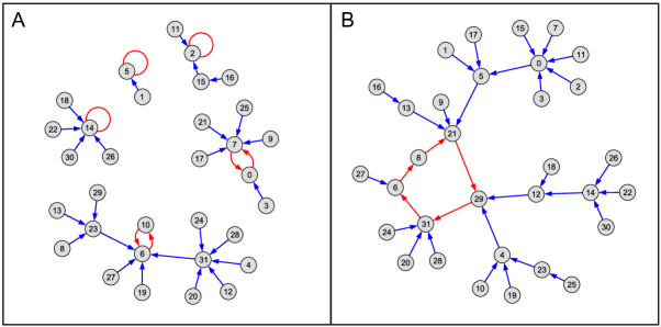
Figure 2: Examples of state-to-state transitions of a binary network. This figure shows the allowed transitions between states of neural activity, obtained for the network parameters in Tab. (1) and $\mathfrak{I}_{2}=10$, $\mathfrak{I}_{4}=5$. The nodes in the graphs represent the $2^{N}$ states of the neural activity vector $\boldsymbol{A}$ (e.g. the node $26$ corresponds to the state $\boldsymbol{A}=\left[\begin{array}[t]{ccccc}1,&1,&0,&1,&0\end{array}\right]^{T}$), while the arrows represent the allowed transitions between these states. A) State-to-state transitions, obtained for $I_{E}=-10.5$ and $I_{I}=6$. We highlighted in red $3$ stationary states (i.e. the nodes $2$, $5$ and $14$) and $2$ oscillations of period $\mathcal{T}=2$ (i.e. $0\rightarrow 7\rightarrow 0$ and $6\rightarrow 10\rightarrow 6$). Note that, as expected, the point in the stimulus plane with coordinates $\left(I_{E},I_{I}\right)=\left(-10.5,6\right)$ lies in the blue area of the multistability diagram (see Fig. (1), panel A), which corresponds to tristability, and in the yellow area of the oscillation diagram (see Fig. (1), panel B), which corresponds to the formation of $2$ oscillations with period $\mathcal{T}=2$. B) State-to-state transitions, obtained for $I_{E}=-5$ and $I_{I}=-55$. We highlighted in red an oscillations of period $\mathcal{T}=5$ (i.e. $6\rightarrow 8\rightarrow 21\rightarrow 29\rightarrow 31\rightarrow 6$). Note that the point in the stimulus plane with coordinates $\left(I_{E},I_{I}\right)=\left(-5,-55\right)$ lies in the white area of the multistability diagram, where Eq. (1) has no stationary solutions, and in the cyan area of the oscillation diagram, which corresponds to the formation of an oscillation with period $\mathcal{T}=5$.

4 Stochastic networks

4.1 Dualism between neural activity and membrane potentials

In this section we show the existence of a dualism between the neural activity states and the membrane potentials in a network composed of binary neurons. These variables are intrinsically related, but have distinct dynamical aspects.

As we explained in Sec. (2), the term $\sum_{j=0}^{N-1}J_{i,j}A_{j}\left(t\right)$ in Eq. (1) can be loosely interpreted as the weighted sum of postsynaptic potentials at neural dendrites. Therefore this term, plus the eventual external stimulus to the $i$th neuron, can be interpreted as the total membrane potential $V_{i}$ of that neuron, namely:

$$V_{i}\left(t+1\right)=\sum_{j=0}^{N-1}J_{i,j}A_{j}\left(t\right)+\mathfrak{I}_{i}+\sum_{j=0}^{N-1}\sigma_{i,j}^{\mathcal{N}}\mathcal{N}_{j}\left(t\right).$$ (3)

Since Eq. (1) does not depend on the variables $V_{i}\left(t\right)$, it can be solved without knowing the behavior of the membrane potentials. For this reason, the calculation of the probability distribution of $V_{i}\left(t\right)$ has always been neglected in the literature. Interestingly, we show that it is possible to exactly derive the set of equations satisfied by the membrane potentials, and that these equations provide a complementary description of the network dynamics with respect to Eq. (1). Under the change of variables Eq. (3), we observe that Eq. (1) can be equivalently transformed into the following set of equations:

$$V_{i}\left(t+1\right)=\sum_{j=0}^{N-1}J_{i,j}\mathscr{H}\left(V_{j}\left(t\right)-\theta_{j}\right)+\mathfrak{I}_{i}+\sum_{j=0}^{N-1}\sigma_{i,j}^{\mathcal{N}}\mathcal{N}_{j}\left(t\right),\quad i=0,...,N-1,$$ (4)

provided the matrix $J$ is invertible (note that this condition can be eventually relaxed, see the supplementary information of [29] for further details). Note also that Eqs. (1) and (3) imply $A_{i}\left(t\right)=\mathscr{H}\left(V_{i}\left(t\right)-\theta_{i}\right)\in\left\{0,1\right\}$, and that the binary output of a threshold unit can be loosely interpreted as the firing rate of that neuron: $A_{i}\left(t\right)=0$ if the $i$th neuron is not firing at time $t$, and $A_{i}\left(t\right)=1$ if it is firing at unit rate.

It is important to observe that the neural activities are discrete random variables, therefore they are described by probability mass functions (pmfs). We introduce the vector $\boldsymbol{A}=\left[\begin{array}[t]{ccc}A_{0},&\ldots,&A_{N-1}\end{array}\right]^{T}$ containing the activities of all $N$ neurons at time $t+1$, and $\boldsymbol{A}^{\prime}$ the vector of the activities of all neurons at time $t$. We also define:

$$\Psi\overset{\mathrm{def}}{=}\left[\begin{array}[]{ccc}\sigma_{0,0}^{\mathcal{N}}&\ldots&\sigma_{0,N-1}^{\mathcal{N}}\\ \vdots&\ddots&\vdots\\ \sigma_{N-1,0}^{\mathcal{N}}&\ldots&\sigma_{N-1,N-1}^{\mathcal{N}}\end{array}\right],\quad\boldsymbol{\theta}\overset{\mathrm{def}}{=}\left[\begin{array}[]{c}\theta_{0}\\ \vdots\\ \theta_{N-1}\end{array}\right],\quad\boldsymbol{\mathfrak{I}}\overset{\mathrm{def}}{=}\left[\begin{array}[]{c}\mathfrak{I}_{0}\\ \vdots\\ \mathfrak{I}_{N-1}\end{array}\right],\quad\boldsymbol{\mathscr{H}}\left(\boldsymbol{x}^{\prime}-\boldsymbol{\theta}\right)\overset{\mathrm{def}}{=}\left[\begin{array}[]{c}\mathscr{H}\left(x_{0}^{\prime}-\theta_{0}\right)\\ \vdots\\ \mathscr{H}\left(x_{N-1}^{\prime}-\theta_{N-1}\right)\end{array}\right],$$

where the matrix $\Psi$ is invertible by hypothesis. Moreover, we introduce the matrix $\mathcal{C}=\left[\mathcal{C}_{i,j}\right]_{i,j=0,\cdots,2^{N}-2}$, such that:

$$\mathcal{C}_{i,j}=\delta_{i,j}+G_{i,2^{N}-1}-G_{i,j},$$ (5)

where $\delta_{i,j}$ is the Kronecker delta, and:

$$G_{i,j}\overset{\mathrm{def}}{=}\frac{1}{\left|\det\left(\Psi\right)\right|}\int_{\mathscr{V}_{i}^{\left(N\right)}}p_{\boldsymbol{\mathcal{N}}}\left(\Psi^{-1}\left[\boldsymbol{x}-J\boldsymbol{\mathscr{B}}_{j}^{\left(N\right)}-\boldsymbol{\mathfrak{I}}\right]\right)d\boldsymbol{x},\quad i,j=0,\cdots,2^{N}-1.$$ (6)

In Eq. (6), $\boldsymbol{\mathscr{B}}_{i}^{\left(N\right)}$ is the $N\times 1$ vector whose entries are the digits of the binary representation of the index $i$ (e.g. $\boldsymbol{\mathscr{B}}_{39}^{\left(6\right)}=\left[\begin{array}[]{cccccc}1,&0,&0,&1,&1,&1\end{array}\right]^{T}$). Moreover, the set $\mathscr{V}_{i}^{\left(N\right)}$ is defined as follows:

$$\mathscr{V}_{i}^{\left(N\right)}\overset{\mathrm{def}}{=}\left\{\boldsymbol{x}\in\mathbb{R}^{N}:\;i=\mathscr{D}\left(\boldsymbol{\mathscr{H}}\left(\boldsymbol{x}-\boldsymbol{\theta}\right)\right)\right\},$$

where $\mathscr{D}\left(\boldsymbol{\nu}\right)$ is the decimal representation of the binary vector $\boldsymbol{\nu}$. For example, for $N=2$, we get:

$$\mathscr{V}_{0}^{\left(2\right)}= \left\{\left(x_{0},x_{1}\right)\in\mathbb{R}^{2}:x_{0}<\theta_{0},x_{1}<\theta_{1}\right\}$$

$$\mathscr{V}_{1}^{\left(2\right)}= \left\{\left(x_{0},x_{1}\right)\in\mathbb{R}^{2}:x_{0}<\theta_{0},x_{1}\geq\theta_{1}\right\}$$

$$\mathscr{V}_{2}^{\left(2\right)}= \left\{\left(x_{0},x_{1}\right)\in\mathbb{R}^{2}:x_{0}\geq\theta_{0},x_{1}<\theta_{1}\right\}$$

$$\mathscr{V}_{3}^{\left(2\right)}= \left\{\left(x_{0},x_{1}\right)\in\mathbb{R}^{2}:x_{0}\geq\theta_{0},x_{1}\geq\theta_{1}\right\}.$$

(note for example that, for any $\left(x_{0},x_{1}\right)\in\mathscr{V}_{3}^{\left(2\right)}$, we get $\left[\begin{array}[]{c}\mathscr{H}\left(x_{0}-\theta_{0}\right)\\ \mathscr{H}\left(x_{1}-\theta_{1}\right)\end{array}\right]=\left[\begin{array}[]{c}1\\ 1\end{array}\right]$, whose decimal representation is $3$). Finally, we define:

$$\widetilde{\boldsymbol{H}}=\left[\begin{array}[]{ccc}H_{0},&\ldots,&H_{2^{N}-2}\end{array}\right]^{T}\overset{\mathrm{def}}{=}\mathcal{C}^{-1}\widetilde{\boldsymbol{G}},\quad\widetilde{\boldsymbol{G}}\overset{\mathrm{def}}{=}\left[G_{i,2^{N}-1}\right]_{i=0,\ldots,2^{N}-2},\quad H_{2^{N}-1}\overset{\mathrm{def}}{=}1-\sum_{j=0}^{2^{N}-2}H_{j}.$$

Then, in [29] we proved that the conditional probability distribution of $\boldsymbol{A}$ given $\boldsymbol{A}^{\prime}$, and the stationary joint distribution of $\boldsymbol{A}$ in the limit $t\rightarrow+\infty$, are:

$$P\left(\boldsymbol{A},t+1|\boldsymbol{A}^{\prime},t\right)= \frac{1}{\left|\det\left(\Psi\right)\right|}\int_{\mathscr{V}_{\mathscr{D}\left(\boldsymbol{A}\right)}^{\left(N\right)}}p_{\boldsymbol{\mathcal{N}}}\left(\Psi^{-1}\left[\boldsymbol{x}-J\boldsymbol{A}^{\prime}-\boldsymbol{\mathfrak{I}}\right]\right)d\boldsymbol{x}$$ (7)

$$\underset{t\rightarrow+\infty}{\lim}P\left(\boldsymbol{A},t\right)= \frac{1}{\left|\det\left(\Psi\right)\right|}\sum_{j=0}^{2^{N}-1}H_{j}\int_{\mathscr{V}_{\mathscr{D}\left(\boldsymbol{A}\right)}^{\left(N\right)}}p_{\boldsymbol{\mathcal{N}}}\left(\Psi^{-1}\left[\boldsymbol{x}-J\boldsymbol{\mathscr{B}}_{j}^{\left(N\right)}-\boldsymbol{\mathfrak{I}}\right]\right)d\boldsymbol{x}.$$ (8)

On the other hand, the membrane potentials $V_{i}\left(t\right)$ are continuous variables, therefore they are described by probability density functions (pdfs). By introducing the vector $\boldsymbol{V}\overset{\mathrm{def}}{=}\left[\begin{array}[t]{ccc}V_{0},&\ldots,&V_{N-1}\end{array}\right]^{T}$, which contains the membrane potentials of all $N$ neurons at time $t+1$, and the vector $\boldsymbol{V}^{\prime}$ of the membrane potentials of all neurons at time $t$, the conditional probability distribution of $\boldsymbol{V}$ given $\boldsymbol{V}^{\prime}$, and the stationary joint distribution of $\boldsymbol{V}$ in the limit $t\rightarrow+\infty$, are [29]:

$$p\left(\boldsymbol{V},t+1|\boldsymbol{V}^{\prime},t\right)= \frac{1}{\left|\det\left(\Psi\right)\right|}p_{\boldsymbol{\mathcal{N}}}\left(\Psi^{-1}\left[\boldsymbol{V}-J\boldsymbol{\mathscr{H}}\left(\boldsymbol{V}^{\prime}-\boldsymbol{\theta}\right)-\boldsymbol{\mathfrak{I}}\right]\right)$$ (9)

$$\underset{t\rightarrow+\infty}{\lim}p\left(\boldsymbol{V},t\right)= \frac{1}{\left|\det\left(\Psi\right)\right|}\sum_{j=0}^{2^{N}-1}H_{j}p_{\boldsymbol{\mathcal{N}}}\left(\Psi^{-1}\left[\boldsymbol{V}-J\boldsymbol{\mathscr{B}}_{j}^{\left(N\right)}-\boldsymbol{\mathfrak{I}}\right]\right).$$ (10)

By comparing Eqs. (7) and (8) with, respectively, Eqs. (9) and (10), we observe that there exists a close relationship between the neural activities $\boldsymbol{A}$ and the membrane potentials $\boldsymbol{V}$, which we further investigate in SubSec. (4.2). It is also important to note that, generally, the integrals in Eqs. (5)-(8) can be calculated only numerically or through analytical approximations. However, in the specific case when the matrix $\Psi$ is diagonal, and the stochastic variables $\mathcal{N}_{i}\left(t\right)$ are independent, exact analytical solutions can be found in terms of the cumulative distribution functions of the noise sources (see [29]).

In Fig. (3) we show an example of the joint probability distributions $P\left(\boldsymbol{A},t\right)$ and $p\left(\boldsymbol{V},t\right)$ in the large-time limit, obtained for the network parameters that we reported in Tab. (1).

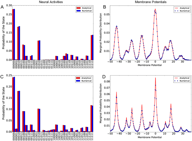
Figure 3: Probability distributions in stochastic networks. This figure shows the probability mass function $P\left(\boldsymbol{A},t\right)$ and the marginal probability density function $p\left(V_{i},t\right)$ of the $0$th neuron, obtained for the network parameters in Tab. (1), $\boldsymbol{\mathfrak{I}}=\left[\begin{array}[]{ccccc}0,&-3,&2,&-4,&0\end{array}\right]^{T}$, $\Psi=\mathrm{diag}\left(\begin{array}[]{ccccc}2,&3,&2,&3,&3\end{array}\right)$, and $t=100$. A) - B) Probability distributions obtained for correlated normally-distributed noise sources, with uniform cross-correlation (namely $\mathrm{Corr}\left(\mathcal{N}_{i}\left(t\right),\mathcal{N}_{j}\left(t\right)\right)=0.8$ and $\mathrm{Corr}\left(\mathcal{N}_{i}\left(t\right),\mathcal{N}_{j}\left(s\right)\right)=0$, for $t\neq s$ and $\forall i,\,j$). C) - D) Probability distributions obtained for independent noise sources with Laplace distributions, namely $p_{\boldsymbol{\mathcal{N}}}\left(\boldsymbol{x}\right)=\prod_{i=0}^{N-1}p_{\mathcal{N}_{i}}\left(x_{i}\right)$, where $p_{\mathcal{N}_{i}}\left(x_{i}\right)=\frac{\sqrt{2}}{2}\exp\left(-\sqrt{2}\left|x_{i}\right|\right)$. The red bars in panels A and C are calculated analytically from Eq. (8), while the red curves in panels B and D are calculated according to Eq. (10). The blue bars in panels A, C, and the blue dots in panels B, D are calculated numerically through a Monte Carlo method, namely by solving Eq. (1) $10,000$ times, and then by calculating the probability distributions across the repetitions.

In this figure we considered two distinct distributions of the noise sources (namely correlated normally-distributed variables $\mathcal{N}_{i}\left(t\right)$, as well as independent sources with Laplace distributions), and we showed how they differently shape the probability distributions of the neural activity and of the membrane potentials.

4.2 Cross-neuron correlations

The joint probability distributions $P\left(\boldsymbol{A},t\right)$ and $p\left(\boldsymbol{V},t\right)$, that we reported in the previous section, provide a complete probabilistic description of the network in the limit $t\rightarrow+\infty$. In particular, these distributions can be used for calculating cross-neuron correlations, which represents a powerful tool for quantifying the exchange of information between neurons. In [29], we derived exact analytical expressions of the Pearson correlation coefficient for $t\rightarrow+\infty$, in the case when the matrix $\Psi$ is diagonal (i.e. $\Psi=\mathrm{diag}\left(\sigma_{0}^{\mathcal{N}},\ldots,\sigma_{N-1}^{\mathcal{N}}\right)$, where $\sigma_{i}^{\mathcal{N}}\overset{\mathrm{def}}{=}\sigma_{i,i}^{\mathcal{N}}\;\forall i$), while the noise sources are independent and normally distributed. By applying Eq. (8), we found that the pairwise correlation between the neural activities of two neurons with indexes $i$ and $j$ is:

$$\mathrm{Corr}\left(A_{i},A_{j}\right)= \frac{\mathrm{Cov}\left(A_{i},A_{j}\right)}{\sqrt{\mathrm{Var}\left(A_{i}\right)\mathrm{Var}\left(A_{j}\right)}}$$

$$\mathrm{Cov}\left(A_{i},A_{j}\right)= \frac{1}{4}\sum_{n=0}^{2^{N}-1}H_{n}\left(1-2\overline{A}_{i}-E_{n,i}\right)\left(1-2\overline{A}_{j}-E_{n,j}\right)$$

$$\mathrm{Var}\left(A_{i}\right)= \overline{A}_{i}-\left(\overline{A}_{i}\right)^{2}$$ (11)

$$\overline{A}_{i}= \frac{1}{2}\left(1-\sum_{n=0}^{2^{N}-1}H_{n}E_{n,i}\right)$$

$$E_{n,i}= \mathrm{erf}\left(\frac{\theta_{i}-\sum_{m=0}^{N-1}J_{i,m}\mathscr{B}_{n,m}^{\left(N\right)}-\mathfrak{I}_{i}}{\sqrt{2}\sigma_{i}^{\mathcal{N}}}\right).$$

In a similar way, from Eq. (10) we derived the following formula for the pairwise correlation between the membrane potentials:

$$\mathrm{Corr}\left(V_{i},V_{j}\right)= \frac{\mathrm{Cov}\left(V_{i},V_{j}\right)}{\sqrt{\mathrm{Var}\left(V_{i}\right)\mathrm{Var}\left(V_{j}\right)}}$$

$$\mathrm{Cov}\left(V_{i},V_{j}\right)= \sum_{n=0}^{2^{N}-1}H_{n}\mathcal{R}_{n,i}^{\left(N\right)}\mathcal{R}_{n,j}^{\left(N\right)}$$

$$\mathrm{Var}\left(V_{i}\right)= \left(\sigma_{i}^{\mathcal{N}}\right)^{2}+\sum_{n=0}^{2^{N}-1}H_{n}\left(\mathcal{R}_{n,i}^{\left(N\right)}\right)^{2}$$

$$\mathcal{R}_{n,i}^{\left(N\right)}\overset{\mathrm{def}}{=} \sum_{m=0}^{N-1}\left[\left(\mathscr{B}_{n,m}^{\left(N\right)}-\sum_{k=0}^{2^{N}-1}H_{k}\mathscr{B}_{k,m}^{\left(N\right)}\right)J_{i,m}\right].$$

In Fig. (4) we plotted some examples of cross-correlations, obtained for the the network parameters that we reported in Tab. (1).

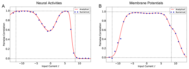
Figure 4: Cross-neuron correlations. This figure shows the dependence of the cross-neuron correlation of the binary network on the external stimulus, in the specific case of independent normally-distributed noise sources. Correlation is calculated between the neurons with indexes $i=0$ and $i=4$, for the values of the parameters reported in Tab. (1), $\boldsymbol{\mathfrak{I}}=I\left[\begin{array}[]{ccccc}1,&1,&1,&1,&1\end{array}\right]^{T}$, $I\in\left[-14,14\right]$, $\Psi=\mathrm{diag}\left(\begin{array}[]{ccccc}2,&3,&2,&3,&3\end{array}\right)$, and $t=100$. A) Correlation between neural activities. The red curve is calculated analytically from Eq. (11). B) Correlation between membrane potentials. The red curve is calculated according to Eq. (LABEL:eq:correlation-between-the-membrane-potentials). In both panels, the blue dots are calculated numerically through a Monte Carlo method over $10,000$ repetitions. Moreover, the vertical dashed lines correspond to the stimuli $I=-12$ and $I=8.5$. We chose these values of the stimuli to show that low (respectively high) correlations between neural activities do not necessarily correspond to low (respectively high) correlations between the membrane potentials ($\mathrm{Corr}\left(A_{0},A_{4}\right)\approx 0.99$ and $\mathrm{Corr}\left(V_{0},V_{4}\right)\approx 0.02$ for $I=-12$, while $\mathrm{Corr}\left(A_{0},A_{4}\right)\approx 0.06$ and $\mathrm{Corr}\left(V_{0},V_{4}\right)\approx 0.65$ for $I=8.5$).

This figure shows that variations of the external stimuli $\boldsymbol{\mathfrak{I}}$ switches the binary network between synchronous (i.e. highly correlated) and asynchronous (i.e. uncorrelated) states. Moreover, we observe that low (respectively high) correlations between neural activities do not necessarily correspond to low (respectively high) correlations between the membrane potentials. In other words, the linear relationship between the neural activity and the membrane potentials, as given by Eq. (3), is not reflected by the correlation structure of these variables. This result proves that, despite the similarity of the corresponding equations (which we already observed in SubSec. (4.1), by comparing Eqs. (7) and (8) with, respectively, Eq. (9) and (10)) and their linear relationship, neural activity and the membrane potentials represent two opposed aspects of binary networks.

The interested reader is referred to [29] for a detailed description of the conditions under which synchronous and asynchronous states occur in the network, and for the extension of Eqs. (11) and (LABEL:eq:correlation-between-the-membrane-potentials) to encompass higher-order (i.e. groupwise) correlations among an arbitrary number of neurons.

4.3 Pattern storage and retrieval in presence of noise

In this section we consider the problem of storing $\mathcal{D}$ sequences of neural activity vectors $\boldsymbol{A}^{\left(i,0\right)}\rightarrow\boldsymbol{A}^{\left(i,1\right)}\rightarrow\cdots\rightarrow\boldsymbol{A}^{\left(i,\mathcal{T}_{i}\right)}$, for $i=0,\ldots,\mathcal{D}-1$. In the context of content-addressable memories, one aims to determine a synaptic connectivity matrix $J$ that stores these sequences in the binary network, so that each sequence can be retrieved by initializing the network state to $\boldsymbol{A}\left(t=0\right)=\boldsymbol{A}^{\left(i,0\right)}$, even in the presence of noise. Any method for calculating such a connectivity matrix is typically called learning rule.

Each transition $\boldsymbol{A}^{\left(i,n_{i}\right)}\rightarrow\boldsymbol{A}^{\left(i,n_{i}+1\right)}$ in the sequences is noise-resistant whenever
$P\left(\boldsymbol{A}^{\left(i,n_{i}+1\right)},t_{n_{i}}+1|\boldsymbol{A}^{\left(i,n_{i}\right)},t_{n_{i}}\right)\approx 1$, since under this condition the probability that the state $\boldsymbol{A}^{\left(i,n_{i}\right)}$ switches to a state other than $\boldsymbol{A}^{\left(i,n_{i}+1\right)}$ at the time instant $t_{n_{i}}+1$ is negligible. Therefore, according to Eq. (7), the sequences of neural activity can be stored in the network by solving the following set of equations:

$$\int_{\mathscr{V}_{\mathscr{D}\left(\boldsymbol{A}\right)}^{\left(N\right)}}p_{\mathcal{N}}\left(\Psi^{-1}\left[\boldsymbol{x}-J\boldsymbol{A}^{\prime}-\boldsymbol{\mathfrak{I}}\right]\right)d\boldsymbol{x}\approx\left|\det\left(\Psi\right)\right|,\quad\left(\boldsymbol{A}^{\prime},\boldsymbol{A}\right)=\left(\boldsymbol{A}^{\left(i,n_{i}\right)},\boldsymbol{A}^{\left(i,n_{i}+1\right)}\right),\quad n_{i}=0,\ldots,\mathcal{T}_{i}-1,\quad i=0,\ldots,\mathcal{D}-1$$

with respect to the connectivity matrix $J$. Generally, these equations can be solved only numerically or through analytical approximations. However, in the specific case when the matrix $\Psi$ is diagonal and the stochastic variables $\mathcal{N}_{i}\left(t\right)$ are independent, exact analytical solutions can be found.

In [29], we considered the case of of independent normally-distributed noise sources, and we found that, if the network is fully-connected without self connections (so that $J_{i,i}=0$), the matrix $J$ that stores the $\mathcal{D}$ neural sequences satisfies the following sets of linear algebraic equations:

$$\Omega^{\left(j\right)}\boldsymbol{J}^{\left(j\right)}=\boldsymbol{u}^{\left(j\right)},\quad j=0,\ldots,N-1.$$ (13)

In Eq. (13), $\boldsymbol{J}^{\left(j\right)}$ is the $\left(N-1\right)\times 1$ vector with entries $J_{j,k}$ for $k\neq j$. Moreover, if we define $\mathscr{T}\overset{\mathrm{def}}{=}\sum_{i=0}^{\mathcal{D}-1}\mathcal{T}_{i}$, $\mathfrak{T}_{i}\overset{\mathrm{def}}{=}\sum_{k=1}^{i}\mathcal{T}_{k-1}$ (for $i>0$) and $\mathfrak{T}_{0}\overset{\mathrm{def}}{=}0$, then $\boldsymbol{u}^{\left(j\right)}$ is a $\mathscr{T}\times 1$ vector with entries:

$$\left[\boldsymbol{u}^{\left(j\right)}\right]_{\mathfrak{T}_{i}+n_{i}}=\theta_{j}-\left(-1\right)^{A_{j}^{\left(i,n_{i}+1\right)}}K_{j}^{\left(i,n_{i}\right)}\sqrt{2}\sigma_{j}^{\mathcal{N}}-\mathfrak{I}_{j},\quad n_{i}=0,\ldots,\mathcal{T}_{i}-1,\quad i=0,\ldots,\mathcal{D}-1,$$

where $K_{j}^{\left(i,n_{i}\right)}$ is any sufficiently large and positive constant. Moreover, in Eq. (13), $\Omega^{\left(j\right)}$ is the $\mathscr{T}\times\left(N-1\right)$ matrix obtained by removing the $j$th column of the following matrix:

$$\Omega=\left[\begin{array}[]{ccc}A_{0}^{\left(0,0\right)}&\ldots&A_{N-1}^{\left(0,0\right)}\\ \vdots&\ddots&\vdots\\ A_{0}^{\left(0,\mathcal{T}_{0}-1\right)}&\ldots&A_{N-1}^{\left(0,\mathcal{T}_{0}-1\right)}\\ \vdots&\ddots&\vdots\\ A_{0}^{\left(\mathcal{D}-1,0\right)}&\ldots&A_{N-1}^{\left(\mathcal{D}-1,0\right)}\\ \vdots&\ddots&\vdots\\ A_{0}^{\left(\mathcal{D}-1,\mathcal{T}_{\mathcal{D}-1}-1\right)}&\ldots&A_{N-1}^{\left(\mathcal{D}-1,\mathcal{T}_{\mathcal{D}-1}-1\right)}\end{array}\right].$$

In particular, we observe that whenever $\boldsymbol{A}^{\left(i,0\right)}=\boldsymbol{A}^{\left(i,\mathcal{T}_{i}\right)}$, the $i$th neural sequence is an oscillatory solution of Eq. (1) with period $\mathcal{T}_{i}$, so that if the matrix $J$ is calculated by solving Eq. (13) and the network is initialized to any state of the oscillation, the network will cycle repeatedly through the same set of states. Moreover, in the special case $\mathcal{T}=1$, the neural sequence represents a stationary solution of Eq. (1) .

In Fig. (5), we show some examples of storage of stationary patterns and oscillatory sequences with $\mathscr{T}=3$. This figure is obtained for the the network parameters reported in Tab. (2), and proves that the learning rule Eq. (13) can be used to store safely sequences of neural activity also in very noisy networks.

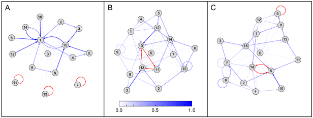
Figure 5: Storage of activity patterns and neural sequences. This figure shows examples of activity patterns and neural sequences (highlighted in red), stored in a stochastic binary network, for $N=4$, $\boldsymbol{\mathfrak{I}}=\left[\begin{array}[]{cccc}0,&0,&0,&0\end{array}\right]^{T}$, and $\Psi=\mathrm{diag}\left(\begin{array}[]{cccc}50,&50,&50,&50\end{array}\right)$. The color gradation of the blue arrows is proportional to the magnitude of $P\left(\boldsymbol{A}^{\left(i,n_{i}+1\right)},t_{n_{i}}+1|\boldsymbol{A}^{\left(i,n_{i}\right)},t_{n_{i}}\right)$ (see Eq. (7)), so that the arrows are white for every pair of states $\left(\boldsymbol{A}^{\left(i,n_{i}\right)},\boldsymbol{A}^{\left(i,n_{i}+1\right)}\right)$ such that $P\left(\boldsymbol{A}^{\left(i,n_{i}+1\right)},t_{n_{i}}+1|\boldsymbol{A}^{\left(i,n_{i}\right)},t_{n_{i}}\right)\approx 0$, while they are blue if the conditional probability is close to $1$. The noise sources are supposed to be independent and normally distributed, so that the synaptic connectivity matrix $J$ that stores the patterns can be calculated according to Eq. (13). In these examples, we set $K_{j}^{\left(i,n_{i}\right)}=10\;\forall i,\>,j,\>,n_{i}$, while the matrices $\Omega$ and the corresponding solutions $J$ are reported in Tab. (2). A) Storage of $3$ stationary states, highlighted in red. B) Storage of an oscillation with period $\mathcal{T}=3$. C) Storage of a stationary state and an oscillation with period $\mathcal{T}=2$. Note that the stationary states and the oscillations are noise-resistant, despite the presence of strong noise sources ($\sigma_{i}^{\mathcal{N}}=50\;\forall i$).

Panel A	Panel B	Panel C
$\Omega=\left[\begin{array}[]{cccc}1&1&0&1\\ 0&1&1&1\\ 1&0&1&1\end{array}\right]$	$\Omega=\left[\begin{array}[]{cccc}1&0&1&1\\ 1&1&0&1\\ 1&0&1&0\end{array}\right]$	$\Omega=\left[\begin{array}[]{cccc}0&1&0&1\\ 1&1&1&0\\ 1&0&0&1\end{array}\right]$
$J\approx\left[\begin{array}[]{cccc}0&-1414&-1414&2122\\ -1414&0&-1414&2122\\ -1414&-1414&0&2122\\ 354&354&354&0\end{array}\right]$	$J\approx\left[\begin{array}[]{cccc}0&708&708&0\\ -2120&0&1414&1414\\ 708&1414&0&-1414\\ 1&-707&707&0\end{array}\right]$	$J\approx\left[\begin{array}[]{cccc}0&0&-706&708\\ -1414&0&2122&708\\ -1060&354&0&354\\ 708&-706&706&0\end{array}\right]$

Table 2: Network parameters 2. This table reports the matrices $\Omega$ and the corresponding matrices $J$, that we used for plotting Fig. (5).

5 Networks with quenched disorder

The results reported in Secs.  (3) and (4) are valid for binary neural networks with arbitrary topology of the synaptic connections (which does not evolve over time). For this reason, they can be applied to networks with regular connectivity matrices $J$, as well as to random networks with frozen synaptic weights (see e.g. the network parameters reported in Tab. (1)). In other words, the connectivity matrix of random networks can be interpreted as a single realization of the synaptic wiring among neurons, generated according to some known probability distribution $p_{J}$. These models are said to present quenched disorder [70, 43, 39].

Each realization of the connectivity matrix, generated according to the distribution $p_{J}$, usually produces a distinct matrix $J$, which in turn gives rise to distinct dynamical properties of the neural activity. In particular, each realization typically produces distinct bifurcation diagrams. For this reason, in order to obtain statistically representative results, one needs to average the coordinates of the bifurcation points over the variability of the matrix $J$. More generally, one would be interested in determining the probability distribution of the bifurcation points over the matrix $J$.

In [30] we derived semi-analytical expressions of these probability distributions. For simplicity, we focused on the bifurcation points of the stationary states in the zero-noise limit ($\sigma_{i,j}^{\mathcal{N}}\rightarrow 0\;\forall i,j$ ). We supposed that the entries $J_{i,j}$ of the connectivity matrix can be decomposed as the product of a synaptic weight, $W_{i,j}$ (which represents the random strength of interaction of the $j$th neuron on the $i$th neuron), with another random variable, $T_{i,j}$ (which represents either the presence, for $T_{i,j}=1$, or the absence, for $T_{i,j}=0$, of a synaptic connections from the $j$th to the $i$th neuron). The random variable $W_{i,j}$ is supposed to be continuous, and distributed according to some distribution $p_{W_{i,j}}$. On the other hand, the variable $T_{i,j}$ is discrete, and such that $T_{i,j}=1$ with probability $\mathcal{P}_{i,j}\in\left[0,1\right]$, while $T_{i,j}=0$ with probability $1-\mathcal{P}_{i,j}$. We also supposed that the variables $\left\{W_{i,j},T_{i,j}\right\}_{i,j=0,\cdots,N-1}$ are statistically independent. Because of these assumptions, the random variable $\mathcal{I}_{i}$ (as given by Eq. (2); note that the superscript $\left(j\right)$ can be omitted in the case of stationary states studied in this section) is distributed as follows:

$$p_{\mathcal{I}_{i}}\left(x\right)= a_{i}\left(\theta_{i}-x\right)+b_{i}\delta\left(\theta_{i}-x\right)$$

$$a_{i}\left(x\right)= \sum_{\mathscr{S}\in\mathbb{P}\left(R\right)\backslash\emptyset}\left[\prod_{j\in\mathscr{S}}\mathcal{P}_{i,j}\right]\left[\prod_{j\in R\backslash\mathscr{S}}\left(1-\mathcal{P}_{i,j}\right)\right]\left[\left(\operatorname*{\raisebox{-3.09999pt}{\scalebox{2.5}{$\ast$}}}_{j\in\mathscr{S}}p_{W_{i,j}}\right)\left(x\right)\right]$$

$$b_{i}= \prod_{j\in R}\left(1-\mathcal{P}_{i,j}\right),$$

where $\mathbb{P}\left(R\right)$ represents the power set of $R\overset{\mathrm{def}}{=}\left\{i\in\left\{0,\cdots,N-1\right\}:\;A_{i}=1\right\}$. Moreover, we call $F_{\mathcal{I}_{i}}$ the cumulative distribution function of $\mathcal{I}_{i}$. Then, the coordinates of the bifurcation points, $\Lambda_{\alpha}$ and $\Xi_{\alpha}$, are distributed as follows:

$$p_{X}\left(x\right)=p_{X^{c}}\left(x\right)+\sum_{q\in D}\left[F_{X}\left(x_{q}\right)-\underset{x\rightarrow x_{q}^{-}}{\lim}F_{X}\left(x\right)\right]\delta\left(x-x_{q}\right),$$ (14)

for $X\in\left\{\Lambda_{\alpha},\Xi_{\alpha}\right\}$. In Eq. (14), $\delta\left(\cdot\right)$ is the Dirac delta function, $p_{X^{c}}$ is the component of $p_{X}$ that describes the statistical behavior of the continuous values of $X$, and $F_{X}$ is the cumulative distribution function of $X$. Since, according to Eq. (2), $\Lambda_{\alpha}$ and $\Xi_{\alpha}$ are, respectively, the maximum and minimum of the independent variables $\mathcal{I}_{i}$, they must be distributed according to order statistics [75, 10, 9, 36]. By calling $\mathrm{per}\left(\cdot\right)$ the matrix permanent, in [30] we proved that $X^{c}$ is distributed as follows:

$$p_{\Lambda_{\alpha}^{c}}\left(x\right)= \frac{1}{\left(\gamma_{\alpha,1}-1\right)!}\mathrm{per}\left(\left[\begin{array}[]{cc}\boldsymbol{a}_{\alpha,1}\left(\boldsymbol{\theta}-\boldsymbol{x}\right),&\boldsymbol{F}_{\alpha,1}^{\left(\gamma_{\alpha,1}-1\right)}\left(x\right)\end{array}\right]\right)$$ (16)

$$p_{\Xi_{\alpha}^{c}}\left(x\right)= \frac{1}{\left(\gamma_{\alpha,0}-1\right)!}\mathrm{per}\left(\left[\begin{array}[]{cc}\boldsymbol{a}_{\alpha,0}\left(\boldsymbol{\theta}-\boldsymbol{x}\right),&\mathbb{I}_{\gamma_{\alpha,0},\gamma_{\alpha,0}-1}-\boldsymbol{F}_{\alpha,0}^{\left(\gamma_{\alpha,0}-1\right)}\left(x\right)\end{array}\right]\right),$$ (19)

where $\gamma_{\alpha,u}\overset{\mathrm{def}}{=}\left|\Gamma_{I_{\alpha},u}\right|$, while $\left[\begin{array}[]{cc}\boldsymbol{a}_{\alpha,1}\left(\boldsymbol{\theta}-\boldsymbol{x}\right),&\boldsymbol{F}_{\alpha,1}^{\left(\gamma_{\alpha,1}-1\right)}\left(x\right)\end{array}\right]$ and
$\left[\begin{array}[]{cc}\boldsymbol{a}_{\alpha,0}\left(\boldsymbol{\theta}-\boldsymbol{x}\right),&\mathbb{I}_{\gamma_{\alpha,0},\gamma_{\alpha,0}-1}-\boldsymbol{F}_{\alpha,0}^{\left(\gamma_{\alpha,0}-1\right)}\left(x\right)\end{array}\right]$ are $\gamma_{\alpha,1}\times\gamma_{\alpha,1}$ and $\gamma_{\alpha,0}\times\gamma_{\alpha,0}$ matrices respectively,
$\boldsymbol{a}_{\alpha,u}\left(\boldsymbol{\theta}-\boldsymbol{x}\right)\overset{\mathrm{def}}{=}\left[a_{i}\left(\theta_{i}-x\right)\right]_{i\in\Gamma_{I_{\alpha},u}}$ and $\boldsymbol{F}_{\alpha,u}\left(x\right)\overset{\mathrm{def}}{=}\left[F_{\mathcal{I}_{i}}\left(x\right)\right]_{i\in\Gamma_{I_{\alpha},u}}$ are $\gamma_{\alpha,u}\times 1$ column vectors, $\boldsymbol{F}_{\alpha,u}^{\left(v\right)}\left(x\right)\overset{\mathrm{def}}{=}\underset{v-\mathrm{times}}{\left[\underbrace{\begin{array}[]{ccc}\boldsymbol{F}_{\alpha,u}\left(x\right),&\cdots,&\boldsymbol{F}_{\alpha,u}\left(x\right)\end{array}}\right]}$ is a $\gamma_{\alpha,u}\times v$ matrix, and $\mathbb{I}_{\gamma_{\alpha,0},\gamma_{\alpha,0}-1}$ is the $\gamma_{\alpha,0}\times\left(\gamma_{\alpha,0}-1\right)$ all-ones matrix. Moreover, in Eq. (14), $\left\{x_{q}\right\}_{q\in D}$ represents the set of the discrete values of $X$, at which the cumulative distribution function $F_{X}$, namely:

$$F_{\Lambda_{\alpha}}\left(x\right)= \frac{1}{\gamma_{\alpha,1}!}\mathrm{per}\left(\left[\boldsymbol{F}_{\alpha,1}^{\left(\gamma_{\alpha,1}\right)}\left(x\right)\right]\right)$$

$$F_{\Xi_{\alpha}}\left(x\right)= \sum_{n=1}^{\gamma_{\alpha,0}}\frac{1}{n!\left(\gamma_{\alpha,0}-n\right)!}\mathrm{per}\left(\left[\begin{array}[]{cc}\boldsymbol{F}_{\alpha,0}^{\left(n\right)}\left(x\right),&\mathbb{I}_{\gamma_{\alpha,0},\gamma_{\alpha,0}-n}-\boldsymbol{F}_{\alpha,0}^{\left(\gamma_{\alpha,0}-n\right)}\left(x\right)\end{array}\right]\right),$$ (22)

is (possibly) discontinuous. Note that $D=\Gamma_{I_{\alpha},1}$ and $D=\Gamma_{I_{\alpha},0}$, for $\Lambda_{\alpha}$ and $\Xi_{\alpha}$ respectively, while $x_{q}=\theta_{q}$.

The mean multistability diagram of the network is the plot of the bifurcation points $\Lambda_{\alpha}$ and $\Xi_{\alpha}$, averaged over the realizations of the synaptic connectivity matrix $J$. In other words, the mean bifurcation points $\left\langle\Lambda_{\alpha}\right\rangle$ and $\left\langle\Xi_{\alpha}\right\rangle$ (where the brackets $\left\langle\cdot\right\rangle$ represent the mean over the realizations) correspond to the values of the stimulus $I_{\alpha}$ at which a given neural activity state $\boldsymbol{A}$ loses its stability on average, turning into another stationary state or an oscillation. In [30] we proved that:

$$\left\langle X\right\rangle=\int_{-\infty}^{+\infty}xp_{X^{c}}\left(x\right)dx+\sum_{q\in D}x_{q}\left[F_{X}\left(x_{q}\right)-\underset{x\rightarrow x_{q}^{-}}{\lim}F_{X}\left(x\right)\right]=\int_{-\infty}^{+\infty}\left[\mathscr{H}\left(x\right)-F_{X}\left(x\right)\right]dx,$$ (23)

where the functions $p_{X^{c}}\left(x\right)$ and $F_{X}\left(x\right)$ are given, respectively, by Eqs. (LABEL:eq:continuous-components) and (LABEL:eq:cumulative-distribution-functions).

The probability that a given activity state $\boldsymbol{A}$ is stationary for a fixed combination of stimuli $\widehat{\boldsymbol{I}}=\left[\begin{array}[]{ccc}\widehat{I}_{0},&\cdots,&\widehat{I}_{\mathfrak{P}-1}\end{array}\right]^{T}$, corresponds to the probability that $\widehat{\boldsymbol{I}}\in\mathfrak{V}$, where the coordinates of the hyperrectangle $\mathfrak{V}$ are calculated from Eq. (2) for the given state $\boldsymbol{A}$. In [30] we proved that this probability can be calculated from the cumulative distribution of the bifurcation points as follows:

$$P\left(\widehat{\boldsymbol{I}}\in\mathfrak{V}\right)=\prod_{\alpha=0}^{\mathfrak{P}-1}P\left(\widehat{I}_{\alpha}\in\mathcal{V}_{\alpha}\right)$$ (24)

$$P\left(\widehat{I}_{\alpha}\in\mathcal{V}_{\alpha}\right)=\begin{cases}1-F_{\Xi_{\alpha}}\left(\widehat{I}_{\alpha}\right),&\mathrm{if}\;\;\Gamma_{I_{\alpha},1}=\emptyset\\ \\ F_{\Lambda_{\alpha}}\left(\widehat{I}_{\alpha}\right),&\mathrm{if}\;\;\Gamma_{I_{\alpha},0}=\emptyset\\ \\ F_{\Lambda_{\alpha}}\left(\widehat{I}_{\alpha}\right)\left[1-F_{\Xi_{\alpha}}\left(\widehat{I}_{\alpha}\right)\right],&\mathrm{otherwise}.\end{cases}$$

Moreover, the probability to observe the state $\boldsymbol{A}$ in the whole multistability diagram of a single realization of the matrix $J$ (i.e. the probability that $\boldsymbol{A}$ is stationary, regardless of the specific combination of stimuli), corresponds to the probability that the hyperrectangle $\mathfrak{V}$ has positive hypervolume $\mathrm{vol}\left(\mathscr{V}\right)$. In [30] we proved that this probability has the following expression:

$$P\left(\mathrm{vol}\left(\mathfrak{V}\right)>0\right)=\prod_{\alpha=0}^{\mathfrak{P}-1}\left[\int_{-\infty}^{+\infty}p_{\Xi_{\alpha}^{c}}\left(x\right)F_{\Lambda_{\alpha}}\left(x\right)dx+\sum_{q\in\Gamma_{I_{\alpha},0}}\left[F_{\Xi_{\alpha}}\left(\theta_{q}\right)-\underset{x\rightarrow\theta_{q}^{-}}{\lim}F_{\Xi_{\alpha}}\left(x\right)\right]F_{\Lambda_{\alpha}}\left(\theta_{q}\right)\right].$$ (25)

Eqs. (14)-(25) provide a complete description of the statistical properties of the stationary states in networks with quenched disorder. It is also important to note that these equations are semi-analytical, since they are expressed in terms of 1D integrals containing the distribution $p_{W_{i,j}}$. These integrals may be calculated exactly for some $p_{W_{i,j}}$, for example in the case of normally-distributed weights. However, for simplicity, in this review and in [30], they are calculated through numerical integration schemes, because fully-analytical expressions may be very cumbersome.

In Figs. (6) and (7) we show an example of these results for a specific distribution of the connectivity matrix.

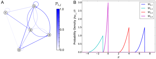
Figure 6: Probability distribution of the synaptic connections. This figure reports the probability distribution of the network topology and of the synaptic weights, given the values of the network parameters reported in Tab. (3). A) Probability distribution of the network topology, namely the graph of the matrix $\left[\mathcal{P}_{i,j}\right]_{i,j=0,\cdots,N-1}$. The $N=5$ nodes in the graph represent the neurons in the network, while the arrow from the $j$th to the $i$th neuron represents the probability to observe the $i\leftarrow j$ synaptic connection in a single realization of the matrix $J$ (note that the color gradation is proportional to $\mathcal{P}_{i,j}$). B) Examples of the powerlaw probability distributions of the synaptic weights $W_{i,j}$, see Eq. (26).

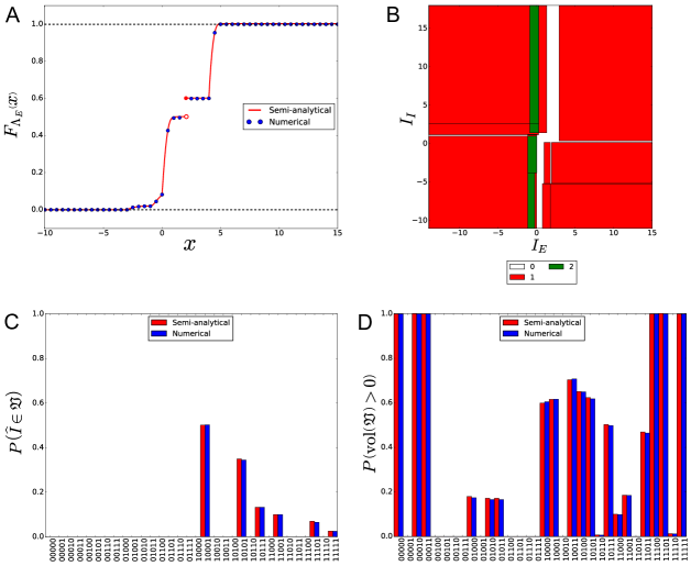
Figure 7: Stationary behavior of a binary network with quenched disorder. This figure reports the probabilistic properties of the stationary states of a binary network with quenched disorder. The matrix $J$ is generated randomly from the powerlaw distribution Eq. (26), and for the network parameters in Tab. (3) (see also Fig. (6)). A) Cumulative distribution function $F_{\Lambda_{E}}\left(x\right)$ of the activity state $\boldsymbol{A}=\left[\begin{array}[]{ccccc}1,&0,&1,&1,&0\end{array}\right]^{T}$. The red curve is derived semi-analytically from Eq. (LABEL:eq:cumulative-distribution-functions), while the blue dots are calculated numerically through a Monte Carlo method over $10,000$ repetitions of the synaptic connectivity matrix. B) Mean multistability diagram of the network, obtained semi-analytically from Eq. (23). C) -D) Occurrence probability of the stationary states, obtained for the fixed stimuli $\left[\begin{array}[]{c}I_{E}\\ I_{I}\end{array}\right]=\widehat{\boldsymbol{I}}=\left[\begin{array}[]{c}1\\ 0\end{array}\right]$ (panel C), and regardless of the stimuli (panel D). The red bars in panel C (respectively, panel D) are derived semi-analytically from Eq. (24) (respectively, Eq. (25)), while the blue bars are calculated numerically through a Monte Carlo method (see [30] for more details).

We consider a network composed of $3$ excitatory neurons (with indexes $i=0,1,2$), and $2$ inhibitory neurons ($i=3,4$). The excitatory and inhibitory neurons receive, respectively, external stimuli $I_{E}$ and $I_{I}$. We also assume that the synaptic weights $W_{i,j}$ are distributed according to the following powerlaw distribution:

$$p_{W_{i,j}}\left(x\right)=\begin{cases}\frac{3}{\mathfrak{W}}\left(\frac{x-\mathfrak{S}}{\mathfrak{W}}\right)^{2},&\mathrm{if}\;\;\mathfrak{S}\leq x\leq\mathfrak{S}+\mathfrak{W}\\ \\ 0,&\mathrm{otherwise},\end{cases}$$ (26)

where $\mathfrak{S}$ and $\mathfrak{W}$ represent, respectively, the horizontal shift and the width of the support of the distribution. To conclude, in Tab. (3) we reported the values of the parameters $\mathcal{P}$, $\boldsymbol{\theta}$, $\mathfrak{S}$ and $\mathfrak{W}$ that we chose for this network.

	$\mathcal{P}=\left[\begin{array}[]{ccccc}0.2&0.1&0&1&0\\ 0&0.2&0.7&0.3&0\\ 0.5&0&0&0.8&0.2\\ 0&0&0.3&0.8&1\\ 1&0&0.8&0.4&0\end{array}\right],$		$\boldsymbol{\theta}=\left[\begin{array}[]{c}0\\ 3\\ 2\\ 1\\ 2\end{array}\right]$
	$\mathfrak{S}=\left[\begin{array}[]{ccccc}5&5&\times&-1&\times\\ \times&3&1&-2&\times\\ 3&\times&\times&-3&-4\\ \times&\times&2&-1&-1\\ 5&\times&1&-3&\times\end{array}\right],$		$\mathfrak{W}=\left[\begin{array}[]{ccccc}1&2&\times&1&\times\\ \times&1&1&2&\times\\ 2&\times&\times&1&3\\ \times&\times&2&1&1\\ 1&\times&1&2&\times\end{array}\right]$

Table 3: Network parameters 3. This table contains the values of the parameters that we used for plotting Figs. (6) and (7) The symbol $\times$ in the matrices $\mathfrak{S}$ and $\mathfrak{W}$ means that the probability distributions of the stationary states and of the bifurcation points are not affected by those parameters, since the corresponding synaptic connections are absent ($\mathcal{P}_{i,j}=0$).

Fig. (6) reports the graph of the matrix $\left[\mathcal{P}_{i,j}\right]_{i,j=0,\cdots,N-1}$ and some examples of the powerlaw distribution of the sinaptic weights $W_{i,j}$ (see Eq. (26)). Moreover, in Fig. (7) we show the the mean multistability diagram of the network, as well as the occurrence probability of the activity states for fixed stimuli (i.e. $I_{E}=1$ and $I_{I}=0$) and regardless of the stimuli (see, respectively, Eqs. (23), (24) and (25)).

6 Discussion

New mathematical techniques for analytically investigating finite-size and small-size neural network models are invaluable theoretical tools for studying the brain at its multiple scales of spatial organization, that complement the already existing mean-field approaches. Studying how the complexity and dynamics of neuronal network activity change with the network size is of fundamental importance to understand why networks in the brain appear organized at multiple spatial scales. In this article, we reviewed the effort we made in this direction, trying to fill the gap in the current neuro-mathematical literature. In the following, we discuss strengths and weaknesses of the approach we developed so far, the implications of our work for specific issues related to bifurcation dynamics and learning, and for future progress in the understanding of the function of networks in the brain.

6.1 Advantages and weakness of our approach

6.1.1 Bifurcation analysis of binary networks

An effective tool for studying spin networks in physics is represented by their energy (Hamiltonian) function. In order to study the low-temperature physical properties of the network at the thermodynamic equilibrium, one is often interested in finding out the global (and possibly degenerate) minimum energy state of the network. This is known as the ground state of the system, and it can be calculated by minimizing the energy function over the space of all possible spin configurations at absolute temperature. This is an optimization problem, which, for networks on non-planar or three- or higher-dimensional lattices, has been proven to be NP-hard [61].

In the study of discrete-time binary neural networks, energy (or, more generally, Lyapunov) functions typically are known only for asynchronously updated neurons with symmetric synaptic connections [40]. For neural networks with asymmetric connectivity matrices and/or synchronous update, like the one we considered in this review, the search for the ground state(s) turns into the more general problem of determining the long-time (non-equilibrium) states in the zero-noise limit. It is important to observe that this problem is even more formidable than the search for the ground states, due to the intractable number of oscillatory sequences that can eventually be observed during the network dynamics. We are not aware of any algorithm that performs efficiently this highly demanding combinatorial analysis in synchronously-updated networks with asymmetric connections. The algorithm that we introduced in [31] represents an attempt to tackle this problem, in the specific case of networks with sparse synaptic connections.

Once the set all the possible stationary and oscillatory solutions has been evaluated, Eq. (2) provides a fast, analytical way to calculate the bifurcation diagram of the network. On the other hand, the bifurcation analysis of networks composed of neurons with graded output typically requires numerical continuation techniques [46], which do not provide any analytical intuition of the mechanisms underlying the changes of dynamics.

6.1.2 Probability distributions and cross-neuron correlations

The analytical results reported in SubSecs. (4.1) and (4.2) provide a complete description of the probabilistic behavior of the neural activity and of the membrane potentials in the long-time regime of single network realizations. These results provide new qualitative insights into the mechanisms underlying stochastic neuronal dynamics, which hold for any network size, and therefore are not restricted to small networks only.

However, the main drawback of Eqs. (8) and (10) (and, as a consequence, also of Eqs. (11) and (LABEL:eq:correlation-between-the-membrane-potentials)), is represented by the quantitative evaluation of the probability distributions and of the cross correlations. This requires the calculation of a number of coefficients $H_{i}$ that increases exponentially with the network size, and therefore proves intractable already for networks composed of a few tens of neurons. A more efficient quantitative estimation of these quantities for large networks can be performed numerically through Monte Carlo methods.

In order to provide a complete description of the stationary behavior of networks with quenched disorder, the calculation of the probability distributions of the bifurcation points across network realizations, that we reported in Sec. (5) (see Eqs. (14)-(23)), as well as the calculation of the occurrence probability of the stationary states (Eqs. (24) and (25)), must be performed for every stationary state of the model. Unfortunately, these states are not known a priory, therefore the calculation of the probability distributions must be repeated for all the $2^{N}$ combinations of the neural activity states. A possible solution to this problem, in the specific case of sparse networks, is represented by the sparse-efficient algorithm that we introduced in [31]. This algorithm allows a fast evaluation of the stationary solutions of the network, so that the calculation of the probability distributions can be performed only on the actual stationary states detected by the sparse-efficient algorithm.

To conclude, another disadvantage of Eqs. (14)-(25) is represented by the numerical calculation of the matrix permanent, which is computationally demanding. The fastest known technique for calculating the permanent of arbitrary matrices is the Balasubramanian-Bax-Franklin-Glynn (BBFG) formula [8, 12, 11, 35], which has complexity $O\left(2^{N-1}N^{2}\right)$. In order to alleviate this computational bottleneck, in [30] we derived a closed-form analytical expression of the permanent of uniform block matrices, which proved much faster than the BBFG formula. This solution allowed us to speed up considerably the calculation of the bifurcation structure of statistically-homogeneous multi-population networks with quenched disorder, which are often considered to be a good approximation of biologically realistic circuits, see e.g. [32, 39, 16].

6.1.3 Learning rule

The algorithm we introduced in SubSec. (4.3) for storing some desired sequences of neural activity, was obtained in [29] by manipulating the conditional probability distribution of the neural activity (see Eq. (7)). This distribution does not depend on the coefficients $H_{i}$, therefore the learning rule has polynomial complexity. For this reason, its applicability is not restricted to small networks only.

Another interesting property of this learning rule is represented by the possibility to store sequences of neural activity also in noisy networks. Typically, noise can break a neural sequence if the stochastic fluctuations are sufficiently strong. However, our algorithm is designed for being noise-resistant, namely the probability of breaking the sequence under the influence of noise can be made arbitrarily small.

In the literature, several learning rules have been proposed for networks of binary neurons. A mechanism for storing and retrieving static patterns of neural activity in networks with symmetric connectivity was proposed by Hopfield [40]. The storage of sequences of temporally evolving patterns was investigated by Sompolinsky, Kanter and Kleinfeld [72, 44], for networks with non-instantaneous synaptic transmission between neurons. In [25], Dehaene et al introduced an alternative approach based on temporally evolving synapses. Then, Buhmann and Schulten [15] showed that asymmetric connectivity and noise are sufficient conditions for storing and retrieving temporal sequences, without further assumptions on the biophysical properties of the synaptic connections.

It is important to observe that the learning rule introduced in SubSec. (4.3) does not require transmission delays, time-dependent synaptic strengths, or the presence of noise. Only asymmetric synaptic connections are required. This is compatible with experimental observation, in that the vast majority of synapses in real biological networks are asymmetric [24]. Our result can be considered as an extension to stochastic networks of the associating learning rule for deterministic models, introduced by Personnaz et al in [65].

6.2 Open problems and future directions for mathematical developments

While in [31] we proposed an efficient solution for performing the bifurcation analysis of binary networks with sparse connectivity, fast algorithms for dense networks proved more difficult to develop. In [31] we showed that, in the specific case of homogeneous networks with regular topologies, it is possible to take advantage of the symmetries of the network equations to speed up the calculation of the bifurcation diagram. This observation allowed us to introduce an algorithm which runs in linear time with respect to the network size. However, the development of efficient algorithms for dense networks with arbitrary topology of the synaptic connections represents a much more difficult challenge, and it still remains an open problem to be addressed in future work.

Another open problem is represented by the bifurcation analysis of large and medium-size networks. Since computer’s processing power increases over time, the size of the networks that can be studied through combinatorial approaches, such as the one we introduced in [31], is expected to increase accordingly. For this reason, we believe that these methods are key to the future development of computational neuroscience and of the physics of complex systems. Beyond brute-force processing power, other techniques can be developed for accelerating combinatorial algorithms; in particular, the algorithm that we developed in [31] lends itself to be parallelized over several processors. It also is important to note that our algorithm calculates exact bifurcation diagrams, while the calculation of approximate bifurcation diagrams, through a heuristic search of the oscillatory and stationary solutions of the network equations, would prove much faster.

To conclude, an important open problem in the study of networks with quenched disorder, is represented by models with correlated synaptic weights. In Sec. (5), we calculated the probability distribution of the bifurcation points, through the results derived in [75, 10, 9, 36] for the order statistics of a set of independent random variables. On the other hand, it is known that synaptic weights in real cortical circuits are correlated, as a consequence, for example, of synaptic plasticity mechanisms. However, a generalization of order statistics to sets of arbitrarily correlated random variables is still out of reach. More generally, the analytical investigation of networks with correlated synaptic weights has proven a formidable problem in mathematical neuroscience, that has challenged also the mean-field theories of large-size systems. Because of its biological relevance, the presence of synaptic correlations represents an important ingredient in the study of neural network dynamics, which needs to be addressed in future research for increasing the biological plausibility of the models.

6.3 Possible implications of this mathematical progress for neuroscience

Being able to understand analytically the dynamics of finite-size networks from the circuit’s equations is potentially important for improving our understanding of how neural circuits work and of how and why their function is impaired in certain neural disorders. The pattern and power of the external inputs, the pattern of anatomical connectivity, the synaptic strength and the relative firing rate of excitatory and inhibitory neurons, are all key elements in determining the functional organization and output of a circuit. Yet, it is not known how exactly these factor combine to produce brain functions and to cause dysfunctions. Mathematical work to understanding neural networks of arbitrary size could be useful to address two questions relevant to these issues.

The first question regards the relationship between anatomy, functional coupling and population coding in local neural circuits. Our own work (e.g. [60, 59, 79, 68]), and that of many others [78, 71, 26, 18, 14, 57], has shown that both the dynamics of individual neurons and of populations, and the functional coupling between cells, is crucial for shaping information in population codes and for behavior. Functional coupling between cells may arise both because of anatomical connectivity between neurons, but also because of other factors such as common inputs. Thus, the relationship between functional coupling, circuit’s anatomy, and population-level information coding has remained largely unaddressed. However, recent advances in experimental techniques allow the simultaneous functional imaging of activity of several neurons in mice during sensory or cognitive tasks, as well as the post-mortem measure by Electron-Microscopy of the anatomical connectivity of the same set of neurons that were functionally imaged in vivo [47]. The mathematical work reviewed here develops a set of tools that could be used to complement the measure of anatomy and physiology from the same circuits, and help bridging the gap between these two measures. Our tools, when coupled with modern experimental techniques such as those described above, could be used, in particular, to understand what is the consequence of specific patterns of recurrent anatomical connectivity on population coding and circuit dynamics, and then to test these theoretical relationships on real data.

A second possible direction of relevance for neuroscience of our work is to use these tools to understand the neural origin of certain brain disorders. For example, it is thought that Autism Spectrum Disorders (ASD) result, at least in part, from abnormal changes in the functional organization and dynamics of neural circuits [67, 77, 69, 41]. However, although many changes in parameters such as the strength of synaptic connections and/or the change in firing properties of certain classes of neurons have been observed in ASD, it is still unclear how different elementary changes in neural parameters combine to change the circuit’s function. Being able to test directly, and understand mathematically at a deep level, how the changes of such basic neural properties affect the circuit’s dynamics at different spatial scales, including scales that involve finite-size neural networks, could be useful to understand the origin and consequences of aberrant circuit function in ASD conditions, as well as in other neural disorders.

References

- [1] S.-I. Amari. Learning patterns and pattern sequences by self-organizing nets of threshold elements. IEEE Trans. Comput., C-21(11):1197–1206, 1972.
- [2] S.-I. Amari. Homogeneous nets of neuron-like elements. Biol. Cybern., 17(4):211–220, 1975.
- [3] S.-I. Amari. Dynamics of pattern formation in lateral-inhibition type neural fields. Biol. Cybern., 27(2):77–87, 1977.
- [4] D. J. Amit. Modeling brain function: The world of attractor neural networks. Cambridge University Press, 1989.
- [5] P. Ashwin, S. Coombes, and R. Nicks. Mathematical frameworks for oscillatory network dynamics in neuroscience. J. Math. Neurosci., 6:2, 2016.
- [6] V. Avrutin, M. Schanz, and S. Banerjee. Multi-parametric bifurcations in a piecewise-linear discontinuous map. Nonlinearity, 19(8):1875–1906, 2006.
- [7] J. Awrejcewicz and C. H. Lamarque. Bifurcation and chaos in nonsmooth mechanical systems. World Scientific, 2003.
- [8] K. Balasubramanian. Combinatorics and diagonals of matrices. PhD thesis, Indian Statistical Institute, 1980.
- [9] R. B. Bapat. Permanents in probability and statistics. Linear Algebra Appl., 127:3–25, 1990.
- [10] R. B. Bapat and M. I. Beg. Order statistics for nonidentically distributed variables and permanents. Sankhyā Ser. A, 51(1):79–93, 1989.
- [11] E. Bax. Finite-difference algorithms for counting problems. PhD thesis, California Institute of Technology, 1998.
- [12] E. Bax and J. Franklin. A finite-difference sieve to compute the permanent. Technical Report CalTech-CS-TR-96-04, 1996.
- [13] R. D. Beer. On the dynamics of small continuous-time recurrent neural networks. Adapt. Behav., 3(4):469–509, 1995.
- [14] R. Brette. Computing with neural synchrony. PLoS Comput. Biol., 8(6):e1002561, 2012.
- [15] J. Buhmann and K. Schulten. Noise-driven temporal association in neural networks. Europhys Lett., 4(10):1205, 1987.
- [16] T. Cabana and J. Touboul. Large deviations, dynamics and phase transitions in large stochastic and disordered neural networks. J. Stat. Phys., 153(2):211–269, 2013.
- [17] B. Cessac. Increase in complexity in random neural networks. J. Phys. I France, 5:409–432, 1995.
- [18] M. R. Cohen and A. Kohn. Measuring and interpreting neuronal correlations. Nat. Neurosci., 14:811–819, 2011.
- [19] A. C. C. Coolen. Chapter 14, statistical mechanics of recurrent neural networks I: Statics. volume 4 of Handbook of Biological Physics, pages 553–618. North-Holland, 2001.
- [20] A. C. C. Coolen. Chapter 15, statistical mechanics of recurrent neural networks II: Dynamics. volume 4 of Handbook of Biological Physics, pages 619–684. North-Holland, 2001.
- [21] A. C. C. Coolen and D. Sherrington. Dynamics of fully connected attractor neural networks near saturation. Phys. Rev. Lett., 71:3886–3889, 1993.
- [22] J. R. L. De Almeida and D. J. Thouless. Stability of the Sherrington-Kirkpatrick solution of a spin glass model. J. Phys. A: Math. Gen., 11(5):983–990, 1978.
- [23] M. De Luca, C. F. Beckmann, N. De Stefano, P. M. Matthews, and S. M. Smith. fMRI resting state networks define distinct modes of long-distance interactions in the human brain. NeuroImage, 29:1359–1367, 2006.
- [24] J. DeFelipe, P. Marco, I. Busturia, and A. Merchán-Pérez. Estimation of the number of synapses in the cerebral cortex: Methodological considerations. Cereb. Cortex, 9(7):722, 1999.
- [25] S. Dehaene, J. P. Changeux, and J. P. Nadal. Neural networks that learn temporal sequences by selection. Proc. Natl. Acad. Sci. U.S.A., 84(9):2727–2731, 1987.
- [26] A. S. Ecker, P. Berens, G. A. Keliris, M. Bethge, N. K. Logothetis, and A. S. Tolias. Decorrelated neuronal firing in cortical microcircuits. Science, 327(5965):584–587, 2010.
- [27] B. Ermentrout. Neural networks as spatio-temporal pattern-forming systems. Rep. Prog. Phys., 61(4):353–430, 1998.
- [28] D. Fasoli, A. Cattani, and S. Panzeri. The complexity of dynamics in small neural circuits. PLoS Comput. Biol., 12(8):e1004992, 2016.
- [29] D. Fasoli, A. Cattani, and S. Panzeri. Pattern storage, bifurcations and groupwise correlation structure of an exactly solvable asymmetric neural network model. Neural Comput., 30(5):1258–1295, 2018.
- [30] D. Fasoli and S. Panzeri. Stationary-state statistics of a binary neural network model with quenched disorder. arXiv:1811.12153 [q-bio.NC], 2018.
- [31] D. Fasoli and S. Panzeri. Optimized brute-force algorithms for the bifurcation analysis of a binary neural network model. Phys. Rev. E, 99:012316, 2019.
- [32] O. Faugeras, J. Touboul, and B. Cessac. A constructive mean-field analysis of multi-population neural networks with random synaptic weights and stochastic inputs. Front. Comput. Neurosci., 3:1, 2009.
- [33] I. Ginzburg and H. Sompolinsky. Theory of correlations in stochastic neural networks. Phys. Rev. E, 50:3171–3191, 1994.
- [34] R. J. Glauber. Time dependent statistics of the Ising model. J. Math. Phys., 4(2):294–307, 1963.
- [35] D. G. Glynn. The permanent of a square matrix. Eur. J. Combin., 31(7):1887–1891, 2010.
- [36] S. Hande. A note on order statistics for nondentically distributed variables. Sankhyā Ser. A, 56(2):365–368, 1994.
- [37] J. Harris and B. Ermentrout. Bifurcations in the Wilson–Cowan equations with nonsmooth firing rate. SIAM J. Appl. Dyn. Syst., 14(1):43–72, 2015.
- [38] M. Helmstaedter, C. P. de Kock, D. Feldmeyer, R. M. Bruno, and B. Sakmann. Reconstruction of an average cortical column in silico. Brain Res. Rev., 55(2):193–203, 2007.
- [39] G. Hermann and J. Touboul. Heterogeneous connections induce oscillations in large-scale networks. Phys. Rev. Lett., 109:018702, 2012.
- [40] J. J. Hopfield. Neural networks and physical systems with emergent collective computational abilities. Proc. Natl. Acad. Sci. U.S.A., 79(8):2554–2558, 1982.
- [41] J. P. K. Ip, N. Mellios, and M. Sur. Rett syndrome: Insights into genetic, molecular and circuit mechanisms. Nat. Rev. Neurosci., 19:368–382, 2018.
- [42] E. M. Izhikevich. Dynamical systems in neuroscience. MIT Press, 2007.
- [43] S. Kirkpatrick and D. Sherrington. Infinite-ranged models of spin-glasses. Phys. Rev. B, 17(11):4384–4403, 1978.
- [44] D. Kleinfeld. Sequential state generation by model neural networks. Proc. Natl. Acad. Sci. U.S.A., 83(24):9469–9473, 1986.
- [45] R. Kötter. Neuroscience databases: A practical guide. Springer US, 2003.
- [46] Y. A. Kuznetsov. Elements of applied bifurcation theory, volume 112. Springer-Verlag New York, 1998.
- [47] W.-C. A. Lee, V. Bonin, M. Reed, B. J. Graham, G. Hood, K. Glattfelder, and R. C. Reid. Anatomy and function of an excitatory network in the visual cortex. Nature, 532:370–374, 2016.
- [48] R. I. Leine and D. H Van Campen. Bifurcation phenomena in non-smooth dynamical systems. Eur. J. Mech. A-Solid, 25(4):595– 616, 2006.
- [49] R. I. Leine, D. H. Van Campen, and B. L. Van De Vrande. Bifurcations in nonlinear discontinuous systems. Nonlinear Dyn., 23(2):105–164, 2000.
- [50] W. A. Little. The existence of persistent states in the brain. Math. Biosci., 19(1):101–120, 1974.
- [51] W. W. Lytton. From computer to brain: Foundations of computational neuroscience. Springer-Verlag New York, 2002.
- [52] O. Makarenkov and J. S. W. Lamb. Dynamics and bifurcations of nonsmooth systems: A survey. Physica D, 241(22):1826–1844, 2012.
- [53] D. Mantini, M. G. Perrucci, C. Del Gratta, G. L. Romani, and M. Corbetta. Electrophysiological signatures of resting state networks in the human brain. Proc. Natl. Acad. Sci. U.S.A., 104(32):13170–13175, 2007.
- [54] H. S. Meyer, V. C. Wimmer, M. Oberlaender, C. P. de Kock, B. Sakmann, and M. Helmstaedter. Number and laminar distribution of neurons in a thalamocortical projection column of rat vibrissal cortex. Cereb. Cortex, 20(10):2277–2286, 2010.
- [55] M. Mézard, G. Parisi, and M. Virasoro. Spin glass theory and beyond: An introduction to the replica method and its applications. World Scientific Singapore, 1986.
- [56] M. Mézard, N. Sourlas, G. Toulouse, and M. Virasoro. Replica symmetry breaking and the nature of the spin glass phase. J. Phys., 45:843–854, 1984.
- [57] R. Moreno-Bote, J. Beck, I. Kanitscheider, X. Pitkow, P. Latham, and A. Pouget. Information-limiting correlations. Nat. Neurosci., 17:1410–1417, 2014.
- [58] V. B. Mountcastle. The columnar organization of the neocortex. Brain, 120:701–722, 1997.
- [59] S. Panzeri, J. H. Macke, J. Gross, and C. Kayser. Neural population coding: Combining insights from microscopic and mass signals. Trends Cogn. Sci., 19:162–172, 2015.
- [60] S. Panzeri, S. R. Schultz, A. Treves, and E. T. Rolls. Correlations and the encoding of information in the nervous system. Proc. Biol. Sci., 266:1001–1012, 1999.
- [61] C. H. Papadimitriou and K. Steiglitz. Combinatorial optimization: Algorithms and complexity. Prentice Hall, 1982.
- [62] S. Parui and S. Banerjee. Border collision bifurcations at the change of state-space dimension. Chaos, 12:1054–1069, 2002.
- [63] F. Pasemann. Complex dynamics and the structure of small neural networks. Network-Comp. Neural, 13:195–216, 2002.
- [64] P. Peretto. Collective properties of neural networks: A statistical physics approach. Biol. Cybern., 50(1):51–62, 1984.
- [65] L. Personnaz, I. Guyon, and G. Dreyfus. Collective computational properties of neural networks: New learning mechanisms. Phys. Rev. A, 34(5):4217–4228, 1986.
- [66] A. Renart, J. De La Rocha, P. Bartho, L. Hollender, N. Parga, A. Reyes, and K. D. Harris. The asynchronous state in cortical circuits. Science, 327(5965):587–590, 2010.
- [67] J. L. R. Rubenstein and M. M. Merzenich. Model of autism: Increased ratio of excitation/inhibition in key neural systems. Genes Brain Behav., 2(5):255–267, 2003.
- [68] C. A. Runyan, E. Piasini, S. Panzeri, and C. D. Harvey. Distinct timescales of population coding across cortex. Nature, 548:92–96, 2017.
- [69] M. Sahin and M. Sur. Genes, circuits, and precision therapies for autism and related neurodevelopmental disorders. Science, 350(6263):aab3897, 2015.
- [70] D. Sherrington and S. Kirkpatrick. Solvable model of a spin-glass. Phys. Rev. Lett., 35:1792–1796, 1976.
- [71] W. Singer. Neuronal synchrony: A versatile code for the definition of relations? Neuron, 24:49–65, 1999.
- [72] H. Sompolinsky and I. Kanter. Temporal association in asymmetric neural networks. Phys. Rev. Lett., 57:2861–2864, 1986.
- [73] C. van Vreeswijk and H. Sompolinsky. Chaos in neuronal networks with balanced excitatory and inhibitory activity. Science, 274(5293):1724–1726, 1996.
- [74] C. van Vreeswijk and H. Sompolinsky. Chaotic balanced state in a model of cortical circuits. Neural Comput., 10(6):1321–1371, 1998.
- [75] R. J. Vaughan and W. N. Venables. Permanent expressions for order statistic densities. J. R. Stat. Soc. Ser. B, 34(2):308–310, 1972.
- [76] R. W. Williams and K. Herrup. The control of neuron number. Ann. Rev. Neurosci., 11:423–453, 1988.
- [77] H. Y. Zoghbi. Postnatal neurodevelopmental disorders: Meeting at the synapse? Science, 302(5646):826–830, 2003.
- [78] E. Zohary, M. N. Shadlen, and W. T. Newsome. Correlated neuronal discharge rate and its implications for psychophysical performance. Nature, 370:140–143, 1994.
- [79] Y. Zuo, H. Safaai, G. Notaro, A. Mazzoni, S. Panzeri, and M. E. Diamond. Complementary contributions of spike timing and spike rate to perceptual decisions in rat S1 and S2 cortex. Curr. Biol., 25(3):357–363, 2015.