A universal energy distribution for FRB 121102

Abstract

Fast radio bursts (FRBs) are milliseconds radio transients with large dispersion measures (DMs). An outstanding question is the relation between repeating FRBs and those with a single burst. In this paper, we study the energy distribution of the repeating FRB 121102. For a power-law distribution of energy $dN/dE\propto E^{-\alpha_{E}}$, we show that the value of $\alpha_{E}$ is in a narrow range $1.6-1.8$ for bursts observed by different telescopes at different frequencies, which indicates a universal energy distribution for FRB 121102. Interestingly, similar power-law index of energy distribution for non-repeating FRBs observed by Parkes and ASKAP is also found. However, if low-energy bursts below completeness threshold of Arecibo are discarded for FRB 121102, the slope could be up to 2.2. Implications of such a universal energy distribution are discussed.

1 Introduction

Fast radio bursts (FRBs) are radio transients with extreme brightness temperatures that show large dispersion measurement (DM) (Lorimer et al., 2007; Thornton et al., 2013; Petroff et al., 2016). At present, FRB 121102 and FRB 180814.J0422+73 show repeating bursts (Spitler et al., 2014, 2016; CHIME/FRB Collaboration et al., 2019). FRB 121102 has been localized to a z=0.19 galaxy (Chatterjee et al., 2017). A large sample of FRBs with redshifts can be used as potential cosmological probes (Deng & Zhang, 2014; Gao et al., 2014; McQuinn, 2014; Zheng et al., 2014; Zhou et al., 2014; Wei et al., 2015; Yu & Wang, 2017; Yang & Zhang, 2016; Macquart & Ekers, 2018; Li et al., 2018; Wang & Wang, 2018; Walters et al., 2018; Li et al., 2019). Before its cosmological implications, its progenitor should be known. Many progenitor models have been proposed for FRBs. However, the physical origin of FRBs is still mystery at present (Pen, 2018). A fundamental issue is relation between repeating FRBs and non-repeating ones (Caleb et al., 2018; Palaniswamy et al., 2018).

Many works have been carried out to statistically study FRBs from Parkes and ASKAP samples, which can give important constraints on their progenitors (Katz, 2016; Lu & Kumar, 2019; Li et al., 2017; Macquart & Ekers, 2018; Luo et al., 2018; Cao et al., 2018; Lu & Piro, 2019). However, there is no redshift information for the FRBs in Parkes and ASKAP samples. The energy or luminosity derived from pseudo redshift is not reliable. Moreover, there are some selection effects for the two samples (Keane & Petroff, 2015; Ravi, 2019).

In this paper, we focus on the repeating FRB 121102, which is discovered by Arecibo telescope at 1.4 GHz (Spitler et al., 2014). It has also been observed by Green Bank Telescope (GBT) at 2 GHz (Scholz et al., 2016, 2017), VLA at 3.5 GHz (Chatterjee et al., 2017; Law et al., 2017), GBT at 4-8 GHz (Gajjar et al., 2018; Zhang et al., 2018), Arecibo telescope at 4.1-4.9 GHz (Michilli et al., 2018) and Effelsberg radio telescope at 4.85 GHz (Spitler et al., 2018). There are more than 200 bursts from FRB 121102 at frequencies ranging from 1 to 8 GHz. An outstanding question appears, do these bursts observed by different telescopes at different frequencies follow a similar distribution? Wang & Yu (2017) studied the frequency distributions of peak flux, fluence, duration and waiting time for bursts observed by Arecibo telescope at 1.4 GHz, and found these distributions are similar to those of soft gamma-ray repeaters (SGRs). The energy distribution is $dN/dE\propto E^{-1.8}$ (Wang & Yu, 2017). Similar energy distributions $dN/dE\propto E^{-1.7}$ of the VLA, Arecibo, and GBT bursts are found by Law et al. (2017). However, a much steeper value of $\alpha_{E}=2.8$ is derived by Gourdji et al. (2019) using 41 bursts observed Arecibo telescope at 1.4 GHz. Therefore, whether a universal energy distribution exists for FRB 121102 is controversial. In this paper, we study the energy distribution of FRB 121102 observed by Arecibo telescope, GBT and VLA at different frequencies.

The paper is organized as follows. The burst samples are listed in section 2. In section 3, we give the energy distributions. Finally, conclusion and discussions are given in section 4. Throughout this paper, we adopt a flat $\Lambda$CDM model with $\Omega_{M}$=0.27 and $H_{0}=70$ km s^-1 Mpc^-1.

2 FRB samples

We collect the bursts of FRB 121102 by different radio telescopes at different frequencies, including the observation of VLA at 3 GHz (Chatterjee et al., 2017), the observation of Arecibo at 1.4 GHz (Spitler et al., 2016), the observation of Arecibo at 4.5 GHz (Michilli et al., 2018), the observation of GBT at 4-8 GHz (Zhang et al., 2018), the observation of GBT at 2 GHz (Scholz et al., 2016, 2017) and the recent observation of Arecibo at 1.4 GHz (Gourdji et al., 2019). For observation, burst energy can be calculated through

$$E=4\pi d_{L}^{2}F\Delta\nu$$ (1)

where $d_{L}$ is luminosity distance, $F$ is burst fluence and $\Delta\nu$ is the bandwidth of the observation. For the observation of VLA at 3 GHz by Chatterjee et al. (2017), we adopt the energies given by Law et al. (2017). We list the observation time (MJD), fluence, central frequency, bandwidth, duration and energy for different samples in tables 3 - 8. In tables 4 and 8, the central frequency and the bandwidth are derived from the high frequency and low frequency given by Gourdji et al. (2019). For the observation of Michilli et al. (2018), we only consider first 16 bursts in their paper. Besides, only bursts observed by GBT at 2 GHz are considered in our analysis for the observation by Scholz et al. (2016, 2017). Using these data, we derive the energy function of FRB 121102 at different frequencies.

3 Results

For small samples, a cumulative distribution is often used, because the small number of bursts is not sufficient to bin the data. A cumulative distribution is defined by the integral of the total number of events above a given value. It should be noted that we must consider the deviation from ideal power-law distribution. There are many effects that cause this deviation, such as the threshold of telescope and a physical threshold of an instability (Aschwanden, 2015). Therefore, we adopt threshold power-law distribution with high-energy cutoff to fit the cumulative distribution, which is

$$N(>E)=A(E^{1-\alpha_{E}}-E_{\rm{max}}^{1-\alpha_{E}}),$$ (2)

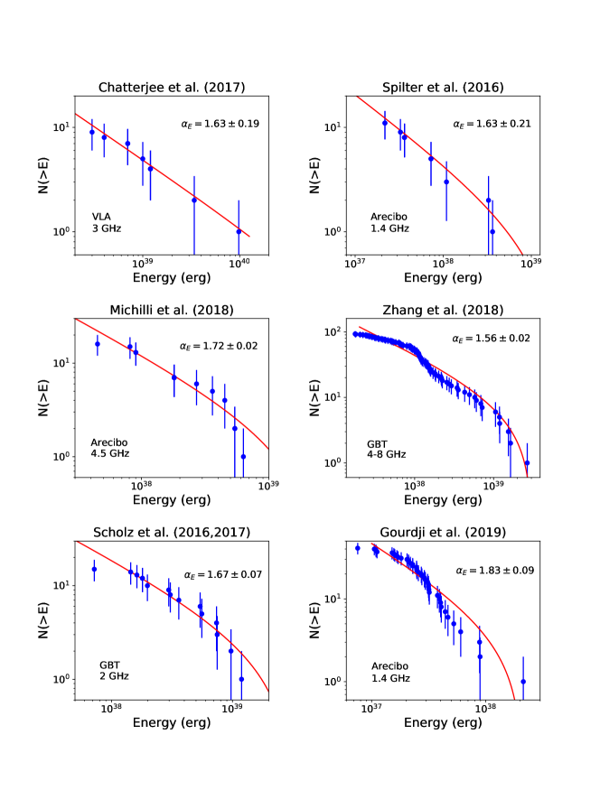
Figure 1: The cumulative energy distributions for different samples of FRB 121102. The observed frequencies and telescopes are shown. The best-fitting power-law index $\alpha_{E}$ for a power-law function with a high energy cut-off (equation (2)) is in a narrow range $1.6<\alpha_{E}<1.8$.

where $E_{\rm max}$ is the maximum energy of FRB and $\alpha_{E}$ is the power-law index of differential distribution $dN/dE\propto E^{-\alpha_{E}}$. Observationally, the high-energy cutoff $E_{\rm max}$ is clearly shown in the samples of Michilli et al. (2018), Scholz et al. (2016), Zhang et al. (2018) and Gourdji et al. (2019) (Figure 1). Theoretically, every astronomical phenomenon must have a maximal energy. Aschwanden (2015) discussed some theoretical reasons for the cutoff, such as contamination by an event-unrelated background and truncation effects at the largest events due to a finite system size. Evidences for the high-energy cutoff have been found in cumulative distributions of solar flares and stellar flares (Aschwanden, 2015), gamma-ray bursts (Wang & Dai, 2013) and soft-gamma repeaters (Prieskorn & Kaaret, 2012). Lu & Kumar (2016) found the maximal luminosity of FRBs under the assumption that FRBs are from coherent curvature emission powered by the dissipation of magnetic energy in the magnetosphere of neutron stars. In addition, due to telescope sensitivity, observational data at low energy may be incomplete, which has been illustrated by Gourdji et al. (2019). Therefore, the completeness threshold at low energy must be considered. We try to fit the cumulative distributions with power-law function in three cases: a power-law function with high-energy cutoff, a power-law function with low-energy threshold and high-energy cutoff, a power-law function with low-energy threshold. The low-energy threshold can be taken into account by omitting bursts below the observational sensitivity. We calculate the sensitivity of VLA at 3 GHz according to Law et al. (2017) and the sensitivity of GBT at 2 GHz according to Scholz et al. (2016). We adopt $2\times 10^{37}$ erg as the sensitivity of Arecibo at 1.4 GHz, which has been used in Gourdji et al. (2019). Using the fluence limit given by Zhang et al. (2018), we calculate the energy limit with the mean bandwidth. Only considering the data with signal-to-noise larger than 5, the energy limit can be derived as $1.02\times 10^{38}$ erg for observation of Arecibo at 4.5 GHz(Michilli et al., 2018). With these sensitivities, we fit the cumulative distributions with an ideal power-law function or a power-law function with cutoff.

The best fitting parameters can be derived by minimizing

$$\chi^{2}=\sum_{i=1}^{n}\frac{\left(N_{ob,i}-N(>E)\right)^{2}}{\sigma_{ob,i}^{2}},$$ (3)

where ${N}_{ob}$ is the number of observed bursts, $N(>E)$ is the model-predicted number of bursts from eq.2 and $\sigma_{ob}$ is the uncertainty of the cumulative distribution. The expected uncertainty of the cumulative distribution is (Aschwanden, 2015)

$$\sigma_{ob,i}=\sqrt{N_{i}}.$$ (4)

We use an open source python package emcee (Foreman-Mackey et al., 2013) to constrain the parameters ($A,\alpha_{E}$ and $E_{\rm max}$) through Markov chain Monte Carlo method. As discussed by Aschwanden (2011) (in page 204 of the book), in reality, there is always a largest event, which causes a gradual steepening in the cumulative frequency distribution, because of the missing contributions up this point. This feature is quite important, because it leads to a significant over-estimate of the power-law slope. The best way is to fit the exact analytical function of the cumulative frequency distribution function $N(>E)=A(E^{1-\alpha_{E}}-E_{\rm max}^{1-\alpha_{E}})$. In our paper, for the cumulative distribution shows obvious steepening in high-energy end, we consider the parameter $E_{\rm max}$ in the fitting. Because the distribution of VLA bursts (Chatterjee et al., 2017) shows ideal power law, the $E_{\rm max}$ is not included in the fitting.

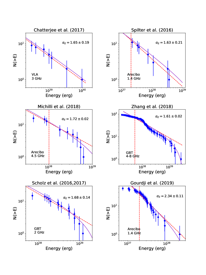
Figure 2: The cumulative energy distributions for different samples of FRB 121102. The observed frequencies and telescopes are shown. The purple solid line is the best fitting by a power-law function with low-energy threshold and high-energy cutoff. The value of $\alpha_{E}$ is for purple solid lines. The red dashed line is the fit by a power-law function with low-energy threshold. The low-energy thresholds are shown as vertical red dashed lines.

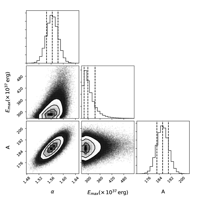
Figure 3: The corner plot of the sample for Zhang et al. (2018).

Figure 1 shows the fitting results of cumulative distributions for different samples with only high-energy cutoff. The best-fitting power-law indices are $\alpha_{E}=1.63\pm 0.19$, $1.63\pm 0.21$, $1.72\pm 0.02$, $1.56\pm 0.02$, $1.67\pm 0.07$ and $1.83\pm 0.09$ for samples from Chatterjee et al. (2017), Spitler et al. (2016), Michilli et al. (2018), Zhang et al. (2018), Scholz et al. (2016, 2017) and Gourdji et al. (2019), respectively. The error represents the $1\sigma$ confidence level. We also list all the best-fitting parameters in Table 1. In these fitting results, the maximal energy is about $200\sim 300\times 10^{37}$ erg except the observations of VLA and the sample of Gourdji et al. (2019). The maximal energy is only $(21\pm 17)\times 10^{37}$ erg for the sample of Gourdji et al. (2019), which is smaller than others. The reason is that the average energy of this sample is lower than others. Besides, through the MCMC method, we also obtain the corner plot of the fitting results. Figure 3 shows the corner plot for samples from Zhang et al. (2018). It is interesting that the value of $\alpha_{E}$ is in a narrow range, i.e., from 1.6 to 1.8. Therefore, a universal energy distribution for FRB 121102 is found. This result is consistent with those of Wang & Yu (2017) and Law et al. (2017). In the other two cases, we show the fitting results in Figure 2 and Table 2. In Figure 2, the purple solid line shows the best fitting with low-energy threshold and high-energy cutoff. The red dashed line represents the best fitting with low-energy threshold, which deviates the observational data at high energies. Therefore, a power-law function can not fit the data by omitting bursts below the observational sensitivity. The high-energy cutoff must be considered. The low-energy sensitivity is shown as vertical red dotted line. From Table 2, we can see that the value of $\alpha_{E}$ is between 1.6 and 1.8, except for the sample of Gourdji et al. (2019). A steeper value $\alpha_{E}=2.8$ is found by Gourdji et al. (2019) using 41 bursts observed Arecibo telescope at 1.4 GHz. This discrepancy may be caused by choosing threshold energy. If these low-energy bursts are considered, the value of $\alpha_{E}$ is around 1.8 (figure 5 of Gourdji et al. (2019)), which is consistent with our result. In addition, the Galactic scintillation also affect the observed radio emission from impulsive radio sources at high frequency (Macquart & Johnston, 2015). For example, the GBT bursts are affected by scintillation at 4-8 GHz, and this complicates calculation of the burst energies (Gajjar et al., 2018; Hessels et al., 2018). Therefore, the fitting result for GBT bursts is not quite well, which is shown in the panel 4 of figure 1.

4 Discussion and Conclusions

In this paper, the energy distribution of the repeating FRB 121102 is studied using six samples observed at different frequencies. We find a universal energy distribution for FRB 121102 with power-law index $1.6<\alpha_{E}<1.8$. However, if low-energy bursts below completeness threshold of Arecibo are discarded for FRB 121102, the slope could be up to 2.3. Some of the implications of our results are as follow.

First, we discuss the volumetric birth rate $R_{FRB}$ of the repeating FRBs. If the life time of each repeater is $\tau$ years, the volume density is $R_{\rm FRB}\tau$. Assuming the formation rate of FRBs tracks the star formation rate (Hopkins & Beacom, 2006), the volumetric birth rate at redshift $z<1$ is $R_{0}(1+z)^{3.28}$, where $R_{0}$ is the local formation rate of FRBs. Considering each repeating FRB has $r(>E_{\rm min})$ pulses with the energy larger than $E_{\rm min}$ per day, we can derive the actual observed rate on sky as

$$\mathcal{R}=\int_{0}^{0.5}\text{d}z\frac{\text{d}V}{\text{d}z}\eta\zeta r({>}E_{min})\frac{R_{0}(1+z)^{3.28}}{(1+z)}\tau,$$ (5)

where $\eta$ is the active duty cycle, $\zeta$ is the beaming effect and $1/(1+z)$ is the effect of the time dilation. According the observation of FRB 121102 (Chatterjee et al., 2017; Zhang et al., 2018), the repeating FRBs are not always active. We introduce $\eta$ to represent the proportion of activate period in the total life and its value is taken as $\eta=0.3$. A typical value $\zeta=0.1$ is taken for beaming effect (Nicholl et al., 2017). We take the cumulative distribution of energy for VLA at 3 GHz as $r(>E_{\rm min})$. The minimum energy in $r(>E_{\rm min})$ can be calculated as $E_{\rm min}=4\pi d_{L}^{2}F_{\rm min}\Delta\nu$, where $F_{\rm min}=0.5$Jy ms is the fluence limit (Scholz et al., 2016). For the observed FRB rate, Cao et al. (2018) estimated $\mathcal{R}>F_{\rm min}\sim 1.4\times 10^{4}$ events per day. Using above information, we obtain $R_{0}\tau\sim 2\times 10^{3}\,\rm{Gpc}^{-3}$. The volume density of repeating FRB sources averaged over $0<z<0.5$ is $R_{\rm FRB}\tau\sim 5\times 10^{3}\,\rm{Gpc}^{-3}$. Lu & Kumar (2019) derived the volume density of repeating FRBs as $\sim 10^{2}-10^{4}\rm{Gpc}^{-3}$, which agrees well with ours. Assuming the luminosity function of repeating FRBs, Nicholl et al. (2017) estimated $R_{\rm FRB}\tau\sim 10^{4}\rm{Gpc}^{-3}$. Considering large uncertainty of FRB rate, ours is marginally consistent their result. Because the possible progenitors of superluminous supernovae (SLSNe), long gamma-ray bursts (LGRBs), short gamma-ray bursts (SGRBs) and repeating FRBs are magnetars (Metzger et al., 2017), we compare their volume rates. For superluminous supernovae, the average rate at $0<z<0.5$ is about $<R_{SLSN}>\sim 40$ Gpc^-3yr^-1 (Quimby et al., 2013). Yu et al. (2015) estimated the rate of LGRB is about $R_{\rm LGRB}=7.2(1+z)^{0.04}$ Gpc^-3yr^-1. Averaging over $0<z<0.5$ and taking their beaming factor of 20 (Fong et al., 2015), we find $<R_{\rm LGRB}>\approx 180$ Gpc^-3yr^-1. Considering the beaming effect, Zhang & Wang (2018) derived the volume rate of SGRB is $<R_{\rm SGRB}>\approx 200$ Gpc^-3yr^-1. If SLSNe and GRBs are the progenitors of millisecond magnetars that power FRBs, observed FRB rates require a lifetime of $\tau\sim 10-100$ years, which is consistent with the estimations of Metzger et al. (2017) and Cao et al. (2017).

Second, we compare our result with the energy distribution for non-repeating FRBs. Lu & Kumar (2019) assumed FRBs are produced by neutron stars at cosmological distances and its rate tracks star formation rate. They found that the observations of non-repeating FRBs are consistent with a universal energy distribution with power-law index $1.5<\alpha_{E}<2.2$, which is consistent with our result. Moreover, the value of $\alpha_{E}$ has a relative small range in our paper. More recently, Zhang & Wang (2019) found the value of $1.6<\alpha_{E}<2.0$ from the cumulative redshift distribution of ASKAP and Parkes samples if the formation rate of FRB has a time delay (3-5 Gyr) relative to cosmic star formation rate. However, if the formation rate of FRB is proportional to the star formation rate, the value of $\alpha_{E}$ is 2.3. So our results support that the central magnetar is formed by merger of binary neutron stars, which is consistent with the large offsets relative to the hist centers of FRB 180924 Bannister et al. (2019) and FRB 190523 Ravi et al. (2019). Lu & Piro (2019) found the value of $\alpha_{E}\sim 1.7$ from the dispersion measurement distribution of ASKAP FRB sample. This value is dramatically consistent with our result. The similar energy distributions between repeating FRB 121102 and non-repeating FRBs may indicate that they share the same underlying physical mechanism (Lu & Piro, 2019).

Third, the energy distributions of other related phenomena are discussed. The giant pulses of Crab show a steeper energy distribution with $\alpha_{E}=2.1-3.5$ (Mickaliger et al., 2012). FRB energy distribution is consistent with magnetar burst ($\alpha_{E}\sim 1.6$; Prieskorn & Kaaret (2012); Wang & Yu (2017)), type I X-ray bursts ($\alpha_{E}\sim 1.5-1.7$; Wang et al. (2017)) and other avalanche events from self-organized criticality systems (Katz, 1986; Bak et al., 1987; Lu & Hamilton, 1991; Aschwanden, 2011; Wang & Dai, 2013; Zhang, Wang & Dai, 2019).

Table 1: The best-fitting results in the high-energy cutoff case.

Telescope	$\alpha_{E}$	$E\_{max}(10^{37}$erg)	A	Reference
VLA at 3 GHz	1.63$\pm 0.19$	-	1.30$\pm 0.37\times 10^{25}$	Chatterjee et al. (2017)
Arecibo at 1.4 GHz	1.83$\pm 0.09$	21$\pm 17$	2.60$\pm 0.12\times 10^{32}$	Gourdji et al. (2019)
Arecibo at 4.5 GHz	1.72$\pm 0.02$	248$\pm 48$	3.01$\pm 0.25\times 10^{28}$	Michilli et al. (2018)
GBT at 2 GHz	1.67$\pm 0.07$	316$\pm 93$	4.58$\pm 0.48\times 10^{26}$	Scholz et al. (2016, 2017)
Arecibo at 1.4 GHz	1.63$\pm 0.21$	204$\pm 90$	4.33$\pm 0.87\times 10^{24}$	Spitler et al. (2016)
GBT at 4-8 GHz	1.56$\pm 0.02$	307$\pm 34$	9.78$\pm 0.21\times 10^{22}$	Zhang et al. (2018)

Table 2: The best-fitting results in the low-energy threshold and high-energy cutoff case, and the low-energy threshold case.

Telescope	$\alpha_{E}$	$\alpha_{E}$	$E_{cut}$($\times 10^{37}$erg)	Reference
VLA at 3 GHz	1.74$\pm 0.03$	1.73$\pm 0.02$	2.31	Chatterjee et al. (2017)
Arecibo at 1.4 GHz	2.34$\pm 0.07$	2.34$\pm 0.11$	2.00	Gourdji et al. (2019)
Arecibo at 4.5 GHz	1.74$\pm 0.03$	1.72$\pm 0.02$	10.24	Michilli et al. (2018)
GBT at 2 GHz	1.76$\pm 0.04$	1.65$\pm 0.07$	4.68	Scholz et al. (2016, 2017)
Arecibo at 1.4 GHz	1.76$\pm 0.15$	1.63$\pm 0.21$	2.00	Spitler et al. (2016)
GBT at 4-8 GHz	1.69$\pm 0.01$	1.61$\pm 0.02$	5.27	Zhang et al. (2018)

Table 3: The VLA observation at 3 GHz from Chatterjee et al.(2017).

MJD	Fluence (Jy ms)	Central Frequency (GHz)	Bandwidth (MHz)	Width (ms)	Energy ($10^{38}$ erg)
57623.74402	-	2.80	290	2.00	12
57633.67986	-	3.20	510	2.05	98
57633.69516	-	<2.50	<290	2.50	7
57638.49937	-	3.10	420	1.30	3
57643.45730	-	2.80	510	1.90	34
57645.42959	-	2.80	380	1.10	4
57646.43691	-	<2.50	<430	2.50	10
57648.43691	-	2.80	470	1.40	7
57649.45176	-	3.00	690	2.10	12

Table 4: The Arecibo observation at 1.4 GHz from Gourdji et al. (2019).

MJD	Fluence (Jy ms)	Central Frequency (GHz)	Bandwidth (MHz)	Width (ms)	Energy ($10^{38}$ erg)
57644.41107	0.80	1.40	237	1.99	2.14
57644.41412	0.11	1.64	176	5.40	0.22
57644.41488	0.09	1.54	244	2.60	0.25
57644.41631	0.14	1.67	115	4.20	0.18
57644.43017	0.09	1.68	104	2.40	0.11
57644.43017	0.16	1.65	151	4.40	0.27
57644.43224	0.11	1.69	90	1.50	0.11
57644.43879	0.19	1.49	218	5.10	0.47
57644.43884	0.15	1.40	152	5.60	0.26
57644.44359	0.07	1.41	211	2.10	0.17
57644.44679	0.03	1.57	324	0.73	0.11
57644.44773	0.40	1.38	55	6.00	0.25
57644.44991	0.07	1.66	138	2.00	0.11
57644.45160	0.22	1.67	128	3.30	0.32
57644.45448	0.60	1.36	132	9.10	0.89
57644.45788	0.03	1.40	239	1.10	0.08
57644.46622	0.20	1.66	131	4.20	0.30
57644.46809	0.21	1.66	133	7.70	0.31
57645.41109	0.20	1.53	392	1.78	0.88
57645.41165	0.17	1.45	144	3.70	0.28
57645.41364	0.13	1.60	268	4.30	0.39
57645.41747	0.08	1.43	177	4.70	0.16
57645.41790	0.09	1.65	168	2.40	0.17
57645.42026	0.24	1.37	194	13.50	0.52
57645.42245	0.13	1.62	215	3.80	0.32
57645.42414	0.08	1.60	255	4.00	0.23
57645.42890	0.14	1.49	280	8.20	0.44
57645.43062	0.09	1.63	208	2.80	0.21
57645.43148	0.09	1.66	149	1.90	0.15
57645.44081	0.22	1.67	117	3.00	0.29
57645.44448	0.10	1.66	139	2.10	0.16
57645.44492	0.25	1.46	134	6.10	0.38
57645.44764	0.17	1.39	110	4.00	0.21
57645.44880	0.14	1.47	196	1.47	0.31
57645.44999	0.24	1.43	223	9.20	0.60
57645.44999	0.12	1.65	151	2.40	0.20
57645.45343	0.20	1.44	142	2.80	0.32
57645.45364	0.30	1.67	119	6.20	0.40
57645.46211	0.27	1.38	134	7.00	0.41
57645.46419	0.09	1.62	226	3.70	0.23
57645.47445	0.17	1.67	130	4.80	0.25

Table 5: The Arecibo observation at 4.5 GHz from Michilli et al. (2018).

MJD	Fluence (Jy ms)	Central Frequency (GHz)	Bandwidth (MHz)	Width (ms)	Energy ($10^{38}$ erg)
57747.12956	0.70	4.50	800	0.80	6.31
57747.13719	0.20	4.50	800	0.85	1.80
57747.14627	0.20	4.50	800	0.22	1.80
57747.15157	0.09	4.50	800	0.55	0.81
57747.15447	0.10	4.50	800	0.76	0.90
57747.16029	0.05	4.50	800	0.03	0.45
57747.16034	0.20	4.50	800	0.31	1.80
57747.16583	0.50	4.50	800	1.36	4.51
57747.16637	0.30	4.50	800	1.92	2.70
57747.17597	0.20	4.50	800	0.98	1.80
57748.12564	0.10	4.50	800	0.95	0.90
57748.15352	0.20	4.50	800	0.42	1.80
57748.15521	0.60	4.50	800	0.78	5.41
57748.15761	0.20	4.50	800	0.15	1.80
57748.17570	0.40	4.50	800	0.54	3.61
57772.12903	0.60	4.50	800	0.74	5.41

Table 6: The GBT observation at 2 GHz from Scholz et al. (2016).

MJD	Fluence (Jy ms)	Central Frequency (GHz)	Bandwidth (MHz)	Width (ms)	Energy ($10^{38}$ erg)
57339.35605	0.20	2.00	800	6.73	1.80
57345.44769	0.40	2.00	800	6.10	3.61
57345.45249	0.20	2.00	800	6.14	1.80
57345.45760	0.08	2.00	800	4.30	0.72
57345.46241	0.60	2.00	800	5.97	5.41
57647.23235	0.82	2.00	800	2.16	7.39
57647.23235	0.16	2.00	800	1.94	1.44
57649.17381	1.32	2.00	800	3.45	11.90
57649.21821	0.34	2.00	800	0.88	3.07
57765.04953	0.33	2.00	800	1.40	2.98
57765.06479	0.83	2.00	800	1.79	7.48
57765.06905	0.62	2.00	800	2.97	5.59
57765.10083	0.18	2.00	800	2.46	1.62
57765.12078	1.08	2.00	800	1.36	9.74
57765.13650	0.22	2.00	800	1.68	1.98

Table 7: The Arecibo observation at 1.4 GHz from Spilter et al. (2016).

MJD	Fluence (Jy ms)	Central Frequency (GHz)	Bandwidth (MHz)	Width (ms)	Energy ($10^{38}$ erg)
56233.28284	0.10	1.40	322	3.30	0.36
57159.73760	0.10	1.40	322	3.80	0.36
57159.74422	0.10	1.40	322	3.30	0.36
57175.69314	0.20	1.40	322	4.60	0.73
57175.69973	0.09	1.40	322	8.70	0.33
57175.74258	0.06	1.40	322	2.80	0.22
57175.74284	0.06	1.40	322	6.10	0.22
57175.74351	0.90	1.40	322	6.60	3.27
57175.74567	0.30	1.40	322	6.00	1.09
57175.74762	0.20	1.40	322	8.00	0.73
57175.74829	1.00	1.40	322	3.06	3.63

Table 8: The GBT observation at 4-8 GHz from Zhang et al. (2018).

MJD	Fluence (Jy ms)	Central Frequency (GHz)	Bandwidth (MHz)	Width (ms)	Energy ($10^{38}$ erg)
57991.4099	0.61	6.05	3900	1.43	26.64
57991.40993	0.03	6.75	2300	2.15	0.66
57991.41002	0.05	6.3	2400	1.43	1.37
57991.41007	0.09	6.25	2500	2.51	2.55
57991.41156	0.05	6.25	2500	1.79	1.49
57991.41209	0.04	5.7	1400	1.79	0.69
57991.41231	0.03	6.3	2400	1.08	0.71
57991.41276	0.07	5.95	3900	1.43	2.92
57991.41276	0.07	5.45	2900	1.79	2.20
57991.41293	0.15	6	3000	3.58	4.94
57991.41302	0.06	7	1800	0.72	1.15
57991.41336	0.05	7	1800	1.43	0.95
57991.41346	0.36	6	4000	1.08	16.37
57991.41371	0.26	6	4000	1.08	11.85
57991.41384	0.26	6	4000	1.43	11.93
57991.41613	0.04	6.05	2900	1.79	1.15
57991.41619	0.05	6.3	2400	1.79	1.25
57991.41621	0.02	5.5	2000	1.08	0.52
57991.41644	0.04	5.95	3900	1.08	1.59
57991.41663	0.35	6.05	3900	1.08	15.35
57991.41727	0.05	6.25	2500	1.08	1.48
57991.41738	0.03	5.95	1900	0.72	0.63
57991.41771	0.04	6.25	2500	1.08	0.99
57991.41787	0.08	6.05	3900	1.08	3.56
57991.41863	0.1	6.05	3900	1.43	4.30
57991.41903	0.04	6	2000	1.43	0.90
57991.41945	0.04	5.85	1700	1.43	0.85
57991.41945	0.02	7.1	1000	1.08	0.24
57991.41945	0.04	5.9	1600	1.08	0.65
57991.41946	0.03	5.5	2000	1.79	0.58
57991.41946	0.03	5.55	1900	1.43	0.63
57991.42087	0.03	7.15	1300	1.43	0.42
57991.42121	0.06	6	4000	0.72	2.74
57991.42171	0.08	5.95	3900	0.72	3.45
57991.42212	0.07	5.5	2000	1.79	1.54
57991.42214	0.04	6.7	2400	1.79	1.07
57991.42294	0.13	6.05	3900	1.79	5.77
57991.42301	0.03	6	4000	2.15	1.19
57991.42427	0.05	5.55	1900	1.79	1.13
57991.42454	0.02	5.05	900	1.08	0.18
57991.42592	0.03	5.55	900	2.15	0.29
57991.42639	0.07	6.05	1900	2.15	1.44
57991.42655	0.16	6.05	3900	0.72	6.88
57991.42839	0.07	6.7	2400	2.51	2.02
57991.42859	0.04	5.95	3900	1.08	1.59
57991.43043	0.05	5.95	3900	1.08	2.24
57991.4311	0.06	6.2	1400	3.23	0.91
57991.43167	0.04	6	2000	1.79	0.93
57991.43197	0.16	5.95	3900	1.08	7.16
57991.43228	0.05	6	2000	1.43	1.08
57991.43484	0.02	6.45	1900	1.79	0.52
57991.4352	0.06	6.55	1900	1.43	1.20
57991.43656	0.06	6.95	1900	1.08	1.21
57991.43785	0.02	6.7	2400	1.08	0.66
57991.43849	0.02	5.75	1500	1.08	0.38
57991.43936	0.23	6	4000	1.79	10.56
57991.44621	0.02	6.2	1400	0.72	0.28
57991.44699	0.01	6.25	1500	0.72	0.22
57991.44793	0.05	5.95	2900	2.51	1.71
57991.44805	0.03	4.95	900	2.15	0.26
57991.44843	0.14	5.95	3900	1.08	6.04
57991.45018	0.02	5.3	1400	0.72	0.31
57991.45047	0.03	6.75	2300	1.43	0.89
57991.45304	0.07	5.7	2400	1.43	1.82
57991.45851	0.02	5.3	1400	1.79	0.34
57991.46087	0.03	7.2	1400	1.08	0.43
57991.46371	0.05	6.25	1900	1.08	1.01
57991.46394	0.04	5.5	2000	1.43	0.99
57991.46394	0.04	6	3000	1.08	1.24
57991.47019	0.02	5.8	1400	0.72	0.32
57991.47115	0.03	6.25	1500	2.15	0.46
57991.47287	0.02	5.05	900	1.79	0.20
57991.48003	0.04	5.5	2000	1.79	0.79
57991.4886	0.03	6.45	900	2.87	0.27
57991.49316	0.02	5.45	1900	1.79	0.40
57991.49751	0.05	5.5	2000	1.43	1.13
57991.49839	0.02	5.55	900	2.15	0.25
57991.49882	0.05	5.7	2400	1.79	1.39
57991.51086	0.02	6.5	2000	0.72	0.54
57991.51311	0.1	5.5	2000	1.08	2.17
57991.51923	0.05	6.5	2000	2.87	1.12
57991.51923	0.07	6.5	2000	1.43	1.49
57991.5594	0.03	6.05	3900	0.72	1.31
57991.56282	0.06	6.5	2800	1.08	1.85
57991.56945	0.07	5.5	2000	2.87	1.57
57991.571	0.05	5.55	1900	1.43	1.05
57991.57444	0.02	6.45	900	2.51	0.18
57991.58815	0.05	5.5	2000	1.08	1.08
57991.59051	0.04	6.3	2400	1.08	1.14
57991.59211	0.05	6	2000	1.08	1.17
57991.59543	0.02	6.25	1500	0.72	0.35
57991.59576	0.03	6.25	1500	1.43	0.49
57991.60226	0.02	5.15	1300	0.72	0.31

References

- Aschwanden (2011) Aschwanden, M. J. 2011, Self-Organized Criticality Astrophysics: The Statistics of Nonlinear Processes in the Universe (Berlin: Springer)
- Aschwanden (2015) Aschwanden, M. J. 2015, ApJ, 814, 19
- Bak et al. (1987) Bak, P., Tang, C., & Wiesenfeld, K. 1987, Phys. Rev. Lett., 59, 381
- Bannister et al. (2019) Bannister, K. W., et al., 2019, Science, 10.1126/science.aaw5903
- Caleb et al. (2018) Caleb, M., Spitler, L. G. & Stappers, B. W., 2018, Nature Astronomy, 2, 839
- Cao et al. (2017) Cao, X.-F., Yu, Y.-W., & Dai, Z. G. 2017, ApJ, 839, L20
- Cao et al. (2018) Cao, X.-F., Yu, Y.-W., & Zhou, X. 2018, ApJ, 858, 89
- Chatterjee et al. (2017) Chatterjee, S., Law, C. J., Wharton, R. S., et al. 2017, Nature, 541, 58
- CHIME/FRB Collaboration et al. (2019) CHIME/FRB Collaboration, Amiri, M., Bandura, K., et al. 2019, Nature, 566, 235
- Deng & Zhang (2014) Deng, W., & Zhang, B. 2014, ApJ, 783, L35
- Hopkins & Beacom (2006) Hopkins, A. M., & Beacom, J. F. 2006, ApJ, 651, 142
- Fong et al. (2015) Fong, W., Berger, E., Margutti, R., et al. 2015, ApJ, 815, 102
- Foreman-Mackey et al. (2013) Foreman-Mackey, D., Hogg, D. W., Lang, D., et al. 2013, PASP, 125, 306
- Gajjar et al. (2018) Gajjar, V., Siemion, A. P. V., Price, D. C., et al. 2018, ApJ, 863, 2
- Gao et al. (2014) Gao, H., Li, Z., & Zhang, B. 2014, ApJ, 788, 189
- Gourdji et al. (2019) Gourdji, K., Michilli, D., Spitler, L. G., et al. 2019, ApJL, 877, L19
- Hessels et al. (2018) Hessels, J. W. T., Spitler, L. G., Seymour, A. D., et al. 2018, arXiv:1811.10748
- Katz (1986) Katz, J. I. 1986, J. Geophys. Res., 91, 10412
- Katz (2016) Katz, J. I. 2016, ApJ, 826, 226
- Keane & Petroff (2015) Keane, E. F., & Petroff, E. 2015, MNRAS, 447, 2852
- Law et al. (2017) Law, C. J., Abruzzo, M. W., Bassa, C. G., et al. 2017, ApJ, 850, 76
- Li et al. (2017) Li, L.-B., Huang, Y.-F., Zhang, Z.-B., et al. 2017, RAA, 17, 6
- Li et al. (2018) Li, Z.-X., Gao, H., Ding, X.-H., et al. 2018, Nature Communications, 9, 3833
- Li et al. (2019) Li, Z.-X., et al. 2019, arXiv: 1904.08927
- Lorimer et al. (2007) Lorimer, D. R., Bailes, M., McLaughlin, M. A., et al. 2007, Science, 318, 777
- Lu & Hamilton (1991) Lu, E. T., & Hamilton, R. J. 1991, ApJ, 380, L89
- Lu & Kumar (2016) Lu, W., & Kumar, P. 2019, MNRAS, 483, L93
- Lu & Kumar (2019) Lu, W., & Kumar, P. 2016, MNRAS, 461, L122
- Lu & Piro (2019) Lu, W., & Piro, A. L. 2019, arXiv e-prints , arXiv:1903.00014
- Luo et al. (2018) Luo, R., Lee, K., Lorimer, D. R., et al. 2018, MNRAS, 481, 2320
- Macquart & Johnston (2015) Macquart, J.-P., & Johnston, S. 2015, MNRAS, 451, 3278
- Macquart & Ekers (2018) Macquart, J.-P., & Ekers, R. 2018, MNRAS, 480, 4211
- Macquart (2018) Macquart, J.-P. 2018, Nature Astronomy, 2, 836
- McQuinn (2014) McQuinn, M. 2014, ApJ, 780, L33
- Metzger et al. (2017) Metzger, B. D., Berger, E. & Margalit, B., 2017, ApJ, 841, 14
- Michilli et al. (2018) Michilli, D., Seymour, A., Hessels, J. W. T., et al. 2018, Nature, 553, 182
- Mickaliger et al. (2012) Mickaliger, M. B., McLaughlin, M. A., Lorimer, D. R., et al. 2012, ApJ, 760, 64
- Nicholl et al. (2017) Nicholl, M., Williams, P. K. G., Berger, E., et al. 2017, ApJ, 843, 84
- Palaniswamy et al. (2018) Palaniswamy, D., Li, Y. & Zhang, B., 2018, ApJ, 854, L12
- Pen (2018) Pen, U.-L. 2018, Nature Astronomy, 2, 842
- Petroff et al. (2016) Petroff, E., Barr, E. D., Jameson, A., et al. 2016, PASA, 33, e045
- Prieskorn & Kaaret (2012) Prieskorn, Z., & Kaaret, P. 2012, ApJ, 755, 1
- Quimby et al. (2013) Quimby, R. M., Yuan, F., Akerlof, C., & Wheeler, J. C. 2013, MNRAS, 431, 912
- Ravi (2019) Ravi, V. 2019, MNRAS, 482, 1966
- Ravi et al. (2019) Ravi, V., et al., 2019, Nature, doi:10.1038/s41586-019-1389-7
- Scholz et al. (2016) Scholz, P., Spitler, L. G., Hessels, J. W. T., et al. 2016, ApJ, 833, 177
- Scholz et al. (2017) Scholz, P., Bogdanov, S., Hessels, J. W. T., et al. 2017, ApJ, 846, 80
- Spitler et al. (2014) Spitler, L. G., Cordes, J. M., Hessels, J. W. T., et al. 2014, ApJ, 790, 101
- Spitler et al. (2016) Spitler, L. G., Scholz, P., Hessels, J. W. T., et al. 2016, Nature, 531, 202
- Spitler et al. (2018) Spitler, L. G., Herrmann, W., Bower, G. C., et al. 2018, ApJ, 863, 150
- Thornton et al. (2013) Thornton, D., Stappers, B., Bailes, M., et al. 2013, Science, 341, 53
- Walters et al. (2018) Walters, A., Weltman, A., Gaensler, B. M., et al. 2018, ApJ, 856, 65
- Wang & Dai (2013) Wang, F. Y., & Dai, Z. G. 2013, Nature Physics, 9, 465
- Wang & Yu (2017) Wang, F. Y., & Yu, H. 2017, JCAP, 2017, 23
- Wang et al. (2017) Wang, J. S., Wang, F. Y., & Dai, Z. G. 2017, MNRAS, 471, 2517
- Wang & Wang (2018) Wang, Y. K., & Wang, F. Y. 2018, A&A, 614, A50
- Wei et al. (2015) Wei, J.-J., Gao, H., Wu, X.-F., et al. 2015, Phys. Rev. Lett., 115, 261101
- Yang & Zhang (2016) Yang, Y.-P., Zhang, B. 2016, ApJ, 830, L31
- Yu et al. (2015) Yu, H., Wang, F. Y., Dai, Z. G., et al. 2015, ApJS, 218, 13
- Yu & Wang (2017) Yu, H., & Wang, F. Y. 2017, A&A, 606, A3
- Zhang & Wang (2018) Zhang, G. Q., & Wang, F. Y. 2018, ApJ, 852, 1
- Zhang, Wang & Dai (2019) Zhang, G. Q., Wang, F. Y., & Dai, Z. G. 2019, arXiv e-prints, arXiv:1903.11895
- Zhang & Wang (2019) Zhang, G. Q. & Wang, F. Y., 2019, MNRAS, 487, 3672
- Zhang et al. (2018) Zhang, Y. G., Gajjar, V., Foster, G., et al. 2018, ApJ, 866, 149
- Zheng et al. (2014) Zheng, Z., Ofek, E. O., Kulkarni, S. R., et al. 2014, ApJ, 797, 71
- Zhou et al. (2014) Zhou, B., Li, X., Wang, T., et al. 2014, Phys. Rev. D, 89, 107303