Adversarial Speaker Adaptation

Abstract

We propose a novel adversarial speaker adaptation (ASA) scheme, in which adversarial learning is applied to regularize the distribution of deep hidden features in a speaker-dependent (SD) deep neural network (DNN) acoustic model to be close to that of a fixed speaker-independent (SI) DNN acoustic model during adaptation. An additional discriminator network is introduced to distinguish the deep features generated by the SD model from those produced by the SI model. In ASA, with a fixed SI model as the reference, an SD model is jointly optimized with the discriminator network to minimize the senone classification loss, and simultaneously to mini-maximize the SI/SD discrimination loss on the adaptation data. With ASA, a senone-discriminative deep feature is learned in the SD model with a similar distribution to that of the SI model. With such a regularized and adapted deep feature, the SD model can perform improved automatic speech recognition on the target speaker’s speech. Evaluated on the Microsoft short message dictation dataset, ASA achieves 14.4% and 7.9% relative word error rate improvements for supervised and unsupervised adaptation, respectively, over an SI model trained from 2600 hours data, with 200 adaptation utterances per speaker.

Index Terms—  adversarial learning, speaker adaptation, neural network, automatic speech recognition

1 Introduction

With the advent of deep learning, the performance of automatic speech recognition (ASR) has greatly improved [1, 2]. However, the ASR performance is not optimal when acoustic mismatch exists between training and testing [3]. Acoustic model adaptation is a natural solution to compensate for this mismatch. For speaker adaptation, we are given a speaker-independent (SI) acoustic model that performs reasonably well on the speech of almost all speakers in general. Our goal is to learn a personalized speaker-dependent (SD) acoustic model for each target speaker that achieves optimal ASR performance on his/her own speech. This is achieved by adapting the SI model to the speech of each target speaker.

The speaker adaptation task is more challenging than the other types of domain adaptation tasks in that it has only access to very limited adaptation data from the target speaker and has no access to the source domain data, e.g. speech from other general speakers. Moreover, a deep neural network (DNN) based SI model, usually with a large number of parameters, can easily get overfitted to the limited adaptation data. To address this issue, transformation-based approaches are introduced in [4, 5] to reduce the number of learnable parameters by inserting a linear network to the input, output or hidden layers of the SI model. In [6, 7], the trainable parameters are further reduced by singular value decomposition (SVD) of weight matrices of a neural network and perform adaptation on an inserted square matrix between the two low-rank matrices. Moreover, i-vector [8] and speaker-code [9, 10] are widely used as auxiliary features to a neural network for speaker adaptation. Further, regularization-based approaches are proposed in [11, 12, 13, 14] to regularize the neuron output distributions or the model parameters of the SD model such that it does not stray too far away from the SI model.

In this work, we propose a novel regularization-based approach for speaker adaptation, in which we use adversarial multi-task learning (MTL) to regularize the distribution of the deep features (i.e., hidden representations) in an SD DNN acoustic model such that it does not deviate too much from the deep feature distribution in the SI DNN acoustic model. We call this method adversarial speaker adaptation (ASA). Recently, adversarial training has achieved great success in learning generative models [15]. In speech area, it has been applied to acoustic model adaptation [16, 17], noise-robust [18, 19, 20], speaker-invariant [21, 22, 23] ASR, speech enhancement [24, 25, 26] and speaker verification [27, 28] using gradient reversal layer [29] or domain separation network [30]. In these works, adversarial MTL assists in learning a deep intermediate feature that is both senone-discriminative and domain-invariant.

In ASA, we introduce an auxiliary discriminator network to classify whether an input deep feature is generated by an SD or SI acoustic model. By using a fixed SI acoustic model as the reference, the discriminator network is jointly trained with the SD acoustic model to simultaneously optimize the primary task of minimizing the senone classification loss and the secondary task of mini-maximizing the SD/SI discrimination loss on the adaptation data. Through this adversarial MTL, senone-discriminative deep features are learned in the SD model with a distribution that is similar to that of the SI model. With such a regularized and adapted deep feature, the SD model is expected to achieve improved ASR performance on the test speech from the target speaker. As an extension, ASA can also be performed on the senone posteriors (ASA-SP) to regularize the output distribution of the SD model.

We perform speaker adaptation experiments on Microsoft short message (SMD) dictation dataset with 2600 hours of live US English data for training. ASA achieves up to 14.4% and 7.9% relative word error rate (WER) improvements for supervised and unsupervised adaptation, respectively, over an SI model trained on 2600 hours of speech.

2 Adversarial Speaker Adaptation

In speaker adaptation task, for a target speaker, we are given a sequence of adaptation speech frames $\mathbf{X}=\{\mathbf{x}_{1},\ldots,\mathbf{x}_{T}\},\mathbf{x}_{t}\in\mathbbm{R}^{r_{x}},t=1,\ldots,T$ from the target speaker and a sequence of senone labels $\mathbf{Y}=\{y_{1},\ldots,y_{T}\},y_{t}\in\mathbbm{R}$ aligned with $\mathbf{X}$. For supervised adaptation, $\mathbf{Y}$ is generated by aligning the adaptation data against the transcription using SI acoustic model while for unsupervised adaptation, the adaptation data is first decoded using the SI acoustic model and the one-best path of the decoding lattice is used as $\mathbf{Y}$.

As shown in Fig. 1, we view the first few layers of a well-trained SI DNN acoustic model as an SI feature extractor network $M_{f}^{\text{SI}}$ with parameters $\theta_{f}^{\text{SI}}$ and the the upper layers of the SI model as an SI senone classifier network $M_{y}^{\text{SI}}$ with parameters $\theta_{y}^{\text{SI}}$. $M_{f}^{\text{SI}}$ maps input adaptation speech frames $\mathbf{X}$ to intermediate SI deep hidden features $\mathbf{F}^{\text{SI}}=\{\mathbf{f}_{1}^{\text{SI}},\ldots,\mathbf{f}_{T}^{\text{SI}}\},\mathbf{f}_{t}^{\text{SI}}\in\mathbbm{R}^{r_{f}}$, i.e.,

$$\mathbf{f}_{t}^{\text{SI}}=M_{f}^{\text{SI}}(\mathbf{x}_{t}),$$ (1)

and $M_{y}^{\text{SI}}$ with parameters $\theta_{y}^{\text{SI}}$ maps $\mathbf{F}^{\text{SI}}$ to the posteriors $p(s|\mathbf{f}_{t}^{\text{SI}};\theta_{y}^{\text{SI}})$ of a set of senones in $\mathbbm{S}$ as follows:

$$M_{y}^{\text{SI}}(\mathbf{f}_{t}^{\text{SI}})=p(s|\mathbf{x}_{t};\mathbf{\theta}^{\text{SI}}_{f},\mathbf{\theta}^{\text{SI}}_{y}).$$ (2)

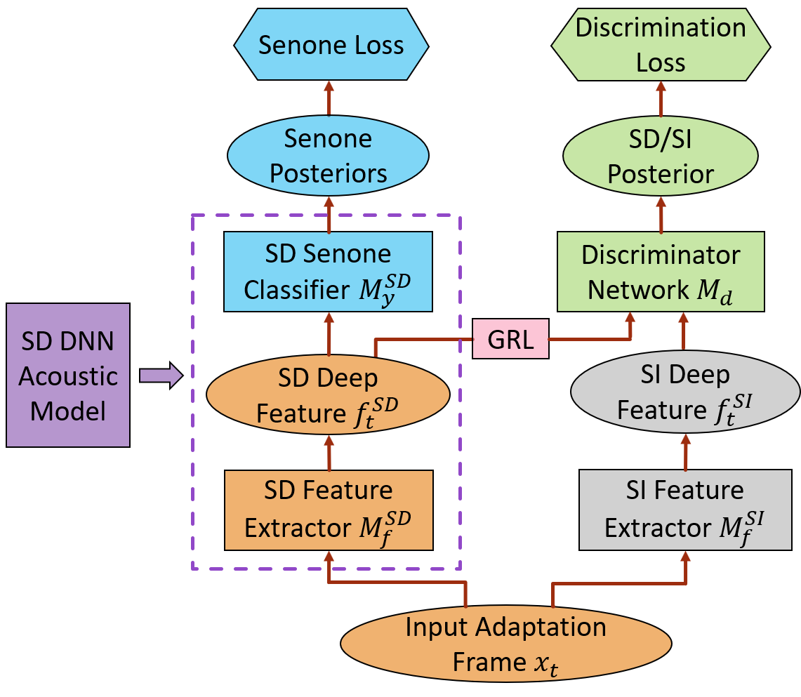
Fig. 1: The framework of ASA. Only the optimized SD acoustic model consisting of $M_{f}^{\text{SD}}$ and $M_{y}^{\text{SD}}$ are used for ASR on test data. $M_{f}^{\text{SI}}$ is fixed during ASA. $M_{f}^{\text{SI}}$ and $M_{d}$ are discarded after ASA.

An SD DNN acoustic model to be trained using speech from the target speaker is initialized from the SI acoustic model. Specifically, $M_{f}^{\text{SI}}$ is used to initialize SD feature extractor $M_{f}^{\text{SD}}$ with parameters $\theta_{f}^{\text{SD}}$ and $M_{y}^{\text{SI}}$ is used to initialize SD senone classifier $M_{y}^{\text{SD}}$ with parameters $\theta_{y}^{\text{SD}}$. Similarly, in an SD model, $M_{f}^{\text{SD}}$ maps $\mathbf{x}_{t}$ to SD deep features $\mathbf{f}_{t}^{\text{SD}}$ and $M_{y}^{\text{SD}}$ further transforms $\mathbf{f}_{t}^{\text{SD}}$ to the same set of senone posteriors $p(s|\mathbf{f}_{t}^{\text{SD}};\theta_{y}^{\text{SD}}),s\in\mathbbm{S}$ as follows

$$M_{y}^{\text{SD}}(\mathbf{f}_{t}^{\text{SD}})=M_{y}^{\text{SD}}(M_{f}^{\text{SD}}(\mathbf{x}_{t}))=p(s|\mathbf{x}_{t};\mathbf{\theta}^{\text{SD}}_{f},\mathbf{\theta}^{\text{SD}}_{y}).$$ (3)

To adapt the SI model to target speech $\mathbf{X}$, we re-train the SD model by minimizing the cross-entropy senone classification loss between the predicted senone posteriors and the senone labels $\mathbf{Y}$ below

$$\mathcal{L}_{\text{senone}}(\theta_{f}^{\text{SD}},\theta_{y}^{\text{SD}})=-\frac{1}{T}\sum_{t=1}^{T}\log p(y_{t}|\mathbf{x}_{t};\theta_{f}^{\text{SD}},\theta_{y}^{\text{SD}})$$

$$\qquad\quad=-\frac{1}{T}\sum_{t=1}^{T}\sum_{s\in\mathbbm{S}}\mathbbm{1}[s=y_{t}]\log M_{y}(M_{f}^{\text{SD}}(\mathbf{x}_{t})),$$ (4)

where $\mathbbm{1}[\cdot]$ is the indicator function which equals to 1 if the condition in the squared bracket is satisfied and 0 otherwise.

However, the adaptation data $\mathbf{X}$ is usually very limited for the target speaker and the SI model with a large number of parameters can easily get overfitted to the adaptation data. Therefore, we need to force the distribution of deep hidden features $\mathbf{F}^{\text{SD}}$ in the SD model to be close to that of the deep features $\mathbf{F}^{\text{SI}}$ in SI model while minimizing $\mathcal{L}_{\text{senone}}$ as follows

$$p({\mathbf{F}^{\text{SD}}}|\mathbf{X},\theta_{f}^{\text{SD}})\rightarrow p({\mathbf{F}^{\text{SI}}}|\mathbf{X},\theta_{f}^{\text{SI}}),$$ (5)

$$\min_{\theta_{f}^{\text{SD}},\theta_{y}^{\text{SD}}}\mathcal{L}_{\text{senone}}(\theta_{f}^{\text{SD}},\theta_{y}^{\text{SD}}).$$ (6)

In KLD adaptation [11], the senone distribution estimated from the SD model is forced to be close to that estimated from an SI model by adding a KLD regularization to the adaptation criterion. However, KLD is a distribution-wise asymmetric measure which does not serve as a perfect distance metric between distributions [31]. For example, in [11], the minimization of $\mathcal{KL}(p^{\text{SI}}||p^{\text{SD}})$ does not guarantee $\mathcal{KL}(p^{\text{SD}}||p^{\text{SI}})$ is also minimized. In some cases, $\mathcal{KL}(p^{\text{SD}}||p^{\text{SI}})$ even increases as $\mathcal{KL}(p^{\text{SI}}||p^{\text{SD}})$ becomes smaller [32, 33]. In ASA, we use adversarial MTL instead to push the distribution of $\mathbf{F}^{\text{SD}}$ towards that of $\mathbf{F}^{\text{SI}}$ while being adapted to the target speech since the adversarial learning can guarantee that the global optimum is achieved if and only if $\mathbf{F}^{\text{SD}}$ and $\mathbf{F}^{\text{SI}}$ share exactly the same distribution [15].

To achieve Eq. (5), we introduce an additional discriminator network $M_{d}$ with parameters $\theta_{d}$ which takes $\mathbf{F}^{\text{SD}}$ and $\mathbf{F}^{\text{SI}}$ as the input and outputs the posterior probability that an input deep feature is generated by the SD model, i.e.,

$$M_{d}(\mathbf{f}_{t}^{\text{SD}}) =p(\mathbf{f}_{t}^{\text{SD}}\in\mathbbm{D}_{\text{SD}}|\mathbf{x}_{t};\theta^{\text{SD}}_{f},\theta_{d}),$$ (7)

$$M_{d}(\mathbf{f}_{t}^{\text{SI}}) =1-p(\mathbf{f}_{t}^{\text{SI}}\in\mathbbm{D}_{\text{SI}}|\mathbf{x}_{t};\theta^{\text{SI}}_{f},\theta_{d}),$$ (8)

where $\mathbbm{D}_{\text{SD}}$ and $\mathbbm{D}_{\text{SI}}$ denote the sets of SD and SI deep features, respectively. The discrimination loss $\mathcal{L}_{\text{disc}}(\theta_{f},\theta_{d})$ for $M_{d}$ is formulated below using cross-entropy:

$$\mathcal{L}_{\text{disc}}(\theta^{\text{SD}}_{f},\theta^{\text{SI}}_{f},\theta_{d})=-\frac{1}{T}\sum_{t=1}^{T}\left[\log p(\mathbf{f}_{t}^{\text{SD}}\in\mathbbm{D}_{\text{SD}}|\mathbf{x}_{t};\theta^{\text{SD}}_{f},\theta_{d})\right.$$

$$\qquad\qquad\qquad\qquad\qquad\quad\left.+\log p(\mathbf{f}_{t}^{\text{SI}}\in\mathbbm{D}_{\text{SI}}|\mathbf{x}_{t};\theta^{\text{SI}}_{f},\theta_{d})\right]$$

$$=-\frac{1}{T}\sum_{t=1}^{T}\left\{\log M_{d}(M_{f}^{\text{SD}}(\mathbf{x}_{t}))+\log\left[1-M_{d}(M_{f}^{\text{SI}}(\mathbf{x}_{t}))\right]\right\}$$ (9)

To make the distribution of $\mathbf{F}^{\text{SD}}$ similar to that of $\mathbf{F}^{\text{SI}}$, we perform adversarial training of $M_{f}^{\text{SD}}$ and $M_{d}$, i.e, we minimize $\mathcal{L}_{\text{disc}}$ with respect to $\theta_{d}$ and maximize $\mathcal{L}_{\text{disc}}$ with respect to $\theta^{\text{SD}}_{f}$. This minimax competition will first increase the capability of $M_{f}^{\text{SD}}$ to generate $\mathbf{F}^{\text{SD}}$ with a distribution similar to that of $\mathbf{F}^{\text{SI}}$ and increase the discrimination capability of $M_{d}$. It will eventually converge to the point where $M_{f}^{\text{SD}}$ generates extremely confusing $\mathbf{F}^{\text{SD}}$ that $M_{d}$ is unable to distinguish whether it is generated by $M_{f}^{\text{SD}}$ or $M_{f}^{\text{SI}}$. At this point, we have successfully regularized the SD model such that it does not deviate too much from the SI model and generalizes well to the test speech from target speaker.

With ASA, we want to learn a senone-discriminative SD deep feature with a similar distribution to the SI deep features as in Eq. (5) and (6). To achieve this, we perform adversarial MTL, in which the SD model and $M_{d}$ are trained to jointly optimize the primary task of senone classification and the secondary task of SD/SI discrimination with an adversarial objective function as follows

$$(\hat{\mathbf{\theta}}_{f}^{\text{SD}},\hat{\mathbf{\theta}}_{y}^{\text{SD}}) =\operatorname*{arg\,min}_{\mathbf{\theta}_{f}^{\text{SD}},\mathbf{\theta}_{y}^{\text{SD}}}\mathcal{L}_{\text{senone}}(\mathbf{\theta}_{f}^{\text{SD}},\mathbf{\theta}_{y}^{\text{SD}})-\lambda\mathcal{L}_{\text{disc}}(\mathbf{\theta}_{f}^{\text{SD}},\mathbf{\theta}_{f}^{\text{SI}},\hat{\mathbf{\theta}}_{d}),$$ (10)

$$(\hat{\mathbf{\theta}}_{d}) =\operatorname*{arg\,min}_{\mathbf{\theta}_{d}}\mathcal{L}_{\text{disc}}(\hat{\mathbf{\theta}}_{f}^{\text{SD}},\mathbf{\theta}_{f}^{\text{SI}},\mathbf{\theta}_{d}),$$ (11)

where $\lambda$ controls the trade-off between $\mathcal{L}_{\text{senone}}$ and $\mathcal{L}_{\text{disc}}$, and $\hat{\mathbf{\theta}}_{y}^{\text{SD}},\hat{\mathbf{\theta}}_{f}^{\text{SD}}$ and $\hat{\mathbf{\theta}}_{d}$ are the optimized parameters. Note that the SI model serves only as a reference in ASA and its parameters $\mathbf{\theta}_{y}^{\text{SI}},\mathbf{\theta}_{f}^{\text{SI}}$ are fixed throughout the optimization procedure.

The parameters are updated as follows via back propagation with stochastic gradient descent:

$$\mathbf{\theta}_{f}^{\text{SD}}\leftarrow\mathbf{\theta}_{f}^{\text{SD}}-\mu\left[\frac{\partial\mathcal{L}_{\text{senone}}}{\partial\mathbf{\theta}_{f}^{\text{SD}}}-\lambda\frac{\partial\mathcal{L}_{\text{disc}}}{\partial\mathbf{\theta}_{f}^{\text{SD}}}\right],$$ (12)

$$\mathbf{\theta}_{d}\leftarrow\mathbf{\theta}_{d}-\mu\frac{\partial\mathcal{L}_{\text{disc}}}{\partial\mathbf{\theta}_{d}},$$ (13)

$$\mathbf{\theta}_{y}^{\text{SD}}\leftarrow\mathbf{\theta}_{y}^{\text{SD}}-\mu\frac{\partial\mathcal{L}_{\text{senone}}}{\partial\mathbf{\theta}_{y}^{\text{SD}}},$$ (14)

where $\mu$ is the learning rate. For easy implementation, gradient reversal layer is introduced in [29], which acts as an identity transform in the forward propagation and multiplies the gradient by $-\lambda$ during the backward propagation. Note that only the optimized SD DNN acoustic model consisting of $M_{f}^{\text{SD}}$ and $M_{y}^{\text{SD}}$ is used for ASR on test data. $M_{d}$ and SI model are discarded after ASA.

The procedure of ASA can be summarized in the steps below:

1. Divide a well-trained and fixed SI model into a feature extractor $M_{f}^{\text{SI}}$ followed by a senone classifier $M_{y}^{\text{SI}}$.

2. Initialize the SD model with the SI model, i.e., clone $M_{f}^{\text{SD}}$ and $M_{y}^{\text{SD}}$ from $M_{f}^{\text{SI}}$ and $M_{y}^{\text{SI}}$, respectively.

3. Add an auxiliary discriminator network $M_{d}$ taking SD and SI deep features, $\mathbf{F}^{\text{SD}}$ and $\mathbf{F}^{\text{SI}}$, as the input and predict the posterior that the input is generated by $M_{f}^{\text{SD}}$.

4. Jointly optimize $M_{f}^{\text{SD}}$, $M_{y}^{\text{SD}}$ and $M_{d}$ with adaptation data of a target speaker via adversarial MTL as in Eq. (10) to (14).

5. Use the optimized SD model consisting of $M_{f}^{\text{SD}}$, $M_{y}^{\text{SD}}$ for ASR decoding on test data of this target speaker.

3 Adversarial Speaker Adaptation on Senone Posteriors

As shown in Fig. 2, in ASA-SP, adversarial learning is applied to regularize the vectors of senone posteriors $\mathbf{y}^{\text{SD}}_{t}=\left[p(s|\mathbf{x}_{t};\mathbf{\theta}^{\text{SD}}_{\text{AM}})\right]_{s\in\mathbbm{S}}$ predicted by the SD model to be close to that of a well-trained and fixed SI model, i.e., $\mathbf{y}^{\text{SI}}_{t}=\left[p(s|\mathbf{x}_{t};\mathbf{\theta}^{\text{SI}}_{\text{AM}})\right]_{s\in\mathbbm{S}}$ while simultaneously minimizing the senone loss $\mathcal{L}_{\text{senone}}(\mathbf{\theta}^{\text{SD}}_{\text{AM}})$, where $\mathbf{\theta}^{\text{SD}}_{\text{AM}}=\{\mathbf{\theta}^{\text{SD}}_{f},\mathbf{\theta}^{\text{SD}}_{y}\}$ and $\mathbf{\theta}^{\text{SI}}_{\text{AM}}=\{\mathbf{\theta}^{\text{SI}}_{f},\mathbf{\theta}^{\text{SI}}_{y}\}$ are SI and SD model parameters, respectively.

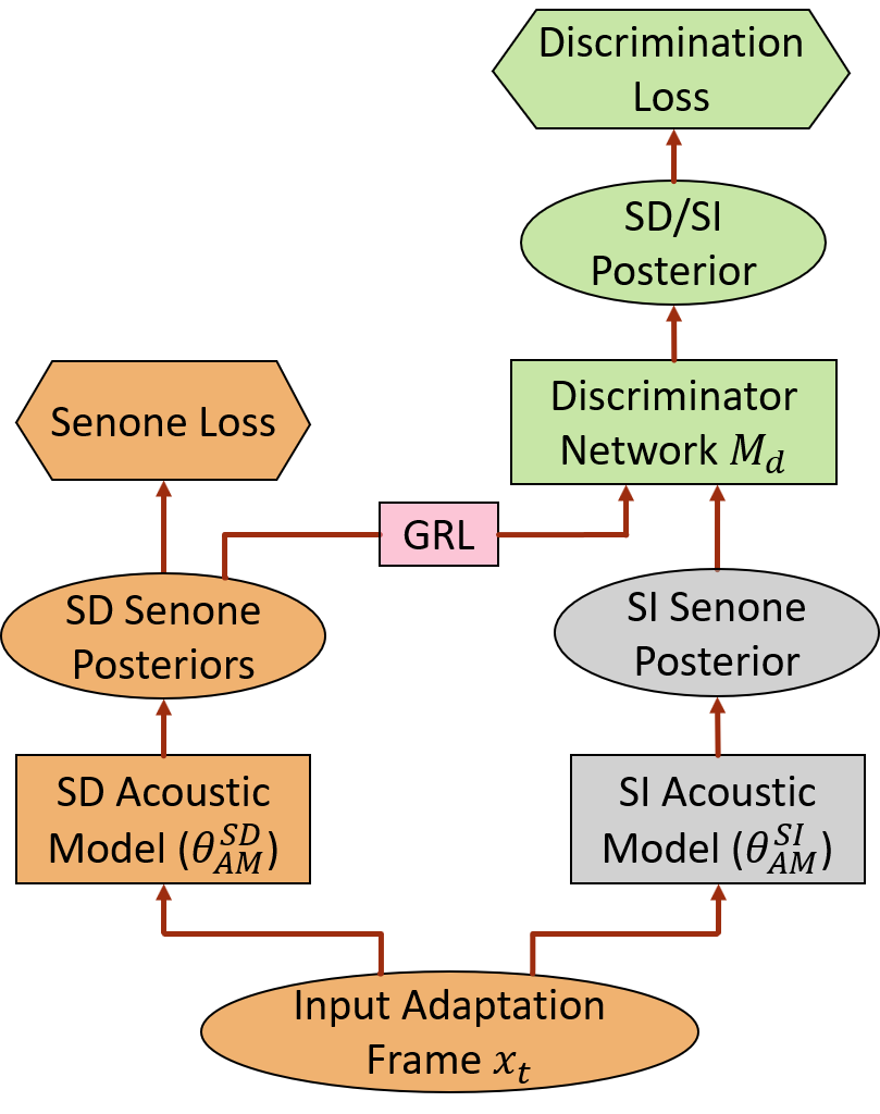
Fig. 2: The framework of ASA-SP. The SI acoustic model is fixed during ASA-SP. Only the SD acoustic model is used in ASR.

In this case, the discriminator $M_{d}$ takes $p(s|\mathbf{x}_{t};\mathbf{\theta}^{\text{SD}}_{\text{AM}})$ and $p(s|\mathbf{x}_{t};\mathbf{\theta}^{\text{SI}}_{\text{AM}})$ as the input and predicts the posterior that the input is generated by the SD model. The discrimination loss $\mathcal{L}_{\text{disc}}(\theta_{f},\theta_{d})$ for $M_{d}$ is formulated below using cross-entropy:

$$\mathcal{L}_{\text{disc}}(\theta^{\text{SD}}_{\text{AM}},\theta_{d})=-\frac{1}{T}\sum_{t=1}^{T}\left[\log p(\mathbf{y}_{t}^{\text{SD}}\in\mathbbm{E}_{\text{SD}}|\mathbf{x}_{t};\theta^{\text{SD}}_{\text{AM}},\theta_{d})\right.$$

$$\qquad\qquad\qquad\qquad\qquad\left.+\log p(\mathbf{y}_{t}^{\text{SI}}\in\mathbbm{E}_{\text{SI}}|\mathbf{x}_{t};\theta^{\text{SI}}_{\text{AM}},\theta_{d})\right],$$ (15)

where $\mathbbm{E}_{\text{SD}}$ and $\mathbbm{E}_{\text{SI}}$ denote the sets of senone posterior vectors generated by SD and SI models, respectively. Similar adversarial MTL is performed to make the distributions of $\mathbf{Y}^{\text{SD}}=\{\mathbf{y}^{\text{SD}}_{1},\ldots,\mathbf{y}^{\text{SD}}_{T}\}$ similar to that of $\mathbf{Y}^{\text{SI}}=\{\mathbf{y}^{\text{SI}}_{1},\ldots,\mathbf{y}^{\text{SI}}_{T}\}$ below:

$$(\hat{\mathbf{\theta}}_{\text{AM}}^{\text{SD}}) =\operatorname*{arg\,min}_{\mathbf{\theta}_{\text{AM}}^{\text{SD}}}\mathcal{L}_{\text{senone}}(\mathbf{\theta}_{\text{AM}}^{\text{SD}})-\lambda\mathcal{L}_{\text{disc}}(\mathbf{\theta}_{\text{AM}}^{\text{SD}},\mathbf{\theta}_{\text{AM}}^{\text{SI}},\hat{\mathbf{\theta}}_{d}),$$ (16)

$$(\hat{\mathbf{\theta}}_{d}) =\operatorname*{arg\,min}_{\mathbf{\theta}_{d}}\mathcal{L}_{\text{disc}}(\hat{\mathbf{\theta}}_{\text{AM}}^{\text{SD}},\mathbf{\theta}_{\text{AM}}^{\text{SI}},\mathbf{\theta}_{d}).$$ (17)

$\mathbf{\theta}_{\text{AM}}^{\text{SI}}$ is optimized by back propagation below, $\mathbf{\theta}_{d}$ is optimized via Eq. (13) and $\mathbf{\theta}_{\text{AM}}^{\text{SI}}$ remain unchanged during the optimization.

$$\mathbf{\theta}_{\text{AM}}^{\text{SD}}\leftarrow\mathbf{\theta}_{\text{AM}}^{\text{SD}}-\mu\left[\frac{\partial\mathcal{L}_{\text{senone}}}{\partial\mathbf{\theta}_{f}^{\text{SD}}}-\lambda\frac{\partial\mathcal{L}_{\text{disc}}}{\partial\mathbf{\theta}_{\text{AM}}^{\text{SD}}}\right].$$ (18)

ASA-SP is an extension of ASA where the deep hidden feature moves up to the output layer and becomes the senone posteriors vector. In this case, the senone classifier disappears and the feature extractor becomes the entire acoustic model.

4 Experiments

We perform speaker adaptation on a Microsoft Windows Phone SMD task. The training data consists of 2600 hours of Microsoft internal live US English data collected through a number of deployed speech services including voice search and SMD. The test set consists of 7 speakers with a total number of 20,203 words. Four adaptation sets of 20, 50, 100 and 200 utterances per speaker are used for acoustic model adaptation, respectively, to explore the impact of adaptation data duration. Any adaptation set with smaller number of utterances is a subset of a larger one.

4.1 Baseline System

We train an SI long short-term memory (LSTM)-hidden Markov model (HMM) acoustic model [34, 35, 36] with 2600 hours of training data. This SI model has 4 hidden layers with 1024 units in each layer and the output size of each hidden layer is reduced to 512 by a linear projection. 80-dimensional log Mel filterbank features are extracted from training, adaptation and test data. The output layer has a dimension of 5980. The LSTM is trained to minimize the frame-level cross-entropy criterion. There is no frame stacking, and the output HMM state label is delayed by 5 frames. A trigram LM is used for decoding with around 8M n-grams. This SI LSTM acoustic model achieves 13.95% WER on the SMD test set.

We further perform KLD speaker adaptation [11] with different regularization weights $\rho$. In Tables 1 and 2, KLD with $\rho=0.5$ achieves 12.54% - 13.24% and 13.55% - 13.85% WERs for supervised and unsupervised adaption, respectively with 20 - 200 adaptation utterances.

System	Number of Adaptation Utterances
	20	50	100	200	Avg.
SI	13.95
KLD ($\rho=0.0$)	13.68	13.39	13.31	13.21	13.40
KLD ($\rho=0.2$)	13.20	13.00	12.71	12.61	12.88
KLD ($\rho=0.5$)	13.24	13.08	12.85	12.54	12.93
KLD ($\rho=0.8$)	13.55	13.50	13.46	13.17	13.42
ASA ($\lambda=1.0$)	12.99	12.86	12.56	12.05	12.62
ASA ($\lambda=3.0$)	13.03	12.72	12.35	11.94	12.56
ASA ($\lambda=5.0$)	13.14	12.71	12.50	12.06	12.60
ASA-SP ($\lambda=1.0$)	13.04	12.88	12.66	12.17	12.69
ASA-SP ($\lambda=3.0$)	13.05	12.89	12.67	12.18	12.70
ASA-SP ($\lambda=5.0$)	13.05	12.89	12.69	12.18	12.70

Table 1: The WER (%) performance of supervised speaker adaptation using KLD and ASA with different $\lambda$ on Microsoft SMD task.

System	Number of Adaptation Utterances
	20	50	100	200	Avg.
SI	13.95
KLD ($\rho=0.0$)	14.18	14.01	13.81	13.73	13.93
KLD ($\rho=0.2$)	13.86	13.83	13.75	13.65	13.77
KLD ($\rho=0.5$)	13.85	13.80	13.73	13.55	13.73
KLD ($\rho=0.8$)	13.89	13.86	13.80	13.72	13.82
ASA ($\lambda=1.0$)	13.74	13.70	13.38	12.99	13.45
ASA ($\lambda=3.0$)	13.66	13.61	13.09	12.85	13.30
ASA ($\lambda=5.0$)	13.85	13.69	13.27	13.03	13.46
ASA-SP ($\lambda=1.0$)	13.83	13.72	13.48	13.16	13.55
ASA-SP ($\lambda=3.0$)	13.84	13.74	13.53	13.17	13.57
ASA-SP ($\lambda=5.0$)	13.85	13.74	13.52	13.16	13.57

Table 2: The WER (%) performance of unsupervised speaker adaptation using KLD and ASA with different $\lambda$ on Microsoft SMD task.

4.2 Adversarial Speaker Adaptation

We perform standard ASA as described in Section 4.2. The SI feature extractor $M_{f}^{\text{SI}}$ is formed as the first $N_{h}$ layers of the SI LSTM and the SI senone classifier $M_{y}^{\text{SI}}$ is the rest $(4-N_{h})$ hidden layers plus the output layer. The SD feature extractor $M_{f}^{\text{SD}}$ and SD senone classifier $M_{y}^{\text{SD}}$ are cloned from $M_{f}^{\text{SI}}$ and $M_{y}^{\text{SI}}$, respectively as an initialization. $N_{h}$ indicates the position of the deep hidden feature in the SD and SI LSTMs. $M_{d}$ is a feedforward DNN with 2 hidden layers and 512 hidden units for each layer. The output layer of $M_{d}$ has 1 unit predicting the posteriors of input deep feature generated by the $M_{f}^{\text{SD}}$. $M_{d}$ has 512-dimensional input layer. $M_{f}^{\text{SD}}$, $M_{y}^{\text{SD}}$ and $M_{d}$ are jointly trained with an adversarial MTL objective. Due to space limitation, we only show the results when $N_{h}=4$.

For supervised ASA, the same alignment is used as in KLD. In Table 1, the best ASA setups achieve 12.99%, 12.71%, 12.35% and 11.94% WERs for 20, 50, 100, 200 adaptation utterances which improve the WERs by 6.9%, 8.9%, 11.5%, 14.4% relatively over the SI LSTM, respectively. Supervised ASA ($\lambda=3.0$) also achieves up to 5.3% relative WER reduction over the best KLD setup ($\rho=0.2$).

For unsupervised ASA, the same decoded senone labels are used as in KLD. In Table 2, the best ASA setups achieve 13.66%, 13.61%, 13.09% and 12.85% WERs for 20, 50, 100, 200 adaptation utterances which improves the WERs by 2.1%, 2.4%, 6.2%, 7.9% relatively over the SI LSTM, respectively. Unsupervised ASA ($\lambda=3.0$) also achieves up to and 5.2% relatively WER gains over the best KLD setup ($\rho=0.5$). Compared with supervised ASA, the unsupervised one decreases the relative WER gain over the SI LSTM by about half on the same number of adaptation utterances.

For both supervised and unsupervised ASA, the WER first decreases as $\lambda$ grows larger and then increases when $\lambda$ becomes too large. ASA performs consistently better than SI LSTM and KLD with different number of adaptation utterances for both supervised and unsupervised adaptation. The relative gain increases as the number of adaptation utterance grows.

4.3 Adversarial Speaker Adaptation on Senone Posteriors

We then perform ASA-SP as described in Section 4.2. The SD acoustic model is cloned from the SI LSTM as the initialization. $M_{d}$ shares the same architecture as the one in Section 4.2. In Table 1, for supervised adaptation ASA-SP $(\lambda=1.0)$ achieves 6.5%, 7.7%, 9.2%, 12.8% relative WER gain over the SI LSTM, respectively and up to 3.5% relative WER reduction over the best KLD setup ($\rho=0.2$). In Table 2, for unsupervised adaptation ASA-SP $(\lambda=1.0)$ achieves 0.9%, 1.6%, 3.4%, 5.7%, 2.9% relative WER gain over the SI LSTM, respectively and up to 4.8% relative WER reduction over the best KLD setup ($\rho=0.5$).

Although ASA-SP consistently improves over KLD on different number of adaptation utterances for both supervised and unsupervised adaptation, it performs worse than standard ASA where the regularization from SI model is performed at the hidden layers. The reason is that the senone posteriors vectors $\mathbf{y}^{\text{SI}}_{t}$, $\mathbf{y}^{\text{SD}}_{t}$ lie in a much higher-dimensional space than the deep features $\mathbf{f}^{\text{SI}}_{t}$, $\mathbf{f}^{\text{SD}}_{t}$ so that the discriminator is much harder to learn given much sparser-distributed samples. We also notice that ASA-SP performance is much less sensitive to the variation of $\lambda$ compared with standard ASA.

5 Conclusion

In this work, a novel adversarial speaker adaptation method is proposed, in which the deep hidden features (ASA) or the output senone posteriors (ASA-SP) of an SD DNN acoustic model are forced by the adversarial MTL to conform to a similar distribution as those of a fixed reference SI DNN acoustic model while being trained to be senone-discriminative with the limited adaptation data.

We evaluate ASA on Microsoft SMD task with 2600 hours of training data. ASA achieves up to 14.4% and 7.9% relative WER gain for supervised and unsupervised adaptation, respectively, over the SI LSTM acoustic model. ASA also improves consistently over the KLD regularization method. The relative gain grows as the number of adaption utterances increases. ASA-SP performs consistently better than KLD but worse than the standard ASA.

References

- [1] G. Hinton, L. Deng, D. Yu, et al., “Deep neural networks for acoustic modeling in speech recognition: The shared views of four research groups,” IEEE Signal Processing Magazine, vol. 29, no. 6, pp. 82–97, 2012.
- [2] Dong Yu and Jinyu Li, “Recent progresses in deep learning based acoustic models,” IEEE/CAA Journal of Automatica Sinica, vol. 4, no. 3, pp. 396–409, 2017.
- [3] J. Li, L. Deng, Y. Gong, and R. Haeb-Umbach, “An overview of noise-robust automatic speech recognition,” IEEE/ACM Transactions on Audio, Speech and Language Processing, vol. 22, no. 4, pp. 745–777, April 2014.
- [4] J. Neto, L. Almeida, M. Hochberg, et al., “Speaker-adaptation for hybrid hmm-ann continuous speech recognition system,” in Proc. Eurospeech, 1995.
- [5] R. Gemello, F. Mana, S. Scanzio, et al., “Linear hidden transformations for adaptation of hybrid ann/hmm models,” Speech Communication, vol. 49, no. 10, pp. 827 – 835, 2007.
- [6] Jian Xue, Jinyu Li, and Yifan Gong, “Restructuring of deep neural network acoustic models with singular value decomposition.,” in Interspeech, 2013, pp. 2365–2369.
- [7] Y. Zhao, J. Li, and Y. Gong, “Low-rank plus diagonal adaptation for deep neural networks,” in Proc. ICASSP, March 2016, pp. 5005–5009.
- [8] G. Saon, H. Soltau, D. Nahamoo, and M. Picheny, “Speaker adaptation of neural network acoustic models using i-vectors,” in Proc. ASRU, Dec 2013, pp. 55–59.
- [9] O. Abdel-Hamid and H. Jiang, “Fast speaker adaptation of hybrid nn/hmm model for speech recognition based on discriminative learning of speaker code,” in Proc. ICASSP, May 2013, pp. 7942–7946.
- [10] S. Xue, O. Abdel-Hamid, H. Jiang, L. Dai, and Q. Liu, “Fast adaptation of deep neural network based on discriminant codes for speech recognition,” in TASLP, vol. 22, no. 12, pp. 1713–1725, Dec 2014.
- [11] D. Yu, K. Yao, H. Su, G. Li, and F. Seide, “Kl-divergence regularized deep neural network adaptation for improved large vocabulary speech recognition,” in Proc. ICASSP, May 2013, pp. 7893–7897.
- [12] Zhong Meng, Jinyu Li, Yong Zhao, and Yifan Gong, “Conditional teacher-student learning,” in Proc. ICASSP, 2019.
- [13] Z. Huang, S. Siniscalchi, I. Chen, et al., “Maximum a posteriori adaptation of network parameters in deep models,” in Proc. Interspeech, 2015.
- [14] Z. Huang, J. L, S. Siniscalchi., et al., “Rapid adaptation for deep neural networks through multi-task learning.,” in Interspeech, 2015, pp. 3625–3629.
- [15] I. Goodfellow, J. Pouget-Adadie, et al., “Generative adversarial nets,” in Proc. NIPS, pp. 2672–2680. 2014.
- [16] S. Sun, B. Zhang, L. Xie, et al., “An unsupervised deep domain adaptation approach for robust speech recognition,” Neurocomputing, vol. 257, pp. 79 – 87, 2017.
- [17] Z. Meng, Z. Chen, V. Mazalov, J. Li, and Y. Gong, “Unsupervised adaptation with domain separation networks for robust speech recognition,” in Proc. ASRU, 2017.
- [18] Yusuke Shinohara, “Adversarial multi-task learning of deep neural networks for robust speech recognition.,” in INTERSPEECH, 2016, pp. 2369–2372.
- [19] D. Serdyuk, K. Audhkhasi, P. Brakel, B. Ramabhadran, et al., “Invariant representations for noisy speech recognition,” in NIPS Workshop, 2016.
- [20] Zhong Meng, Jinyu Li, Yifan Gong, and Biing-Hwang Juang, “Adversarial teacher-student learning for unsupervised domain adaptation,” in Proc. ICASSP. IEEE, 2018, pp. 5949–5953.
- [21] Z. Meng, J. Li, Z. Chen, et al., “Speaker-invariant training via adversarial learning,” in Proc. ICASSP, 2018.
- [22] G. Saon, G. Kurata, T. Sercu, et al., “English conversational telephone speech recognition by humans and machines,” arXiv preprint arXiv:1703.02136, 2017.
- [23] Zhong Meng, Jinyu Li, and Yifan Gong, “Attentive adversarial learning for domain-invariant training,” in Proc. ICASSP, 2019.
- [24] Santiago Pascual, Antonio Bonafonte, and Joan Serrà, “Segan: Speech enhancement generative adversarial network,” in Interspeech, 2017.
- [25] Zhong Meng, Jinyu Li, and Yifan Gong, “Adversarial feature-mapping for speech enhancement,” Interspeech, 2018.
- [26] Zhong Meng, Jinyu Li, and Yifan Gong, “Cycle-consistent speech enhancement,” Interspeech, 2018.
- [27] Q. Wang, W. Rao, S. Sun, L. Xie, E. S. Chng, and H. Li, “Unsupervised domain adaptation via domain adversarial training for speaker recognition,” ICASSP 2018, 2018.
- [28] Zhong Meng, Yong Zhao, Jinyu Li, and Yifan Gong, “Adversarial speaker verification,” in Proc. ICASSP, 2019.
- [29] Yaroslav Ganin and Victor Lempitsky, “Unsupervised domain adaptation by backpropagation,” in Proc. ICML, Lille, France, 2015, vol. 37, pp. 1180–1189, PMLR.
- [30] K. Bousmalis, G. Trigeorgis, N. Silberman, et al., “Domain separation networks,” in Proc. NIPS, D. D. Lee, M. Sugiyama, U. V. Luxburg, I. Guyon, and R. Garnett, Eds., pp. 343–351. Curran Associates, Inc., 2016.
- [31] Solomon Kullback and Richard A Leibler, “On information and sufficiency,” The annals of mathematical statistics, vol. 22, no. 1, pp. 79–86, 1951.
- [32] Will Kurt, “Kullback-leibler divergence explained,” https://www.countbayesie.com/blog/2017/5/9/kullback-leibler-divergence-explained, 2017.
- [33] Ben Moran, “Kullback-leibler divergence asymmetry,” https://benmoran.wordpress.com/2012/07/14/kullback-leibler-divergence-asymmetry/, 2012.
- [34] F. Beaufays H. Sak, A. Senior, “Long short-term memory recurrent neural network architectures for large scale acoustic modeling,” in Interspeech, 2014.
- [35] Z. Meng, S. Watanabe, J. R. Hershey, et al., “Deep long short-term memory adaptive beamforming networks for multichannel robust speech recognition,” in ICASSP. IEEE, 2017, pp. 271–275.
- [36] H. Erdogan, T. Hayashi, J. R. Hershey, et al., “Multi-channel speech recognition: Lstms all the way through,” in CHiME-4 workshop, 2016, pp. 1–4.