$Sp(4;\mathbb{R})$ Squeezing for Bloch Four-Hyperboloid
via
The Non-Compact Hopf Map

Kazuki Hasebe

National Institute of Technology, Sendai College, Ayashi, Sendai, 989-3128, Japan

khasebe@sendai-nct.ac.jp

We explore the hyperbolic geometry of squeezed states in the perspective of the non-compact Hopf map. Based on analogies between squeeze operation and $Sp(2,\mathbb{R})$ hyperbolic rotation, two types of the squeeze operators, the (usual) Dirac- and the Schwinger-types, are introduced. We clarify the underlying hyperbolic geometry and $SO(2,1)$ representations of the squeezed states along the line of the 1st non-compact Hopf map. Following to the geometric hierarchy of the non-compact Hopf maps, we extend the $Sp(2;\mathbb{R})$ analysis to $Sp(4;\mathbb{R})$ — the isometry of an split-signature four-hyperboloid. We explicitly construct the $Sp(4;\mathbb{R})$ squeeze operators in the Dirac- and Schwinger-types and investigate the physical meaning of the four-hyperboloid coordinates in the context of the Schwinger-type squeezed states. It is shown that the Schwinger-type $Sp(4;\mathbb{R})$ squeezed one-photon state is equal to an entangled superposition state of two $Sp(2;\mathbb{R})$ squeezed states and the corresponding concurrence has a clear geometric meaning. Taking advantage of the group theoretical formulation, basic properties of the $Sp(4;\mathbb{R})$ squeezed coherent states are also investigated. In particular, we show that the $Sp(4;\mathbb{R})$ squeezed vacuum naturally realizes a generalized squeezing in a 4D manner.

1 Introduction

Qubit is a most fundamental object in the study of quantum information and quantum optics. Polarization of the qubit is specified by a point of the Bloch sphere [1], and, in the Lie group language of Perelomov [2], the qubit is the $SU(2)$ spin coherent state (of spin magnitude $1/2$) [3]. It is well known that the geometry of the Bloch sphere is closely related to the Hopf map [4]: Qubit is a two-component normalized spinor geometrically representing $S^{3}$ and its overall $U(1)$ phase is not relevant to physics, so the physical space of the qubit is given by the projected space of the 1st Hopf map, $S^{3}/U(1)\simeq S^{3}/S^{1}\simeq S^{2}$. It is also reported that the 2nd and 3rd Hopf maps that represent topological maps from spheres to spheres in different dimensions [5] are sensitive to the entanglement of qubits [7, 8, 9]. Spherical geometries thus play important roles in describing the geometry of quantum states. Beyond spheres, one can find many applications of $\it{compact}$ manifolds in the geometry of quantum states [10]. Meanwhile, hyperboloids or more generally $\it{non}$-$\it{compact}$ manifolds have been elusive in applications to the study of geometry of quantum states, although a hyperbolic nature inherent to quantum mechanics is glimpsed in the Bogoliubov canonical transformation that keeps the bosonic canonical commutation relations. For $n$ species of bosonic operators, the Bogoliubov transformation is described by the symplectic group $Sp(2n;\mathbb{R})$ [13, 14, 15]. The simplest symplectic group is $Sp(2;\mathbb{R})\simeq SU(1,1)$, which is the double cover of the $SO(2,1)$ isometry group of two-hyperboloid. Since $SU(1,1)$ is a non-compact counterpart of $SU(2)$, one can mathematically develop an argument similar to $SU(2)$: The $SU(1,1)$ hyperbolic “rotation” gives rise to the pseudo-spin coherent state [2, 15, 16, 17, 18], and the $SU(1,1)$ pseudo-spin coherent state is specified by a position on the Bloch two-hyperboloid, $H^{2,0}$. What is interesting is that the hyperbolic rotation is not a purely mathematical concept but closely related to quantum optics as squeeze operation [19, 20, 21]. The squeeze operator or squeezed state has more than forty year history, since its theoretical proposal in quantum optics [22, 23, 24, 25, 26, 27]. There are a number of literatures about the squeezed state. For instance, $n$-mode generalization of the squeezed state was investigated in Refs. [28, 19, 29, 30, 31, 32, 33, 34, 35], and also fermionic and supersymmetric squeezed states in [36, 37, 38, 39, 40, 41]. Interested readers may consult Ref.[42] as a nice review of the history of squeezed states and references therein. Here, we may encapsulate the above observation as

Qubit state $$\rightarrow~{}~{}~{}~{}~{}~{}~{}~{}~{}\text{Point on the Bloch sphere}~{}~{}~{}~{}~{}~{}~{}~{}~{}\rightarrow~{}~{}SU(2)~{}\text{spin coherent state},$$

$$~{}~{}~{}~{}~{}~{}~{}~{}~{}~{}~{}~{}~{}~{}~{}~{}~{}~{}~{}~{}~{}~{}~{}~{}~{}~{}~{}~{}~{}~{}~{}~{}~{}~{}~{}~{}~{}~{}~{}~{}~{}~{}~{}~{}~{}~{}~{}~{}~{}~{}~{}~{}~{}~{}~{}~{}~{}~{}~{}~{}~{}~{}~{}~{}~{}~{}~{}~{}~{}~{}~{}~{}~{}~{}~{}~{}~{}~{}~{}~{}\downarrow$$

Squeezed state $$\leftarrow~{}~{}~{}~{}~{}~{}\text{Point on the Bloch hyperboloid}~{}~{}~{}~{}~{}\leftarrow~{}~{}SU(1,1)~{}\text{pseudo-spin coherent state}.$$

Interestingly, the hyperbolic Berry phase associated with the squeezed state was pointed out in [43, 44], and subsequently the hyperbolic Berry phase was observed in experiments [45]. The geometry behind the hyperbolic Berry phase is the 1st non-compact Hopf map, $H^{2,1}/U(1)\simeq H^{2,0}$.

About a decade ago, the author proposed a non-compact version of the Hopf maps based on the split algebras [46, 47]:

		$H^{2,1}$	$\overset{H^{0,1}=S^{1}}{\longrightarrow}$	$H^{2,0}$		(1st)
	$H^{4,3}$	$\longrightarrow$	$H^{2,2}$			(2nd)
$H^{8,7}$	$\longrightarrow$	$H^{4,4}$				(3rd)

Just as in the original Hopf maps, the non-compact Hopf maps exhibit a dimensional hierarchy in a hyperbolic manner. Taking advantage of such hierarchical structure, we extend the formulation of the squeezed states previously restricted to the $Sp(2;\mathbb{R})$ group to the $Sp(4;\mathbb{R})$ group based on the 2nd non-compact Hopf map. The base-manifold of the 2nd Hopf map is a split-signature four-hyperboloid, $H^{2,2}$, with isometry group $SO(2,3)$ whose double cover is $Spin(2,3)~{}\simeq~{}Sp(4;\mathbb{R})$ — the next-simplest symplectic group of the Bogoliubov transformation for two bosonic operators [48, 49]. The main goal of the present work is to construct the $Sp(4;\mathbb{R})$ squeezed state explicitly and clarify its basic properties. To begin with, we rewrite the single-mode and two-mode operators of $Sp(2;\mathbb{R})$ in a perspective of the $SO(2,1)$ group representation theory. We then observe the following correspondences:

$Sp(2;\mathbb{R})$ one-/two-mode squeezing   $\longleftrightarrow$  $SO(2,1)~{}\text{Majorana/Dirac~{}representation}$.
For two-mode squeezing, the $Sp(4;\mathbb{R})$ background symmetry has been suggested in Refs.[28, 19, 29, 30, 31, 32, 33, 34]. We will discuss that the $Sp(4;\mathbb{R})$ symmetry is naturally realized in the context of the Majorana representation of $SO(2,3)$. In a similar manner to the $Sp(2;\mathbb{R})$ case, we introduce a four-mode squeeze operator as Dirac representation of $SO(2;3)$,

$Sp(4;\mathbb{R})$ two-/four-mode squeezing   $\longleftrightarrow$  $SO(2,3)~{}\text{Majorana/Dirac~{}representation}$,
and investigate their particular properties. We introduce two types of squeeze operator, the (usual) Dirac- and Schwinger-type. In the case of $Sp(2;\mathbb{R})$ squeezing, the Dirac- and the Schwinger-type squeeze operators generate physically equivalent squeezed vacua, while in the case of $Sp(4;\mathbb{R})$, two types of squeezing generate physically distinct squeezed vacua.

It may be worthwhile to mention peculiar properties of hyperboloids not observed in spheres. We can simply switch from spherical geometry to hyperbolic geometry by flipping several signatures of metric, but hyperboloids have unique properties intrinsic to their non-compactness. First, the non-compact isometry groups, such as $SO(2,1)$ and $SO(2,3)$, accommodate Majorana representation, while their compact counterparts, $SO(3)$ and $SO(5)$, do not. Second, unitary representations of non-compact groups are infinite dimensional and very distinct from finite unitary representations of compact groups. Third, non-compact groups exhibit more involved topological structures than those of their compact counterparts. For instance, the compact $USp(2)\simeq Spin(3)\simeq S^{3}$ is simply connected, while $Sp(2;\mathbb{R})\simeq Spin(2,1)\simeq H^{2,1}\simeq R^{2}\otimes S^{1}$ is not and leads to the projective representation called the metaplectic representation [50, 51]. A similar relation holds for $Sp(4;\mathbb{R})\simeq Spin(2,3)$ and $USp(4)\simeq Spin(5)$.

This paper is organized as follows. Sec.2 presents Hermitian realization of non-compact algebra with pseudo-Hermiticity. The topology of symplectic groups is also reviewed. We discuss the $Sp(2;\mathbb{R})$ squeezing in the context of the 1st non-compact Hopf map and identify $Sp(2;\mathbb{R})$ one- and two-mode operators with the $SO(2,1)$ Majorana and Dirac representations in Sec.3. Sec.4 gives the Majorana and Dirac representations of the $SO(2,3)$ group and the factorization of the $Sp(4;\mathbb{R})$ non-unitary coset matrix with emphasis on its relation to the non-compact 2nd Hopf map. In Sec.5, we explicitly construct the $Sp(4;\mathbb{R})$ squeezed states and investigate their properties. We also extend the analysis to the $Sp(4;\mathbb{R})$ squeezed coherent states in Sec.6. Sec.7 is devoted to summary and discussions.

2 Pseudo-Hermitian matrices and symplectic group

We develop a Schwinger boson construction of unitary operators for non-compact groups with pseudo-Hermiticity. Topological structures of the symplectic groups and ultra-hyperboloids are also briefly reviewed.

2.1 Hermitian operators made of the Schwinger bosons

While unitary representations of non-compact groups are not finite dimensional, non-unitary representations are finite dimensional. Suppose that $t^{a}$ are non-Hermitian matrices that satisfy the algebra

$$[t^{a},t^{b}]=if^{abc}t_{c},$$ (1)

where $f^{abc}$ denote the structure constants of the non-compact algebra. In the following, we assume that there exists a matrix $k$ that makes $kt^{a}$ be hermitian,

$$(kt^{a})^{\dagger}=kt^{a}$$ (2)

or

$$(t^{a})^{\dagger}=k~{}t^{a}~{}(k^{\dagger})^{-1}.$$ (3)

Needless to say, it is not generally guaranteed about the existence of such a matrix $k$. If there exists $k$ satisfying (2), the matrices $t^{a}$ are referred to as the pseudo-Hermitian matrices [52, 53]. With the pseudo-Hermitian matrices, it is straightforward to construct Hermitian operators sandwiching the pseudo-Hermitian matrices by the Schwinger boson operator $\hat{\phi}_{\alpha}$ and its conjugate:

$$X^{a}=\hat{\phi}_{\alpha}^{\dagger}~{}(kt^{a})_{\alpha\beta}~{}\hat{\phi}_{\beta}=\hat{\phi}^{\dagger}~{}kt^{a}\hat{\phi}=\bar{\hat{\phi}}~{}t^{a}\hat{\phi},$$ (4)

where

$$\bar{\hat{\phi}}\equiv\hat{\phi}^{\dagger}k.$$ (5)

We determine the commutation relations of the components $\hat{\phi}_{\alpha}$ so that $X^{a}$ satisfy the same algebra as (1):

$$[X^{a},X^{b}]=if^{abc}X_{c}.$$ (6)

The commutation relations among $\hat{\phi}_{\alpha}$ are thus determined as

$$[\hat{\phi}_{\alpha},\bar{\hat{\phi}}_{\beta}]=\delta_{\alpha\beta},$$ (7)

or

$$[\hat{\phi}_{\alpha},\hat{\phi}^{\dagger}_{\beta}]=(k^{-1})_{\alpha\beta}.$$ (8)

Notice that while $t^{a}$ are non-Hermitian matrices, $X^{a}$ are Hermitian operators. With generators $X^{a}$, it is straightforward to construct elements of non-compact group:

$$S=e^{-i\omega_{a}X^{a}},$$ (9)

with $\omega_{a}$ being group parameters. Obviously, $S$ is a unitary operator

$$S^{\dagger}=S^{-1}.$$ (10)

From the non-Hermitian matrix $t^{a}$, we can construct the non-unitary matrix element of the non-compact group as

$$M=e^{-i\omega_{a}t^{a}},$$ (11)

which satisfies the pseudo-unitary condition:

$$M^{\dagger}=kM^{-1}(k^{\dagger})^{-1}.$$ (12)

$X^{a}$ act to $\hat{\phi}$ as

$$[X^{a},\hat{\phi}_{\alpha}]=-(t^{a})_{\alpha\beta}\hat{\phi}_{\beta}$$ (13)

or

$$[X^{a},\bar{\phi}_{\alpha}]=\bar{\phi}_{\beta}(t^{a})_{\beta\alpha},$$ (14)

which means that $\hat{\phi}$ behaves as the spinor representation of the non-compact group generated by $X^{a}$. We then have

$$S^{\dagger}~{}\hat{\phi}~{}S=M\hat{\phi},$$ (15)

and

$$S~{}\bar{\hat{\phi}}~{}S^{\dagger}=\bar{\hat{\phi}}~{}M^{-1},$$ (16)

where

$$M^{-1}=e^{i\omega_{a}t^{a}}=k^{-1}M^{\dagger}k^{\dagger}.$$ (17)

Notice that while $S$ is a $\it{unitary}$ operator, $M$ is a $\it{non}$-$\it{unitary}$ matrix. Both of them are specified by the same parameters $\omega_{a}$, and so there exists one-to-one mapping between them. When $S$ acts to a normalized state $|n\rangle$ $(\langle n|n\rangle=1)$, the magnitude does not change under the transformation of the non-compact group as shown by $\langle n|S^{\dagger}S|n\rangle=1$. In the matrix notation, however, the transformation does not preserve the magnitude of a normalized vector $\boldsymbol{n}$ ($\boldsymbol{n}^{\dagger}\boldsymbol{n}=1$) as implied by $\boldsymbol{n}^{\dagger}M^{\dagger}M\boldsymbol{n}\neq\boldsymbol{n}^{\dagger}\boldsymbol{n}$. This does not occur in usual discussions of quantum mechanics for compact Lie groups, since we can realize the group elements by a finite dimensional unitary matrix. In non-compact Lie groups, finite dimensional unitary representation does not exist, however, when we adopt the unitary operator $S$ made by the Hermitian operators $X_{a}$, the probability conservation still holds, and so we do not need to worry about going beyond the usual probability interpretation of quantum mechanics.

In this paper, we mainly utilize the real symplectic groups $Sp(2n;\mathbb{R})=U(n;\mathbb{H}^{\prime})$, and we here summarize the basic properties of $Sp(2n;\mathbb{R})$ [see Appendix A also]. The generators of $Sp(2n;\mathbb{R})$ are represented by a $2n\times 2n$ matrix of the following form (310):

$$X=\begin{pmatrix}H&S^{*}\\ -S&-H^{*}\end{pmatrix},$$ (18)

where $H$ is a $n\times n$ Hermitian matrix and $S$ a $n\times n$ symmetric complex matrix. Though $X$ itself is non-Hermitian in general, there obviously exists a matrix

$$K=\begin{pmatrix}1_{n}&0\\ 0&-1_{n}\end{pmatrix},$$ (19)

which makes $X$ be Hermitian:

$$KX=\begin{pmatrix}H&S^{*}\\ S&H^{*}\end{pmatrix}.$$ (20)

In this sense, the $sp(2n;\mathbb{R})$ matrix generators are pseudo-Hermitian, and we can construct the Hermitian $sp(2n;\mathbb{R})$ operators by following the general method discussed above.

2.2 Topology of the symplectic groups and ultra-hyperboloids

Here, we review geometric properties of the symplectic groups. The polar decomposition of $Sp(2n;\mathbb{R})$ group is given by[54]

$$Sp(2n;\mathbb{R})~{}\simeq~{}U(n)\otimes\mathbb{R}^{n(n+1)}~{}\simeq~{}U(1)\otimes SU(n)\otimes\mathbb{R}^{n(n+1)},$$ (21)

where $U(n)$ is the maximal Cartan subgroup of $Sp(2n;\mathbb{R})$. In particular, we have

$$Sp(2;\mathbb{R})\simeq U(1)\otimes\mathbb{R}^{2}\simeq S^{1}\otimes\mathbb{R}^{2},$$ (22a)

$$Sp(4;\mathbb{R})\simeq U(1)\otimes SU(2)\otimes\mathbb{R}^{6}\simeq S^{1}\otimes S^{3}\otimes\mathbb{R}^{6}.$$ (22b)

The decomposition (21) implies that the symplectic group is not simply connected:

$$\pi_{1}(Sp(2n;\mathbb{R}))\simeq\pi_{1}(U(1))\simeq\mathbb{Z}.$$ (23)

The double covering of the symplectic group is called the metaplectic group $Mp(2n;\mathbb{R})$:

$$Mp(2n;\mathbb{R})/\mathbb{Z}_{2}\simeq Sp(2n;\mathbb{R}),$$ (24)

and its representation is referred to as the metaplectic representation which is the projective representation of the symplectic group. Note that projective representation does not exist in the compact group counterparts of $Sp(2n;\mathbb{R})$, $i.e.$, $USp(2n)$.

The coset spaces between the symplectic groups are given by

$$Sp(2n+2;\mathbb{H}^{\prime})/Sp(2n;\mathbb{H}^{\prime})~{}\simeq~{}H^{2n+2,2n+1},$$ (25)

where $H^{p,q}$ is referred to as the ultra-hyperboloid $H^{p,q}$ that is a $(p+d)$ dimensional manifold embedded in $\mathbb{R}^{p,q+1}$ as

$$\sum_{i=1}^{p}{x^{i}}{x^{i}}-\sum_{j=1}^{q+1}x^{p+j}x^{p+j}=-1.$$ (27)

(27) implies that as long as $x^{p+j}$ $(j=1,\cdots,q+1)$ is subject to the condition of $q$-dimensional sphere with radius $\sqrt{1+\sum_{i=1}^{p}{x^{i}}{x^{i}}}$, the remaining $p$ real coordinates $x^{i}$ $(i=1,\cdots,p)$ can take any real numbers. Therefore, the topology of $H^{p,q}$ is identified with a fibre-bundle made of base-manifold $\mathbb{R}^{p}$ with fibre $S^{q}$ :

$$H^{p,q}\simeq~{}\mathbb{R}^{p}\otimes S^{q}.$$ (28)

In low dimensions, (28) yields

$$H^{2,0}\simeq\mathbb{R}^{2}\simeq\mathbb{R}_{+}\otimes S^{1},~{}~{}~{}~{}H^{1,1}\simeq\mathbb{R}\otimes S^{1},~{}~{}~{}~{}H^{0,2}\simeq S^{2},$$ (29a)

$$H^{4,0}\simeq\mathbb{R}^{4},~{}H^{3,1}\simeq\mathbb{R}^{3}\otimes S^{1},~{}~{}~{}H^{2,2}\simeq\mathbb{R}^{2}\otimes S^{2},~{}~{}~{}H^{1,3}\simeq\mathbb{R}^{1}\otimes S^{3},~{}~{}~{}H^{0,4}\simeq S^{4}.$$ (29b)

(27) also implies that $H^{p,q}$ can be given by a coset between indefinite orthogonal groups:

$$H^{p,q}~{}\simeq~{}SO(p,q+1)/SO(p,q).$$ (30)

3 $Sp(2;\mathbb{R})$ group and squeezing

The isomorphism $Sp(2;\mathbb{R})~{}\simeq~{}Spin(2,1)$ suggests that the $Sp(2;\mathbb{R})$ one- and two-mode operators are equivalent to the Majorana and the Dirac spinor operators of $SO(2,1)$. Based on the identification of the squeeze operator with the $SU(1,1)\simeq Spin(2,1)$ “rotation” operator, we introduce two types of squeeze operators, the (usual) Dirac- and Schwinger-types. We discuss how the non-compact 1st Hopf map is embedded in the geometry of the $Sp(2;\mathbb{R})$ squeezed state.

3.1 $sp(2;\mathbb{R})$ algebra

From the result of Sec.2.2, we have

$$Mp(2;\mathbb{R})/\mathbb{Z}_{2}~{}\simeq~{}Sp(2;\mathbb{R})~{}\simeq~{}SU(1,1)~{}~{}\simeq~{}Spin(2,1)~{}\simeq~{}H^{2,1}~{}\simeq~{}\mathbb{R}^{2}\times S^{1},$$ (33)

and use the terminologies, $SU(1,1)$ and $Sp(2;\mathbb{R})$, interchangeably. The $su(1,1)$ algebra is defined as

$$[T^{i},T^{j}]=-i\epsilon^{ijk}T_{k}~{}~{}~{}~{}(i,j,k=1,2,3)$$ (34)

with

$$g_{ij}=g^{ij}\equiv\text{diag}(-1,-1,+1),~{}~{}~{}\epsilon^{123}\equiv 1.$$ (35)

We adopt the finite dimensional matrix representation of the $su(1,1)$ generators :

$$\{\frac{1}{2}\tau^{1},\frac{1}{2}\tau^{2},\frac{1}{2}\tau^{3}\}=\{i\frac{1}{2}\sigma_{x},i\frac{1}{2}\sigma_{y},\frac{1}{2}\sigma_{z}\},$$ (36)

which satisfy

$$[\tau^{i},\tau^{j}]=-2i\epsilon^{ijk}\tau_{k},~{}~{}~{}~{}\{\tau^{i},\tau^{j}\}=-2g^{ij}.$$ (37)

Note that $\tau^{1}$ and $\tau^{2}$ are chosen to be non-Hermitian. The completeness relation is given by

$$(\tau^{i})_{\alpha\beta}(\tau_{i})_{\gamma\delta}=2\delta_{\alpha\delta}\delta_{\beta\gamma}-\delta_{\alpha\beta}\delta_{\gamma\delta}.$$ (38)

For later convenience, we introduce the split-quaternions $q^{m}$ $(m=1,2,3,4)$ that are related to the $su(1,1)$ matrices as

$$q^{m}=\{q^{i},1\}=\{-i\tau^{i},1\}=\{\sigma_{x},\sigma_{y},-i\sigma_{z},1\},$$ (39)

and its quaternionic conjugate

$$\bar{q}^{m}=\{-q^{i},1\}=\{i\tau^{i},1\}.$$ (40)

The $Sp(2;\mathbb{R})$ is isomorphic to the split-quaternionic unitary group $U(1;\mathbb{H}^{\prime})$, and in general the real symplectic group is isomorphic to the split-quaternionic unitary group, $Sp(2n;\mathbb{R})\simeq U(n;\mathbb{H}^{\prime})$ (see Appendix A.1).

As mentioned in Sec.2.1, the $sp(2;\mathbb{R})\simeq su(1,1)$ finite dimensional matrix generators (36) are pseudo-Hermitian matrices: With

$$\kappa=\sigma_{z},$$ (41)

we can construct the corresponding Hermitian matrices as

$$\kappa^{i}\equiv\kappa\tau^{i}=\{-\sigma_{y},\sigma_{x},1\}.$$ (42)

$\kappa^{i}$ have the following properties

$$\kappa^{[i}\sigma_{z}\kappa^{j]}=-2i\epsilon^{ijk}\kappa_{k},~{}~{}~{}(\kappa^{i})_{\alpha\beta}(\kappa_{i})_{\gamma\delta}=2(\sigma_{z})_{\alpha\delta}(\sigma_{z})_{\beta\gamma}-(\sigma_{z})_{\alpha\beta}(\sigma_{z})_{\gamma\delta}$$ (43)

where $\kappa^{[i}\sigma_{z}\kappa^{j]}\equiv\kappa^{i}\sigma_{z}\kappa^{j}-\kappa^{j}\sigma_{z}\kappa^{i}$. Since $\kappa^{i}$ are Hermitian, one may immediately see that $g=e^{i\omega_{i}\frac{1}{2}\tau^{i}}$ satisfies

$$g^{\dagger}~{}\sigma_{z}~{}g=\sigma_{z},$$ (44)

which is one of the relations that the $SU(1,1)$ group elements should satisfy. Following the general prescription in Sec.2, we construct the $su(1,1)$ Hermitian operators. We introduce the two-component Schwinger boson operator subject to the condition

$$[\hat{\phi}_{\alpha},\hat{\phi}_{\beta}]=(\sigma_{z})_{\alpha\beta}.$$ (45)

(45) is readily satisfied when we choose

$$\hat{\phi}=\begin{pmatrix}\hat{\phi}_{1}\\ \hat{\phi}_{2}\end{pmatrix}=\begin{pmatrix}a\\ b^{\dagger}\end{pmatrix},$$ (46)

with $a$ and $b$ being two independent Schwinger operators:

$$[a,a^{\dagger}]=[b,b^{\dagger}]=1,~{}~{}~{}~{}[a,b]=[a,b^{\dagger}]=0.$$ (47)

The Hermitian $su(1,1)$ operators are then constructed as

$$T^{i}=\frac{1}{2}~{}\hat{\phi}^{\dagger}~{}\kappa^{i}~{}\hat{\phi},$$ (48)

or

$$T^{x}=i\frac{1}{2}(-ab+a^{\dagger}b^{\dagger}),~{}~{}T^{y}=\frac{1}{2}(ab+a^{\dagger}b^{\dagger}),~{}~{}~{}T^{z}=\frac{1}{2}(a^{\dagger}a+b^{\dagger}b)+\frac{1}{2}.$$ (49)

In quantum optics, These operators are usually referred to as the two-mode $su(1,1)$ operators [55, 56]. Using (38) and (45), we can easily derive the corresponding $SU(1,1)$ Casimir operator:

$$C=-(K^{1})^{2}-(K^{2})^{2}+(K^{3})^{2}=\frac{1}{4}~{}(\bar{\hat{\phi}}\hat{\phi})\cdot(\bar{\hat{\phi}}\hat{\phi}+2).$$ (50)

$\hat{\phi}$ transforms as a spinor representation of $SO(2,1)$:

$$e^{-i\omega_{i}T^{i}}~{}\hat{\phi}~{}e^{i\omega_{i}T^{i}}=e^{i\omega_{i}\frac{1}{2}\tau^{i}}~{}\hat{\phi}.$$ (51)

Since $\hat{\phi}$ is a complex spinor, $\hat{\phi}$ realizes the Dirac (spinor) representation of $SO(2,1)$.

The $SO(2,1)$ group also accommodates the Majorana representation. For $SO(2,1)$, there exists a charge conjugation matrix

$$C=\sigma_{x}$$ (52)

that satisfies the relation

$$-(\tau^{i})^{*}=C\tau^{i}C.$$ (53)

Imposing the Majorana condition on $\hat{\phi}$

$$\hat{\phi}^{*}=C~{}\hat{\phi},$$ (54)

we obtain the identification

$$b=a.$$ (55)

The Majorana spinor operator is thus constructed as

$$\hat{\varphi}=\begin{pmatrix}a\\ a^{\dagger}\end{pmatrix},$$ (56)

which satisfies

$$[\hat{\varphi}_{\alpha},\hat{\varphi}_{\beta}]=\epsilon_{\alpha\beta}.$$ (57)

Note that the previous commutation relations (47) do not change under the identification (55) except for

$$[a,b^{\dagger}]=0~{}~{}\rightarrow~{}~{}[a,a^{\dagger}]=1.$$ (58)

From the Majorana operator (56), we can construct the corresponding $su(1,1)$ generators (48) as

$$T^{i}=\frac{1}{4}~{}\hat{\varphi}^{t}~{}m^{i}~{}\hat{\varphi},$$ (59)

where

$$m^{i}=\sigma_{x}\kappa^{i}=-i\sigma_{y}\tau^{i}=\{-i\sigma_{z},1_{2},\sigma_{x}\}.$$ (60)

(59) are explicitly given by

$$T^{x}=i\frac{1}{4}(-a^{2}+{a^{\dagger}}^{2}),~{}~{}~{}T^{y}=\frac{1}{4}(a^{2}+{a^{\dagger}}^{2}),~{}~{}~{}T^{z}=\frac{1}{2}a^{\dagger}a+\frac{1}{4}.$$ (61)

In quantum optics, such Majorana spinor operator is referred to as the one-mode $su(1,1)$ operator [55, 56]. $m^{i}$ (60) are symmetric matrices $((m^{i})^{t}=m^{i})$ that satisfy

$$i~{}m^{[i}\sigma_{y}m^{j]}=-2i\epsilon^{ijk}m_{k},~{}~{}(m^{i})_{\alpha\beta}(m_{i})_{\gamma\delta}=-2\epsilon_{\alpha\delta}\epsilon_{\beta\gamma}-\epsilon_{\alpha\beta}\epsilon_{\gamma\delta},$$ (62)

where $m^{[i}\sigma_{y}m^{j]}\equiv m^{i}\sigma_{y}m^{j}-m^{j}\sigma_{y}m^{i}$. It is not difficult to verify that (59) satisfies the $su(1,1)$ algebra (34) with (57) and $m^{i}$ (62). $\hat{\varphi}$ also transforms as the spinor representation of $SO(2,1)$:

$$e^{-i\omega_{i}T^{i}}~{}\hat{\varphi}~{}e^{i\omega_{i}T^{i}}=e^{i\omega_{i}\frac{1}{2}\tau^{i}}~{}\hat{\varphi},$$ (63)

and the $SU(1,1)$ Casimir for the Majorana representation becomes a constant:

$$C=T^{i}T_{i}=-(T^{x})^{2}-(T^{y})^{2}+(T^{z})^{2}=-\frac{3}{16}.$$ (64)

(61) realizes the generators of $Mp(2;\mathbb{R})$. Indeed, the independent operators of (61) can be taken as the all possible symmetric combinations between $a$ and $a^{\dagger}$, $i.e.$, $\{a,a\},\{a^{\dagger},a^{\dagger}\}$ and $\{a,a^{\dagger}\}$, which are the $Mp(2;\mathbb{R})$ operators (see Appendix A.3). Notice that the factor $1/4$ in the Majorana representation (59) is half of the coefficient $1/2$ of the Dirac representation (48), which is needed to compensate the change of the commutation relation (58). Since the 1/2 change of the scale of the coefficients, the parameter range for the $Mp(2;\mathbb{R})$ operators should be taken twice of that for the Dirac operator implying that $Mp(2;\mathbb{R})$ is the double cover of the $Sp(2;\mathbb{R})$.

3.2 The squeeze operator and the 1st non-compact Hopf map

Using the $su(1,1)$ ladder operators

$$T^{\pm}\equiv T^{y}\mp iT^{x},$$ (65)

the squeeze operator is given by

$$S(\xi)=e^{-\xi T^{+}+\xi^{*}T^{-}},$$ (66)

with an arbitrary complex parameter $\xi$:

$$\xi=\frac{\rho}{2}e^{i\phi}.$$ (67)

Here, $\rho\in[0,\infty)$ and $\phi=[-\pi,\pi)$. We will see that the two parameter of $\rho$ and $\phi$ are naturally interpreted as the coordinates on the Bloch two-hyperboloid $H^{2,0}$. For single-mode and two-mode operators, the ladder operators are respectively given by

$$T^{+}=\frac{1}{2}{a^{\dagger}}^{2},~{}~{}~{}T^{-}=\frac{1}{2}a^{2},$$ (68)

and

$$T^{+}=a^{\dagger}b^{\dagger},~{}~{}~{}T^{-}=ab.$$ (69)

Recall that the squeeze operation acts to the two- and one-mode operators as

$$S^{\dagger}~{}\hat{\phi}~{}S=M~{}\hat{\phi},~{}~{}~{}~{}~{}~{}~{}S^{\dagger}~{}\hat{\varphi}~{}S=M~{}\hat{\varphi}.$$ (70)

It is not convenient to handle the $su(1,1)$ ladder operators directly to derive factorization form of the squeeze operator $S$. A wise way to do so is to utilize the non-unitary matrix $M$ that has one-to-one correspondence to the squeeze operator. Based on simple $Sp(2;\mathbb{R})$ matrix manipulations, it becomes feasible to obtain the factorization form of $M$, and once we were able to derive the factorization form, we could apply it to the squeeze operator according to the correspondence between the non-hermitian matrix generators and operators. For the squeeze operator $S(\xi)$, we introduce the non-unitary squeeze matrix:

$$M(\rho,\phi)=e^{-{\xi}t^{+}+{\xi^{*}}t^{-}},$$ (71)

where

$$t^{+}\equiv\frac{1}{2}(\tau^{y}-i\tau^{x})=\begin{pmatrix}0&1\\ 0&0\end{pmatrix},~{}~{}~{}~{}t^{-}\equiv\frac{1}{2}(\tau^{y}+i\tau^{x})=-\begin{pmatrix}0&0\\ 1&0\end{pmatrix}.$$ (72)

$M$ is given by

$$M(\rho,\phi)=e^{-i\frac{\rho}{2}\sum_{i=1,2}{{n}}_{i}{\tau}^{i}}=\begin{pmatrix}\cosh\frac{\rho}{2}&-\sinh\frac{\rho}{2}~{}e^{i\phi}\\ -\sinh\frac{\rho}{2}~{}e^{-i\phi}&\cosh\frac{\rho}{2}\end{pmatrix},$$ (73)

where

$${n}_{1}=-\cos\phi,~{}~{}{n}_{2}=\sin\phi~{}~{}\in S^{1}.$$ (74)

The first expression on the right-hand side of (73) gives an intuitive interpretation of the squeezing: $M$ operators as a hyperbolic rotation by the “angle” $\rho$ around the axis ${\boldsymbol{n}}=-\cos\phi~{}\boldsymbol{e}_{x}+\sin\phi~{}\boldsymbol{e}_{y}$. For later convenience, we also mention field theory technique to realize a matrix representation for the coset space associated with the symmetry breaking $G~{}\rightarrow~{}H$. Say $t^{i}$ are the broken generators of the symmetry breaking, and the coset manifold $G/H$ is represented by the matrix valued quantity

$$e^{-i\omega_{i}t^{i}}.$$ (75)

In the perspective of $G/H$, the squeeze matrix (73) corresponds to (75) when the original symmetry is $G=SU(1,1)$ is spontaneously broken to $H=U(1)$, and the broken generators are given by $\frac{1}{2}\tau^{1}$ and $\frac{1}{2}\tau^{2}$. The squeeze matrix $M$ thus corresponds to the coset

$$SU(1,1)/U(1)\simeq H^{2,0}.$$ (76)

Using hyperboloids, (76) can be expressed as

$$H^{2,1}/S^{1}\simeq H^{2,0},$$ (77)

which is exactly the 1st non-compact Hopf map. We now discuss the geometric meaning of the parameters $\rho$ and $\phi$ of (73). With $SU(1,1)$ group element $g$ satisfying $g^{\dagger}\sigma_{z}g=\sigma_{z}$ and $\det(g)=1$, the non-compact 1st Hopf map is realized as

$$g~{}\in~{}SU(1,1)~{}\simeq~{}H^{2,1}~{}~{}\rightarrow~{}~{}x^{i}=\frac{1}{2}\text{tr}(\sigma_{z}g^{-1}\tau^{i}g)=\frac{1}{2}\text{tr}(g^{\dagger}\kappa^{i}g)~{}\in~{}H^{2,0}.$$ (78)

$x^{i}$ are invariant under the $U(1)$ transformation $g~{}\rightarrow~{}g~{}e^{i\frac{\chi}{2}\tau^{3}}$, and automatically satisfy the condition of $H^{2,0}$:

$$x^{i}x_{i}=-(x^{1})^{2}-(x^{2})^{2}+(x^{3})^{2}=2(g^{\dagger}\sigma_{z}g)^{2}-(g^{\dagger}\sigma_{z}g)^{2}=1.$$ (79)

In the analogy to the Euler angle decomposition of $SU(2)$, the $SU(1,1)$ group element may be expressed as

$$g(\phi,\rho,\chi)=e^{i\frac{\phi}{2}\tau^{z}}e^{-i\frac{\rho}{2}\tau^{x}}e^{i\frac{\chi}{2}\tau^{z}}=\begin{pmatrix}\cosh\frac{\rho}{2}~{}e^{i\frac{1}{2}(\phi+\chi)}&\sinh\frac{\rho}{2}~{}e^{i\frac{1}{2}(\phi-\chi)}\\ \sinh\frac{\rho}{2}~{}e^{-i\frac{1}{2}(\phi-\chi)}&\cosh\frac{\rho}{2}~{}e^{-i\frac{1}{2}(\phi+\chi)}\end{pmatrix},$$ (80)

where

$$\rho=[0,\infty),~{}~{}\phi=[0,2\pi),~{}~{}\chi=[0,4\pi).$$ (81)

The coordinates on the two-hyperboloid (78) are explicitly derived as

$$x^{1}=\sinh\rho\sin\phi,~{}~{}~{}x^{2}=\sinh\rho\cos\phi,~{}~{}~{}x^{3}=\cosh\rho~{}(\geq 1).$$ (82)

The parameters $\rho$ and $\phi$ thus represent the coordinates of the upper-leaf of the “Bloch” two-hyperboloid (Fig.1). Notice that the squeeze matrix (73) is realized as a special case of $g$ (80):

$$M(\rho,\phi)=\begin{pmatrix}\cosh\frac{\rho}{2}&-\sinh\frac{\rho}{2}~{}e^{i\phi}\\ -\sinh\frac{\rho}{2}~{}e^{-i\phi}&\cosh\frac{\rho}{2}\end{pmatrix}=g(\phi,-\rho,-\phi).$$ (83)

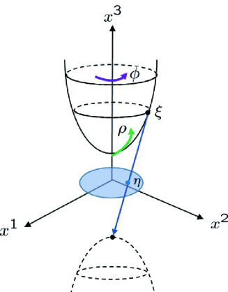
Figure 1: The upper-leaf of Bloch two-hyperboloid $H^{2,0}$ : $-(x^{1})^{2}-(x^{2})^{2}+(x^{3})^{2}=1$. The regions of the parameters are $\rho\in[0,\infty)$ and $\phi\in[0,2\pi)$ realizing $H^{2,0}\simeq\mathbb{R}_{+}\otimes S^{1}$ (29a). The blue shaded region stands for the Poincaré disc.

In (80), the $U(1)$ fibre part $e^{i\frac{\chi}{2}\tau^{3}}$ represents the gauge degrees of freedom. Following the terminology of the $SU(2)$ case [57, 58], we refer to the gauge $\chi=\phi$ as the Dirac-type and $\chi=0$ as the Schwinger-type. The Dirac-type $SU(1,1)$ element corresponds to the squeeze matrix as demonstrated by (83). Meanwhile for the Schwinger-type, we introduce a new squeeze matrix

$$\mathcal{M}(\rho,\phi)\equiv g(\phi,-\rho,0)=e^{i\frac{\phi}{2}\tau^{z}}\cdot e^{i\frac{\rho}{2}\tau^{x}}=\begin{pmatrix}\cosh\frac{\rho}{2}~{}e^{i\frac{\phi}{2}}&-\sinh\frac{\rho}{2}~{}e^{i\frac{\phi}{2}}\\ -\sinh\frac{\rho}{2}~{}e^{-i\frac{\phi}{2}}&\cosh\frac{\rho}{2}~{}e^{-i\frac{\phi}{2}}\end{pmatrix}.$$ (84)

Using the non-compact Hopf spinors [46]

$$\psi_{L}=\frac{1}{\sqrt{2(x^{3}+1)}}\begin{pmatrix}x^{3}+1\\ x^{2}-ix^{1}\end{pmatrix},~{}~{}~{}\psi_{R}=\sigma_{x}{\psi_{L}}^{*}=\frac{1}{\sqrt{2(x^{3}+1)}}\begin{pmatrix}x^{2}+ix^{1}\\ x^{3}+1\end{pmatrix},$$ (87)

which satisfy ${\psi_{L}}^{\dagger}\kappa^{i}\psi_{L}={\psi_{R}}^{\dagger}\kappa^{i}\psi_{R}=x^{i}$, the Dirac-type squeeze matrix (83) can be represented as

$$M=\begin{pmatrix}\psi_{L}&\psi_{R}\end{pmatrix}.$$ (88)

Both $M$ and $\mathcal{M}$ are pseudo-unitary matrices:

$$M(\rho,\phi)^{-1}=\sigma_{z}~{}M(\rho,\phi)^{\dagger}~{}\sigma_{z}=M(-\rho,\phi),$$ (89a)

$$\mathcal{M}(\rho,\phi)^{-1}=\sigma_{z}~{}\mathcal{M}(\rho,\phi)^{\dagger}~{}\sigma_{z}\neq\mathcal{M}(-\rho,\phi).$$ (89b)

The replacement of the non-Hermitian matrices $t^{i}$ with the Hermitian operators $T^{i}$ transforms the squeeze matrix $M$ to the (usual) Dirac-type squeeze operator [23, 24, 25]:

$$S(\xi)=e^{-\xi T^{+}+\xi^{*}T^{-}}=e^{i\phi T^{3}}e^{i\rho T^{1}}e^{-i\phi T^{3}},$$ (90)

which satisfies

$$S(\xi)^{\dagger}=S(-\xi)=S(\xi)^{-1}.$$ (91)

In deriving a number state expansion of the squeezed state, the Gauss decomposition is quite useful [3]. The Gauss decomposition of the $Sp(2;\mathbb{R})$ squeeze operator is given by

$$S(\xi)=e^{-\eta T^{+}}~{}e^{\ln(1-|\eta|^{2})T^{3}}~{}e^{\eta^{*}T^{-}}=e^{-\eta T^{+}}e^{-2\ln(\cosh\frac{\rho}{2})~{}T^{3}}e^{\eta^{*}T^{-}}.$$ (93)

Here, $\eta$ is

$$\eta\equiv\tanh|\xi|~{}\frac{\xi}{|\xi|}=\tanh\frac{\rho}{2}~{}e^{i\phi}=\frac{x^{2}+ix^{1}}{1+x^{3}},$$ (94)

which also has a geometric meaning as the stereographic coordinates on the Poincaré disc from $H^{2,0}$ (see Fig.1).

3.3 Squeezed states

We introduce the squeeze operator corresponding to the Schwinger-type squeeze matrix $\mathcal{M}$ (84) :

$$\mathcal{S}(\xi)=e^{i{\phi}T^{3}}e^{i\rho T^{1}},$$ (95)

which is a unitary operator

$$\mathcal{S}(\xi)^{\dagger}=\mathcal{S}(\xi)^{-1}\neq\mathcal{S}(-\xi).$$ (96)

The Gauss decomposition is derived as

$$\mathcal{S}(\xi)=e^{-\eta T^{+}}e^{(\ln(1-|\eta|^{2})+i\text{arg}(\eta))T^{3}}e^{|\eta|T^{-}}=e^{-\eta T^{+}}e^{-2\ln(\cosh\frac{\rho}{2})~{}T^{3}+i\phi~{}T^{3}}e^{|\eta|T^{-}}.$$ (97)

The two types of the squeeze operator, (90) and (95), are related as

$$S(\xi)=\mathcal{S}(\xi)~{}e^{-i\phi T^{z}}.$$ (98)

In literature, the Dirac-type squeeze operator $S$ is usually adopted, but there may be no special reason not to adopt $\mathcal{S}$, since at the level of non-unitary squeeze matrix, both $M$ and $\mathcal{M}$ denote the coset $H^{2,0}$.

Since $T^{z}$ is diagonalized for the number-basis states, the one-mode Dirac- and Schwinger-type squeezed number states

$$|\xi\rangle_{(n)}\equiv S(\xi)|n\rangle,~{}~{}~{}~{}~{}|\xi\rangle\!\rangle_{(n)}\equiv\mathcal{S}(\xi)|n\rangle,$$ (100)

are merely different by a $U(1)$ phase:

$$|\xi\rangle_{(n)}=e^{-i\frac{\phi}{4}}e^{-i\frac{\phi}{2}n}\cdot|\xi\rangle\!\rangle_{(n)},$$ (101)

where $|n\rangle=\frac{1}{\sqrt{n!}}{a^{\dagger}}^{n}|0\rangle.$ Similarly for two-mode, the squeezed number states are related as

$$|\xi\rangle_{(n_{a},n_{b})}=e^{-i\frac{\phi}{2}}e^{-i\frac{\phi}{2}(n_{a}+n_{b})}\cdot|\xi\rangle\!\rangle_{(n_{a},n_{b})}$$ (104)

where

$$|\xi\rangle_{(n_{a},n_{b})}\equiv S(\xi)|n_{a},n_{b}\rangle,~{}~{}~{}~{}~{}|\xi\rangle\!\rangle_{(n_{a},n_{b})}\equiv\mathcal{S}(\xi)|n_{a},n_{b}\rangle,$$ (105)

with $|n_{a},n_{b}\rangle=\frac{1}{\sqrt{n_{a}!n_{b}!}}{a^{\dagger}}^{n_{a}}{b^{\dagger}}^{n_{b}}|0,0\rangle.$ As the overall phase has nothing to do with the physics, the two type squeezed number states are physically identical.

Next, we consider the squeezed coherent state [22, 23, 24]. Since the coherent state is a superposition of number states

$$|\alpha\rangle=e^{\frac{1}{2}|\alpha|^{2}}\sum_{n=0}^{\infty}\frac{1}{\sqrt{n!}}\alpha^{n}|n\rangle,$$ (106)

the squeezed coherent state can be expressed by the superposition of the squeezed number states :

$$|\xi,\alpha\rangle\equiv S(\xi)|\alpha\rangle=e^{\frac{1}{2}|\alpha|^{2}}\sum_{n=0}^{\infty}\frac{1}{\sqrt{n!}}\alpha^{n}|\xi\rangle_{n},~{}~{}~{}~{}~{}~{}~{}|\xi,\alpha\rangle\!\rangle\equiv\mathcal{S}(\xi)|\alpha\rangle=e^{\frac{1}{2}|\alpha|^{2}}\sum_{n=0}^{\infty}\frac{1}{\sqrt{n!}}\alpha^{n}|\xi\rangle\!\rangle_{(n)}.$$ (107)

Recall that the Dirac-type squeezed number states and the Schwinger-type only differ by the $U(1)$ factor depending on the number $n$ (101), so we obtain the relation between the squeezed coherent states of the Dirac-type and Schwinger-type as

$$|\xi,\alpha_{D}\rangle=e^{-i\frac{\phi}{4}}|\xi,\alpha_{S}\rangle\!\rangle$$ (108)

with

$$\alpha_{{D}}=\alpha_{S}e^{-i\frac{\phi}{2}}.$$ (109)

The Dirac- and Schwinger-type squeezed coherent states represent superficially different physical states except for the squeezed vacuum case $\alpha_{S}=\alpha_{D}=0$. However as implied by (109), the difference between the two type squeezed states can be absorbed in the phase part of the displacement parameter $\alpha$. Since the displacement parameter indicates the position of the squeezed coherent state on the $x^{1}$-$x^{2}$ plane [26, 27], the elliptical uncertainty regions representing the two squeezed coherent states on the $x^{1}$-$x^{2}$ plane merely differ by the rotation $\frac{\phi}{2}$. This is also suggested by the $U(1)$ part $e^{i{\phi}T^{3}}$ of (90), which denotes the rotation around the $x^{3}$-axis. Similarly for the two-modes, the Dirac- [26, 27] and Schwinger-type squeezed coherent states

$$|\xi,\alpha,\beta\rangle\equiv S(\xi)|\alpha,\beta\rangle=e^{\frac{1}{2}(|\alpha|^{2}+|\beta|^{2})}\sum_{n_{a},n_{b}}\frac{1}{\sqrt{n_{a}!n_{b}!}}~{}\alpha^{n_{a}}\beta^{n_{b}}|\xi\rangle_{(n_{a},n_{b})},$$

$$|\xi,\alpha,\beta\rangle\!\rangle\equiv\mathcal{S}(\xi)|\alpha,\beta\rangle=e^{\frac{1}{2}(|\alpha|^{2}+|\beta|^{2})}\sum_{n_{a},n_{b}}\frac{1}{\sqrt{n_{a}!n_{b}!}}~{}\alpha^{n_{a}}\beta^{n_{b}}|\xi\rangle\!\rangle_{(n_{a},n_{b})},$$ (110)

are related as

$$|\xi,\alpha_{D},\beta_{D}\rangle=e^{-i\frac{\phi}{2}}~{}|\xi,\alpha_{S},\beta_{S}\rangle\!\rangle$$ (111)

with

$$\alpha_{D}=\alpha_{S}e^{-i\frac{\phi}{2}},~{}~{}\beta_{D}=\beta_{S}e^{-i\frac{\phi}{2}}.$$ (112)

4 $Sp(4;\mathbb{R})$ squeeze matrices and the non-compact 2nd Hopf map

The next-simple symplectic group is $Sp(4;\mathbb{R})$. Among the real symplectic groups, only $Sp(2;\mathbb{R})$ and $Sp(4;\mathbb{R})$ are isomorphic to indefinite spin groups;

$$Sp(2;\mathbb{R})\simeq Spin(2,1),~{}~{}~{}~{}Sp(4;\mathbb{R})\simeq Spin(2,3).$$ (113)

Futhermore, the $SO(2,3)$ group is the isometry group of the four-hyperboloid with split-signature, $H^{2,2}$, – the basemanifold of the non-compact 2nd Hopf map. Encouraged by these mathematical analogies, we explore an $Sp(4;\mathbb{R})$ extension of the previous $Sp(2;\mathbb{R})$ analysis. For details of $Sp(4;\mathbb{R})$ group, one may consult with Ref.[61] for instance.

4.1 $sp(4;\mathbb{R})$ algebra

From the result of Sec.2.2, we see

$$Mp(4;\mathbb{R})/\mathbb{Z}_{2}~{}\simeq~{}Sp(4;\mathbb{R})~{}\simeq~{}Spin(2,3)~{}\simeq~{}S^{1}\times S^{3}\times\mathbb{R}^{6}.$$ (114)

The metaplectic group $Mp(4,\mathbb{R})$ is the double cover of the symplectic group $Sp(4,\mathbb{R})$. As the metaplectic representation of $Sp(2;\mathbb{R})$ is constructed by the Majorana representation of $SO(2,1)$, the $SO(2,3)$ Majorana representation is expected to realize the $Sp(4;\mathbb{R})$ metaplectic representation.

The $sp(4;\mathbb{R})$ algebra is isomorphic to $so(2,3)$ algebra (Appendix B.3), which consists of ten generators $T^{ab}=-T^{ba}$ $(a,b=1,2,\cdots,5)$:

$$[T^{ab},T^{cd}]=ig^{ac}T^{bd}-ig^{ad}T^{bc}+ig^{bd}T^{ac}-ig^{bc}T^{ad}$$ (115)

where

$$g_{ab}=g^{ab}=\text{diag}(-1,-1,+1,+1,+1).$$ (116)

The quadratic $SO(2,3)$ Casimir operator is given by

$$C =\sum_{a<b=1}^{5}T^{ab}~{}T_{ab}$$

$$=(T^{12})^{2}-(T^{13})^{2}-(T^{14})^{2}-(T^{15})^{2}-(T^{23})^{2}-(T^{24})^{2}-(T^{25})^{2}+(T^{34})^{2}+(T^{35})^{2}+(T^{45})^{2}.$$ (117)

It is not difficult to construct non-Hermitian matrix realization of the $so(2,3)$ generators. For this purpose, we first introduce the $SO(2,3)$ gamma matrices $\gamma^{a}$ that satisfy

$$\{\gamma^{a},\gamma^{b}\}=2g^{ab}.$$ (118)

Placing the split-quaternion (39) and its conjugate (40) in the off-diagonal components of gamma matrices, we can construct the $SO(2,3)$ gamma matrices as

$$\gamma^{a}=\{\gamma^{m},\gamma^{5}\}=\{\begin{pmatrix}0&\bar{q}^{m}\\ q^{m}&0\end{pmatrix},~{}~{}\begin{pmatrix}1&0\\ 0&-1\end{pmatrix}\}$$ (119)

or

$$\gamma^{i}=\begin{pmatrix}0&i\tau^{i}\\ -i\tau^{i}&0\end{pmatrix},~{}~{}\gamma^{4}=\begin{pmatrix}0&1\\ 1&0\end{pmatrix},~{}~{}\gamma^{5}=\begin{pmatrix}1&0\\ 0&-1\end{pmatrix}.$$ (120)

Notice that $\gamma^{a}$ are pseudo-Hermitian:

$${\gamma^{a}}^{\dagger}=\gamma_{a}=k\gamma^{a}k,$$ (121)

where

$$k\equiv i\gamma^{1}\gamma^{2}=\begin{pmatrix}\sigma_{z}&0\\ 0&\sigma_{z}\end{pmatrix}.$$ (122)

The corresponding $so(2,3)$ matrices, $\sigma^{ab}=-i\frac{1}{4}[\gamma^{a},\gamma^{b}]$, are derived as

$$\sigma^{mn}=-\frac{1}{2}\begin{pmatrix}\bar{\eta}^{mni}\tau_{i}&0\\ 0&{\eta}^{mni}\tau_{i}\end{pmatrix},~{}~{}~{}\sigma^{i5}=-\frac{1}{2}\begin{pmatrix}0&\tau^{i}\\ \tau^{i}&0\end{pmatrix},~{}~{}\sigma^{45}=i\frac{1}{2}\begin{pmatrix}0&1\\ -1&0\end{pmatrix}.$$ (123)

Here, $\eta^{mni}$ and $\bar{\eta}^{mni}$ denote the ’t Hooft symbols with the split signature:

$$\eta_{mni}=\epsilon_{mni4}+g_{mi}g_{n4}-g_{ni}g_{m4},~{}~{}~{}\bar{\eta}_{mni}=\epsilon_{mni4}-g_{mi}g_{n4}+g_{ni}g_{m4}.$$ (124)

The $so(2,3)$ matices are also pseudo-hermitian :

$$(\sigma^{ab})^{\dagger}=\sigma_{ab}=k\sigma^{ab}k.$$ (125)

Obviously $k$ is unitarily equivalent to $K=\begin{pmatrix}1_{2}&0\\ 0&-1_{2}\end{pmatrix}$ for $Sp(4;\mathbb{R})$. From the general discussion of Sec.2, the corresponding Hermitian matrices are given by

$$k^{a}\equiv k\gamma^{a}={k^{a}}^{\dagger},~{}~{}~{}~{}~{}k^{ab}\equiv k\sigma^{ab}={k^{ab}}^{\dagger},$$ (129)

and the Hermitian operators are

$$X^{a}=\hat{\psi}^{\dagger}~{}k^{a}~{}\hat{\psi},~{}~{}~{}~{}X^{ab}=\hat{\psi}^{\dagger}~{}k^{ab}~{}\hat{\psi},$$ (130)

where $\hat{\psi}$ denotes a four-component operator whose components satisfy

$$[\hat{\psi}_{\alpha},\hat{\psi}_{\beta}^{\dagger}]=k_{\alpha\beta}.~{}~{}~{}~{}~{}(\alpha,\beta=1,2,3,4)$$ (131)

We can explicitly realize $\hat{\psi}$ as

$$\hat{\psi}=\begin{pmatrix}a&b^{\dagger}&c&d^{\dagger}\end{pmatrix}^{t}.$$ (132)

Here, $a$, $b$, $c$ and $d$ are independent Schwinger boson operators, $i.e.$ $[a,a^{\dagger}]=[b,b^{\dagger}]=[c,c^{\dagger}]=[d,d^{\dagger}]=1$ and $[a,b^{\dagger}]=[a,c]=[c,d^{\dagger}]=\cdots=0.$ $X^{a}$ and $X^{ab}$ (130) read as

$$X^{1}=-a^{\dagger}d^{\dagger}+bc-ad+b^{\dagger}c^{\dagger},~{}~{}X^{2}=ia^{\dagger}d^{\dagger}+ibc-iad-ib^{\dagger}c^{\dagger},~{}~{}X^{3}=ia^{\dagger}c+id^{\dagger}b-ic^{\dagger}a-ib^{\dagger}d,$$

$$X^{4}=a^{\dagger}c-d^{\dagger}b+c^{\dagger}a-b^{\dagger}d,~{}~{}~{}X^{5}=a^{\dagger}a-bb^{\dagger}-c^{\dagger}c+dd^{\dagger}=a^{\dagger}a-b^{\dagger}b-c^{\dagger}c+d^{\dagger}d,$$ (133)

and

$$X^{12}=-\frac{1}{2}(a^{\dagger}a+bb^{\dagger}+c^{\dagger}c+dd^{\dagger}),~{}~{}X^{13}=-\frac{1}{2}(a^{\dagger}b^{\dagger}+ab+c^{\dagger}d^{\dagger}+cd),~{}~{}X^{14}=i\frac{1}{2}(a^{\dagger}b^{\dagger}-ab-c^{\dagger}d^{\dagger}+cd),$$

$$X^{15}=i\frac{1}{2}(-a^{\dagger}d^{\dagger}+ad-b^{\dagger}c^{\dagger}+bc),~{}~{}X^{23}=i\frac{1}{2}(a^{\dagger}b^{\dagger}-ab+c^{\dagger}d^{\dagger}-cd),~{}~{}~{}X^{24}=\frac{1}{2}(a^{\dagger}b^{\dagger}+ab-c^{\dagger}d^{\dagger}-cd),$$

$$X^{25}=-\frac{1}{2}(a^{\dagger}d^{\dagger}+ad+b^{\dagger}c^{\dagger}+bc),~{}~{}~{}X^{34}=\frac{1}{2}(a^{\dagger}a+bb^{\dagger}-c^{\dagger}c-dd^{\dagger}),~{}~{}~{}~{}X^{35}=-\frac{1}{2}(a^{\dagger}c+ac^{\dagger}+d^{\dagger}b+db^{\dagger}),$$

$$X^{45}=i\frac{1}{2}(a^{\dagger}c-c^{\dagger}a-d^{\dagger}b+b^{\dagger}d).$$ (134)

With (133) and (134), we can show

$$\sum_{a=1}^{5}X^{a}X_{a}=(\bar{\hat{\psi}}\hat{\psi}+2)(\bar{\hat{\psi}}\hat{\psi}-2),~{}~{}~{}~{}~{}\sum_{a>b=1}^{5}X^{ab}X_{ab}=\frac{1}{2}(\bar{\hat{\psi}}\hat{\psi})(\bar{\hat{\psi}}\hat{\psi}+6)+1,$$ (135)

where

$$\bar{\hat{\psi}}\hat{\psi}\equiv\hat{\psi}^{\dagger}k\hat{\psi}=a^{\dagger}a-b^{\dagger}b+c^{\dagger}c-d^{\dagger}d-2.$$ (136)

$\bar{\hat{\psi}}\hat{\psi}$ is a singlet under the $SU(2,2)$ transformation:

$$[X^{a},\bar{\hat{\psi}}\hat{\psi}]=[X^{ab},\bar{\hat{\psi}}\hat{\psi}]=0,$$ (137)

and the sixteen operators, $X^{a}$, $X^{ab}$ and $\bar{\psi}\psi$, constitute the $u(2,2)$ algebra.

As we shall see below, the Majorana representation of $SO(2,3)$ realizes the metaplectic representation of $Sp(4;\mathbb{R})$. The $SO(2,3)$ group has the charge conjugation matrix satisfying

$$-(\sigma^{ab})^{*}=C\sigma^{ab}C,$$ (138)

where

$$C=\begin{pmatrix}\sigma_{x}&0\\ 0&\sigma_{x}\end{pmatrix}.$$ (139)

The $SO(2,3)$ Majorana spinor operator subject to the Majorana condition

$$\hat{\psi}^{*}=C\hat{\psi}$$ (140)

is given by

$$\hat{\psi}_{\text{M}}=\begin{pmatrix}a&a^{\dagger}&b&b^{\dagger}\end{pmatrix}^{t}$$ (141)

whose components satisfy the commutation relations

$$[\hat{\psi}_{\text{M}\alpha},\hat{\psi}_{\text{M}\beta}]=\mathcal{E}_{\alpha\beta}$$ (142)

with

$$\mathcal{E}=kC=-Ck=\begin{pmatrix}i\sigma_{y}&0\\ 0&i\sigma_{y}\end{pmatrix}.$$ (143)

Just as in the case of $SO(2,1)$ (60), using $\mathcal{E}$, we can introduce symmetric matrices

$$m^{ab}\equiv-\mathcal{E}\sigma^{ab},~{}~{}~{}~{}((m^{ab})^{t}=m^{ab})$$ (144)

to construct the $so(2,3)$ generators

$$X^{ab}\equiv\frac{1}{2}{\hat{\psi}_{\text{M}}}^{t}~{}m^{ab}~{}\hat{\psi}_{\text{M}},$$ (145)

which are

$$X^{12}=-\frac{1}{2}(a^{\dagger}a+bb^{\dagger})=-\frac{1}{2}(a^{\dagger}a+b^{\dagger}b+1),~{}~{}~{}X^{13}=-\frac{1}{4}(a^{2}+{a^{\dagger}}^{2}+b^{2}+{b^{\dagger}}^{2}),$$

$$X^{14}=i\frac{1}{4}(-a^{2}+{a^{\dagger}}^{2}+b^{2}-{b^{\dagger}}^{2}),~{}~{}~{}X^{15}=i\frac{1}{2}(ab-a^{\dagger}b^{\dagger}),~{}~{}~{}X^{23}=i\frac{1}{4}(-a^{2}+{a^{\dagger}}^{2}-b^{2}+{b^{\dagger}}^{2}),$$

$$X^{24}=\frac{1}{4}(a^{2}+{a^{\dagger}}^{2}-b^{2}-{b^{\dagger}}^{2}),~{}~{}~{}~{}X^{25}=-\frac{1}{2}(ab+a^{\dagger}b^{\dagger}),~{}~{}~{}X^{34}=\frac{1}{2}(a^{\dagger}a-b^{\dagger}b),$$

$$X^{35}=-\frac{1}{2}(a^{\dagger}b+ab^{\dagger}),~{}~{}~{}~{}X^{45}=i\frac{1}{2}(a^{\dagger}b-b^{\dagger}a).$$ (146)

Comparing the Majorana representation generators (145) with the Dirac representation generators (130), one can find the coefficient on the right-hand side of (145) is half of that of (130) just as in the case of the $Sp(2;\mathbb{R})$ and $Mp(2;\mathbb{R})$. This implies that (145) are the generators of the double covering group of $Sp(4;\mathbb{R})$, which is $Mp(4;\mathbb{R})$.

We also construct antisymmetric matrices (370) as

$$m^{a}\equiv\mathcal{E}\gamma^{a}.$$ (147)

One can easily check that the corresponding operators identically vanish:

$$X^{a}\equiv{\hat{\psi}_{\text{M}}}^{t}~{}m^{a}~{}\hat{\psi}_{\text{M}}=0.$$ (148)

The $U(2,2)$ completeness relation is represented as

$$(m^{a})_{\alpha\beta}(m_{a})_{\gamma\delta}+4\sum_{a<b}(m^{ab})_{\alpha\beta}(m_{ab})_{\gamma\delta}=-4\mathcal{E}_{\alpha\delta}\mathcal{E}_{\beta\gamma}-\mathcal{E}_{\alpha\beta}\mathcal{E}_{\gamma\delta}.$$ (149)

Using (149) and (148), we can show that the corresponding $SO(2,3)$ Casimir becomes a constant:

$$\sum_{a>b=1}^{5}X^{ab}~{}X_{ab}=-\frac{5}{4},$$ (150)

where we used $\mathcal{E}_{\alpha\beta}(\psi_{\text{M}})_{\alpha}(\psi_{\text{M}})_{\beta}=[a,a^{\dagger}]+[b,b^{\dagger}]=2$. (150) should be compared with the previous $SU(1,1)$ result (64). Notice that the independent operators of (146) are simply given by the symmetric combination of the two-mode operators $a_{i}=a,b$ :

$$\{a_{i},a_{j}\},~{}~{}~{}\{a_{i}^{\dagger},a_{j}^{\dagger}\},~{}~{}\{a_{i},a_{j}^{\dagger}\},$$ (151)

which are known to realize the generators of $Mp(4;\mathbb{R})$ (see Appendix A.3). Also from this observation, one may see that (145) realizes $mp(4;\mathbb{R})$ generators. There are two $SO(2,3)$ metaplectic irreducible representations referred to as the singletons with the Casimir (150) [62].

4.2 Gauss decomposition

In the $Sp(2;\mathbb{R})$ case, we used the coset representation of $H^{2,0}$

$$H^{2,0}~{}\simeq~{}SO(2,1)/SO(2)~{}\simeq~{}SU(1,1)/U(1)~{}\simeq~{}Sp(2,\mathbb{R})/U(1),$$ (152)

which is equivalent to the 1st non-compact Hopf map

$$H^{2,0}~{}\simeq~{}H^{2,1}/S^{1}.$$ (153)

In the $Sp(4;\mathbb{R})$ case, the corresponding coset is obviously given by

$$H^{2,2} ~{}\simeq~{}SO(2,3)/SO(2,2)$$

$$~{}\simeq~{}SO(2,3)/(SU(1,1)_{L}\otimes SU(1,1)_{R})~{}\simeq~{}Sp(4,\mathbb{R})/(Sp(2;\mathbb{R})_{L}\otimes Sp(2;\mathbb{R})_{R}),$$ (154)

which is the basemanifold of the 2nd non-compact Hopf map

$$H^{2,2}~{}\simeq~{}H^{4,3}/H^{2,1}.$$ (155)

The coordinates $x^{a}$ $(a=1,2,3,4,5)$ on $H^{2,2}$ should satisfy

$$\sum_{a,b}g_{ab}x^{a}x^{b}=-x^{1}x^{1}-x^{2}x^{2}+x^{3}x^{3}+x^{4}x^{4}+x^{5}x^{5}=1.$$ (156)

We parameterize $x^{a}$ as

$$x^{m}=(x^{1},x^{2},x^{3},x^{4})=(\sin\theta\cos\chi\sinh\rho,~{}\sin\theta\sin\chi\sinh\rho,~{}\sin\theta\cos\phi\cosh\rho,~{}\sin\theta\sin\phi\cosh\rho),$$

$$x^{5}=\cos\theta,$$ (157)

where the ranges of the parameters are given by (see Fig.2)

$$\rho,\theta~{}\in~{}\mathbb{R}_{+}\times S^{1}\simeq H^{1,1},~{}~{}~{}\chi,\phi~{}\in~{}S^{1}\times S^{1}.$$ (158)

As we have called $H^{2,0}$ associated with the $Sp(2;\mathbb{R})$ squeeze operator the Bloch two-hyperboloid, we will refer to $H^{2,2}$ as the Bloch four-hyperboloid in the following.

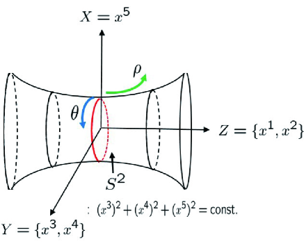
Figure 2: Bloch four-hyperboloid $H^{2,2}$ : $-((x^{1})^{2}+(x^{2})^{2})+((x^{3})^{2}+(x^{4})^{2})+(x^{5})^{2}=1$. The Bloch four-hyperboloid can be regarded as a one-sheet hyperboloid $-Z^{2}+Y^{2}+X^{2}=1$ with $Z=(x^{1},x^{2})$, $Y=(x^{3},x^{4})$ and $X=x^{5}$. Each of the dimensions $Z$ and $Y$ has an internal $S^{1}$ structure. In the parametrization (157) the range of $x^{5}$ is $[-1,1]$, meaning that the parameterization does not cover the whole surface of the Bloch four-hyperboloid.

We also introduce “normalized” coordinates

$$y^{m}=(\cos\chi\sinh\rho,~{}\sin\chi\sinh\rho,~{}\cos\phi\cosh\rho,~{}\sin\phi\cosh\rho)$$ (159)

which satisfy $y^{m}y_{m}=-y^{1}y^{1}-y^{2}y^{2}+y^{3}y^{3}+y^{4}y^{4}=1$ and denote the $H^{2,1}$-latitude of the Bloch four-hyperboloid with fixed $\theta$.

Based on the $G/H$ construction (154), we can easily derive a $Sp(4;\mathbb{R})$ squeeze matrix representing $H^{2,2}$. We take $\sigma^{mn}$, as the generators of $SO(2,2)$ group and $\sigma^{m5}=\begin{pmatrix}0&-\bar{q}^{m}\\ q^{m}&0\end{pmatrix}$ as the broken four generators. The squeeze matrix for $H^{2,2}$ is then given by

$$M =e^{i\theta~{}y_{m}\sigma^{m5}}=\begin{pmatrix}\cos\frac{\theta}{2}~{}1_{2}&-\sin\frac{\theta}{2}~{}y^{m}\bar{q}_{m}\\ \sin\frac{\theta}{2}~{}y^{m}{q}_{m}&\cos\frac{\theta}{2}~{}1_{2}\end{pmatrix}=\frac{1}{\sqrt{2(1+x^{5})}}\begin{pmatrix}(1+x^{5})1_{2}&-\bar{q}_{m}x^{m}\\ q_{m}x^{m}&(1+x^{5})1_{2}\end{pmatrix}.$$ (160)

In the polar coordinates, (160) is expressed as

$$M=\begin{pmatrix}\cos\frac{\theta}{2}&0&-i\sin\frac{\theta}{2}~{}\cosh\rho~{}e^{-i\phi}&-\sin\frac{\theta}{2}~{}\sinh\rho~{}e^{-i\chi}\\ 0&\cos\frac{\theta}{2}&-\sin\frac{\theta}{2}~{}\sinh\rho~{}e^{i\chi}&i\sin\frac{\theta}{2}~{}\cosh\rho~{}e^{i\phi}\\ -i\sin\frac{\theta}{2}~{}\cosh\rho~{}e^{i\phi}&-\sin\frac{\theta}{2}~{}\sinh\rho~{}e^{-i\chi}&\cos\frac{\theta}{2}&0\\ -\sin\frac{\theta}{2}~{}\sinh\rho~{}e^{i\chi}&i\sin\frac{\theta}{2}~{}\cosh\rho~{}e^{-i\phi}&0&\cos\frac{\theta}{2}\end{pmatrix}.$$ (161)

It is also possible to derive the $Sp(4;\mathbb{R})$ squeeze matrix (160) based on the 2nd non-compact Hopf map (155). This construction will be important in the Euler angle decomposition [Sec.4.3]. The 2nd non-compact Hopf map is explicitly given by [46]

$$\psi~{}\in H^{4,3}~{}\rightarrow~{}x^{a}=\psi^{\dagger}k^{a}\psi~{}\in~{}H^{2,2},$$ (162)

where $\psi$ is subject to

$$\psi^{\dagger}k\psi=(\psi_{1}^{*}\psi_{1}+\psi_{3}^{*}\psi_{3})-(\psi_{2}^{*}\psi_{2}+\psi_{4}^{*}\psi_{4})=1,$$ (163)

and $x^{a}$ (162) automatically satisfy the condition of $H^{2,2}$:

$$g_{ab}x^{a}x^{b}=(\psi^{\dagger}k\psi)^{2}=1.$$ (164)

We can express $\psi$ as

$$\psi=\Psi_{L}h\begin{pmatrix}1\\ 0\end{pmatrix}=\Psi_{L}\phi$$ (165)

where $\Psi_{L}$ denotes the following $4\times 2$ matrix

$$\Psi_{L}\equiv\frac{1}{\sqrt{2(1+x^{5})}}\begin{pmatrix}(1+x^{5})1_{2}\\ q_{m}x^{m}\end{pmatrix},$$ (169)

and $h$ is an arbitrary $SU(1,1)$ group element representing a $H^{2,1}$-fibre:

$$h=\begin{pmatrix}\phi&\sigma_{x}\phi^{*}\end{pmatrix}=\begin{pmatrix}\phi_{1}&\phi_{2}^{*}\\ \phi_{2}&\phi_{1}^{*}\end{pmatrix}$$ (170)

subject to

$$\det h=|\phi_{1}|^{2}-|\phi_{2}|^{2}=\phi^{\dagger}\sigma_{z}\phi=1.$$ (171)

$\Psi_{L}$ is an eigenstate of the $x^{a}\gamma_{a}$ with positive chirality

$$x^{a}\gamma_{a}\Psi_{L}=+\Psi_{L}.$$ (172)

Similarly, a negative chirality matrix satisfying

$$x^{a}\gamma_{a}\Psi_{R}=-\Psi_{R}$$ (173)

is given by

$$\Psi_{R}=\frac{1}{\sqrt{2(1+x^{5})}}\begin{pmatrix}-\bar{q}_{m}x^{m}\\ (1+x^{5})1_{2}\end{pmatrix}.$$ (174)

With these two opposite chirality matrices, $M$ (160) can be simply expressed as

$$M=\begin{pmatrix}\Psi_{L}&\Psi_{R}\end{pmatrix}.$$ (175)

(See Appendix C for more details about relations between the squeeze matrix and the non-compact Hopf spinors.)

Here, we mention the Gauss decomposition of $M$. Following to the general method of [60], we may in principle derive the normal ordering of $M$. However, for the $Sp(4;\mathbb{R})$ group the ten generators are concerned, and the Gauss decomposition will be a formidable task. Therefore instead of attempting the general method, we resort to an intuitive geometric structure of the Hopf maps to derive the Gauss decomposition. The hierarchical geometry of the Hopf maps implies that the $U(1)$ part of the 1st non-compact Hopf map will be replaced with the $SU(1,1)$ group in the 2nd. We then expect that the Gauss decomposition of $M$ will be given by

$$M =\text{Exp}\biggl{(}{-\tan\frac{\theta}{2}~{}\begin{pmatrix}0&y^{m}\bar{q}_{m}\\ 0&0\end{pmatrix}}\biggr{)}\cdot\text{Exp}\biggl{(}{-\ln\biggl{(}\cos\frac{\theta}{2}\biggr{)}~{}\begin{pmatrix}1_{2}&0\\ 0&-1_{2}\end{pmatrix}}\biggr{)}\cdot\text{Exp}\biggl{(}{\tan\frac{\theta}{2}~{}\begin{pmatrix}0&0\\ y^{m}{q}_{m}&0\end{pmatrix}}\biggr{)}$$

$$=\text{Exp}\biggl{(}-\tan\frac{\theta}{2}~{}y^{m}\cdot(\frac{1}{2}\gamma_{m}-i\sigma_{m5})\biggr{)}\cdot\text{Exp}\biggl{(}-\ln\biggl{(}\cos\frac{\theta}{2}\biggr{)}~{}\gamma^{5}\biggr{)}\cdot\text{Exp}\biggl{(}\tan\frac{\theta}{2}~{}y^{m}\cdot(\frac{1}{2}\gamma_{m}+i\sigma_{m5})\biggr{)}.$$ (176)

Substituting the matrices, we can demonstrate the validity of (176). Notice that, unlike the $Sp(2;\mathbb{R})$ case (93), the Gauss decomposition (176) cannot be expressed only within the ten generators of $Sp(4;\mathbb{R})$, but we need to utilize the five $SO(2,3)$ gamma matrices as well. The fifteen matrices made of the $SO(2,3)$ gamma matrices and generators amount to the $so(2,4)\simeq su(2,2)$ algebra.

4.3 Euler angle decomposition

Here we derive Euler angle decomposition of the $Sp(4;\mathbb{R})$ squeeze matrix based on the hierarchical geometry of the non-compact Hopf maps. The Euler decomposition is crucial to perform the number state expansion of $Sp(4;\mathbb{R})$ squeezed states.

We first introduce a dimensionality reduction of the 2nd non-compact Hopf map, which we refer to as the non-compact chiral Hopf map:

$$H^{2,1}_{L}\otimes H^{2,1}_{R}~{}~{}\overset{H^{2,1}_{\text{diag.}}}{\longrightarrow}~{}~{}H^{2,1}.$$ (177)

(177) is readily obtained by imposing one more constraint to the non-compact 2nd Hopf spinor:

$$\psi^{\dagger}k^{5}\psi=1,$$ (178)

in addition to the original constraint (163). When we denote the non-compact Hopf spinor as $\psi=(\psi_{L}~{}~{}\psi_{R})^{t}$ the two constraints, (163) and (178), are rephrased as “normalizations” for each of the two-component chiral Hopf spinors,

$${\psi_{L}}^{\dagger}\sigma_{z}\psi_{L}=1,~{}~{}~{}{\psi_{R}}^{\dagger}\sigma_{z}\psi_{R}=1.$$ (179)

$\psi_{L}$ and $\psi_{R}$ are thus the coordinates on $H^{2,1}\otimes H^{2,1}$, and (177) is explicitly realized as

$$\psi_{L},~{}\psi_{R}~{}~{}\rightarrow~{}~{}y^{m}=\frac{1}{2}({\psi_{L}}^{\dagger}\sigma_{z}\bar{q}^{m}\psi_{R}+{\psi_{R}}^{\dagger}\sigma_{z}q^{m}\psi_{L}),$$ (180)

and so $y^{m}$ automatically satisfy

$$y^{m}y_{m}=-(y^{1})^{2}-(y^{2})^{2}+(y^{3})^{2}+(y^{4})^{2}=({\psi_{L}}^{\dagger}\sigma_{z}\psi_{L})({\psi_{R}}^{\dagger}\sigma_{z}\psi_{R})=1,$$ (181)

so $y^{m}$ stand for the coordinates on $H^{2,1}$. The simultaneous $SU(1,1)$ transformation of $\psi_{L}$ and $\psi_{R}$ has nothing to do with $y^{m}$ and geometrically represents $H^{2,1}_{\text{diag}}$-fibre part which is projected out in (177).

We can express the chiral Hopf spinors as

$$\psi_{L}=e^{-i\frac{\phi}{2}\sigma_{z}}~{}\begin{pmatrix}\cosh\frac{\rho}{2}~{}e^{-i\frac{1}{2}\chi}\\ -i\sinh\frac{\rho}{2}~{}e^{i\frac{1}{2}\chi}\end{pmatrix},~{}~{}~{}\psi_{R}=-i~{}e^{i\frac{\phi}{2}\sigma_{z}}~{}\begin{pmatrix}\cosh\frac{\rho}{2}~{}e^{-i\frac{1}{2}\chi}\\ -i\sinh\frac{\rho}{2}~{}e^{i\frac{1}{2}\chi}\end{pmatrix},$$ (182)

and the resultant $y^{m}$ from (180) are given by (159). Notice that when $\phi=0$, $\psi_{L}$ and $\psi_{L}$ are reduced to the 1st non-compact Hopf spinor and $y^{m}$ (159) are also reduced to the coordinates on $H^{2,0}$. In this sense, the non-compact chiral Hopf map incorporates the structure of the 1st non-compact Hopf map in a hierarchical manner of dimensions. The $SU(1,1)$ group elements corresponding to $\psi_{L}$ and $\psi_{R}$ are given by

$$H_{L} \equiv\begin{pmatrix}\psi_{L}&\sigma_{x}{\psi_{L}}^{*}\end{pmatrix}=\begin{pmatrix}\cosh\frac{\rho}{2}~{}e^{-i\frac{1}{2}(\chi+\phi)}&i\sinh\frac{\rho}{2}~{}e^{-i\frac{1}{2}(\chi+\phi)}\\ -i\sinh\frac{\rho}{2}~{}e^{i\frac{1}{2}(\chi+\phi)}&\cosh\frac{\rho}{2}~{}e^{i\frac{1}{2}(\chi+\phi)}\end{pmatrix}=e^{-\frac{\rho}{2}\sigma_{y}}~{}e^{-i\frac{1}{2}(\chi+\phi)\sigma_{z}},$$

$$H_{R} \equiv i\begin{pmatrix}\psi_{R}&-\sigma_{x}{\psi_{R}}^{*}\end{pmatrix}=\begin{pmatrix}\cosh\frac{\rho}{2}~{}e^{-i\frac{1}{2}(\chi-\phi)}&i\sinh\frac{\rho}{2}~{}e^{-i\frac{1}{2}(\chi-\phi)}\\ -i\sinh\frac{\rho}{2}~{}e^{i\frac{1}{2}(\chi-\phi)}&\cosh\frac{\rho}{2}~{}e^{i\frac{1}{2}(\chi-\phi)}\end{pmatrix}=e^{-\frac{\rho}{2}\sigma_{y}}~{}e^{-i\frac{1}{2}(\chi-\phi)\sigma_{z}}.$$ (183)

From the chiral Hopf spinors, we can reconstruct a non-compact 2nd Hopf spinor that satisfies the 2nd non-compact Hopf map (162) as

$${\psi^{\prime}}=\begin{pmatrix}\sqrt{\frac{1+x^{5}}{2}}~{}\psi_{L}\\ \sqrt{\frac{1-x^{5}}{2}}~{}\psi_{R}\end{pmatrix}.$$ (184)

($\psi$ (165) and $\psi^{\prime}$ (184) are related by the $SU(1,1)$ gauge transformation as we shall see below.) One may find that the $x^{5}$ coordinate on $H^{2,2}$ determines the weights of the chiral Hopf spinors in $\psi^{\prime}$. In particular at the “north pole” ($x^{5}=1$), $\psi^{\prime}$ (184) is reduced to $\psi_{L}$, while at the “south pole” ($x^{5}=-1$) $\psi_{R}$. The hierarchical geometry of the Hopf maps is summarized as

The 1st Hopf map for $H^{2,0}$   $\rightarrow$   The chiral Hopf map for $H^{2,1}$   $\rightarrow$   The 2nd Hopf map for $H^{2,2}$.

From the chiral Hopf spinors, we construct the following $4\times 2$ matrix

$$\Psi^{\prime}_{L}=\begin{pmatrix}\sqrt{\frac{1+x^{5}}{2}}\begin{pmatrix}\psi_{L}&\sigma_{x}{\psi_{L}}^{*}\end{pmatrix}\\ \sqrt{\frac{1-x^{5}}{2}}\begin{pmatrix}\psi_{R}&\sigma_{x}{\psi_{R}}^{*}\end{pmatrix}\end{pmatrix}.$$ (185)

A short calculation shows that (185) is given by

$$\Psi^{\prime}_{L}=\begin{pmatrix}H_{L}&0\\ 0&H_{R}\end{pmatrix}\begin{pmatrix}\sqrt{\frac{1+x^{5}}{2}}1_{2}\\ -i\sqrt{\frac{1-x^{5}}{2}}\sigma_{z}\end{pmatrix}.$$ (186)

We also introduce

$$\Psi^{\prime}_{R}\equiv-i\begin{pmatrix}\sqrt{\frac{1-x^{5}}{2}}\begin{pmatrix}\psi_{L}&-\sigma_{x}{\psi_{L}}^{*}\end{pmatrix}\\ \sqrt{\frac{1+x^{5}}{2}}\begin{pmatrix}\psi_{R}&-\sigma_{x}{\psi_{R}}^{*}\end{pmatrix}\end{pmatrix}=\begin{pmatrix}H_{L}&0\\ 0&H_{R}\end{pmatrix}\begin{pmatrix}-i\sqrt{\frac{1-x^{5}}{2}}\sigma_{z}\\ \sqrt{\frac{1+x^{5}}{2}}1_{2}\end{pmatrix}.$$ (187)

$\sigma^{ab}$ are the $so(2,3)$ matrices (123). With $\Psi^{\prime}_{L}$ and $\Psi^{\prime}_{R}$, we construct the $4\times 4$ matrix $\mathcal{M}$, which we will refer to as the $\it{Schwinger\text{-}type}$ $Sp(4;\mathbb{R})$ squeeze matrix:

$$\mathcal{M}\equiv\begin{pmatrix}\Psi_{L}^{\prime}&\Psi^{\prime}_{R}\end{pmatrix}=\begin{pmatrix}H_{L}&0\\ 0&H_{R}\end{pmatrix}\begin{pmatrix}\sqrt{\frac{1+x^{5}}{2}}1_{2}&-i\sqrt{\frac{1-x^{5}}{2}}\sigma_{z}\\ -i\sqrt{\frac{1-x^{5}}{2}}\sigma_{z}&\sqrt{\frac{1+x^{5}}{2}}1_{2}\end{pmatrix}.$$ (189)

Here,

$$H\equiv\begin{pmatrix}H_{L}&0\\ 0&H_{R}\end{pmatrix}=\begin{pmatrix}e^{-i\frac{\phi}{2}\sigma_{z}}&0\\ 0&e^{i\frac{\phi}{2}\sigma_{z}}\end{pmatrix}\begin{pmatrix}e^{-i\frac{\chi}{2}\sigma_{z}}&0\\ 0&e^{-i\frac{\chi}{2}\sigma_{z}}\end{pmatrix}\begin{pmatrix}e^{-\frac{\rho}{2}\sigma_{y}}&0\\ 0&e^{-\frac{\rho}{2}\sigma_{y}}\end{pmatrix}=e^{-i\phi\sigma^{34}}e^{i\chi\sigma^{12}}e^{-i\rho\sigma^{13}}$$ (191)

and

$$\begin{pmatrix}\sqrt{\frac{1+x^{5}}{2}}1_{2}&-i\sqrt{\frac{1-x^{5}}{2}}\sigma_{z}\\ -i\sqrt{\frac{1-x^{5}}{2}}\sigma_{z}&\sqrt{\frac{1+x^{5}}{2}}1_{2}\end{pmatrix}=\begin{pmatrix}\cos\frac{\theta}{2}~{}1_{2}&-i\sin\frac{\theta}{2}~{}\sigma_{z}\\ -i\sin\frac{\theta}{2}~{}\sigma_{z}&\cos\frac{\theta}{2}~{}1_{2}\end{pmatrix}=\text{Exp}\biggl{(}-i\frac{\theta}{2}\begin{pmatrix}0&\sigma_{z}\\ \sigma_{z}&0\end{pmatrix}\biggr{)}=e^{i\theta\sigma^{35}}.$$ (192)

Hence, we have a concise expression for $\mathcal{M}$ as

$$\mathcal{M}=H\cdot e^{i\theta\sigma^{35}}.$$ (193)

The expression of $\Psi^{\prime}_{L}$ (185) is distinct from that of $\Psi_{L}$ (169), but this is not a problem because they are related by a $SU(1,1)$ gauge transformation. Indeed, the comparison between (169) and (185) implies

$$\Psi^{\prime}_{L}=\Psi_{L}H_{L}.$$ (194)

Similarly for (174) and (187), we have

$${\Psi}^{\prime}_{R}=\Psi_{R}H_{R}.$$ (195)

As a result, we obtain the relation between $M$ (160) and $\mathcal{M}$ (189) as

$$\mathcal{M}=\begin{pmatrix}\Psi^{\prime}_{L}&\Psi^{\prime}_{R}\end{pmatrix}=\begin{pmatrix}\Psi_{L}&\Psi_{R}\end{pmatrix}\begin{pmatrix}H_{L}&0\\ 0&H_{R}\end{pmatrix}={M}\cdot H.$$ (196)

(193) and (196) yield a factorized form of $M$:

$$M=\mathcal{M}\cdot H^{-1}=H\cdot e^{i\theta\sigma^{35}}\cdot H^{-1}.$$ (197)

This is the Euler angle decomposition of the $Sp(4;\mathbb{R})$ squeeze matrix we have sought. In (197), the off-diagonal block matrix $e^{i\theta\sigma^{35}}$ is sandwiched by the diagonal block matrix $H$ and its inverse. Recall that the Euler angle decomposition of the $Sp(2;\mathbb{R})$ squeeze operator (90) exhibits the same structure, $S=e^{i{\phi}T^{z}}\cdot e^{i{\rho}T^{x}}\cdot(e^{i{\phi}T^{z}})^{-1}$. The squeeze parameter $\rho$ in the $Sp(2;\mathbb{R})$ case corresponds to $\theta$ in the $Sp(4;\mathbb{R})$ case. Notice that at $\theta=0$ (“no squeeze”) the $Sp(4;\mathbb{R})$ squeeze matrix (197) becomes trivial.

Using the squeeze matrix, the non-compact 2nd Hopf map (162) can be realized as

$$x^{a}=\frac{1}{4}\text{tr}(k^{5}M^{\dagger}k^{a}M).$$ (200)

Since $H_{L}$ and $H_{R}$ are $SU(1,1)$ group elements and $H$ (191) satisfies

$$H~{}k^{5}~{}H^{\dagger}=k^{5},$$ (201)

it is obvious that $x^{a}$ (200) is invariant under the $SU(1,1)$ transformation

$$M~{}~{}\rightarrow~{}~{}MH^{\prime}$$ (202)

with $H^{\prime}$ subject to

$$\det(H^{\prime})=1,~{}~{}~{}~{}{H^{\prime}}^{\dagger}kH^{\prime}=k.$$ (203)

At the level of matrix representation for the basemanifold $H^{2,2}$, $\mathcal{M}$ is no less legitimate than $M$, since their difference is only about the $SU(1,1)$-fibre part which is projected out in the 2nd non-compact Hopf map. However, as we shall see below, the Dirac- and Schwinger-type $Sp(4;\mathbb{R})$ squeeze operators yield physically distinct squeezed vacua unlike the previous $Sp(2;\mathbb{R})$ case.

5 $Sp(4;\mathbb{R})$ squeezed states and their basic properties

Replacement of the $Sp(4;\mathbb{R})$ non-Hermitian matrices with the corresponding operators yields the $Sp(4;\mathbb{R})$ squeeze operator:

$$M=e^{i\theta\sum_{m=1}^{4}y_{m}\sigma^{m5}}~{}~{}~{}{\rightarrow}~{}~{}~{}S=e^{i\theta\sum_{m=1}^{4}y_{m}X^{m5}}.$$ (204)

With four-mode representation (134) and two-mode representation (146), (204) is respectively given by

$$S=\exp\biggl{(}{-i\frac{\theta}{2}(\xi(ad+bc)+\xi^{*}(a^{\dagger}d^{\dagger}+b^{\dagger}c^{\dagger})+\eta(ac^{\dagger}+b^{\dagger}d)+\eta^{*}(a^{\dagger}c+bd^{\dagger}))}\biggr{)},$$ (205a)

$$S=\exp\biggl{(}{-i\frac{\theta}{2}(\xi ab+\xi^{*}a^{\dagger}b^{\dagger}+\eta ab^{\dagger}+\eta^{*}a^{\dagger}b)}\biggr{)},$$ (205b)

where

$$\xi\equiv\sinh\rho~{}e^{i(\chi+\frac{\pi}{2})},~{}~{}~{}\eta\equiv\cosh\rho~{}e^{i\phi}.$$ (206)

We now discuss properties of the $Sp(4;\mathbb{R})$ squeeze operators and $Sp(4;\mathbb{R})$ squeezed states.

5.1 $Sp(4;\mathbb{R})$ squeeze operator

From the Gauss decomposition (176), we have

$$S=\text{Exp}\biggl{(}-\tan\frac{\theta}{2}~{}y^{m}\cdot(\frac{1}{2}X_{m}-iX_{m5})\biggr{)}\cdot\text{Exp}\biggl{(}\ln\biggl{(}\cos\frac{\theta}{2}\biggr{)}~{}\cdot X^{5}\biggr{)}\cdot\text{Exp}\biggl{(}-\tan\frac{\theta}{2}~{}y^{m}\cdot(\frac{1}{2}X_{m}+iX_{m5})\biggr{)}.$$ (207)

The operators on the exponential of the most right component are $\frac{1}{2}X^{m}+i{X}^{m5}$ that are given by a linear combinations of the operators $ad$, $c^{\dagger}a$, $d^{\dagger}b$ and $b^{\dagger}c^{\dagger}$ as found in (134). Because of the existence of $b^{\dagger}c^{\dagger}$, it is not easy to derive the number state basis expansion even for the squeezed vacuum state. The situation is even worse when we utilize the Euler angle decomposition:

$$S=e^{-i\phi X^{34}}e^{i\chi X^{12}}e^{-i\rho X^{13}}e^{i\theta X^{35}}e^{i\rho X^{13}}e^{-i\chi X^{12}}e^{i\phi X^{34}},$$ (208)

since $X^{13}$ contains both $a^{\dagger}b^{\dagger}$ and $c^{\dagger}d^{\dagger}$. Meanwhile the Schwinger-type squeeze operator

$$\mathcal{S}=e^{-i\phi X^{34}}e^{i\chi X^{12}}e^{-i\rho X^{13}}e^{i\theta X^{35}}$$ (209)

is much easier to handle. To obtain a better understanding of $Sp(4;\mathbb{R})$ squeezed states, we will derive number state expansion for several Schwinger-type squeezed states.

5.2 Two-mode squeeze operator and $Sp(4;\mathbb{R})$ two-mode squeeze vacuum

Representing $X^{34}$ and $X^{12}$ (146) by the number operators, $\hat{n}_{a}=a^{\dagger}a$ and $\hat{n}_{b}=b^{\dagger}b$, we express the Schwinger-type squeeze operator (209) as

$$\mathcal{S}=e^{-i\frac{1}{2}\chi}e^{-i\frac{1}{2}(\chi+\phi)\hat{n}_{a}}e^{-i\frac{1}{2}(\chi-\phi)\hat{n}_{b}}e^{-i\rho X^{13}}e^{i\theta X^{35}}.$$ (210)

The operators of the last two terms, $X^{35}=-\frac{1}{2}(a^{\dagger}b+b^{\dagger}a)$ and $X^{13}=-\frac{1}{2}(a^{2}+{a^{\dagger}}^{2}+b^{2}+{b^{\dagger}}^{2})$, are respectively made of the ladder operators of the $su(2)$ and $su(1,1)$ algebra. We apply the Gauss decomposition formula [59, 60] to these terms to have

$$e^{i\theta X^{35}}=e^{-i\tan\frac{\theta}{2}\cdot a^{\dagger}b}~{}\biggl{(}\frac{1}{\cos\frac{\theta}{2}}\biggr{)}^{n_{a}-n_{b}}~{}e^{-i\tan\frac{\theta}{2}\cdot b^{\dagger}a}=e^{-i\tan\frac{\theta}{2}\cdot b^{\dagger}a}~{}\biggl{(}\frac{1}{\cos\frac{\theta}{2}}\biggr{)}^{-n_{a}+n_{b}}~{}e^{-i\tan\frac{\theta}{2}\cdot a^{\dagger}b},$$ (211a)

$$e^{-i\rho X^{13}}=\frac{1}{\cosh\frac{\rho}{2}}e^{i\frac{1}{2}\tanh\frac{\rho}{2}\cdot({a^{\dagger}}^{2}+{b^{\dagger}}^{2})}~{}\biggl{(}\frac{1}{\cosh\frac{\rho}{2}}\biggr{)}^{n_{a}+n_{b}}~{}e^{i\frac{1}{2}\tanh\frac{\rho}{2}\cdot(a^{2}+b^{2})}.$$ (211b)

Based on these decompositions, we investigate the $Sp(4;\mathbb{R})$ squeezing of two-mode number states

$$|\text{tm}\rangle\!\rangle_{(n_{a},n_{b})}=\mathcal{S}|n_{a},n_{b}\rangle.$$ (212)

We can derive the $Sp(4;\mathbb{R})$ squeezed vacuum as

$$|\text{tm}\rangle\!\rangle_{(0,0)}=e^{-i\frac{\chi}{2}}~{}|\xi_{+}\rangle_{(0)}\otimes|\xi_{-}\rangle_{(0)},$$ (213)

where $|\xi_{\pm}\rangle_{(0)}$ denotes the $Sp(2;\mathbb{R})$ single-mode squeezed vacuum (99) with

$$\xi_{\pm}\equiv\frac{\rho}{2}e^{-i(\chi\pm\phi+\frac{\pi}{2})}.$$ (214)

The Schwinger-type squeezed vacuum does not depend on the parameter $\theta$ and is given by a direct product of the two $Sp(2;\mathbb{R})$ single-mode squeezed vacua with phase difference, $\text{arg}(\xi_{+})-\text{arg}(\xi_{-})=-2\phi$. We then find the physical meanings of the three parameters of the four-hyperboloid as follows. The parameter $\rho$ signifies the squeezing parameter common to the two $Sp(2;\mathbb{R})$ squeezed vacua and $\chi$ stands for their overall rotation, and $\phi$ denotes the relative rotation between them (see Sec.5.4 also). To see the physical meaning of the remaining parameter $\theta$, let us consider the $Sp(4;\mathbb{R})$ squeezed one-photon states. The squeezed one-photon states are similarly obtained as

$$|\text{tm}\rangle\!\rangle_{(1,0)} =e^{-i\chi}\biggl{(}e^{-i\frac{1}{2}\phi}\cos\frac{\theta}{2}|\xi_{+}\rangle_{(1)}\otimes|\xi_{-}\rangle_{(0)}-ie^{i\frac{1}{2}\phi}\sin\frac{\theta}{2}|\xi_{+}\rangle_{(0)}\otimes|\xi_{-}\rangle_{(1)}\biggr{)},$$ (215a)

$$|\text{tm}\rangle\!\rangle_{(0,1)} =e^{-i\chi}\biggl{(}e^{i\frac{1}{2}\phi}\cos\frac{\theta}{2}|\xi_{+}\rangle_{(1)}\otimes|\xi_{-}\rangle_{(0)}-ie^{-i\frac{1}{2}\phi}\sin\frac{\theta}{2}|\xi_{+}\rangle_{(0)}\otimes|\xi_{-}\rangle_{(1)}\biggr{)},$$ (215b)

where $|\xi_{\pm}\rangle_{(1)}$ denotes the $Sp(2;\mathbb{R})$ single-mode squeezed one-photon state (99). Thus the $Sp(4;\mathbb{R})$ squeeze of the one-photon state represents a superposition of the tensor products of the $Sp(2;\mathbb{R})$ squeezed vacuum and squeezed one-photon state. Let us focus on the $H^{2,1}$-latitude at $\phi=0$ ($x^{4}=0$) on $H^{2,2}$. Both of (215) are reduced to the same state

$$|\text{tm}\rangle\!\rangle|_{\phi=0}=e^{-i\chi}\biggl{(}\cos\frac{\theta}{2}|\xi\rangle_{(1)}\otimes|\xi\rangle_{(0)}-i\sin\frac{\theta}{2}|\xi\rangle_{(0)}\otimes|\xi\rangle_{(1)}\biggr{)}$$ (216)

with $\xi\equiv-i\frac{\rho}{2}e^{-i\chi}$. Interestingly, (216) represents an entangled state of two squeezed states. Indeed, when we assign qubit states $|1\rangle$ and $|0\rangle$ to the two squeezed states $|\xi\rangle_{(1)}$ and $|\xi\rangle_{(0)}$, (216) can be expressed as

$$|\text{tm}\rangle\!\rangle|_{\phi=0}=\sum_{i,j=1,0}Q_{ij}~{}|i\rangle\otimes|j\rangle$$ (217)

where

$$Q=e^{-i\chi}\begin{pmatrix}0&\cos\frac{\theta}{2}\\ -i\sin\frac{\theta}{2}&0\end{pmatrix}.$$ (218)

The concurrence for the entanglement of two qubits [64] is readily calculated as

$$c=\sqrt{2(1-\text{tr}((Q^{\dagger}Q)^{2}))}=|\sin\theta|=\sqrt{1-(x^{5})^{2}},$$ (219)

which is exactly equal to the “radius” of the $H^{2,0}$-latitude at $\theta$ on $H^{2,1}$. Thus the concurrence associated with the $Sp(4;\mathbb{R})$ squeezed state has a clear geometrical meaning as the radius of hyperbolic latitude on $H^{2,1}$, and the azimuthal angle $\theta$ specifies the degree of the entanglement. In particular, the two-mode squeezed state (217) is maximally entangled $c=1$ at the “equator” of $H^{2,1}$ ($\theta=\pi/2$), while it becomes a product state $c=0$ at the “north pole” ($\theta=0$) or the “south pole” ($\theta=\pi$).

5.3 Four-mode squeeze operator and $Sp(4;\mathbb{R})$ squeezed vacuum

In a similar fashion to the two-mode case, we can discuss the four-mode squeezed states. From the four-mode $Sp(4;\mathbb{R})$ operators (134), the Schwinger-type squeeze operator is represented as

$$\mathcal{S}=e^{-i\chi}e^{-i\frac{1}{2}(\chi+\phi)(\hat{n}_{a}+\hat{n}_{b})}e^{-i\frac{1}{2}(\chi-\phi)(\hat{n}_{c}+\hat{n}_{d})}e^{-i\rho X^{13}}e^{i\theta X^{35}}.$$ (220)

The Gaussian decompositions of the last two terms on the right-hand side of (220) are given by

$$e^{i\theta X^{35}}=e^{-i\tan\frac{\theta}{2}\cdot(a^{\dagger}c+b^{\dagger}d)}~{}\biggl{(}\frac{1}{\cos\frac{\theta}{2}}\biggr{)}^{n_{a}-n_{b}+n_{c}-n_{d}}~{}e^{-i\tan\frac{\theta}{2}\cdot(c^{\dagger}a+d^{\dagger}b)},$$ (221a)

$$e^{-i\rho X^{13}}=\frac{1}{\cosh^{2}\frac{\rho}{2}}e^{i\tanh\frac{\rho}{2}\cdot({a^{\dagger}}b^{\dagger}+{c^{\dagger}}d^{\dagger})}~{}\biggl{(}\frac{1}{\cosh\frac{\rho}{2}}\biggr{)}^{n_{a}+n_{b}+n_{c}+n_{d}}~{}e^{i\tanh\frac{\rho}{2}\cdot(ab+cd)}.$$ (221b)

Using these formulas, we can derive the number state expansion of $Sp(4;\mathbb{R})$ four-mode squeezed states:

$$|\text{fm}\rangle\!\rangle_{(n_{a},n_{b},n_{c},n_{d})}\equiv\mathcal{S}|n_{a},n_{b},n_{c},n_{d}\rangle.$$ (222)

The Schwinger-type squeezed vacuum is derived as

$$|\text{fm}\rangle\!\rangle_{(0,0,0,0)}=e^{-i\chi}|\xi_{+}\rangle_{(0,0)}\otimes|\xi_{-}\rangle_{(0,0)},$$ (223)

where $|\xi_{\pm}\rangle_{(0,0)}$ denotes the $Sp(2;\mathbb{R})$ squeezed vacuum with

$$\xi_{\pm}\equiv\frac{\rho}{2}e^{-i(\chi\pm\phi+\frac{\pi}{2})}.$$ (224)

Notice that the two-mode (213) and the four-mode (223) have the same structure. The one-photon squeezed states are similarly obtained as

$$|\text{fm}\rangle\!\rangle_{(1,0,0,0)} =e^{-i\frac{3}{2}\chi}\biggl{(}e^{-i\frac{1}{2}\phi}\cos\frac{\theta}{2}|\xi_{+}\rangle_{(1,0)}\otimes|\xi_{-}\rangle_{(0,0)}-ie^{i\frac{1}{2}\phi}\sin\frac{\theta}{2}|\xi_{+}\rangle_{(0,0)}\otimes|\xi_{-}\rangle_{(1,0)}\biggr{)},$$ (225a)

$$|\text{fm}\rangle\!\rangle_{(0,1,0,0)} =e^{-i\frac{3}{2}\chi}\biggl{(}e^{-i\frac{1}{2}\phi}\cos\frac{\theta}{2}|\xi_{+}\rangle_{(0,1)}\otimes|\xi_{-}\rangle_{(0,0)}-ie^{i\frac{1}{2}\phi}\sin\frac{\theta}{2}|\xi_{+}\rangle_{(0,0)}\otimes|\xi_{-}\rangle_{(0,1)}\biggr{)},$$ (225b)

$$|\text{fm}\rangle\!\rangle_{(0,0,1,0)} =e^{-i\frac{3}{2}\chi}\biggl{(}e^{i\frac{1}{2}\phi}\cos\frac{\theta}{2}|\xi_{+}\rangle_{(0,0)}\otimes|\xi_{-}\rangle_{(1,0)}-ie^{-i\frac{1}{2}\phi}\sin\frac{\theta}{2}|\xi_{+}\rangle_{(1,0)}\otimes|\xi_{-}\rangle_{(0,0)}\biggr{)},$$ (225c)

$$|\text{fm}\rangle\!\rangle_{(0,0,0,1)} =e^{-i\frac{3}{2}\chi}\biggl{(}e^{i\frac{1}{2}\phi}\cos\frac{\theta}{2}|\xi_{+}\rangle_{(0,0)}\otimes|\xi_{-}\rangle_{(0,1)}-ie^{-i\frac{1}{2}\phi}\sin\frac{\theta}{2}|\xi_{+}\rangle_{(0,1)}\otimes|\xi_{-}\rangle_{(0,0)}\biggr{)},$$ (225d)

where $|\xi_{\pm}\rangle_{(1,0),~{}(0,1)}$ are the $Sp(2;\mathbb{R})$ two-mode one-photon squeezed states (102).

5.4 $Sp(4;\mathbb{R})$ uncertainty relation

Next, we investigate uncertainty relation for the $Sp(4;\mathbb{R})$ squeezed vacua. Unlike the derivations of the number state expansion, what is needed to evaluate uncertainty relations is only the $Sp(4;\mathbb{R})$ covariance of the spinor operators. The following derivation of $Sp(4;\mathbb{R})$ uncertainty relations is a straightforward generalization of the $Sp(2;\mathbb{R})$ case [22].

For the $Sp(4;\mathbb{R})$ two-mode with two kinds of annihilation operators, we introduce four operator coordinates:

$$X^{1}=\frac{1}{2}(a+a^{\dagger}),~{}~{}~{}X^{2}=-i\frac{1}{2}(a-a^{\dagger}),$$ (226a)

$$X^{3}=\frac{1}{2}(b+b^{\dagger}),~{}~{}~{}X^{4}=-i\frac{1}{2}(b-b^{\dagger}),$$ (226b)

which satisfy the 4D Heisenberg-Weyl algebra,

$$[X^{1},X^{2}]=[X^{3},X^{4}]=i\frac{1}{2},~{}~{}[X^{1},X^{3}]=[X^{1},X^{4}]=[X^{2},X^{3}]=\cdots=0.$$ (227)

We thus have two independent sets of 2D non-commutative coordinate spaces constituting 4D non-commutative space, in the terminology of non-commutative geometry, $\mathbb{R}^{2}_{NC}\oplus\mathbb{R}^{2}_{NC}=\mathbb{R}^{4}_{NC}$. In a similar manner, in the case of the $Sp(4;\mathbb{R})$ four-mode, four operator coordinates are introduced as

$$X^{1}=\frac{1}{2\sqrt{2}}(a+a^{\dagger}+b+b^{\dagger}),~{}~{}X^{2}=-i\frac{1}{2\sqrt{2}}(a-a^{\dagger}+b-b^{\dagger}),$$ (228a)

$$X^{3}=\frac{1}{2\sqrt{2}}(c+c^{\dagger}+d+d^{\dagger}),~{}~{}X^{4}=-i\frac{1}{2\sqrt{2}}(c-c^{\dagger}+d-d^{\dagger}),$$ (228b)

which satisfy (227) again. In the following we evaluate the deviations of these coordinates for the $Sp(4;\mathbb{R})$ squeezed vacua.

Let us denote the $Sp(4;\mathbb{R})$ squeezed vacuum as

$$|\text{sq}\rangle\equiv S|0\rangle,$$ (229)

where $|0\rangle$ denotes the vacuum of the Schwinger boson operators:

$$a|0\rangle=b|0\rangle=c|0\rangle=d|0\rangle=0.$$ (230)

Obviously, the squeezed vacuum is the vacuum of the squeezed annihilation operator

$$\tilde{a}\equiv SaS^{\dagger}.$$ (231)

Since the operator $\hat{\psi}$ (Dirac-type (132) and Majorana-type (141)) behaves as a spinor under the $Sp(4;\mathbb{R})$ transformation (see Sec.2.1 for general discussions), the Schwinger operator transforms as

$$S^{\dagger}~{}\hat{\psi}~{}S=M~{}\hat{\psi}.$$ (232)

For the Dirac-type, $M$ is given by (161), while for the Schwinger-type by (188). Notice that (232) implies that the product of the three operators on the left-hand side is simply equal to the linear combination of the components of $\hat{\psi}$ on right-hand side. By this relation (232), it becomes feasible to evaluate the expectation values of operator $O(\hat{\psi})$ for the squeezed vacuum as

$$\langle O(\hat{\psi})\rangle_{\text{sq}}\equiv\langle\text{sq}|O(\hat{\psi})|\text{sq}\rangle=\langle 0|S^{\dagger}O(\hat{\psi})S|0\rangle=\langle 0|O(S^{\dagger}\hat{\psi}S)|0\rangle=\langle 0|O(M\hat{\psi})|0\rangle,$$ (233)

where we assumed that $O(\hat{\psi})$ is a sum of polynomials of the components of $\hat{\psi}$. Thus, the evaluation of the expectation values for the squeezed vacuum is boiled down to that for the usual vacuum.

Since only the covariance of the operator is concerned here, the following discussions can be applied to both two-mode and four-mode. According to (233), we can readily derive the squeezed vacuum expectation value of $\hat{\psi}$ :

$$\langle\hat{\psi}\rangle_{\text{sq}}=M\langle 0|\hat{\psi}|0\rangle=0,$$ (234)

and, from (226) or (228), we have

$$\langle X^{1}\rangle_{\text{sq}}=\langle X^{2}\rangle_{\text{sq}}=\langle X^{3}\rangle_{\text{sq}}=\langle X^{4}\rangle_{\text{sq}}=0.$$ (235)

A bit of calculations shows

$$\langle(\Delta{X^{1/2}})^{2}\rangle_{\text{sq}}=\frac{1}{4}\biggl{(}\cos^{2}(\frac{\theta}{2})+\sin^{2}(\frac{\theta}{2})(\cosh(2\rho)~{}+\!/\!-~{}\sinh(2\rho)\sin(\chi+\phi))\biggr{)},$$ (237a)

$$\langle(\Delta{X^{3/4}})^{2}\rangle_{\text{sq}}=\frac{1}{4}\biggl{(}\cos^{2}(\frac{\theta}{2})+\sin^{2}(\frac{\theta}{2})(\cosh(2\rho)~{}+\!/\!-~{}\sinh(2\rho)\sin(\chi-\phi))\biggr{)}.$$ (237b)

Consequently, we have the uncertainty relations for the $Sp(4;\mathbb{R})$ squeezed vacuum:

$$\langle(\Delta{X^{1}})^{2}\rangle_{\text{sq}}~{}\langle(\Delta{X^{2}})^{2}\rangle_{\text{sq}}=\frac{1}{16}(1+\sin^{2}\theta~{}\sinh^{2}\rho+\sin^{4}(\frac{\theta}{2})\sinh^{2}(2\rho)\cos^{2}(\chi+\phi))~{}~{}\geq~{}\frac{1}{16},$$ (238a)

$$\langle(\Delta{X^{3}})^{2}\rangle_{\text{sq}}~{}\langle(\Delta{X^{4}})^{2}\rangle_{\text{sq}}=\frac{1}{16}(1+\sin^{2}\theta~{}\sinh^{2}\rho+\sin^{4}(\frac{\theta}{2})\sinh^{2}(2\rho)\cos^{2}(\chi-\phi))~{}~{}\geq~{}\frac{1}{16}.$$ (238b)

The uncertainty bound is saturated at $(i)$ $\theta=0$ (the “north pole” of the Bloch four-hyperboloid) and $(ii)$ $\theta=\pi$ (the “south pole”), at which, (237) becomes

$$\langle(\Delta{X^{1/2}})^{2}\rangle_{\text{sq}}|_{\theta=\pi}=\frac{1}{4}(\cosh(2\rho)~{}+\!/\!-~{}\sinh(2\rho)\sin(\chi+\phi)),$$ (239a)

$$\langle(\Delta{X^{3/4}})^{2}\rangle_{\text{sq}}|_{\theta=\pi}=\frac{1}{4}(\cosh(2\rho)~{}+\!/\!-~{}\sinh(2\rho)\sin(\chi-\phi)).$$ (239b)

Notice that (239) represents the uncertainty regions of two $Sp(2;\mathbb{R})$ squeezed vacua [65]. (See Fig.3 also.)

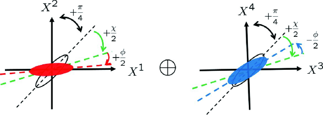
Figure 3: At $\theta=\pi$, the 4D uncertainty region for the $Sp(4;\mathbb{R})$ squeezed vacuum is exactly equal to the “direct sum” of the two 2D uncertainty regions described by two $Sp(2;\mathbb{R})$ squeezed vacua. The $Sp(4;\mathbb{R})$ squeezed vacuum thus realizes the squeezing in a 4D manner. The parameter $\rho$ denotes the degree of squeezing of both $Sp(2;\mathbb{R})$ squeezed vacua, $\chi$ stands for their overall rotation, and $\phi$ signifies the relative rotation between them. In particular at $(\chi,\phi)=(\frac{\pi}{2},0)$, both of the two squeezings are aligned to the “same” direction (the squeezing on $X^{1}-X^{2}$ plane is $X^{1}$ direction, and that on $X^{3}-X^{4}$ is $X^{3}$ direction), while at $(\chi,\phi)=(0,\frac{\pi}{2})$, two squeezings are “perpendicular” to each other (the squeezing on $X^{1}-X^{2}$ plane is $X^{1}$ direction, while that on $X^{3}-X^{4}$ plane is $X^{4}$ direction).

Since $\theta$ represents the squeezing parameter of the $Sp(4;\mathbb{R})$ squeeze operator, the case $(i)$ corresponds to the trivial vacuum and (237) is reduced to $\langle(\Delta{X^{m}})^{2}\rangle_{\text{sq}}=\frac{1}{4}$ (no sum for $m=1,2,3,4$), and so the case $(i)$ is rather trivial. Meanwhile for the case $(ii)$, at $(\chi,\phi)=(\frac{\pi}{2},0)$ or $(\chi,\phi)=(0,\frac{\pi}{2})$, the deviations (237) become

$$\langle(\Delta{X^{1}})^{2}\rangle_{\text{sq}}=\frac{1}{4}e^{2\rho},~{}~{}\langle(\Delta{X^{2}})^{2}\rangle_{\text{sq}}=\frac{1}{4}e^{-2\rho},~{}~{}\langle(\Delta{X^{3}})^{2}\rangle_{\text{sq}}=\frac{1}{4}e^{\pm 2\rho},~{}~{}\langle{(\Delta X^{4}})^{2}\rangle_{\text{sq}}=\frac{1}{4}e^{\mp 2\rho},$$ (240)

and non-trivially saturate the uncertainty bound:

$$\langle(\Delta{X^{1}})^{2}\rangle_{\text{sq}}~{}\langle(\Delta{X^{2}})^{2}\rangle_{\text{sq}}=\langle(\Delta{X^{3}})^{2}\rangle_{\text{sq}}~{}\langle(\Delta{X^{4}})^{2}\rangle_{\text{sq}}=\frac{1}{16}.$$ (241)

Performing similar calculations for the Schwinger-type squeezed vacuum, we obtain

$$\langle\!\langle(\Delta{X^{1/2}})^{2}\rangle\!\rangle_{\text{sq}}=\frac{1}{4}(\cosh\rho~{}+/-~{}\sinh\rho\sin(\chi+\phi))~{}~{}\geq~{}\frac{1}{16},$$ (242a)

$$\langle\!\langle(\Delta{X^{3/4}})^{2}\rangle\!\rangle_{\text{sq}}=\frac{1}{4}(\cosh\rho~{}+/-~{}\sinh\rho~{}\sin(\chi-\phi))~{}~{}\geq~{}\frac{1}{16},$$ (242b)

where (188) was used. Notice that the deviations do not depend on the parameter $\theta$ unlike the Dirac-type and are exactly equal to the Dirac-type at $\theta=\pi$ (239) with half squeezing. Therefore, (242) is identical to the uncertainty regions of two $Sp(2;\mathbb{R})$ squeezed vacua. This result is actually expected, since the Schwinger-type $Sp(4;\mathbb{R})$ squeezed vacuum (213) does not depend on $\theta$ and is simply the direct product of the two $Sp(2;\mathbb{R})$ squeezed vacua.

6 $Sp(4;\mathbb{R})$ squeezed coherent states

The $Sp(4;\mathbb{R})$ squeezed coherent state is introduced as the $Sp(4;\mathbb{R})$ squeezed vacuum displaced on 4D plane and exhibits a natural 4D generalization of the properties of the original $Sp(2;\mathbb{R})$ squeezed coherent state.

6.1 Squeezed coherent state

With the displacement operator $D_{a}(\alpha)=e^{\alpha a^{\dagger}-\alpha^{*}a}$, the two-mode and four-mode displacement operators are respectively given by

$$D(\alpha,\beta)=D_{a}(\alpha)D_{b}(\beta),~{}~{}~{}~{}~{}D(\alpha,\beta)=D_{a}(\alpha)D_{b}(\beta)D_{c}(\alpha)D_{d}(\beta).$$ (243)

It is straightforward to introduce a $Sp(4;\mathbb{R})$ version of the squeezed coherent state as

$$|\alpha,\beta,\text{sq}\rangle=D(\alpha,\beta)~{}S|0\rangle.$$ (244)

Each displacement operator acts to the two-mode $\hat{\psi}=(\hat{\psi}_{1}~{}\hat{\psi}_{2}~{}\hat{\psi}_{3}~{}\hat{\psi}_{4})^{t}=(a~{}a^{\dagger}~{}b~{}b^{\dagger})^{t}$ and the four-mode $\hat{\psi}=(\hat{\psi}_{1}~{}\hat{\psi}_{2}~{}\hat{\psi}_{3}~{}\hat{\psi}_{4})^{t}=(a~{}b^{\dagger}~{}c~{}d^{\dagger})^{t}$ as

$$D(\alpha,\beta)~{}\hat{\psi}~{}D(\alpha,\beta)^{\dagger}=\hat{\psi}-\varphi$$ (245)

where

$$\varphi=\begin{pmatrix}\tilde{\alpha}&\tilde{\alpha}^{*}&\tilde{\beta}&\tilde{\beta}^{*}\end{pmatrix}^{t}.$$ (246)

Relations

$$D~{}S~{}~{}\begin{pmatrix}\hat{\psi}_{1}\\ \hat{\psi}_{3}\end{pmatrix}~{}S^{\dagger}~{}D^{\dagger}~{}|\alpha,\beta,\text{sq}\rangle=\begin{pmatrix}0\\ 0\end{pmatrix},$$

$$D~{}S~{}~{}\begin{pmatrix}\hat{\psi}_{2}^{\dagger}\\ \hat{\psi}_{4}^{\dagger}\end{pmatrix}~{}S^{\dagger}~{}D^{\dagger}~{}|\alpha,\beta,\text{sq}\rangle=\begin{pmatrix}0\\ 0\end{pmatrix},$$ (247)

immediately tell that the squeezed coherent state satisfies the following operator eigenvalue equations

$$\hat{\psi}^{\prime}_{1}|\alpha,\beta,\text{sq}\rangle=\varphi^{\prime}_{1}|\alpha,\beta,\text{sq}\rangle,~{}~{}~{}~{}~{}~{}~{}~{}\hat{\psi}^{\prime}_{3}|\alpha,\beta,\text{sq}\rangle=\varphi^{\prime}_{3}|\alpha,\beta,\text{sq}\rangle,$$

$$(\hat{\psi}^{\prime}_{2})^{\dagger}|\alpha,\beta,\text{sq}\rangle={\varphi^{\prime}}^{*}_{2}|\alpha,\beta,\text{sq}\rangle,~{}~{}~{}(\hat{\psi}^{\prime}_{4})^{\dagger}|\alpha,\beta,\text{sq}\rangle={\varphi^{\prime}}^{*}_{4}|\alpha,\beta,\text{sq}\rangle,$$ (248)

where

$$\hat{\psi}^{\prime}\equiv S\hat{\psi}S^{\dagger}=M^{-1}\hat{\psi},~{}~{}~{}~{}\varphi^{\prime}\equiv M^{-1}\varphi.$$ (249)

For instance, the first equation of (248) for the two-mode Dirac-type squeezed coherent state reads as

$$\biggl{(}\cos\frac{\theta}{2}~{}a+i\sin\frac{\theta}{2}~{}\cosh\rho~{}e^{-i\phi}~{}b+\sin\frac{\theta}{2}~{}\sinh\rho~{}e^{-i\chi}~{}b^{\dagger}\biggr{)}|\alpha,\beta;\text{sq}\rangle$$

$$~{}~{}~{}~{}~{}~{}~{}~{}~{}~{}~{}~{}~{}~{}~{}~{}~{}~{}~{}~{}~{}~{}~{}~{}~{}~{}~{}=\biggl{(}\cos\frac{\theta}{2}~{}\alpha+i\sin\frac{\theta}{2}~{}\cosh\rho~{}e^{-i\phi}~{}\beta+\sin\frac{\theta}{2}~{}\sinh\rho~{}e^{-i\chi}~{}\beta^{*}\biggr{)}|\alpha,\beta;\text{sq}\rangle.$$ (250)

6.2 Several properties

• Two-mode $Sp(4;\mathbb{R})$ squeezed coherent state

For two-mode squeezed coherent state,

$$|\alpha,\beta,\text{sq}\rangle=D_{a}(\alpha)D_{b}(\beta)S~{}|0,0\rangle,$$ (251)

the expectation values of $X$s are derived as

$$\langle X^{1}\rangle_{(\alpha,\beta,\text{sq})}=\text{Re}(\alpha)=\langle X^{1}\rangle_{\alpha},~{}~{}~{}\langle X^{2}\rangle_{(\alpha,\beta,\text{sq})}=\text{Im}(\alpha)=\langle X^{2}\rangle_{\alpha},$$

$$\langle X^{3}\rangle_{(\alpha,\beta,\text{sq})}=\text{Re}(\beta)=\langle X^{3}\rangle_{\beta},~{}~{}~{}\langle X^{4}\rangle_{(\alpha,\beta,\text{sq})}=\text{Im}(\beta)=\langle X^{4}\rangle_{\beta}.$$ (252)

The expectation values (252) exactly coincide with those of the coherent states. Similarly, the deviations of $X$s are obtained as

$$\langle(\Delta X^{m})^{2}\rangle_{(\alpha,\beta,\text{sq})}=\langle(\Delta X^{m})^{2}\rangle_{(\alpha,\text{sq})}=\langle(X^{m})^{2}\rangle_{(\alpha,\text{sq})}-\langle X^{m}\rangle_{(\alpha,\text{sq})}^{2}=\langle(\Delta X^{m})^{2}\rangle_{\text{sq}}.~{}~{}~{}(\text{no sum for $m$}=1,2,3,4).$$ (253)

The deviations (253) are equal to those of the squeezed vacuum, (237) and (242). Thus, the position of the squeezed coherent state is accounted for by its coherent state part, while the deviation is by its squeezed state part, implying that the $Sp(4;\mathbb{R})$ squeezed coherent vacuum is the squeezed vacuum displaced by $(\alpha,\beta)$ on $\mathbb{C}^{2}\simeq\mathbb{R}^{4}$ plane. Obviously, this signifies a natural 4D generalization of the known properties of the original $Sp(2;\mathbb{R})$ squeezed coherent state [22].

• Four-mode $Sp(4;\mathbb{R})$ squeezed coherent state

From the four-mode generators of $Sp(4;\mathbb{R})$, we can define two kinds of annihilation operators :

$$A=X^{1}+iX^{2}=\frac{1}{\sqrt{2}}(a+b),~{}~{}B=X^{3}+iX^{4}=\frac{1}{\sqrt{2}}(c+d),$$ (254)

which satisfy $[A,A^{\dagger}]=[B,B^{\dagger}]=1.$ We construct the displacement operator as

$$D(\alpha,\beta)=D_{A}(\alpha)~{}D_{B}(\beta)=D_{a}(\frac{1}{\sqrt{2}}\alpha)~{}D_{b}(\frac{1}{\sqrt{2}}\alpha)~{}D_{c}(\frac{1}{\sqrt{2}}\beta)~{}D_{d}(\frac{1}{\sqrt{2}}\beta),$$ (255)

and introduce four-mode squeezed coherent state as

$$|\alpha,\beta,\text{sq}\rangle=D(\alpha,\beta)S|0,0,0,0\rangle.$$ (256)

It is easy to see that the expectation values of the coordinates are given by

$$\langle X^{1}\rangle_{(\alpha,\beta,\text{sq})}=\text{Re}(\alpha)=\langle X^{1}\rangle_{(\alpha,\beta)},~{}~{}~{}\langle X^{2}\rangle_{(\alpha,\beta,\text{sq})}=\text{Im}(\alpha)=\langle X^{2}\rangle_{(\alpha,\beta)},$$

$$\langle X^{3}\rangle_{(\alpha,\beta,\text{sq})}=\text{Re}(\beta)=\langle X^{3}\rangle_{(\alpha,\beta)},~{}~{}~{}\langle X^{4}\rangle_{(\alpha,\beta,\text{sq})}=\text{Im}(\beta)=\langle X^{4}\rangle_{(\alpha,\beta)},$$ (257)

and the deviations are

$$\langle(\Delta X^{m})^{2}\rangle_{(\alpha,\beta,\text{sq})}=\langle(X^{m})^{2}\rangle_{(\alpha,\beta,\text{sq})}-\langle X^{m}\rangle_{(\alpha,\beta,\text{sq})}^{2}=\langle(\Delta X^{m})^{2}\rangle_{\text{sq}}.~{}~{}~{}(\text{no sum for $m$}=1,2,3,4)$$ (258)

These results are equal to those of the two-mode case, (252) and (253). Hence, also for the four-mode, the $Sp(4;\mathbb{R})$ squeezed coherent vacuum is intuitively interpreted as the squeezed vacuum displaced by $(\alpha,\beta)$ on $\mathbb{C}^{2}\simeq\mathbb{R}^{4}$ plane.

7 Summary and discussions

We constructed the $Sp(4;\mathbb{R})$ squeezed coherent states and investigated their characteristic properties. We clarified the underlying hyperbolic geometry of the $Sp(2;\mathbb{R})$ squeezed states in the context of the 1st non-compact Hopf map. Taking advantage of the hierarchical geometry of the Hopf maps, we derived the $Sp(4;\mathbb{R})$ squeeze operator with Bloch four-hyperboloid geometry. Unlike the $Sp(2;\mathbb{R})$ case, the $Sp(4;\mathbb{R})$ squeezed vacua of the Dirac- and Schwinger-type are physically distinct. Based on the Euler angle decomposition of the $Sp(4;\mathbb{R})$ squeeze operator, we investigated the Schwinger-type $Sp(4;\mathbb{R})$ squeezed states, and clarified the physical meaning of the four coordinates of the Bloch four-hyperboloid. In particular, the entanglement concurrence of the $Sp(4;\mathbb{R})$ squeezed one-photon state was shown to be a geometric quantity determined by the 5th axis of the Bloch four-hyperboloid. We evaluated the mean values and deviations of the 4D non-commutative coordinates for the $Sp(4;\mathbb{R})$ squeezed (coherent) states and confirmed that they realize a natural 4D generalization of the original properties of the $Sp(2;\mathbb{R})$ squeezed states. The next direction will be a construction of an anharmonic oscillator Hamiltonian for the $Sp(4;\mathbb{R})$ squeezed state as in the $Sp(2;\mathbb{R})$ case [21] and its experimental realizations. Interestingly in [66], though not exactly same as the present case, Gerry and Benmoussa proposed analogous $SU(1,1)\otimes SU(1,1)$ entangled state of two squeezed states and suggested the possibility of generation in trapped ion experiments [67]. Their indication about experimental realization may also hold for the present state. Besides, the $SO(2,3)$ pseudo-spin coherent state accompanies the $SU(1,1)$ Berry phase as the $SU(1,1)$ pseudo-spin coherent state the $U(1)$ Berry phase. It is also interesting how such non-Abelian phase appears in optical experiments and brings pseudo-spin dynamics [68] particular to its non-Abelian nature, which may be compared to the exotic geometric phase of $SU(2)$ higher spins [69, 70].

The split quaternion was crucial in constructing the non-compact 2nd Hopf map. The split quaternion is closely related to the time-reversal operation for bosons by the following identification:

$$(q_{1},q_{2},q_{3})=(iT,T,i).$$ (259)

Here $T$ stands for the time-reversal operator for boson, $T^{2}=+1$, and $i$ is the imaginary unit. Since the time reversal operator is an anti-linear operator, $T$ is anticommutative with the imaginary unit, $Ti=-iT$, and so the identification $q_{1}=iT$ gives ${q_{1}}^{2}=+1$. Therefore, the triplet (259) can be regarded as a realization of the imaginary split quaternions, ${q_{1}}^{2}={q_{2}}^{2}=+1$, ${q_{3}}^{2}=-1$ and $q_{i}q_{j}=-q_{j}q_{i}$ $(i\neq j)$. In this way, the split quaternions naturally appear in the context of the time-reversal operation for bosons, just as the quaternions for fermions. More in detail as indicated in Table 1, there are intriguing correspondences between fermion and boson sectors starting from the quaternions and split quaternions.

	Quantum information	Quantum optics
Time-reversal symmetry	$T^{2}=-1$ (Fermion)	$T^{2}=+1$ (Boson)
Algebra	Quaternion $\mathbb{H}$	Split-quaternion $\mathbb{H}^{\prime}$
Bogoliubov trans.	$SO(2n)$	$Sp(2n;\mathbb{R})=U(n;\mathbb{H}^{\prime})$
Double covering group	$Spin(2n)$	$Mp(2n;\mathbb{R})$
Topological map	Hopf map	Non-compact Hopf map
Quantum manifold	Bloch sphere	Bloch hyperboloid
Fundamental quantum state	Qubit state	Squeezed state
Group coherent state	$SU(2)$ spin coherent state	$SU(1,1)$ pseudo-spin coherent state

Table 1: Comparison between quantum information sector of Bloch sphere and quantum optics sector of Bloch hyperboloid.

The list of the boson sector of Table 1 may suggest that the non-compact (hyperbolic) geometry is no less important than the compact (spherical) geometry for fermion sector already extensivley used in quantum information. As a concrete demonstration, we clarified the hyperbolic geometry of the squeezed states and applied it to construct a generalized $Sp(4;\mathbb{R})$ formulation of the squeezed states in the present work. It is very tempting to excavate further hyperbolic structure in quantum mechanics and quantum information theory. As a straightforward study along this line, one may think of applications of the non-compact 3rd Hopf map or more generally indefinite complex projective spaces. It should also be mentioned that the geometric structures of non-compact manifolds are richer than those of the compact counterparts: Non-compact manifolds generally accommodate compact manifolds as their submanifolds, which make the geometry of non-compact manifolds to be more interesting than that of compact manifolds. It is expected that the study of non-compact geometry will spur the developments of quantum information theory.

Though we focused on the squeezed states in this work, the non-compact Hopf map has begun to be applied in various fields, such as non-commutative geometry [47], twistorial quantum Hall effect [71], non-hermitian topological insulator [53, 72], and indefinite signature matrix model of string theory [73, 74, 75, 76]. Applications of the non-compact Hopf map may be ubiquitous. It may also be worthwhile to speculate its further possible applications.

Appendix A Symplectic algebra and metaplectic algebra

A.1 $U(n;\mathbb{H}^{\prime})$

We denote the split-quaternions as

$$q_{m}=\{q_{i},q_{4}\}=\{q_{1},q_{2},q_{3},1\},$$ (260)

which satisfy

$${q_{1}}^{2}={q_{2}}^{2}=-{q_{3}}^{2}=1,$$

$$q_{1}q_{2}=-q_{2}q_{1}=-q_{3},~{}~{}q_{3}q_{1}=-q_{1}q_{3}=-q_{2},~{}~{}q_{2}q_{3}=-q_{3}q_{2}=-q_{1}.$$ (261)

The quaternionic conjugate of $h=c^{m}~{}q_{m}$ $(c^{m}:\text{real parameters})$ is defined as

$$\bar{h}=\overline{(c^{m}~{}q_{m})}~{}\equiv~{}c^{m}~{}\bar{q}_{m},$$ (262)

with

$$\bar{q}_{m}=\{-q_{i},1\}.$$ (263)

$GL(n;\mathbb{H}^{\prime})$ is a group of split-quaternion valued $n\times n$ matrix

$$g=\begin{pmatrix}g_{11}&g_{12}&\cdots&g_{1n}\\ g_{21}&g_{22}&\cdots&g_{2n}\\ \vdots&\vdots&\ddots&\vdots\\ g_{n1}&g_{n2}&\cdots&g_{nn}\end{pmatrix}$$ (264)

where $g_{ij}$ are given by

$$g_{ij}=c_{ij}^{m}~{}q_{m}$$ (265)

with $c_{ij}^{m}$ real numbers. The (split-)quaternionic Hermitian conjugate of $g$ is defined as

$$g^{\ddagger}\equiv(\bar{g})^{t}=\begin{pmatrix}\overline{g_{11}}&\overline{g_{21}}&\cdots&\overline{g_{n1}}\\ \overline{g_{12}}&\overline{g_{22}}&\cdots&\overline{g_{n2}}\\ \vdots&\vdots&\ddots&\vdots\\ \overline{g_{1n}}&\overline{g_{2n}}&\cdots&\overline{g_{nn}}\end{pmatrix},$$ (266)

where $\overline{q_{ij}}=c_{ij}^{m}\bar{q}_{m}$. The quaternionic conjugate and the quaternionic Hermitian conjugate have the following properties:

$$\overline{(h_{1}~{}h_{2})}=\overline{h_{2}}~{}\overline{h_{1}},$$ (267a)

$$(g_{1}\cdot g_{2})^{\ddagger}={g_{2}}^{\ddagger}\cdot{g_{1}}^{\ddagger}.$$ (267b)

Here, we consider the $GL(n;\mathbb{H}^{\prime})$ transformation that keeps the inner product of split-quaternion vectors invariant,

$$g^{\ddagger}~{}g=1,$$ (268)

and such a transformation is called the split-quaternionic unitary transformation denoted by $U(n;\mathbb{H}^{\prime})$. When we introduce $u(n;\mathbb{H}^{\prime})$ generator $X$ as

$$g=e^{X},$$ (270)

(268) imposes the following condition on $X$:

$$X^{\ddagger}=-X.$$ (271)

The generators of $U(n;\mathbb{H}^{\prime})$ are simply split-quaternionic anti-Hermitian matrices. Then, the $u(n;\mathbb{H}^{\prime})$ basis matrices are given by

$$\begin{pmatrix}0&0&0&0&0\\ 0&0&\ddots&0&0\\ 0&0&q_{i}&0&0\\ 0&\ddots&0&0&0\\ 0&0&0&0&0\end{pmatrix},~{}~{}~{}\begin{pmatrix}0&0&0&0&0\\ 0&\ddots&0&q_{m}&0\\ 0&0&0&0&0\\ 0&-\bar{q}_{m}&0&\ddots&0\\ 0&0&0&0&0\end{pmatrix}.$$ (272)

The dimension of $u(n;\mathbb{H}^{\prime})$ algebra is then counted as

$$\dim U(n;\mathbb{H}^{\prime})=n\times 3+\frac{n(n-1)}{2}\times 4=n(2n+1).$$ (273)

We can realize the split-quaternions by the $su(1,1)$ matrices

$$\{q_{1},q_{2},q_{3},1\}=\{\sigma_{x},\sigma_{z},i\sigma_{y},1_{2}\}$$ (274)

and demonstrate the isomorphism $U(n;\mathbb{H}^{\prime})\simeq Sp(2n;\mathbb{R})$ as follows. Notice that the matrices on the right-hand side of (274) are all real matrices, and so the $U(n;\mathbb{H}^{\prime})$ group elements can be expressed by real matrices, $g^{*}=g$. In the matrix realization, the split-quaternionic conjugate is not equal to the usual Hermitian conjugate but given by

$$\bar{q}_{m}=\{-\sigma_{x},-\sigma_{z},-i\sigma_{y},1_{2}\}=\epsilon^{t}~{}{q_{m}}^{\dagger}~{}\epsilon=\epsilon^{t}~{}{q_{m}}^{t}~{}\epsilon$$ (275)

where

$$\epsilon\equiv i\sigma_{y}.$$ (276)

Consequently for the matrix realization of $U(n;\mathbb{H}^{\prime})$, we have

$$g^{\ddagger}=\mathcal{E}^{t}~{}g^{t}~{}\mathcal{E},$$ (277)

with

$$\mathcal{E}=\begin{pmatrix}\epsilon&0&0&0\\ 0&\epsilon&0&0\\ 0&0&\ddots&0\\ 0&0&0&\epsilon\end{pmatrix}.$$ (278)

The $U(n;\mathbb{H}^{\prime})$ condition (268) can be expressed as

$$g^{t}~{}\mathcal{E}~{}g=\mathcal{E}.$$ (279)

Under the following unitary transformation

$$g~{}~{}\rightarrow~{}~{}U~{}g~{}U^{t}$$ (280)

where

$$U=\begin{pmatrix}\boldsymbol{e}_{1}&\boldsymbol{e}_{3}&\cdots&\boldsymbol{e}_{2n-1}&\boldsymbol{e}_{2}&\boldsymbol{e}_{4}&\cdots&\boldsymbol{e}_{2n}\end{pmatrix}$$ (281)

with $(\boldsymbol{e}_{a})_{b}\equiv\delta_{ab}$ $(a,b=1,2,\cdots,2n)$, (279) is transformed as

$$g^{t}~{}J~{}g=J.$$ (282)

This is the very condition that defines the $Sp(2n;\mathbb{R})$ group (286). We thus find

$$U(n;\mathbb{H}^{\prime})\simeq Sp(2n;\mathbb{R}).$$ (283)

A.2 Symplectic algebra $sp(2n;\mathbb{R})$

Elements of the $Sp(2n;\mathbb{R})$ group are given by a real matrix $g$ that satisfies the condition

$$g^{t}~{}J~{}g=J,$$ (286)

where $J$ is called the $Sp(2n;\mathbb{R})$ invariant matrix:

$$J=\begin{pmatrix}0&1_{n}\\ -1_{n}&0\end{pmatrix}.$$ (287)

With the generator $X$

$$g=e^{X},$$ (288)

the relation (286) can be rewritten as

$$X^{t}J+JX=0,$$ (289)

or equivalently

$$(JX)^{t}=JX.$$ (290)

(290) determines the form of $X$ as

$$X=\begin{pmatrix}M&S_{1}\\ S_{2}&-M^{t}\end{pmatrix},$$ (291)

where $M$ denotes arbitrary $n\times n$ real matrix, and $S_{1}$ and $S_{2}$ are two arbitrary $n\times n$ symmetric real matrices. The dimension of the symplectic algebra is readily obtained as

$$\dim(sp(2n;\mathbb{R}))=(\text{real degrees of }M)+(\text{real degrees of }S)=n^{2}+\frac{n(n+1)}{2}\times 2=n(2n+1).$$ (292)

From (291), we can choose $n(2n+1)$ $sp(2n;\mathbb{R})$ basis matrices as

$$(X^{i}_{j})_{ab}=\delta_{a,i}\delta_{b,j}-\delta_{n+i,b}\delta_{n+j,a}=(X^{j}_{i})_{ba},$$

$$(X^{ij})_{ab}=\delta_{a,i}\delta_{b,n+j}+\delta_{a,j}\delta_{b,n+j}=(X^{ji})_{ab},$$

$$(X_{ij})_{ab}=-\delta_{a,n+i}\delta_{b,j}-\delta_{a,n+j}\delta_{b,j}=(X_{ji})_{ab},$$ (293)

where $i,j=1,2,\cdots,n$ and $a,b=1,2,\cdots,2n$. They satisfy

$$[X_{ij},X_{kl}]=[X^{ij},X^{kl}]=0,$$

$$[X_{ij},X^{kl}]=X_{i}^{l}\delta_{j}^{k}+X_{j}^{l}\delta_{i}^{k}+X_{i}^{k}\delta_{j}^{l}+X_{j}^{k}\delta_{i}^{l},$$

$$[X_{ij},X_{k}^{l}]=X_{ik}\delta_{j}^{l}+X_{jk}\delta_{i}^{l},$$

$$[X^{ij},X^{l}_{k}]=-X^{il}\delta_{k}^{j}-X^{jl}\delta_{k}^{i},$$

$$[X_{j}^{i},X_{k}^{l}]=X^{i}_{k}\delta_{j}^{l}-X_{j}^{l}\delta_{k}^{i}.$$ (294)

The $Sp(2n,\mathbb{R})$ invariant matrix (287) is diagonalized by the following unitary transformation

$$\Omega~{}J~{}\Omega^{\dagger}=iK,$$ (295)

where $K$ is a diagonal matrix with neutral components:

$$K\equiv\begin{pmatrix}1_{n}&0_{n}\\ 0_{n}&-1_{n}\end{pmatrix},~{}~{}~{}~{}~{}~{}~{}(K^{-1}=K^{\dagger}=K)$$ (296)

and $\Omega$ can be taken as

$$\Omega=\frac{1}{\sqrt{2}}\begin{pmatrix}R&-iR\\ R&iR\end{pmatrix}~{}~{}~{}~{}~{}~{}~{}~{}~{}~{}(\Omega^{\dagger}=\Omega^{-1})$$ (297)

with $n\times n$ matrix $R$

$$R=\begin{pmatrix}0&0&0&\cdots&0&1\\ 0&0&0&\cdots&1&0\\ 0&0&0&1&0&0\\ 0&0&1&\cdots&0&0\\ 0&1&0&\cdots&0&0\\ 1&0&0&\cdots&0&0\end{pmatrix}.$$ (298)

The $Sp(2n;\mathbb{R})$ group condition (286) can be expressed as

$$g^{t}\Omega^{\dagger}~{}K~{}\Omega g=\Omega^{\dagger}~{}K~{}\Omega.$$ (299)

Since $g$ is a real matrix, $g^{t}=g^{\dagger}$, (299) is rewritten as

$$(\Omega~{}g~{}\Omega^{\dagger})^{\dagger}~{}K~{}(\Omega~{}g~{}\Omega^{\dagger})=K.$$ (300)

Therefore,

$$g^{\prime}\equiv\Omega~{}g~{}\Omega^{\dagger}$$ (301)

realizes another representation of the $Sp(2n,\mathbb{R})$ group element that satisfies

$${g^{\prime}}^{\dagger}~{}K~{}g^{\prime}=K.$$ (302)

Notice that $g^{\prime}$ no longer denotes a real matrix unlike $g$. Since $g$ is a $2n\times 2n$ real matrix, $g^{\prime}$ (301) with $\Omega$ (297) is parameterized as

$$g^{\prime}=\begin{pmatrix}U&V^{*}\\ V&U^{*}\end{pmatrix},$$ (303)

where each of $U$ and $V$ is a $n\times n$ complex matrix. For $g^{\prime}$ subject to (302), the blocks $U$ and $V$ must satisfy

$$U^{\dagger}U-V^{\dagger}V=1_{n},~{}~{}~{}~{}~{}~{}U^{t}V-V^{t}U=0_{n}.$$ (304)

The (real) number of constraints of (304) is $(n^{2})+(n^{2}-n)=n(2n-1)$, and then the real degrees of freedom $g^{\prime}$ is obtained as

$$(2n)^{2}-n(2n-1)=n(2n+1),$$ (305)

which is indeed the dimension of the $sp(2n;\mathbb{R})$ algebra (292). We can readily identify the form of the associated $sp(2n;\mathbb{R})$ generator $X^{\prime}$

$$\begin{pmatrix}U&V^{*}\\ V&U^{*}\end{pmatrix}=e^{iX^{\prime}}$$ (306)

as

$$X^{\prime}=\begin{pmatrix}H&S^{*}\\ -S&-H^{*}\end{pmatrix},$$ (310)

where $H$ is arbitrary $n\times n$ Hermitian matrix and $S$ is arbitrary $n\times n$ symmetric complex matrix. Obviously, the maximal Cartan sub-algebra is given by

$$\begin{pmatrix}H&0\\ 0&-H^{*}\end{pmatrix},$$ (311)

which is the generator of $U(n)$. ($-H^{*}$ denotes the complex representation of $H$ and satisfies the same algebra of $H$.) $U(n)$ is the maximal Cartan group of the Cartan-Iwasawa decomposition of $Sp(2n;\mathbb{R})$ (see (21)). (302) imposes the following condition on $X^{\prime}$:

$$X^{\prime\dagger}K-KX^{\prime}=0$$ (312)

or

$$X^{\prime\dagger}=KX^{\prime}K,$$ (313)

and so the block matrices of $X$ must satisfy

$$H^{\dagger}=H,~{}~{}~{}S^{t}=S.$$ (314)

$H$ is a $n\times n$ Hermitian matrix and $S$ a complex symmetric matrix. Notice that

$$KX^{\prime}=\begin{pmatrix}H&S^{*}\\ S&H^{*}\end{pmatrix}$$ (315)

denotes a Hermitian matrix. By sandwitching $KX$ by a Dirac spinor operator

$$\hat{\psi}=\begin{pmatrix}a_{1}&\cdots&a_{n}&b_{1}^{\dagger}&\cdots&b_{N}^{\dagger}\end{pmatrix}^{t}$$ (316)

and its conjugate, we can construct Hermitian operators that satisfy $sp(2n;\mathbb{R})$ algebra. From the Hermitian operators, independent operators are extracted as

$$X_{i}^{j}=\frac{1}{2}\{a_{i},a_{j}^{\dagger}\}+\frac{1}{2}\{b_{i},b_{j}^{\dagger}\}={X_{j}^{i}}^{\dagger}~{}~{}:~{}~{}n^{2},$$ (317a)

$$X^{ij}=a_{i}^{\dagger}b_{j}^{\dagger}+a_{j}^{\dagger}b_{i}^{\dagger}=X^{ji}~{}~{}~{}~{}~{}~{}~{}~{}~{}~{}~{}~{}~{}~{}~{}:~{}~{}\frac{1}{2}n(n+1),$$ (317b)

$$X_{ij}=a_{i}b_{j}+a_{j}b_{i}=X_{ji}~{}~{}~{}~{}~{}~{}~{}~{}~{}~{}~{}~{}~{}~{}~{}~{}:~{}~{}\frac{1}{2}n(n+1).$$ (317c)

They indeed constitute non-Hermitian operators for the $sp(2n;\mathbb{R})$ algebra (294). In particular

$$X_{i}^{j}=a_{j}^{\dagger}a_{i}+b_{j}^{\dagger}b_{i}+\delta_{i}^{j}$$ (318)

satisfy the maximal Cartan $u(n)$ sub-algebra. The $Sp(2n;\mathbb{R})$ Casimir is derived as

$$C=X^{ij}X_{ij}+X_{ij}X^{ij}-2X^{i}_{j}X^{j}_{i}=-2(a_{i}^{\dagger}a_{i}-b^{\dagger}b_{i}+n)(a_{i}^{\dagger}a_{i}-b_{i}^{\dagger}b_{i}-n).$$ (319)

A.3 Metaplectic algebra

The metaplectic group $Mp(2n;\mathbb{R})$ is the double cover of the symplectic group $Sp(2n;\mathbb{R})$:

$$Mp(2n;\mathbb{R})/\mathbb{Z}_{2}\simeq Sp(2n;\mathbb{R}).$$ (320)

Instead of the “complex” operator $\hat{\psi}$ (316), we here introduce a “real” operator

$$\hat{\phi}=\begin{pmatrix}a_{1}&\cdots&a_{n}&a_{1}^{\dagger}&\cdots&a_{n}^{\dagger}\end{pmatrix}^{t},$$ (321)

that satisfies the real condition

$$\hat{\phi}^{*}=C\hat{\phi}~{}~{}~{}~{}~{}(C\equiv\begin{pmatrix}0&1_{n}\\ 1_{n}&0\end{pmatrix})$$ (322)

and

$$[\hat{\phi}_{\alpha},\hat{\phi}_{\beta}]=J_{\alpha\beta}$$ (323)

with $J$ (287). From (321), we can construct the following Hermitian operator

$$O_{M}=\frac{1}{2}~{}\hat{\phi}^{t}~{}CKX~{}\hat{\phi}=-\frac{1}{2}~{}\hat{\phi}^{t}~{}JX~{}\hat{\phi}.$$ (324)

Here $X$ is given by (310) and $JX$ is

$$J~{}X=-\begin{pmatrix}S&H^{*}\\ H&S^{*}\end{pmatrix}=(JX)^{t}.$$ (325)

From the original $sp(2n;\mathbb{R})$ matrix $X$ (291), we can also construct a symmetric matrix

$$JX=\begin{pmatrix}S_{2}&-M^{t}\\ -M&-S_{1}\end{pmatrix}=(JX)^{t}$$ (326)

and associated non-Hermitian operator

$$\hat{X}=-\frac{1}{2}~{}\hat{\phi}^{t}~{}JX~{}\hat{\phi}.$$ (327)

The basis matrices of (326) are given by

$$(JX^{i}_{j})_{a,b}=(JX^{i}_{j})_{b,a}=-\delta_{a,n+i}\delta_{b,j}-\delta_{a,j}\delta_{b,n+i},$$

$$(JX^{ij})_{a,b}=(JX^{ji})_{a,b}=-\delta_{a,n+i}\delta_{b,n+j}-\delta_{a,n+j}\delta_{b,n+i},$$

$$(JX_{ij})_{a,b}=(JX_{ji})_{a,b}=\delta_{a,i}\delta_{b,j}+\delta_{a,j}\delta_{b,i},~{}~{}~{}~{}~{}~{}~{}~{}~{}~{}(a,b=1,2,\cdots,2n)$$ (328)

where $X$s are (293). It is not difficult to verify that the corresponding operators satisfy the $sp(2n;\mathbb{R})$ algebra (294) using the relations, $J^{2}=-1_{2n}$ and $(JX)^{t}=JX$. The basis operators corresponding to (328) are obtained as

$$\hat{X}_{j}^{i}=\frac{1}{2}\{a^{\dagger}_{i},a_{j}\}=a^{\dagger}_{i}a_{j}+\frac{1}{2}\delta_{ij}=(\hat{X}_{i}^{j})^{\dagger},~{}~{}~{}~{}:~{}n^{2},$$

$$\hat{X}^{ij}=a_{i}^{\dagger}a_{j}^{\dagger}=\frac{1}{2}\{a_{i}^{\dagger},a_{j}^{\dagger}\}=\hat{X}^{ji},~{}~{}~{}~{}~{}~{}~{}~{}~{}~{}~{}~{}~{}~{}~{}:~{}\frac{1}{2}n(n+1)$$

$$\hat{X}_{ij}=a_{i}a_{j}=\frac{1}{2}\{a_{i},a_{j}\}=\hat{X}_{ji},~{}~{}~{}~{}~{}~{}~{}~{}~{}~{}~{}~{}~{}~{}~{}~{}:~{}\frac{1}{2}n(n+1)$$ (329)

which satisfy (294). These operators for metaplectic representation can also be obtained from (317) with replacement of the operator $b$ by $a$ and by changing the overall scale factor by $1/2$.

The $Sp(2n;\mathbb{R})$ Casimir operator for the metaplectic representation becomes a constant:

$$C=\hat{X}^{ij}\hat{X}_{ij}+\hat{X}_{ij}\hat{X}^{ij}-2\hat{X}^{i}_{j}\hat{X}^{j}_{i}=n(n+\frac{1}{2}).$$ (330)

A.4 Bogoliubov canonical transformations

We consider the canonical commutation relations for $n$ bosons:

$$[a_{i},a_{j}^{\dagger}]=\delta_{ij},~{}~{}~{}[a_{i},a_{j}]=0.~{}~{}~{}~{}~{}(i,j=1,2,\cdots,n)$$ (331)

The transformation preserving the canonical commutation relations is called the Bogoliubov canonical transformation. Let us consider a general linear transformation of the bosonic operators:

$$a^{\prime}_{i}=u_{ji}a_{j}+v_{ji}a^{\dagger}_{j}.$$ (332)

For the canonical transformation, $u_{ij}$ and $v_{ij}$ should satisfy

$$[a^{\prime}_{i},{a^{\prime}}_{j}^{\dagger}]=\delta_{ij},~{}~{}[a^{\prime}_{i},a^{\prime}_{j}]=0~{}~{}~{}\rightarrow~{}~{}~{}u_{ki}u_{jk}^{*}-v_{ki}v_{kj}^{*}=\delta_{ij},~{}~{}u_{ki}v_{kj}-v_{ki}u_{kj}=0,$$ (333)

which, in matrix notation, becomes

$$U^{t}U^{*}-V^{t}V^{*}=1_{n},~{}~{}~{}~{}U^{t}V-V^{t}U=0_{n}.$$ (334)

(334) is nothing but the condition used in the definition of the $Sp(2n;\mathbb{R})$ group (304). We thus find that the canonical transformation for bosons is described by the symplectic group [13, 15].

In a similar manner, we can readily identify the canonical transformation group for fermions. The commutation relations for $n$ fermions are given by

$$\{f_{i},f_{j}^{\dagger}\}=\delta_{ij},~{}~{}~{}\{f_{i},f_{j}\}=0.~{}~{}~{}~{}~{}(i,j=1,2,\cdots,n)$$ (335)

Among general linear transformations

$$f^{\prime}_{i}=u_{ji}f_{j}+v_{ji}f^{\dagger}_{j},$$ (336)

the canonical transformation is realized as

$$\{f_{i},{f^{\prime}}_{j}^{\dagger}\}=\delta_{ij},~{}~{}\{f^{\prime}_{i},f^{\prime}_{j}\}=0~{}~{}\rightarrow~{}~{}~{}u_{ki}u_{jk}^{*}+v_{ki}v_{kj}^{*}=\delta_{ij},~{}~{}u_{ki}v_{kj}+v_{ki}u_{kj}=0,$$ (337)

which, in matrix notation, is given by

$$U^{t}U^{*}+V^{t}V^{*}=1_{n},~{}~{}U^{t}V+V^{t}U=0_{n}.$$ (338)

Recall that the arbitrary $2n\times 2n$ real matrix $g$ is unitarily equivalent to $g^{\prime}=\Omega~{}g~{}\Omega^{\dagger}=\begin{pmatrix}U&V^{*}\\ V&U^{*}\end{pmatrix}$ (303). Therefore, the condition for the $SO(2n)$ group element $g$,

$$g^{t}g=1_{2n},$$ (339)

can be restated for $g^{\prime}$ as

$$g^{\prime\dagger}g^{\prime}=1_{2n}.$$ (340)

(340) imposes the following conditions on the block components of $g^{\prime}$ as

$$U^{\dagger}U+V^{\dagger}V=1_{n},~{}~{}~{}U^{t}V+V^{t}U=0_{n},$$ (341)

which is exactly the condition (338), so we find that the canonical transformation for $n$ fermions is the $SO(2n)$ transformation [14, 15]. For comparison to the expression of the $sp(2n;\mathbb{R})$ generator (310), we derive the matrix form of the $so(2n)$ generator $X^{\prime}$ defined by $g^{\prime}=e^{iX^{\prime}}$. (340) implies

$$X^{\prime\dagger}=X^{\prime},$$ (342)

or

$$X^{\prime}=\begin{pmatrix}H&A^{*}\\ -A&-H^{*}\end{pmatrix}.$$ (343)

Here, $H$ and $A$ respectively denote arbitrary $n\times n$ Hermitian matrix and complex anti-symmetric matrix with $n^{2}$ and $n(n-1)$ real degrees of freedom. In total, $X^{\prime}$ carries $n(2n-1)$ real degrees of freedom, $i.e.$, the dimension of the $so(2n)$ algebra.

Appendix B Useful formulas for the split-quaternions and $so(2,3)$ algebra

B.1 Algebra of split-quaternions

The algebra of the split-quaternions (261) is concisely expressed as

$$\{q^{i},q^{j}\}=-2g^{ij},~{}~{}~{}[q^{i},q^{j}]=-2\epsilon^{ijk}q_{k},$$ (344)

where

$$g_{ij}=g^{ij}=\text{diag}(-1,-1,+1),~{}~{}~{}\epsilon^{123}=1.$$ (345)

The split quaternions satisfy

$$q^{m}\bar{q}^{n}+q^{n}\bar{q}^{m}=\bar{q}^{m}q^{n}+\bar{q}^{n}q^{m}=2g^{mn},$$ (346a)

$$q^{m}\bar{q}^{n}-q^{n}\bar{q}^{m}=2{\eta}^{mni}q_{i},~{}~{}~{}~{}~{}\bar{q}^{m}q^{n}-\bar{q}^{n}q^{m}=2\bar{\eta}^{mni}q_{i}$$ (346b)

and

$$q^{i}q^{m}=-{\eta}^{mni}q_{n},~{}~{}~{}~{}q^{m}q^{i}=\bar{\eta}^{mni}q_{n},$$ (347a)

$$q^{i}\bar{q}^{m}=-\bar{\eta}^{mni}\bar{q}_{n},~{}~{}~{}~{}\bar{q}^{m}q^{i}=\eta^{mni}\bar{q}_{n}.$$ (347b)

Here, $g_{mn}$ is

$$g_{mn}=\text{diag}(-1,-1,+1,+1),$$ (348)

and $\eta^{mni}$ and $\bar{\eta}^{mni}$ are the ’t Hooft symbols:

$$\eta^{mni}=\epsilon^{mni4}+g^{mi}g^{n4}-g^{ni}g^{m4},~{}~{}~{}\bar{\eta}^{mni}=\epsilon^{mni4}-g^{mi}g^{n4}+g^{ni}g^{m4}.$$ (349)

They satisfy

$$\frac{1}{2}\epsilon_{mnpq}\eta^{pqi}=\eta_{mn}^{~{}~{}~{}i},~{}~{}~{}~{}\frac{1}{2}\epsilon_{mnpq}\bar{\eta}^{pqi}=-\bar{\eta}_{mn}^{~{}~{}~{}i},$$ (350a)

$$\eta^{mni}\eta_{mnj}=4\delta^{i}_{~{}j},~{}~{}~{}~{}~{}~{}~{}\bar{\eta}^{mni}\bar{\eta}_{mnj}=4\delta^{i}_{~{}j}~{}~{}~{}~{}~{}~{}~{}~{}\eta^{mni}\bar{\eta}_{mnj}=0.$$ (350b)

B.2 $so(2,3)$ generators and other variants

Using the split-quaternions, we can realize the $SO(2,3)$ gamma matrices as

$$\gamma^{m}=\begin{pmatrix}0&\bar{q}^{m}\\ q^{m}&0\end{pmatrix},~{}~{}~{}\gamma^{5}=\begin{pmatrix}1&0\\ 0&-1\end{pmatrix},$$ (351)

which satisfy

$$\{\gamma^{a},\gamma^{b}\}=2g^{ab}$$ (352)

with

$$g_{ab}=g^{ab}=\text{diag}(-1,-1,+1,+1,+1).$$ (353)

The $so(2,3)$ generators, $\sigma^{ab}=-i\frac{1}{4}[\gamma^{a},\gamma^{b}]$, are obtained as

$$\sigma^{mn}=-i\frac{1}{4}[\gamma^{m},\gamma^{n}]=-i\frac{1}{2}\begin{pmatrix}\bar{\eta}^{mni}q_{i}&0\\ 0&{\eta}^{mni}q_{i}\end{pmatrix},~{}~{}~{}~{}\sigma^{m5}=-\sigma^{5m}=-i\frac{1}{4}[\gamma^{m},\gamma^{5}]=i\frac{1}{2}\begin{pmatrix}0&\bar{q}^{m}\\ -q^{m}&0\end{pmatrix},$$ (354)

and they satisfy

$$[\sigma_{ab},\sigma_{cd}]=i(g_{ac}\sigma_{bd}-g_{ad}\sigma_{cd}+g_{bd}\sigma_{ac}-g_{cd}\sigma_{ad}).$$ (355)

As maximal sub-algebra, the $so(2,3)$ algebra accommodates $so(2,2)\simeq su(1,1)\oplus su(1,1)$ whose matrix representation is given by

$${S}^{i}\equiv-\frac{1}{4}{\eta}_{mn}^{~{}~{}i}\sigma^{mn}=i\frac{1}{2}\begin{pmatrix}0&0\\ 0&q^{i}\end{pmatrix},~{}~{}~{}\bar{S}^{i}\equiv-\frac{1}{4}\bar{\eta}_{mn}^{~{}~{}i}\sigma^{mn}=i\frac{1}{2}\begin{pmatrix}q^{i}&0\\ 0&0\end{pmatrix}.$$ (356)

They satisfy

$$[S^{i},S^{j}]=-i\epsilon^{ijk}S_{k},~{}~{}~{}[\bar{S}^{i},\bar{S}^{j}]=-i\epsilon^{ijk}\bar{S}_{k},~{}~{}~{}[S^{i},\bar{S}^{j}]=0.$$ (357)

The remaining algebraic relations of $so(2,3)$ are

$$[S^{i},\sigma^{m5}]=-i\frac{1}{2}\eta^{mni}\sigma_{n5},~{}~{}~{}[\bar{S}^{i},\sigma^{m5}]=-i\frac{1}{2}\bar{\eta}^{mni}\sigma_{n5}.$$ (358)

As in the main text, we express the split-quaternions as (39)

$$\{q^{1},q^{2},q^{3},q^{4}\}=\{\sigma_{x},\sigma_{y},-i\sigma_{z},1_{2}\},$$ (359)

and the $SO(2,3)$ gamma matrices become

$$\gamma^{1}=\begin{pmatrix}0&-\sigma_{x}\\ \sigma_{x}&0\end{pmatrix},~{}~{}\gamma^{2}=\begin{pmatrix}0&-\sigma_{y}\\ \sigma_{y}&0\end{pmatrix},~{}~{}\gamma^{3}=\begin{pmatrix}0&i\sigma_{z}\\ -i\sigma_{z}&0\end{pmatrix},~{}~{}\gamma^{4}=\begin{pmatrix}0&1_{2}\\ 1_{2}&0\end{pmatrix},~{}~{}\gamma^{5}=\begin{pmatrix}1_{2}&0\\ 0&-1_{2}\end{pmatrix}.$$ (360)

The $so(2,3)$ matrices are

$$\!\!\!\!\!\!\!\!\!\!\sigma^{12}=-\frac{1}{2}\begin{pmatrix}\sigma_{z}&0\\ 0&\sigma_{z}\end{pmatrix},~{}~{}~{}\sigma^{13}=-i\frac{1}{2}\begin{pmatrix}\sigma_{y}&0\\ 0&\sigma_{y}\end{pmatrix},~{}~{}~{}\sigma^{14}=i\frac{1}{2}\begin{pmatrix}\sigma_{x}&0\\ 0&-\sigma_{x}\end{pmatrix},~{}~{}~{}\sigma^{15}=-i\frac{1}{2}\begin{pmatrix}0&\sigma_{x}\\ \sigma_{x}&0\end{pmatrix},~{}~{}~{}\sigma^{23}=i\frac{1}{2}\begin{pmatrix}\sigma_{x}&0\\ 0&\sigma_{x}\end{pmatrix},$$

$$\!\!\!\!\!\!\!\!\!\!\sigma^{24}=i\frac{1}{2}\begin{pmatrix}\sigma_{y}&0\\ 0&-\sigma_{y}\end{pmatrix},~{}~{}~{}\sigma^{25}=-i\frac{1}{2}\begin{pmatrix}0&\sigma_{y}\\ \sigma_{y}&0\end{pmatrix},~{}~{}~{}\sigma^{34}=\frac{1}{2}\begin{pmatrix}\sigma_{z}&0\\ 0&-\sigma_{z}\end{pmatrix},~{}~{}~{}\sigma^{35}=-\frac{1}{2}\begin{pmatrix}0&\sigma_{z}\\ \sigma_{z}&0\end{pmatrix},~{}~{}~{}\sigma^{45}=i\frac{1}{2}\begin{pmatrix}0&1\\ -1&0\end{pmatrix}.$$ (361)

They satisfy

$$(\gamma^{a})^{\dagger}=\gamma_{a},~{}~{}~{}~{}~{}(\sigma^{ab})^{\dagger}=\sigma_{ab}.$$ (362)

The associated Hermitian matrices $k^{a}$ and $k^{ab}$ (129) are represented as

$$k^{i}=\begin{pmatrix}0&i\kappa^{i}\\ -i\kappa^{i}&0\end{pmatrix},~{}~{}k^{4}=\begin{pmatrix}0&\sigma_{z}\\ \sigma_{z}&0\end{pmatrix},~{}~{}k^{5}=\begin{pmatrix}\sigma_{z}&0\\ 0&-\sigma_{z}\end{pmatrix},$$ (363)

and

$$k^{mn}=-\frac{1}{2}\begin{pmatrix}\bar{\eta}^{mni}\kappa_{i}&0\\ 0&{\eta}^{mni}\kappa_{i}\end{pmatrix},~{}~{}k^{i5}=-\frac{1}{2}\begin{pmatrix}0&\kappa^{i}\\ \kappa^{i}&0\end{pmatrix},~{}~{}k^{45}=i\frac{1}{2}\begin{pmatrix}0&\sigma_{z}\\ -\sigma_{z}&0\end{pmatrix}.$$ (364)

With the Pauli matrices, they are given by

$$k^{x}=\begin{pmatrix}0&-i\sigma_{y}\\ i\sigma_{y}&0\end{pmatrix},~{}~{}k^{y}=\begin{pmatrix}0&i\sigma_{x}\\ -i\sigma_{x}&0\end{pmatrix},~{}~{}k^{z}=\begin{pmatrix}0&i1_{2}\\ -i1_{2}&0\end{pmatrix},~{}~{}k^{4}=\begin{pmatrix}0&\sigma_{z}\\ \sigma_{z}&0\end{pmatrix},~{}~{}k^{5}=\begin{pmatrix}\sigma_{z}&0\\ 0&-\sigma_{z}\end{pmatrix}$$ (365)

and

$$k^{12}=-\frac{1}{2}\begin{pmatrix}1_{2}&0\\ 0&1_{2}\end{pmatrix},~{}~{}k^{13}=-\frac{1}{2}\begin{pmatrix}\sigma_{x}&0\\ 0&\sigma_{x}\end{pmatrix},~{}~{}k^{14}=\frac{1}{2}\begin{pmatrix}-\sigma_{y}&0\\ 0&\sigma_{y}\end{pmatrix},~{}~{}k^{15}=\frac{1}{2}\begin{pmatrix}0&\sigma_{y}\\ \sigma_{y}&0\end{pmatrix},~{}~{}k^{23}=-\frac{1}{2}\begin{pmatrix}\sigma_{y}&0\\ 0&\sigma_{y}\end{pmatrix},$$

$$k^{24}=\frac{1}{2}\begin{pmatrix}\sigma_{x}&0\\ 0&-\sigma_{x}\end{pmatrix},~{}~{}k^{25}=-\frac{1}{2}\begin{pmatrix}0&\sigma_{x}\\ \sigma_{x}&0\end{pmatrix},~{}~{}k^{34}=\frac{1}{2}\begin{pmatrix}1_{2}&0\\ 0&-1_{2}\end{pmatrix},~{}~{}k^{35}=-\frac{1}{2}\begin{pmatrix}0&1_{2}\\ 1_{2}&0\end{pmatrix},~{}~{}k^{45}=\frac{1}{2}\begin{pmatrix}0&i\sigma_{z}\\ -i\sigma_{z}&0\end{pmatrix}.$$ (366)

$k^{ab}$ satisfy the relation

$$k^{ab}kk^{cd}-k^{cd}kk^{ab}=ig^{ac}k^{bd}-ig^{ad}k^{bc}+ig^{bd}k^{ac}-ig^{bc}k^{ad}.$$ (367)

The antisymmetric matrices $m^{a}$ (147) and symmetric matrices $m^{ab}$ (144) are given by

$$m^{a}=\biggl{\{}\begin{pmatrix}0&-\sigma_{z}\\ \sigma_{z}&0\end{pmatrix},~{}\begin{pmatrix}0&-i1_{2}\\ i1_{2}&0\end{pmatrix},~{}\begin{pmatrix}0&-i\sigma_{x}\\ i\sigma_{x}&0\end{pmatrix},~{}\begin{pmatrix}0&i\sigma_{y}\\ i\sigma_{y}&0\end{pmatrix},~{}\begin{pmatrix}i\sigma_{y}&0\\ 0&-i\sigma_{y}\end{pmatrix}\biggr{\}},$$ (368)

and

$$m^{mn}=\frac{1}{2}\begin{pmatrix}\bar{\eta}^{mni}m_{i}&0\\ 0&\eta^{mni}m_{i}\end{pmatrix},~{}~{}~{}~{}m^{i5}=\frac{1}{2}\begin{pmatrix}0&m^{i}\\ m^{i}&0\end{pmatrix},~{}~{}m^{45}=\frac{1}{2}\begin{pmatrix}0&\sigma_{y}\\ -\sigma_{y}&0\end{pmatrix}.$$ (369)

With the Pauli matrices, $m^{ab}$ are represented as

$$m^{12}=-\frac{1}{2}\begin{pmatrix}\sigma_{x}&0\\ 0&\sigma_{x}\end{pmatrix},~{}~{}m^{13}=-\frac{1}{2}\begin{pmatrix}1_{2}&0\\ 0&1_{2}\end{pmatrix},~{}~{}m^{14}=i\frac{1}{2}\begin{pmatrix}-\sigma_{z}&0\\ 0&\sigma_{z}\end{pmatrix},~{}~{}m^{15}=i\frac{1}{2}\begin{pmatrix}0&\sigma_{z}\\ \sigma_{z}&0\end{pmatrix},~{}~{}m^{23}=-i\frac{1}{2}\begin{pmatrix}\sigma_{z}&0\\ 0&\sigma_{z}\end{pmatrix},$$

$$m^{24}=\frac{1}{2}\begin{pmatrix}1_{2}&0\\ 0&-1_{2}\end{pmatrix},~{}~{}m^{25}=-\frac{1}{2}\begin{pmatrix}0&1_{2}\\ 1_{2}&0\end{pmatrix},~{}~{}m^{34}=\frac{1}{2}\begin{pmatrix}\sigma_{x}&0\\ 0&-\sigma_{x}\end{pmatrix},~{}~{}m^{35}=-\frac{1}{2}\begin{pmatrix}0&\sigma_{x}\\ \sigma_{x}&0\end{pmatrix},~{}~{}m^{45}=\frac{1}{2}\begin{pmatrix}0&\sigma_{y}\\ -\sigma_{y}&0\end{pmatrix}.$$ (370)

$m^{ab}$ satisfy the relation

$$m^{ab}\mathcal{E}m^{cd}-m^{cd}\mathcal{E}m^{ab}=ig^{ac}m^{bd}-ig^{ad}m^{bc}+ig^{bd}m^{ac}-ig^{bc}m^{ad}.$$ (371)

B.3 Transformation to the $sp(4;\mathbb{R})$ matrices

The $SO(2,3)$ invariant matrix $k=\begin{pmatrix}\sigma_{z}&0\\ 0&\sigma_{z}\end{pmatrix}$ can be transformed to the form (296):

$$K_{4}=WkW=\begin{pmatrix}1_{2}&0\\ 0&-1_{2}\end{pmatrix}$$ (372)

with

$$W=\begin{pmatrix}1&0&0&0\\ 0&0&1&0\\ 0&1&0&0\\ 0&0&0&1\end{pmatrix}.$$ (373)

The unitary matrix

$$W\Omega=\begin{pmatrix}1&0&0&0\\ 0&0&1&0\\ 0&1&0&0\\ 0&0&0&1\end{pmatrix}\begin{pmatrix}0&1&0&-i\\ 1&0&-i&0\\ 0&1&0&i\\ 1&0&i&0\end{pmatrix}=\begin{pmatrix}0&1&0&-i\\ 0&1&0&i\\ 1&0&-i&0\\ 1&0&i&0\end{pmatrix},$$ (374)

transforms the $so(2,3)$ matrices $\sigma^{ab}$ (361) to $sp(4;\mathbb{R})$ matrices as

$$t^{ab}=(W\Omega)^{\dagger}\sigma^{ab}(W\Omega)$$ (375)

where

$$t^{12}=i\frac{1}{2}\begin{pmatrix}0&1_{2}\\ -1_{2}&0\end{pmatrix},~{}t^{13}=i\frac{1}{2}\begin{pmatrix}0&-1_{2}\\ -1_{2}&0\end{pmatrix},~{}t^{14}=-i\frac{1}{2}\begin{pmatrix}\sigma_{z}&0\\ 0&-\sigma_{z}\end{pmatrix},~{}t^{15}=-i\frac{1}{2}\begin{pmatrix}\sigma_{x}&0\\ 0&-\sigma_{x}\end{pmatrix},$$

$$t^{23}=i\frac{1}{2}\begin{pmatrix}1_{2}&0\\ 0&-1_{2}\end{pmatrix},~{}t^{24}=-i\frac{1}{2}\begin{pmatrix}0&\sigma_{z}\\ \sigma_{z}&0\end{pmatrix},~{}t^{25}=-i\frac{1}{2}\begin{pmatrix}0&\sigma_{x}\\ \sigma_{x}&0\end{pmatrix},$$

$$t^{34}=-\frac{1}{2}\begin{pmatrix}0&\sigma_{z}\\ -\sigma_{z}&0\end{pmatrix},~{}t^{35}=\frac{1}{2}\begin{pmatrix}0&i\sigma_{x}\\ -i\sigma_{x}&0\end{pmatrix},~{}t^{45}=\frac{1}{2}\begin{pmatrix}\sigma_{y}&0\\ 0&\sigma_{y}\end{pmatrix}.$$ (376)

They are pure imaginary matrices satisfying the condition of the $sp(4;\mathbb{R})$ algebra (289). (375) implies the isomorphism

$$sp(4;\mathbb{R})~{}\simeq~{}so(2,3).$$ (377)

Appendix C $Sp(4;\mathbb{R})$ squeeze matrix from the non-compact Hopf spinor

The non-compact 2nd Hopf spinor $\psi_{(L)}\equiv\psi$ (165) satisfies

$$x^{a}\gamma_{a}\psi_{(L)}=+\psi_{(L)}$$ (378)

and

$${\psi_{(L)}}^{\dagger}k\psi_{(L)}=1.$$ (379)

(379) implies that the geometry of $\psi_{(L)}$ is $H^{4,3}$. We introduce its charge conjugation spinor as

$$\psi_{(L)}^{C}\equiv C{\psi_{(L)}}^{*},$$ (380)

whose “chirality” is also +:

$$x^{a}\gamma_{a}\psi_{(L)}^{C}=+\psi^{C}_{(L)}.$$ (381)

In (381), we utilized the property of the charge conjugation matrix $C=\begin{pmatrix}\sigma_{x}&0\\ 0&\sigma_{x}\end{pmatrix}$ :

$$C\gamma^{a}C={\gamma^{a}}^{*}.$$ (382)

The original spinor $\psi_{(L)}$ and its charge conjugation is orthogonal:

$${\psi_{(L)}}^{\dagger}k\psi_{(L)}^{C}=0,$$ (383)

with $k=\begin{pmatrix}\sigma_{z}&0\\ 0&\sigma_{z}\end{pmatrix}$. The “normalization” is given by

$${\psi^{C}_{(L)}}^{\dagger}k\psi^{C}_{(L)}=-1.$$ (384)

The corresponding negative chirality spinor can also be constructed as

$$\psi_{(R)}=\gamma^{4}\psi^{\prime}=\begin{pmatrix}\psi^{\prime}_{3}\\ \psi^{\prime}_{4}\\ \psi^{\prime}_{1}\\ \psi^{\prime}_{2}\end{pmatrix},$$ (385)

where

$$\psi^{\prime}(\theta,\rho,\chi,\phi)\equiv\psi(\theta,\rho,\chi,-\phi).$$ (386)

Using the explicit form of $\psi$ (165), we can readily show

$$x^{a}\gamma_{a}\psi_{(R)}=-\psi_{(R)}.$$ (387)

Similarly, $\psi_{(R)}^{C}\equiv C{\psi_{(R)}}^{*}$ satisfies

$$x^{a}\gamma_{a}\psi_{(R)}^{C}=-\psi_{(R)}^{C}.$$ (388)

“Normalizations” of the negative chirality spnors are given by

$${\psi^{C}_{(R)}}^{\dagger}k\psi_{(R)}=1,~{}~{}{\psi^{C}_{(R)}}^{\dagger}k\psi^{C}_{(R)}=-1.$$ (389)

Arbitrary pairs of four spinors, $\psi_{(L)}$, $\psi^{C}_{(L)}$, $\psi_{(R)}$, $\psi^{C}_{(R)}$, are orthogonal in the sense

$${\psi_{(L)}}^{\dagger}k{\psi_{(R)}}={\psi_{(L)}}^{\dagger}k\psi_{(R)}^{C}={\psi_{(L)}^{C}}^{\dagger}k\psi_{(R)}=\cdots=0.$$ (390)

With the four $SO(2,3)$ spinors, the following $4\times 4$ matrix is constructed:

$$\mathcal{M}(\xi,\chi,\rho,\phi)=\begin{pmatrix}\psi_{(L)}&\psi^{C}_{(L)}&\psi_{(R)}&\psi_{(R)}^{C}\end{pmatrix}=\begin{pmatrix}\psi_{1}&\psi_{2}^{*}&\psi^{\prime}_{3}&{\psi_{4}^{\prime}}^{*}\\ \psi_{2}&\psi_{1}^{*}&\psi^{\prime}_{4}&{\psi_{3}^{\prime}}^{*}\\ \psi_{3}&\psi_{4}^{*}&\psi^{\prime}_{1}&{\psi_{2}^{\prime}}^{*}\\ \psi_{4}&\psi_{3}^{*}&\psi^{\prime}_{2}&{\psi_{1}^{\prime}}^{*}\\ \end{pmatrix},$$ (391)

which satisfies

$$\det(\mathcal{M})=1.$$ (392)

Though $\mathcal{M}$ may be a $4\times 4$ matrix, its four columns are eventually obtained by $\psi_{(L)}$, and so $\mathcal{M}$ carries the same degrees of freedom of $\psi_{(L)}$, which is $H^{4,3}$. The coordinates on $H^{2,2}$ are extracted by the map

$$x^{a}=\frac{1}{4}\text{tr}(k^{5}\mathcal{M}^{\dagger}k_{a}\mathcal{M})=\frac{1}{4}\text{tr}(\mathcal{M}^{-1}\gamma^{a}\mathcal{M}).$$ (393)

Obviously $x^{a}$ (393) are invariant under the $SU(1,1)$ transformation

$$\mathcal{M}~{}~{}\rightarrow~{}~{}\mathcal{M}\begin{pmatrix}g(\sigma,\omega,\psi)&0\\ 0&g(\sigma,\omega,-\psi)\end{pmatrix}.~{}~{}~{}~{}~{}~{}(g\in SU(1,1))$$ (394)

This implies that the map (393) realizes the 2nd non-compact Hopf map:

$$H^{2,2}~{}\simeq~{}H^{4,3}/SU(1,1)~{}\simeq~{}H^{4,3}/H^{2,1}.$$ (395)

Another way to find the degrees of freedom of $\mathcal{M}$ is as follows. With respect to $4\times 4$ matrix ${M}$, the orthonormal properties, (389) and (390), are expressed as

$${M}^{\dagger}k{M}=k,$$ (396)

and the 2nd non-compact Hopf map (162) is given by

$$x^{a}\gamma_{a}M=M\gamma^{5}.$$ (397)

From (396) and (397), we have $M^{-1}=kM^{\dagger}k$ and

$$x^{a}M^{\dagger}k^{a}M=k^{5}.$$ (398)

Here $k^{a}$ are given by (365). Both (396) and (398) are invariant under the right action $H$ to $M$ :

$$M~{}~{}\rightarrow~{}~{}M\cdot H,$$ (399)

where $H$ is a 4$\times$4 matrix subject to

$$H^{\dagger}kH=k,~{}~{}~{}~{}H^{\dagger}k^{5}H=k^{5},$$ (400)

which is identified with the $SU(1,1)_{L}\otimes SU(1,1)_{R}$ group element

$$H=\begin{pmatrix}H_{L}&0\\ 0&H_{R}\end{pmatrix}.~{}~{}~{}~{}~{}~{}~{}({H_{L}}^{\dagger}\sigma_{z}H_{L}=\sigma_{z},~{}~{}~{}{H_{R}}^{\dagger}\sigma_{z}H_{R}=\sigma_{z})$$ (401)

Meanwhile, $SO(2,3)$ transformations act to $M$ from the left. This situation occurs in non-linear sigma model with $SO(2,3)$ global symmetry and $SU(1,1)\otimes SU(1,1)\simeq SO(2,2)$ gauge symmetry. In the language of field theory, the coset manifold for the non-linear field $M$ is accounted for by

$$SO(2,3)/SO(2,2)\simeq H^{2,2}.$$ (402)

Again, we thus find that $M$ represents the $H^{2,2}$ geometry.

The $SO(2,3)$ group element that signifies $H^{4,3}$ is given by

$$g_{H^{4,3}}(\rho,\chi,\phi,\theta,\sigma,\omega,\psi)=H(\rho,\chi,\phi)^{-1}~{}U_{1}(\theta)~{}H(\sigma,\omega,\psi)$$ (404)

where

$$U_{1}(\theta)=e^{i\theta\Sigma^{34}},~{}~{}~{}~{}H(\rho,\chi,\phi)=e^{i\rho\Sigma^{13}}e^{-i\chi\Sigma^{12}}e^{i\phi\Sigma^{34}},$$ (405)

and the Dirac-type (161) and Schwinger-type (188) squeeze matrices are respectively realized as

$$M=g_{H^{4,3}}(\rho,\chi,\phi,\theta,\sigma,\omega,\psi)|_{(\sigma,\omega,\psi)=-(\rho,\chi,\phi)},$$

$$\mathcal{M}=g_{H^{4,3}}(\rho,\chi,\phi,\theta,\sigma,\omega,\psi)|_{\sigma=\omega=\psi=0}.$$ (406)

References

- [1] Felix Bloch, “Nuclear Induction”, Phys. Rev. 70 (1946) 460.
- [2] A. M. Perelomov, “Coherent States for Arbitrary Lie Group”, Commun. Math. Phys. 26 (1972) 222-236.
- [3] F. A. Arecchi, Eric Courtens, Robert Gilmore, Harry Thomas, “Atomic coherent states in quantum optics’, Phys. Rev. A 6 (1972) 2211.
- [4] Heinz Hopf, ”Über die Abbildungen der dreidimensionalen Sphäre auf die Kugelfläche”, Mathematische Annalen 104 (1931) 637-665.
- [5] Heinz Hopf, ”Über die Abbildungen von Sphären auf Sphären niedrigerer Dimension”, Fundamenta Mathematicae 25 (1935) 427-440.
- [6] Kazuki Hasebe, “Hopf Maps, Lowest Landau Level, and Fuzzy Spheres”, SIGMA 6 (2010) 071; arXiv:1009.1192.
- [7] Rémy Mosseri, Rossen Dandoloff, “Geometry of entangled states, Bloch spheres and Hopf fibrations”, J. Phys. A: Math. Gen. 34 (2001) 10243; quant-ph/0108137.
- [8] Bogdan A. Bernevig, Han-Dong Chen, “Geometry of the 3-Qubit State, Entanglement and Division Algebras”, J. Phys. A: Math. Gen. 36 (2003) 8325; quant-ph/0302081.
- [9] Rémy Mosseri, “Two and Three Qubits Geometry and Hopf Fibrations”, quant-ph/0310053.
- [10] Ingemar Bengtsson, Karol Zyczkowski, “Geometry of Quantum States’, Cambridge University Press (2006).
- [11] Brian Swingle, “Entanglement Renormalization and Holography”, Phys. Rev. D 86 (2012) 065007: arXiv:0905.1317.
- [12] Cédric Bény, “Causal structure of the entanglement renormalization ansatz”, New J. Phys. 15 (2013) 023020: arXiv:1110.4872.
- [13] C. Itzykson, “Remarks on Boson Commutation Rules”, Commun. Math. Phys. 4 (1967) 92-122.
- [14] F. A. Berezin, “Models of Gross-Neveu Type are Quantization of a Classical Mechanics with Nonlinear Phase Space”, Commun. Math. Phys. 63 (1978) 131-153.
- [15] Askold Perelomov, “Generalized Coherent States and Their Applications (Theoretical and Mathematical Physics)”, Springer-Verlag (1986).
- [16] Christopher C. Gerry, “Correlated two-mode coherent states: nonclassical properties”, J. Opt. Soc. Am. B 8 (1991) 685.
- [17] Barry C. Sanders, “Reviews of entangled coherent states”, J. Phys. A: Math. Gen. 45 (2002) 244002.
- [18] Monique Combescure, Didier Robert, “Coherent States and Applications in Mathematical Physics”, Springer (2012).
- [19] Robert Gilmore, Jian-Min Yuan, “Group theoretical approach to semiclassical dynamics: Single mode case”, J. Chem. Phys. 86 (1987) 130.
- [20] G. Dattoli, A. Dipace, A. Torre, “Dynamics of the SU(1,1) Bloch vector”, Phys. Rev. A 33 (1986) 4387-4389.
- [21] Christopher C. Gerry, “Application of SU(1,1) coherent states to the interaction of squeezed light in an anharmonic oscillator”, Phys. Rev. A 35 (1987) 2146.
- [22] Horace P. Yuen, “Two-photon coherent states of the radiation field”, Phys. Rev. A 13 (1976) 2226.
- [23] James N. Hollenhorst, “Quantum limits on resonant-mass gravitational-radiation detectors”, Phys,Rev. D 19 (1979) 1669.
- [24] Carlton M. Caves, “Quantum-mechanical noise in an interferometer”, Phys. Rev. D 23 (1981) 1693-1708.
- [25] D. F. Walls, “Squeezed states of light”, Nature 306 (1983) 141-146.
- [26] Bonny L. Schumaker and Carlton M. Caves, “New formalism for two-photon quantum optics. I. Quadrature phases and squeezed states”, Phys. Rev. A 31 (1985) 3068.
- [27] Bonny L. Schumaker and Carlton M. Caves, “New formalism for two-photon quantum optics. II. Mathematical foundation and compact notation”, Phys. Rev. A 31 (1985) 3093.
- [28] G. J. Milburn, “Multimode minimum uncertainty squeezed states”, J. Phys. A: Math. Gen. 17 (1984) 737-745.
- [29] R. F. Bishop, A. Vourdas, “General two-mode squeezed states”, Z. Phys. B-Cond.Matt. 71 (1988) 527-529.
- [30] Xin Ma, William Rhodes, “Multimode squeeze operators and squeezed states”, Phys. Rev. A 41 (1990) 4625.
- [31] D. Han, Y. S. Kim, Marilyn E. Noz, Leehwa Yeh, “Symmetries of two-mode squeezed states”, J. Math. Phys. 34 (1993) 5493.
- [32] Arvind, B. Dutta, N. Mukunda, R. Simon, “Two-mode quantum systems: invariant classification of squeezing transformations and squeezed states”, Phys.Rev. A 52 (1995) 1609-1620.
- [33] Arvind, B. Dutta, N. Mukunda, R. Simon, “The real symplectic groups in quantum mechanics and optics”, J. Phys. 45 (1995) 471-497.
- [34] D. Han, Y.S. Kim, M.E. Noz, “O(3,3)-like symmetries of coupled harmonic oscillators”, J. Math. Phys. 36 (1995) 3940.
- [35] Emi Yukawa, Kae Nemoto, “Classification of spin and multipolar squeezing”, J. Phys. A: Math. Theor. 49 (2016) 255301.
- [36] A. B. Balantekin, H. A. Schmitt, P. Halse, “Coherent states for the harmonic oscillator representations of the orthosymplectic supergrop Osp(2/2N, R)”, J. Math. Phys. 29 (1988) 1634.
- [37] C. Buzano, M. G. Rasetti, and M. L. Rastello, “Dynamical Superalgebra of the ”Dressed” Jaynes-Cummings Model”, Phys. Rev. Lett. 62 (1989) 137.
- [38] A. B. Balantekin, H. A. Schmitt, P. Halse, “Coherent states for the noncompact supergrops Osp(2/2N, R)”, J. Math. Phys. 30 (1989) 274.
- [39] K. Svozil, “Squeezed Fermion states”, Phys. Rev. Lett. 65 (1990) 3341.
- [40] H. A. Schmitt and A. Mufti, “Squeezing via superpositions of even and odd Sp(2,R) coherent states”, Phys.Rev. A 44 (1991) 5988.
- [41] H. A. Schmitt, “Osp(4/2, R) supersymmetry and the one- and two-photon dressed Jaynes-Cummings hamiltonian”, Optics Communications 95 (1993) 265-268.
- [42] V. V. Dodonov, “‘Nonclassical’ states in quantum optics: a ‘squeezed’ review of the first 75 years”, J. Opt. B : Quantum Semiclass. Opt. 4 (2002) R1-R33.
- [43] Raymond Y. Chiao, Thomas F. Jordan, “Lorentz-group Berry phases in squeezed light”, Phys. Lett. A 132 (1988) 77-81.
- [44] M. Kitano, T. Yabuzaki, “Observation of Lorentz-group Berry phases in polarization optics”, Phys. Lett. A 142 (1989) 321.
- [45] H. Svensmark, P. Dimon, “Experimental Observation of Berry’s Phase of the Lorentz Group’, Phys. Rev. Lett. 73 (1994) 3387.
- [46] Kazuki Hasebe, “The Split-Algebras and Non-compact Hopf Maps”, J. Math. Phys.51 (2009) 053524; arXiv:0905.2792.
- [47] Kazuki Hasebe, “Non-Compact Hopf Maps and Fuzzy Ultra-Hyperboloids”, Nucl.Phys. B 865 (2012) 148-199; arXiv:1207.1968.
- [48] D. Han, Y. S. Kim , “Squeezed States as Representations of Symplectic Groups”, physics/9803017.
- [49] Alfred Wnsche, “Symplectic groups in quantum optics”, Journal of Optics B: Quantum and Semiclassical Optics 2 (2000) 73-80.
- [50] R. Simons, N. Mukunda, “The two-dimensional symplectic and metaplectic groups and their universal cover”, 659 - 689 in Gruber B. (eds) Symmetries in Science VI. Springer, Boston, MA (1993).
- [51] Arvind, B. Dutta, C. L. Mehta, N. Mukunda, “Squeezed states, metaplectic group, and operator Mbius transformations”, Phys. Rev. A 50 (1994) 39-61.
- [52] See as a review, Ali Mostafazadeh , “Pseudo-Hermitian Representation of Quantum Mechanics”, Int. J. Geom. Meth. Mod. Phys. 7 (2010) 1191-1306; arXiv:0810.5643.
- [53] Masatoshi Sato, Kazuki Hasebe, Kenta Esaki, Mahito Kohmoto , “Time-Reversal Symmetry in Non-Hermitian Systems”, Prog. Theor. Phys. 127 (2012) 937-974; arXiv:1106.1806.
- [54] Robert G. Littlejohn, “The Semiclassical Evolution of Wave Packets”, Phys. Rep. 138 (1986) 193-291.
- [55] K. Wdkiewicz, J.H. Eberly, “Coherent states, squeezed fluctuations, and the SU(2) and SU(1,1) groups in quantum-optics applications”, J.Opt.Soc.Am. B 2 (1985) 458.
- [56] Bernard Yurke, Samuel L. McCall, and John R. Klauder, “SU(2) and SU(1,1) interferometers”, Phys.Rev. A 33 (1986) 4033.
- [57] Bjoern Felsager, “Geometry, Particles, and Fields” (Graduate Texts in Contemporary Physics), Springer (1998).
- [58] Kazuki Hasebe, “Relativistic Landau Models and Generation of Fuzzy Spheres”, Int.J.Mod.Phys.A 31 (2016) 1650117; arXiv:1511.04681.
- [59] W-M. Zhang, D. H. Feng, R. Gilmore, “Coherent states: Theory and some applications”, Rev. Mod. Phys. 62 (1990) 867.
- [60] Robert Gilmore, “Lie Groups, Physics, and Geometry’, Cambridge University Press (2008).
- [61] H.A. Kastrup, “Quantization of the Optical Phase Space in Terms of the Group ”, Fortsch.Phys.51 (2003) 975-1134; quant-ph/0307069.
- [62] P. A. M. Dirac, “A Remarkable Representation of the 3+2 de Sitter Group”, J. Math. Phys. 4 (1963) 901.
- [63] Roger A. Horn, Charles R. Johnson, “Matrix Analysis”, Cambridge University Press (1985).
- [64] Scott Hill, William K. Wootters, “Entanglement of a Pair of Quantum Bits”, Phys.Rev.Lett.78 (1997) 5022-5025.
- [65] See for instance, Christopher C. Gerry and Peter L. Knight, Chap.8 of “Introductory Quantum Optics”, Cambridge University Press (2005).
- [66] Christopher C. Gerry and Adil Benmoussa, “Two-mode coherent states for SU(1,1)SU(1,1)”, Phys. Rev. A 62 (2000) 033812.
- [67] See as a review, D. Leibfried, R. Blatt, C. Monroe, and D. Wineland, “Quantum dynamics of single trapped ions”, Rev.Mod.Phys. 75 (2003) 281-324.
- [68] D.M. Jezek and E.S. Hernandez, “Nonlinear pseudospin dynamics on a noncompact manifold”, Phys. Rev. A 42 (1990) 96.
- [69] Qiong-Gui Lin, “Time evolution, cyclic solutions and geometric phases for the generalized time-dependent harmonic oscillator”, J. Phys. A 37 (2004) 1345-1371; quant-ph/0402159.
- [70] Marco Enriquez, Sara Cruz y Cruz, “Exactly solvable one-qubit driving fields generated via non-linear equations”, Symmetry 10 (2018) 567; arXiv:1708.02348.
- [71] Kazuki Hasebe, “Split-Quaternionic Hopf Map, Quantum Hall Effect, and Twistor Theory”, Phys.Rev.D81 (2010) 041702; arXiv:0902.2523.
- [72] Kenta Esaki, Masatoshi Sato, Kazuki Hasebe, Mahito Kohmoto, “Edge states and topological phases in non-Hermitian systems”, Phys. Rev. B 84 (2011) 205128; arXiv:1107.2079.
- [73] Harold C. Steinacker, “Cosmological space-times with resolved Big Bang in Yang-Mills matrix models”, JHEP 02 (2018) 033; arXiv:1709.10480.
- [74] Marcus Sperling, Harold C. Steinacker, “The fuzzy 4-hyperboloid and higher-spin in Yang-Mills matrix models”, Nucl.Phys. B 941 (2019) 680; arXiv:1806.05907.
- [75] A. Stern, Chuang Xu, “Signature change in matrix model solutions”, Phys.Rev. D 98 (2018) 086015; arXiv:1808.07963.
- [76] Marcus Sperling, Harold C. Steinacker, “Covariant cosmological quantum space-time, higher-spin and gravity in the IKKT matrix model”, JHEP 07 (2019) 010; arXiv:1901.03522.