Differential Logical Relations
Part I: The Simply-Typed Case

Abstract

We introduce a new form of logical relation which, in the spirit of metric relations, allows us to assign each pair of programs a quantity measuring their distance, rather than a boolean value standing for their being equivalent. The novelty of differential logical relations consists in measuring the distance between terms not (necessarily) by a numerical value, but by a mathematical object which somehow reflects the interactive complexity, i.e. the type, of the compared terms. We exemplify this concept in the simply-typed lambda-calculus, and show a form of soundness theorem. We also see how ordinary logical relations and metric relations can be seen as instances of differential logical relations. Finally, we show that differential logical relations can be organised in a cartesian closed category, contrarily to metric relations, which are well-known not to have such a structure, but only that of a monoidal closed category.

1 Introduction

Modern software systems tend to be heterogeneous and complex, and this is

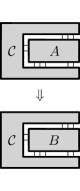
Figure 1: Replacing $A$ with $B$.

reflected in the analysis methodologies we use to tame their complexity. Indeed, in many cases the only way to go is to make use of compositional kinds of analysis, in which parts of a large system can be analysed in isolation, without having to care about the rest of the system, the environment. As an example, one could consider a component $A$ and replace it with another, e.g. more efficient component $B$ without looking at the context $\mathcal{C}$ in which $A$ and $B$ are supposed to operate, see Figure 1. Of course, for this program transformation to be safe, $A$ should be equivalent to $B$ or, at least, $B$ should be a refinement of $A$.

Program equivalences and refinements, indeed, are the cruxes of program semantics, and have been investigated in many different programming paradigms. When programs have an interactive behaviour, like in concurrent or higher-order languages, even defining a notion of program equivalence is not trivial, while coming out with handy methodologies for proving concrete programs to be equivalent can be quite challenging, and has been one of the major research topics in programming language theory, stimulating the development of techniques like logical relations [21, 18], applicative bisimilarity [1], and to some extent denotational semantics [24, 25] itself.

Coming back to our example, may we say anything about the case in which $A$ and $B$ are not equivalent, although behaving very similarly? Is there anything classic program semantics can say about this situation? Actually, the answer is negative: the program transformation turning such an $A$ into $B$ cannot be justified, simply because there is no guarantee about what the possible negative effects that turning $A$ into $B$ could have on the overall system formed by $\mathcal{C}$ and $A$. There are, however, many cases in which program transformations like the one we just described are indeed of interest, and thus desirable. Many examples can be, for instance, drawn from the field of approximate computing [19], in which equivalence-breaking program transformations are considered as beneficial provided the overall behaviour of the program is not affected too much by the transformation, while its intensional behaviour, e.g. its performance, is significantly improved.

One partial solution to the problem above consists in considering program metrics rather than program equivalences. This way, any pair of programs are dubbed being at a certain numerical distance rather than being merely equivalent (or not). This, for example, can be useful in the context of differential privacy [22, 5, 30] and has also been studied in the realms of domain theory [11, 4, 12, 14, 3] (see also [26] for an introduction to the subject) and coinduction [28, 27, 13, 7]. The common denominator among all these approaches is that on one hand, the notion of a congruence, crucial for compositional reasoning, is replaced by the one of a Lipschitz-continuous map: any context should not amplify (too much) the distance between any pair of terms, when it is fed with either the former or the latter:

$$\delta(C[M],C[N])\leq c\cdot\delta(M,N).$$

This enforces compositionality, and naturally leads us to consider metric spaces and Lipschitz functions as the underlying category. As is well known, this is not a cartesian closed category, and thus does not form a model of typed $\lambda$-calculi, unless one adopts linear type systems, or type systems in which the number of uses of each variable is kept track of, like $\mathsf{FUZZ}$ [22]. This somehow limits the compositionality of the metric approach [11, 15].

There are however program transformations which are intrinsically unjustifiable in the metric approach. Consider the following two programs of type $\mathit{REAL}\rightarrow\mathit{REAL}$

$$M_{\mathit{SIN}}:=\lambda x.\mathtt{sin}(x)\qquad\qquad M_{\mathit{ID}}:=\lambda x.x.$$

The two terms compute two very different functions on the real numbers, namely the sine trigonometric function and the identity on $\mathbb{R}$, respectively. The distance $\mid\sin x-x\mid$ is unbounded when $x$ ranges over $\mathbb{R}$. As a consequence, the numerical distance between $M_{\mathit{SIN}}$ and $M_{\mathit{ID}}$, however defined, is infinite, and the program transformation turning $M_{\mathit{SIN}}$ into $M_{\mathit{ID}}$ cannot be justified this way, for very good reasons. As highlighted by Westbrook and Chaudhuri [29], this is not the end of the story, at least if the environment in which $M_{\mathit{SIN}}$ and $M_{\mathit{ID}}$ operate feed either of them only with real numbers close to $0$, then $M_{\mathit{SIN}}$ can be substituted with $M_{\mathit{ID}}$ without affecting too much the overall behaviour of the system.

The key insight by Westbrook and Chaudhuri is that justifying program transformations like the one above requires taking the difference $\delta(M_{\mathit{SIN}},M_{\mathit{ID}})$ between $M_{\mathit{SIN}}$ and $M_{\mathit{ID}}$ not merely as a number, but as a more structured object. What they suggest is to take $\delta(M_{\mathit{SIN}},M_{\mathit{ID}})$ as yet another program, which however describes the difference between $M_{\mathit{SIN}}$ and $M_{\mathit{ID}}$:

$$\delta(M_{\mathit{SIN}},M_{\mathit{ID}}):=\lambda x.\lambda\varepsilon.|\sin x-x|+\varepsilon.$$

This reflects the fact that the distance between $M_{\mathit{SIN}}$ and $M_{\mathit{ID}}$, namely the discrepancy between their output, depends not only on the discrepancy on the input, namely on $\varepsilon$, but also on the input itself, namely on $x$. It both $x$ and $\varepsilon$ are close to $0$, $\delta(M_{\mathit{SIN}},M_{\mathit{ID}})$ is itself close to $0$.

In this paper, we develop Westbrook and Chaudhuri’s ideas, and turn them into a framework of differential logical relations. We will do all this in a simply-typed $\lambda$-calculus with real numbers as the only base type. Starting from such a minimal calculus has at least two advantages: on the one hand one can talk about meaningful examples like the one above, and on the other hand the induced metatheory is simple enough to highlight the key concepts.

The contributions of this paper can be summarised as follows:

• After introducing our calculus $\mathit{ST}^{\lambda}_{\mathbb{R}}$, we define differential logical relations inductively on types, as ternary relations between pairs of programs and differences. The latter are mere set theoretic entities here, and the nature of differences between terms depends on terms’ types.

• We prove a soundness theorem for differential logical relations, which allows us to justify compositional reasoning about terms’ differences. We also prove a finite difference theorem, which stipulates that the distance between two simply-typed $\lambda$-terms is finite if mild conditions hold on the underlying set of function symbols.

• We give embeddings of logical and metric relations into differential logical relations. This witnesses that the latter are a generalisation of the former two.

• Finally, we show that generalised metric domains, the mathematical structure underlying differential logical relations, form a cartesian closed category, contrarily to the category of metric spaces, which is well known not to have the same property.

Due to space constraints, many details have to be omitted, but can be found in an Extended Version of this work [10].

2 A Simply-Typed $\lambda$-Calculus with Real Numbers

In this section, we introduce a simply-typed $\lambda$-calculus in which the only base type is the one of real numbers, and constructs for iteration and conditional are natively available. The choice of this language as the reference calculus in this paper has been made for the sake of simplicity, allowing us to concentrate on the most crucial aspects, at the same time guaranteeing a minimal expressive power.

Terms and Types

$\mathit{ST}^{\lambda}_{\mathbb{R}}$ is a typed $\lambda$-calculus, so its definition starts by giving the language of types, which is defined as follows:

$$\tau,\rho::=\mathit{REAL}\mathbin{\bigl{|}}\tau\rightarrow\rho\mathbin{\bigl{|}}\tau\times\rho.$$

The expression $\tau^{n}$ stands for $\underbrace{\tau\times\cdots\times\tau}_{\mbox{$n$ times}}$. The set of terms is defined as follows:

$$M,N ::=x\mathbin{\bigl{|}}r\mathbin{\bigl{|}}f_{n}\mathbin{\bigl{|}}\lambda x.M\mathbin{\bigl{|}}MN\mathbin{\bigl{|}}\langle M,N\rangle\mathbin{\bigl{|}}\pi_{1}\;\;\mbox{\Large{$\mid$}}\;\;\pi_{2}\mathbin{\bigl{|}}\texttt{iflz}\;M\;\texttt{else}\;N\mathbin{\bigl{|}}\texttt{iter}\;M\;\texttt{base}\;N$$

where $x$ ranges over a set $\mathbb{V}$ of variables, $r$ ranges over the set $\mathbb{R}$ of real numbers, $n$ is a natural number and $f_{n}$ ranges over a set $\mathcal{F}_{n}$ of total real functions of arity $n$. We do not make any assumption on $\{\mathcal{F}_{n}\}_{n\in\mathbb{N}}$, apart from the predecessor $\mathit{pred}_{1}$ being part of $\mathcal{F}_{1}$. The family, in particular, could in principle contain non-continuous functions. The expression $\langle M_{1},\ldots,M_{n}\rangle$ is simply a shortcut for $\langle\ldots\langle\langle M_{1},M_{2}\rangle,M_{3}\rangle\ldots,M_{n}\rangle$. All constructs are self-explanatory, except for the $\mathtt{ifz}$ and $\mathtt{iter}$ operators, which are conditional and iterator combinators, respectively. An environment $\Gamma$ is a set of assignments of types to variables in $\mathbb{V}$ where each variable occurs at most once. A type judgment has the form $\Gamma\vdash M:\tau$ where $\Gamma$ is an environment, $M$ is a term, and $\tau$ is a type. Rules for deriving correct typing judgments are in Figure 2, and are standard.

$$\Gamma\vdash x:\tau x:\tau\in\Gamma\qquad\quad\Gamma\vdash r:\mathit{REAL}\qquad\quad\Gamma\vdash f_{n}:\mathit{REAL}^{n}\rightarrow\mathit{REAL}f_{n}\in\mathcal{F}_{n}\qquad\quad\Gamma\vdash\lambda x.M:\tau\rightarrow\rho\Gamma,x:\tau\vdash M:\rho$$ $$\Gamma\vdash MN:\rho\lx@proof@logical@and\Gamma\vdash M:\tau\rightarrow\rho\Gamma\vdash N:\tau\qquad\Gamma\vdash\langle M,N\rangle:\tau\times\rho\lx@proof@logical@and\Gamma\vdash M:\tau\Gamma\vdash N:\rho\qquad\Gamma\vdash\pi_{1}:\tau\times\rho\rightarrow\tau\qquad\Gamma\vdash\pi_{2}:\tau\times\rho\rightarrow\rho$$ $$\Gamma\vdash\texttt{iflz}\;M\;\texttt{else}\;N:\mathit{REAL}\rightarrow\tau\lx@proof@logical@and\Gamma\vdash M:\tau\Gamma\vdash N:\tau\qquad\qquad\qquad\Gamma\vdash\texttt{iter}\;M\;\texttt{base}\;N:\mathit{REAL}\rightarrow\tau\lx@proof@logical@and\Gamma\vdash M:\tau\rightarrow\tau\Gamma\vdash N:\tau$$

Figure 2: Typing rules for $\mathit{ST}^{\lambda}_{\mathbb{R}}$.

The set of terms $M$ for which $\cdot\vdash M:\tau$ is derivable is indicated as $\mathit{CT}({\tau})$.

Call-by-Value Operational Semantics

A static semantics is of course not enough to give meaning to a paradigmatic programming language, the dynamic aspects being captured only once an operational semantics is defined. The latter turns out to be very natural. Values are defined as follows:

$$V,W::=r\mathbin{\bigl{|}}f_{n}\mathbin{\bigl{|}}\lambda x.M\mathbin{\bigl{|}}\langle M,N\rangle\mathbin{\bigl{|}}\pi_{1}\mathbin{\bigl{|}}\pi_{2}\mathbin{\bigl{|}}\texttt{iflz}\;M\;\texttt{else}\;N\mathbin{\bigl{|}}\texttt{iter}\;M\;\texttt{base}\;N$$

The set of closed values of type $\tau$ is $\mathit{CV}({\tau})\subseteq\mathit{CT}({\tau})$, and the evaluation of $M\in\mathit{CT}({\tau})$ produces a value $V\in\mathit{CV}({\tau})$, as formalised by the rules in Figure 3, through the judgment $M\Downarrow V$.

$$V\Downarrow V\qquad MN\Downarrow f(r_{1},\ldots,r_{n})\lx@proof@logical@and M\Downarrow f_{n}N\Downarrow\langle L_{1},\ldots,L_{n}\rangle L_{i}\Downarrow r_{i}\qquad MN\Downarrow W\lx@proof@logical@and M\Downarrow\lambda x.LN\Downarrow VL\{V/x\}\Downarrow W$$ $$MN\Downarrow V\lx@proof@logical@and M\Downarrow\pi_{1}N\Downarrow\langle L,P\rangle L\Downarrow V\qquad MN\Downarrow V\lx@proof@logical@and M\Downarrow\pi_{2}N\Downarrow\langle L,P\rangle P\Downarrow V$$ $$MN\Downarrow V\lx@proof@logical@and M\Downarrow\texttt{iflz}\;L\;\texttt{else}\;PN\Downarrow rr<0L\Downarrow V\qquad MN\Downarrow V\lx@proof@logical@and M\Downarrow\texttt{iflz}\;L\;\texttt{else}\;PN\Downarrow rr\geq 0P\Downarrow V$$ $$MN\Downarrow V\lx@proof@logical@and M\Downarrow\texttt{iter}\;L\;\texttt{base}\;PN\Downarrow rr<0P\Downarrow V$$ $$MN\Downarrow V\lx@proof@logical@and M\Downarrow\texttt{iter}\;L\;\texttt{base}\;PN\Downarrow rr\geq 0L((\texttt{iter}\;L\;\texttt{base}\;P)(\mathit{pred}_{1}(r))\Downarrow V$$

Figure 3: Operational semantics for $\mathit{ST}^{\lambda}_{\mathbb{R}}$.

We write $M\Downarrow$ if $M\Downarrow V$ is derivable for some $V$. The absence of full recursion has the nice consequence of guaranteeing a form of termination:

Thoerem 1.

The calculus $\mathit{ST}^{\lambda}_{\mathbb{R}}$ is terminating: if ${\cdot\vdash M:\tau}$ then $M\Downarrow$.

We show the normalisation theorem using the standard reducibility candidate argument.

Definition 2.

We define $\mathit{RED}_{\tau}$ as follows.

$$\mathit{RED}_{\tau} =\{M\;\mid\;M\Downarrow V\land V\in\mathit{VRED}_{\tau}\}$$

$$\mathit{VRED}_{\mathit{REAL}} =\mathbb{R}$$

$$\mathit{VRED}_{\tau\rightarrow\rho} =\{V\;\mid\;\forall W\in\mathit{VRED}_{\tau}.VW\in\mathit{RED}_{\rho}\}$$

$$\mathit{VRED}_{\tau\times\rho} =\{\langle M,N\rangle\;\mid\;M\in\mathit{RED}_{\tau}\land N\in\mathit{RED}_{\rho}\}$$

Then we show the two lemmas that prove Theorem 1 together:

Lemma 3.

If ${\cdot\vdash M:\tau}$, then $M\in\mathit{RED}_{\tau}$.

Proof.

The following strengthening of the statement can be proved by incuction on the structure of $M$: whenever ${x_{1}:\rho_{1},\ldots,x_{n}:\rho_{n}\vdash M:\tau}$ and whenever $V_{i}\in\mathit{VRED}_{\rho_{i}}$ it holds that

$$M\{V_{1}/x_{1},\ldots,V_{n}/x_{n}\}\in\mathit{RED}_{\tau}.$$

All inductive cases are standard. One that deserves a little bit of attentionis the case of abstractions, in which one needs to deduce that $(\lambda x.M)V\in\mathit{RED}_{\tau}$ iff $M\{x/V\}\in\mathit{RED}_{\tau}$. But this is of course easy to prove, because the former evaluated to any value $W$ iff the latter evaluates to $W$. Another delicate case is the one of $\texttt{iter}\;M\;\texttt{base}\;N$, which requires an induction. ∎

Please observe that, by definition, if $M\in\mathit{RED}_{\tau}$, then $M\Downarrow$. As a consequence, one easily gets termination from Lemma 3.

Corollary 4.

If ${\cdot\vdash M:\mathit{REAL}}$ then there exists a unique $r\in\mathbb{R}$ satisfying $M\Downarrow r$, which we indicate as $\mathit{NF}({M})$.

Proof.

By Theorem 1 there exists a value $V$ satisfying $M\Downarrow V$. The only form of value of type $\mathit{REAL}$ is $r\in\mathbb{R}$. Moreover, the fact that such a $r$ is unique is a consequence of the following, slightly more general result: if $M\Downarrow V$ and $M\Downarrow W$, then $V$ is syntactically equal to $W$. This can be proved by a straightforward induction on the structure of the proof that, e.g., $M\Downarrow V$. ∎

Context Equivalence

A context $C$ is nothing more than a term containing a single occurrence of a placeholder $[\cdot]$. Given a context $C$, $C[M]$ indicates the term one obtains by substituting $M$ for the occurrence of $[\cdot]$ in $C$. Typing rules in Figure 2 can be lifted to contexts by a generalising judgments to the form $\Gamma\vdash C[\Delta\vdash\cdot:\tau]:\rho$, by which one captures that whenever $\Delta\vdash M:\tau$ it holds that $\Gamma\vdash C[M]:\rho$. Two terms $M$ and $N$ such that $\Gamma\vdash M,N:\tau$ are said to be context equivalent [20] when for every $C$ such that $\emptyset\vdash C[\Gamma\vdash\cdot:\tau]:\mathit{REAL}$ it holds that $\mathit{NF}({C[M]})=\mathit{NF}({C[N]})$. Context equivalence is the largest adequate congruence, and is thus considered as the coarsest “reasonable” equivalence between terms. It can also be turned into a pseudometric [9, 8] — called context distance — by stipulating that

$$\delta(M,N)=\sup_{\emptyset\vdash C[\Gamma\vdash\cdot:\tau]:\mathit{REAL}}|\mathit{NF}({C[M]})-\mathit{NF}({C[M]})|.$$

The obtained notion of distance, however, is bound to trivialise [9], given that $\mathit{ST}^{\lambda}_{\mathbb{R}}$ is not affine. Trivialisation of context distance highlights an important limit of the metric approach to program difference which, ultimately, can be identified with the fact that program distances are sensitive to interactions with the environment. Our notion of a differential logical relation tackles such a problem from a different perspective, namely refining the concept of a program difference which is not just a number, but is now able to take into account interactions with the environment.

Set-Theoretic Semantics

Before introducing differential logical relations, it is useful to remark that we can give $\mathit{ST}^{\lambda}_{\mathbb{R}}$ a standard set-theoretic semantics. To any type $\tau$ we associate the set $\llbracket\tau\rrbracket$, the latter being defined by induction on the structure of $\tau$ as follows:

$$\llbracket\mathit{REAL}\rrbracket=\mathbb{R};\qquad\qquad\llbracket\tau\rightarrow\rho\rrbracket=\llbracket\tau\rrbracket\rightarrow\llbracket\rho\rrbracket;\qquad\qquad\llbracket\tau\times\rho\rrbracket=\llbracket\tau\rrbracket\times\llbracket\rho\rrbracket.$$

This way, any closed term $M\in\mathit{CT}({\tau})$ is interpreted as an element $\llbracket M\rrbracket$ of $\llbracket\tau\rrbracket$ in a natural way (see, e.g. [18]). Up to now, everything we have said about $\mathit{ST}^{\lambda}_{\mathbb{R}}$ is absolutely standard, and only serves to set the stage for the next sections.

3 Making Logical Relations Differential

Logical relations can be seen as one of the many ways of defining when two programs are to be considered equivalent. Their definition is type driven, i.e., they can be seen as a family $\{\delta_{\tau}\}_{\tau}$ of binary relations indexed by types such that $\delta_{\tau}\subseteq\mathit{CT}({\tau})\times\mathit{CT}({\tau})$. This section is devoted to showing how all this can be made into differential logical relations.

The first thing that needs to be discussed is how to define the space of differences between programs. These are just boolean values in logical relations, become real numbers in ordinary metrics, and is type-dependent itself here. A function $\llparenthesis{\cdot}\rrparenthesis$ that assigns a set to each type is defined as follows:

$$\llparenthesis{\mathit{REAL}}\rrparenthesis=\mathbb{R}_{\geq 0}^{\infty};\qquad\qquad\llparenthesis{\tau\rightarrow\rho}\rrparenthesis=\llbracket\tau\rrbracket\times\llparenthesis{\tau}\rrparenthesis\rightarrow\llparenthesis{\rho}\rrparenthesis;\qquad\qquad\llparenthesis{\tau\times\rho}\rrparenthesis=\llparenthesis{\tau}\rrparenthesis\times\llparenthesis{\rho}\rrparenthesis;$$

where $\mathbb{R}_{\geq 0}^{\infty}=\mathbb{R}_{\geq 0}\cup\{\infty\}$. The set $\llparenthesis{\tau}\rrparenthesis$ is said to be the difference space for the type $\tau$ and is meant to model the outcome of comparisons between closed programs of type $\tau$. As an example, when $\tau$ is $\mathit{REAL}\rightarrow\mathit{REAL}$, we have that $\llparenthesis{\tau}\rrparenthesis=\mathbb{R}\times\mathbb{R}_{\geq 0}^{\infty}\rightarrow\mathbb{R}_{\geq 0}^{\infty}$. This is the type of the function $\delta(M,N)$ we used to compare the two programs described in the Introduction.

Now, which structure could we endow $\llparenthesis{\tau}\rrparenthesis$ with? First of all, we can define a partial order ${\leq_{\tau}}$ over $\llparenthesis{\tau}\rrparenthesis$ for each type $\tau$ as follows:

$$r \leq_{\mathit{REAL}}s \text{ if }r\leq s\text{ as the usual order over $\mathbb{R}_{\geq 0}^{\infty}$};$$

$$f \leq_{\tau\rightarrow\rho}g \text{ if }\forall x\in\llbracket\tau\rrbracket.\forall t\in\llparenthesis{\tau}\rrparenthesis.f(x,t)\leq_{\rho}g(x,t);$$

$$(t,u) \leq_{\tau\times\rho}(s,r) \text{ if }t\leq_{\tau}s\text{ and }u\leq_{\rho}r.$$

This order has least upper bounds and greater lower bounds, thanks to the nice structure of $\mathbb{R}_{\geq 0}^{\infty}$:

Proposition 5.

For each type $\tau$, $(\llparenthesis{\tau}\rrparenthesis,\leq_{\tau})$ forms a complete lattice.

Proof.

We show that each $\llparenthesis{\tau}\rrparenthesis$ has suprema by induction on types.

• Case $\mathit{REAL}$. Then $(\llparenthesis{\tau}\rrparenthesis,\leq_{\tau})=(\mathbb{R}_{\geq 0}^{\infty},\leq)$ is clearly complete.

• Case $\tau\rightarrow\rho$. Given a subset $A\subseteq\llparenthesis{\tau\rightarrow\rho}\rrparenthesis$, we define $s_{A}\in\llparenthesis{\tau\rightarrow\rho}\rrparenthesis$ as:

  $$s_{A}(V,t)=\sup_{f\in A}f(V,t),$$

  where the supremum on the right-hand side exists by induction hypothesis (on the type $\rho$). This $s_{A}$ serves as the supremum of $A$ because:

  • (Upperbound.) For any $g\in A$, by definition of supremum it holds that:

    $\forall V\in\mathit{CV}({\tau}).\forall t\in\llparenthesis{\tau}\rrparenthesis.g(V,t)\leq_{\tau}\sup_{f\in A}f(V,t)=s_{A}(V,t)$. Hence $g\leq_{\tau\rightarrow\rho}s_{A}$.

  • (Leastness.) Suppose that $s^{\prime}$ is an upperbound of $A$, i.e. $\forall f\in A.f\leq_{\tau\rightarrow\rho}s^{\prime}$. Then, it by definition means that: $\forall f\in A.\forall V\in\mathit{CV}({\tau}).\forall t\in\llparenthesis{\tau}\rrparenthesis.f(V,t)\leq_{\rho}s^{\prime}(V,t).$ Therefore $s^{\prime}(V,t)$ is an upperbound of the set $\{f(V,t)\}_{f\in A}$ for each $V,t$. Thus by definition of supremum, $s_{A}(V,t)=\sup_{f\in A}f(V,t)\leq_{\rho}s^{\prime}(V,t)$ for each $V,t$. Hence $s_{A}\leq_{\tau\rightarrow\rho}s^{\prime}$ holds by definition of $\leq_{\tau\rightarrow\rho}$.

• Case $\tau\times\rho$. Given a subset $A\subseteq\llparenthesis{\tau\times\rho}\rrparenthesis$, we define $s_{A}=(\sup\boldsymbol{\pi_{1}}A,\sup\boldsymbol{\pi_{2}}A)\in\llparenthesis{\tau\times\rho}\rrparenthesis$, where $\boldsymbol{\pi_{1}}$ and $\boldsymbol{\pi_{2}}$ are meta-level projections and the suprema on the right-hand side exist by induction hypothesis (on the types $\tau$ and $\rho$). One can verify that $s_{A}$ is the supremum of $A$ in a straightforward way:

  • (Upperbound.) For any $(t,u)\in A$, by definition of supremum $t\leq_{\tau}\sup\boldsymbol{\pi_{1}}A$ and $u\leq_{\rho}\sup\boldsymbol{\pi_{2}}A$ hold. Hence $(t,u)\leq_{\tau\times\rho}(\sup\boldsymbol{\pi_{1}}A,\sup\boldsymbol{\pi_{2}}A)=s_{A}$ by definition of $\leq_{\tau\times\rho}$.

  • (Leastness.) Suppose that $(s^{\prime}_{1},s^{\prime}_{2})$ is an upperbound of $A$, i.e.

    $\forall(t_{1},t_{2})\in A.(t_{1},t_{2})\leq_{\tau\times\rho}(s^{\prime}_{1},s^{\prime}_{2})$. It by definition means that $\forall t_{1}\in\boldsymbol{\pi_{1}}A.t_{1}\leq_{\tau}s^{\prime}_{1}$ and $\forall t_{2}\in\boldsymbol{\pi_{2}}A.t_{2}\leq_{\rho}s^{\prime}_{2}$. Therefore $s^{\prime}_{1}$ (resp. $s^{\prime}_{2}$) is an upperbound of the set $\boldsymbol{\pi_{1}}A$ (resp. $\boldsymbol{\pi_{2}}A$). Thus by definition of supremum, $\sup\boldsymbol{\pi_{1}}A\leq_{\tau}s^{\prime}_{1}$ (resp. $\sup\boldsymbol{\pi_{2}}A\leq_{\rho}s^{\prime}_{2}$). Hence $(\sup\boldsymbol{\pi_{1}}A,\sup\boldsymbol{\pi_{2}}A)\leq_{\tau\times\rho}(s^{\prime}_{1},s^{\prime}_{2})$ holds by definition of $\leq_{\tau\times\rho}$.

∎

The fact that $\llparenthesis{\tau}\rrparenthesis$ has a nice order-theoretic structure is not the end of the story. For every type $\tau$, we define a binary operation $*_{\tau}$ as follows:

$$r*_{\mathit{REAL}}s \stackrel{{\scriptstyle\text{def.}}}{{=}}r+s\mbox{ if }r,s\in\mathbb{R}_{\geq 0}; (f*_{\tau\rightarrow\rho}g)(V,t) \stackrel{{\scriptstyle\text{def.}}}{{=}}f(V,t)*_{\rho}g(V,t);$$

$$r*_{\mathit{REAL}}s \stackrel{{\scriptstyle\text{def.}}}{{=}}\infty\mbox{ if }r=\infty\vee s=\infty; (t,s)*_{\tau\times\rho}(u,r) \stackrel{{\scriptstyle\text{def.}}}{{=}}(t*_{\tau}u,s*_{\rho}r).$$

This is precisely what it is needed to turn $\llparenthesis{\tau}\rrparenthesis$ into a quantale [23].

Proposition 6.

For each type $\tau$, $\llparenthesis{\tau}\rrparenthesis$ forms a commutative unital non-idempotent quantale. That is, the following holds for any $\tau$:

• $t*_{\tau}u=u*_{\tau}t$ for all $t,u\in\llparenthesis{\tau}\rrparenthesis$,

• $t*_{\tau}(\sup_{i\in I}u_{i})=\sup_{i\in I}(t*_{\tau}u_{i})$ for all $t,u_{i}\in\llparenthesis{\tau}\rrparenthesis$ where $I$ is an arbitrary index set,

• there exists an element $e_{\tau}\in\llparenthesis{\tau}\rrparenthesis$ satisfying $e_{\tau}*_{\tau}t=t$ for all $t\in\llparenthesis{\tau}\rrparenthesis$,

• $*_{\tau}$ does not necessarily satisfy $t*_{\tau}t=t$.

Proof.

By induction on $\tau$.

• Case $\mathit{REAL}$. The multiplication $*_{\mathit{REAL}}$ is clearly commutative and satisfies $r*_{\tau}(\sup_{i\in I}s_{i})=\sup_{i\in I}(r*_{\tau}s_{i})$ for all $r,s_{i}\in\llparenthesis{\mathit{REAL}}\rrparenthesis=\mathbb{R}_{\geq 0}^{\infty}$. The unit $e_{\mathit{REAL}}$ is $0$; the multiplication is obviously non-idempotent.

• Case $\tau\rightarrow\rho$. It holds that $(f*_{\tau\rightarrow\rho}g)=(g*_{\tau\rightarrow\rho}f)$ because

  $$\begin{array}[]{ll}(f*_{\tau\rightarrow\rho}g)(V,t)&=f(V,t)*_{\rho}g(V,t)\\ &\stackrel{{\scriptstyle\text{I.H.}}}{{=}}g(V,t)*_{\rho}f(V,t)\\ &=(g*_{\tau\rightarrow\rho}f)(V,t)\end{array}$$

  and $f*_{\tau\rightarrow\rho}(\sup_{i\in I}(g_{i}))=\sup_{i\in I}(f*_{\tau\rightarrow\rho}g_{i})$ because

  $$\begin{array}[]{ll}(f*_{\tau\rightarrow\rho}(\sup_{i\in I}(g_{i})))(V,t)&=f(V,t)*_{\rho}(\sup_{i\in I}g_{i})(V,t)\\ &=f(V,t)*_{\rho}(\sup_{i\in I}(g_{i}(V,t)))\\ &\stackrel{{\scriptstyle\text{I.H.}}}{{=}}\sup_{i\in I}(f(V,t)*_{\rho}g_{i}(V,t))\\ &=\sup_{i\in I}((f*_{\tau\rightarrow\rho}g_{i})(V,t))\\ &=(\sup_{i\in I}(f*_{\tau\rightarrow\rho}g_{i}))(V,t).\end{array}$$

  The unit $e_{\tau\rightarrow\rho}$ is the constant $e_{\rho}$ function: $e_{\tau\rightarrow\rho}(V,t)=e_{\rho}$ for all $V,t$.

• Case $\tau\times\rho$. Then

  $$\begin{array}[]{ll}(t,t^{\prime})*_{\tau\times\rho}(u,u^{\prime})&=(t*_{\tau}u,t^{\prime}*_{\rho}u^{\prime})\\ &\stackrel{{\scriptstyle\text{I.H.}}}{{=}}(u*_{\tau}t,u^{\prime}*_{\rho}t^{\prime})\\ &=(u,u^{\prime})*_{\tau\times\rho}(t,t^{\prime})\end{array}$$

  and

  $$\begin{array}[]{ll}(t,t^{\prime})*_{\tau\times\rho}(\sup_{i\in I}(u_{i},u^{\prime}_{i}))&=(t,t^{\prime})*_{\tau\times\rho}(\sup_{i\in I}u_{i},\sup_{i\in I}u^{\prime}_{i})\\ &=(t*_{\tau}(\sup_{i\in I}u_{i}),t^{\prime}*_{\tau}(\sup_{i\in I}u^{\prime}_{i}))\\ &\stackrel{{\scriptstyle\text{I.H.}}}{{=}}(\sup_{i\in I}(t*_{\tau}u_{i}),\sup_{i\in I}(t^{\prime}*_{\tau}u^{\prime}_{i}))\\ &=\sup_{i\in I}(t*_{\tau}u_{i},t^{\prime}*_{\tau}u^{\prime}_{i})\\ &=\sup_{i\in I}\left((t,t^{\prime})*_{\tau\times\rho}(u_{i},u^{\prime}_{i})\right).\end{array}$$

  The unit $e_{\tau\times\rho}$ is $(e_{\tau},e_{\rho})$.

∎

The fact that $\llparenthesis{\tau}\rrparenthesis$ is a quantale means that it has, e.g., the right structure to be the codomain of generalised metrics [17, 16]. Actually, a more general structure is needed for our purposes, namely the one of a generalised metric domain, which will be thoroughly discussed in Section 6 below. For the moment, let us concentrate our attention to programs:

Definition 7 (Differential Logical Relations).

We define a differential logical relation $\{\delta_{\tau}\subseteq\Lambda_{\tau}\times\llparenthesis{\tau}\rrparenthesis\times\Lambda_{\tau}\}_{\tau}$ as a set of ternary relations indexed by types satisfying

$$\delta_{\mathit{REAL}}({M},{r},{N})\Leftrightarrow \;|\mathit{NF}({M})-\mathit{NF}({N})|\leq r;$$

$$\delta_{\tau\times\rho}({M},{(d_{1},d_{2})},{N})\Leftrightarrow \;\delta_{\tau}({\pi_{1}M},{d_{1}},{\pi_{1}N})\land\delta_{\rho}({\pi_{2}M},{d_{2}},{\pi_{2}N})$$

$$\delta_{\tau\rightarrow\rho}({M},{d},{N})\Leftrightarrow \;(\forall V\in\mathit{CV}({\tau}).\ \forall x\in\llparenthesis{\tau}\rrparenthesis.\ \forall W\in\mathit{CV}({\tau}).\$$

$$\,\,\delta_{\tau}({V},{x},{W})\Rightarrow\delta_{\rho}({MV},{d(\llbracket V\rrbracket,x)},{NW})\land\delta_{\rho}({MW},{d(\llbracket V\rrbracket,x)},{NV})).$$

An intuition behind the condition required for $\delta_{\tau\rightarrow\rho}({M},{d},{N})$ is that $d(\llbracket V\rrbracket,y)$ overapproximates both the “distance” between $MV$ and $NW$ and the one between $MW$ and $NV$, this whenever $W$ is within the error $x$ from $V$.

Some basic facts about differential logical relations, which will be useful in the following are now in order.

Lemma 8.

For every $\tau,M,N$, it holds that $\delta_{\tau}({M},{d},{N})$ if and only if $\delta_{\tau}({N},{d},{M})$.

Proof.

By induction on types. ∎

Lemma 9.

Let $\cdot\vdash M,N:\tau$ and $d\in\llparenthesis{\tau}\rrparenthesis$. Assume that $\delta_{\mathit{REAL}}({M},{d},{N})$ and $\delta_{\mathit{REAL}}({N},{e},{L})$ implies $\delta_{\mathit{REAL}}({M},{d+e},{L})$. Then $\delta_{\tau}({M},{d},{N})$ and $\delta_{\tau}({N},{e},{L})$ implies $\delta_{\tau}({M},{d+e},{L})$.

Proof.

By induction on types. ∎

Lemma 10.

Let $\cdot\vdash M,N:\tau$ and $d\in\llparenthesis{\tau}\rrparenthesis$. Assume that $\delta_{\mathit{REAL}}({M},{d},{N})$ and $d\leq e$ implies $\delta_{\mathit{REAL}}({M},{e},{N})$. Then $\delta_{\tau}({M},{d},{N})$ and $d\leq e$ implies $\delta_{\tau}({M},{e},{N})$.

Proof.

By induction on types. ∎

3.1 A Fundamental Lemma

Usually, the main result about any system of logical relations is the so-called Fundamental Lemma, which states that any typable term is in relation with itself. But how would the Fundamental Lemma look like here? Should any term be at somehow minimal distance to itself, in the spirit of what happens, e.g. with metrics [22, 11]? Actually, there is no hope to prove anything like that for differential logical relations, as the following example shows.

Example 11.

Consider again the term $M_{\mathit{ID}}=\lambda x.x$, which can be given type $\tau=\mathit{REAL}\rightarrow\mathit{REAL}$ in the empty context. Please recall that $\llparenthesis{\tau}\rrparenthesis=\mathbb{R}\times\mathbb{R}_{\geq 0}^{\infty}\rightarrow\mathbb{R}_{\geq 0}^{\infty}$. Could we prove that $\delta_{\tau}(M_{\mathit{ID}},0_{\tau},M_{\mathit{ID}})$, where $0_{\tau}$ is the constant-$0$ function? The answer is negative: given two real numbers $r$ and $s$ at distance $\varepsilon$, the terms $M_{\mathit{ID}}r$ and $M_{\mathit{ID}}s$ are themselves $\varepsilon$ apart, thus at nonnull distance. The best one can say, then, is that $\delta_{\tau}(M_{\mathit{ID}},f,M_{\mathit{ID}})$, where $f(x,\varepsilon)=\varepsilon$.

As the previous example suggests, a term $M$ being at self-distance $d$ is a witness of $M$ being sensitive to changes to the environment according to $d$. Indeed, the only terms which are at self-distance $0$ are the constant functions. This makes the underlying theory more general than the one of logical or metric relations, although the latter can be proved to be captured by differential logical relations, as we will see in the next section.

Coming back to the question with which we opened the section, we can formulate a suitable fundamental lemma for differential logical relations by stating that for any closed term $M$ of type $\tau$ there exists $d\in\llparenthesis{\tau}\rrparenthesis$ such that $(M,d,M)\in\delta_{\tau}$. In order to prove such result, however, we need to prove something stronger, namely the extension of the above statement to arbitrary (and thus possibly open) terms. Doing so, requires to extend differential logical relations to arbitrary sequents $\Gamma\vdash\tau$.

Let us begin extending the maps $\llbracket\cdot\rrbracket$ and $\llparenthesis{\cdot}\rrparenthesis$ to environments.

Definition 12.

Given an environment $\Gamma$, define:

$$\llbracket\Gamma\rrbracket=\prod_{(x:\tau)\in\Gamma}\llbracket\tau\rrbracket;\qquad\llparenthesis{\Gamma}\rrparenthesis=\prod_{(x:\tau)\in\Gamma}\llparenthesis{\tau}\rrparenthesis.$$

An element in e.g. $\llparenthesis{\Gamma}\rrparenthesis$ is thus a family $\alpha\in\prod_{(x:\tau)\in\Gamma}$, meaning that for any $(x:\tau)\in\Gamma$, $\alpha(x)\in\llparenthesis{\tau}\rrparenthesis$. The syntactic counterparts of such families is given by families $\mathbf{V}\in\prod_{(x:\tau)\in\Gamma}\mathit{CV}({\tau})$. We refer to $\mathbf{V}$ as a $\Gamma$-family of values. Indeed, such a $\Gamma$-family of values can naturally be seen as a substitution mapping each variable $(x:\tau)\in\Gamma$ to $\mathbf{V}(x)\in\mathit{CV}({\tau})$. As it is customary, for a term $\Gamma\vdash M:\tau$ we write $M\mathbf{V}$ for the closed term of type $\tau$ obtained applying the substitution $\mathbf{V}$ to $M$. We denote by $\mathit{CV}({\Gamma})$ the set of all $\Gamma$-family of values.

We can now extend a differential logical relation $\{\delta_{\tau}\}_{\tau}$ to environments stipulating that the family $\{\delta_{\Gamma}\subseteq\mathit{CV}({\Gamma})\times\llparenthesis{\Gamma}\rrparenthesis\times\mathit{CV}({\Gamma})\}_{\Gamma}$ is a differential logical relation if

$$\delta_{\Gamma}(\mathbf{V},\alpha,\mathbf{W})\iff\forall(x:\tau)\in\Gamma.\ \delta_{\tau}(\mathbf{V}(x),\alpha(x),\mathbf{W}(x)).$$

Next, we extend our framework to arbitrary sequents $\Gamma\vdash\tau$. First of all, we define:

$$\llbracket\Gamma\vdash\tau\rrbracket=\llbracket\tau\rrbracket^{\llbracket\Gamma\rrbracket}\qquad\llparenthesis{\Gamma\vdash\tau}\rrparenthesis=\llparenthesis{\tau}\rrparenthesis^{\llbracket\Gamma\rrbracket\times\llparenthesis{\Gamma}\rrparenthesis}.$$

It is then natural to extend $\{\delta_{\tau}\}_{\tau}$ to arbitrary sequents by stipulating that $\{\delta_{\Gamma\vdash\tau}\subseteq\Lambda_{\Gamma\vdash\tau}\times\llparenthesis{\Gamma\vdash\tau}\rrparenthesis\times\Lambda_{\Gamma\vdash\tau}\}_{\Gamma\vdash\tau}$, where $\Lambda_{\Gamma\vdash\tau}$ denotes the set of sequents typable within the sequent $\Gamma\vdash\tau$, is a differential logical relation if $\delta_{\Gamma\vdash\tau}(M,d,N)$ holds if and only if

$$\delta_{\Gamma}({\mathbf{V}},{\alpha},{\mathbf{W}})\implies\delta_{\tau}({M\mathbf{V}},{d(\llbracket\mathbf{V}\rrbracket,\alpha)},{N\mathbf{W}}).$$

This definition as it is, however, does not work well, as it does not take into account possible alternations of the substitutions $\mathbf{V}$ and $\mathbf{W}$. To solve this issue we introduce the following notation. Given a boolean-valued map $B\in\{0,1\}^{\Gamma}$, and two substitutions $\mathbf{V},\mathbf{W}\in\mathit{CV}({\Gamma})$, define the substitution ${B}^{\mathbf{V}}_{\mathbf{W}}\in\mathit{CV}({\Gamma})$ as:

$${B}^{\mathbf{V}}_{\mathbf{W}}(x)=\left\{\begin{array}[]{ll}\mathbf{V}(x)&\mbox{if $b(x)=0$}\\ \mathbf{W}(x)&\mbox{if $b(x)=1$}.\\ \end{array}\right.$$

We can now extend differential logical relations to arbitrary terms.

Definition 13.

Given a differential logical relations $\{\delta_{\tau}\}_{\tau}$, define $\{\delta_{\Gamma\vdash\tau}\subseteq\Lambda_{\Gamma\vdash\tau}\times\llparenthesis{\Gamma\vdash\tau}\rrparenthesis\times\Lambda_{\Gamma\vdash\tau}\}_{\Gamma\vdash\tau}$ stipulating that $\delta_{\Gamma\vdash\tau}(M,d,N)$ holds if and only if

$$\delta_{\Gamma}({\mathbf{V}},{\alpha},{\mathbf{W}})\implies\forall B\in\{0,1\}^{\Gamma}\delta_{\tau}({M{B}^{\mathbf{V}}_{\mathbf{W}}},{d(\llbracket\mathbf{V}\rrbracket,\alpha)},{N{B}^{\mathbf{W}}_{\mathbf{V}}}).$$

Before proving the desired strengthening of the fundamental lemma, it is useful to observe the following useful result.

Lemma 14.

For all terms $\cdot\vdash M,N:\tau$, we have $\delta_{\tau}(M,d,N)\iff\delta_{\tau}(NF(M),d,NF(N))$.

Proof.

First observe that if $\delta_{\tau}(M^{\prime},d,N)$ and $M\to_{\beta}M^{\prime}$ (where $\to_{\beta}$ is the obvious small-step semantics relation associated to $\Downarrow$), then $\delta_{\tau}(M,d,N)$ holds (a similar statement holds for $N$). By Theorem  1 we thus infer the right-to-left implication. For the other implication, we proceed by induction on $\tau$ observing that $NF(NF(M)V)=NF(MV)$. ∎

Lemma 15.

For any $\Gamma\vdash M:\tau$, there exists $d\in\llparenthesis{\Gamma\vdash\tau}\rrparenthesis$ such that $\delta_{\Gamma\vdash\tau}(\tau,d,\tau)$ holds.

Proof.

The proof is by induction on $\Gamma\vdash M:\tau$.

• Suppose $\Gamma\vdash x:\tau$, meaning that $x\in\Gamma$. We simply define $d:\llbracket\Gamma\rrbracket\times\llparenthesis{\Gamma}\rrparenthesis\to\llparenthesis{\tau}\rrparenthesis$ as $d(g,\alpha)=\alpha(x)$.

• Suppose $\Gamma\vdash r:\mathit{REAL}$. Define $d:\llbracket\Gamma\rrbracket\times\llparenthesis{\Gamma}\rrparenthesis\to\mathbb{R}_{\geq 0}^{\infty}$ as $d(g,\alpha)=0$.

• Suppose $\Gamma\vdash f:\mathit{REAL}^{n}\to\mathit{REAL}$. For simplicity, we show the case for $n=1$ (the case for $n>1$ follows the same structure). We have to find $d\in\llparenthesis{\mathit{REAL}\to\mathit{REAL}}\rrparenthesis^{\llbracket\Gamma\rrbracket\times\llparenthesis{\Gamma}\rrparenthesis}$ such that $\delta_{\Gamma}(\mathbf{V},\alpha,\mathbf{W})$ implies $\delta_{\mathit{REAL}\to\mathit{REAL}}(f,d(\llbracket\mathbf{V}\rrbracket,\alpha),f)$. The latter means, that for all values $\cdot\vdash V,W\vdash\mathit{REAL}$ (for simplicity, we denote by $V$ both the numeral $V$ and the number $\llbracket V\rrbracket$) and $e\in\mathbb{R}_{\geq 0}^{\infty}$, $|V-W|\leq e$ implies $|NF(f(V))-NF(f(W))|\leq d(\llbracket\mathbf{V}\rrbracket,\alpha)(V,e)$. Define:

  $$A=\bigcup_{e^{\prime}\in\mathbb{R},e^{\prime}\leq e}[V-e^{\prime},V+e^{\prime}];\qquad d(\llbracket\mathbf{V}\rrbracket,\alpha)(\llbracket V\rrbracket,e)=diam(f(A)),$$

  where the diameter $diam(X)$ of a set $X\subseteq\mathbb{R}$ is defined as $\sup_{x,y\in X}|x-y|$. Notice that a set can have diameter $\infty$. We conclude the wished thesis observing that $|V-W|\leq e$ implies $V,W\in A$ (recall that $V,W$ being real numbers, so is $|V-W|$), and thus $f(V),f(W)\in f(A)$. As a consequence, $|f(V)-f(W)|\leq diam(f(A))$, and thus we are done.

• Suppose $\Gamma\vdash MN:\tau\lx@proof@logical@and\Gamma\vdash M:\rho\to\tau\Gamma\vdash N:\rho$ . By induction hypothesis we have:

  1. There exists $d_{1}\in\llparenthesis{\rho\to\tau}\rrparenthesis^{\llbracket\Gamma\rrbracket\times\llparenthesis{\Gamma}\rrparenthesis}$ such that $\delta_{\Gamma}(\mathbf{V},\alpha,W)$ implies for any $B\in\{0,1\}^{\Gamma}$, for all $V,W\in CV(\rho)$, and for any $x\in\llparenthesis{\rho}\rrparenthesis$:

     $$\delta_{\rho}(V,x,W)\implies\delta_{\tau}(M{B}^{\mathbf{V}}_{\mathbf{W}}V,d_{1}(\llbracket\mathbf{V}\rrbracket,\alpha)(\llbracket V\rrbracket,x),M{B}^{\mathbf{W}}_{\mathbf{V}}W).$$

  2. There exists $d_{2}\in\llparenthesis{\rho}\rrparenthesis^{\llbracket\Gamma\rrbracket\times\llparenthesis{\Gamma}\rrparenthesis}$ such that $\delta_{\Gamma}(\mathbf{V},\alpha,W)$ implies for any $B\in\{0,1\}^{\Gamma}$:

     $$\delta_{\rho}(N{B}^{\mathbf{V}}_{\mathbf{W}},d_{2}(\llbracket\mathbf{V}\rrbracket,\alpha),N{B}^{\mathbf{W}}_{\mathbf{V}}W).$$

  We define the wished $d$ as $d(\llbracket\mathbf{V}\rrbracket,\alpha)=\sup_{V}d_{1}(\llbracket\mathbf{V}\rrbracket,\alpha)(\llbracket V\rrbracket,d_{2}(\llbracket\mathbf{V}\rrbracket,\alpha))$. We conclude the wished thesis instantiating $V$ as $NF(N{B}^{\mathbf{V}}_{\mathbf{W}})$ relying on Lemma 14.

• Suppose $\Gamma\vdash\lambda x.M:\tau\to\rho\Gamma,x:\tau\vdash M:\rho$ . The thesis directly follows from the induction hypothesis.

∎

As an immediate corollary we obtain the wished result.

Thoerem 16 (Fundamental Lemma, Version I).

For every $\cdot\vdash M:\tau$ there is a $d\in\llparenthesis{\tau}\rrparenthesis$ such that $(M,d,M)\in\delta_{\tau}$.

But what do we gain from Theorem 16? In the classic theory of logical relations, the Fundamental Lemma has, as an easy corollary, that logical relations are compatible: it suffices to invoke the theorem with any context $C$ seen as a term $C[x]$, such that $x:\tau,\Gamma\vdash C[x]:\rho$. Thus, ultimately, logical relations are proved to be a compositional methodology for program equivalence, in the following sense: if $M$ and $N$ are equivalent, then $C[M]$ and $C[N]$ are equivalent, too.

In the realm of differential logical relations, the Fundamental Lemma plays a similar role, although with a different, quantitative flavor: once $C$ has been proved sensitive to changes according to $d$, and $V,W$ are proved to be at distance $e$, then, e.g., the impact of substituting $V$ with $W$ in $C$ can be measured by composing $d$ and $e$ (and $\llbracket V\rrbracket$), i.e. by computing $d(\llbracket V\rrbracket,e)$. Notice that the sensitivity analysis on $C$ and the relational analysis on $V$ and $W$ are decoupled. What the Fundamental Lemma tells you is that $d$ and $e$ can always be found.

3.2 Our Running Example, Revisited

It is now time to revisit the example we talked about in the Introduction. Consider the following two programs, both closed and of type $\mathit{REAL}\rightarrow\mathit{REAL}$:

$$M_{\mathit{SIN}}=\lambda x.\mathit{sin}_{1}(x);\qquad M_{\mathit{ID}}=\lambda x.x.$$

Let us prove that $(M_{\mathit{SIN}},f,M_{\mathit{ID}})\in\delta_{\mathit{REAL}\rightarrow\mathit{REAL}}$, where $f(x,y)=y+\left|x-\sin x\right|$. Consider any pair of real numbers $r,s\in\mathbb{R}$ such that $|r-s|\leq\varepsilon$, where $\varepsilon\in\mathbb{R}_{\geq 0}^{\infty}$. We have that:

$$\left|\sin r-s\right| \;=\;\left|\sin r-r+r-s\right|\leq\left|\sin r-r\right|+\left|r-s\right|\leq\left|\sin r-r\right|+\varepsilon=f(r,\varepsilon)$$

$$\left|\sin s-r\right| \;=\;\left|\sin s-\sin r+\sin r-r\right|\leq\left|\sin s-\sin r\right|+\left|\sin r-r\right|\leq\left|s-r\right|+\left|\sin r-r\right|$$

$$\;\leq\;\varepsilon+\left|\sin r-r\right|=f(r,\varepsilon).$$

The fact that $\left|\sin s-\sin r\right|\leq\left|s-r\right|$ is a consequence of $\sin$ being $1$-Lipschitz continuous. This can be proved, e.g., by way of Lagrange Theorem:

Thoerem 17 (Lagrange).

Let $f:[a,b]\rightarrow\mathbb{R}$ a function continuous in $[a,b]$ and differentiable in $(a,b)$. Then there exists a point $c\in(a,b)$ such that

$$\frac{f(b)-f(a)}{b-a}=f^{\prime}(c).$$

The following is an easy corollary

Proposition 18.

For each $\vartheta,\varphi$, $|\sin(\vartheta)-\sin(\varphi)|\leq|\vartheta-\varphi|$.

Proof.

If $\vartheta=\varphi$ the result is trivial. Then without loss of generality we consider $\varphi\ <\vartheta$. We apply Lagrange Theorem to the interval $[\varphi,\vartheta]$. In particular, there exists a point $\psi\in(\varphi,\vartheta)$ such that

$$\frac{\sin(\vartheta)-\sin(\varphi)}{\vartheta-\phi}=\sin^{\prime}(\psi)=\cos(\psi).$$

Since $-1\leq\cos(\psi)\leq 1$,

$$\left|\frac{\sin(\vartheta)-\sin(\varphi)}{\vartheta-\phi}\right|\leq 1$$

from which follows $|\sin(\vartheta)-\sin(\varphi)|\leq|\vartheta-\varphi|$. ∎

Now, consider a context $C$ which makes use of either $M_{\mathit{SIN}}$ or $M_{\mathit{ID}}$ by feeding them with a value close to $0$, call it $\theta$. Such a context could be, e.g., $C=(\lambda x.x(x\theta))[\cdot]$. $C$ can be seen as a term having type $\tau=(\mathit{REAL}\rightarrow\mathit{REAL})\rightarrow\mathit{REAL}$. A self-distance $d$ for $C$ can thus be defined as an element of

$$\llparenthesis{\tau}\rrparenthesis=\llbracket\mathit{REAL}\rightarrow\mathit{REAL}\rrbracket\times\llparenthesis{\mathit{REAL}\rightarrow\mathit{REAL}}\rrparenthesis\rightarrow\mathbb{R}_{\geq 0}^{\infty}.$$

namely $F=\mathop{\hbox to0.0pt{$\lambda$\hss}\mkern 2.0mu\raisebox{1.18399pt}{$\lambda$}}\langle g,h\rangle.h(g(\theta),h(\theta,0))$. This allows for compositional reasoning about program distances: the overall impact of replacing $M_{\mathit{SIN}}$ by $M_{\mathit{ID}}$ can be evaluated by computing $F(\llbracket M_{\mathit{SIN}}\rrbracket,f)$. Of course the context $C$ needs to be taken into account, but once and for all: the functional $F$ can be built without any access to either $M_{\mathit{SIN}}$ or $M_{\mathit{ID}}$.

4 Logical and Metric Relations as DLRs

The previous section should have convinced the reader about the peculiar characteristics of differential logical relations compared to (standard) metric and logical relations. In this section we show that despite the apparent differences, logical and metric relations can somehow be retrieved as specific kinds of program differences. This is, however, bound to be nontrivial. The naïve attempt, namely seeing program equivalence as being captured by minimal distances in logical relations, fails: the distance between a program and itself can be nonnull.

How should we proceed, then? Isolating those distances which witness program equivalence is indeed possible, but requires a bit of an effort. In particular, the sets of those distances can be, again, defined by induction on $\tau$. For every $\tau$, we give $\llparenthesis{\tau}\rrparenthesis^{0}\subseteq\llparenthesis{\tau}\rrparenthesis$ by induction on the structure of $\tau$:

$$\llparenthesis{\mathit{REAL}}\rrparenthesis^{0}=\{0\}\qquad\qquad\llparenthesis{\tau\times\rho}\rrparenthesis^{0}=\llparenthesis{\tau}\rrparenthesis^{0}\times\llparenthesis{\rho}\rrparenthesis^{0}$$

$$\llparenthesis{\tau\rightarrow\rho}\rrparenthesis^{0}=\{f\mid\forall x\in\llbracket\tau\rrbracket.\forall y\in\llparenthesis{\tau}\rrparenthesis^{0}.f(x,y)\in\llparenthesis{\rho}\rrparenthesis^{0}\}$$

Lemma 19.

$\llparenthesis{\tau}\rrparenthesis^{0}$ is complete. That is, $\forall A\subseteq\llparenthesis{\tau}\rrparenthesis^{0}.\sup{A}\in\llparenthesis{\tau}\rrparenthesis^{0}$.

Proof.

By induction on types.

• Case $\mathit{REAL}$. Obvious: $\sup{\emptyset}=\sup{\{0\}}=0\in\llparenthesis{\mathit{REAL}}\rrparenthesis^{0}$.

• Case $\tau\rightarrow\rho$. Let $A\subseteq\llparenthesis{\tau\rightarrow\rho}\rrparenthesis^{0}$. Note that $\forall f\in A.\forall x\in\mathit{CV}({\tau}).\forall d\in\llparenthesis{\tau}\rrparenthesis^{0}.f(x,d)\in\llparenthesis{\rho}\rrparenthesis^{0}$. The function $s=\sup A\colon\mathit{CV}({\tau})\times\llparenthesis{\tau}\rrparenthesis\rightarrow\llparenthesis{\rho}\rrparenthesis$ is defined by $s(x,d)=\sup\{f(x,d)\,|\,f\in A\}$. We verify that $\forall x\in\mathit{CV}({\tau}).\forall d\in\llparenthesis{\tau}\rrparenthesis^{0}.s(x,d)\in\llparenthesis{\rho}\rrparenthesis^{0}$. This is true since given $x\in\mathit{CV}({\tau})$ and $d\in\llparenthesis{\tau}\rrparenthesis^{0}$, $f(x,d)$ is in $\llparenthesis{\rho}\rrparenthesis^{0}$, and thus $s(x,d)=\sup\{f(x,d)\,|\,f\in A\}\in\llparenthesis{\rho}\rrparenthesis^{0}$ by I.H.

• Let $A\subseteq\llparenthesis{\tau\times\rho}\rrparenthesis^{0}$. Then $\sup A=(\sup(\pi_{1}A),\sup(\pi_{2}A))\in\llparenthesis{\tau}\rrparenthesis^{0}\times\llparenthesis{\rho}\rrparenthesis^{0}=\llparenthesis{\tau\times\rho}\rrparenthesis^{0}$ by I.H.

∎

Lemma 20.

Let $d,d^{\prime}\in\llparenthesis{\tau}\rrparenthesis^{0}$ and $d\leq_{\tau}d^{\prime}$. Let $\{\delta_{\rho}\}_{\rho}$ be a differential logical relation. If $\delta_{\tau}({M},{d},{N})$ then $\delta_{\tau}({M},{d^{\prime}},{N})$.

Proof.

By induction on types.

• Case $\mathit{REAL}$. Obvious, since $\llparenthesis{\mathit{REAL}}\rrparenthesis^{0}=\{0\}$.

• Case $\tau\rightarrow\rho$. Let $\delta_{\tau\rightarrow\rho}({M},{f},{N})$ and $f\leq f^{\prime}$. Then $\forall x\in\mathit{CV}({\tau}).\forall d\in\llparenthesis{\tau}\rrparenthesis.\forall x\in\mathit{CV}({\tau}).$

  $$\begin{array}[]{lll}\delta_{\tau}({x},{d},{y})&\Rightarrow&\delta_{\rho}({Mx},{f(x,d)},{Ny})\land\delta_{\rho}({My},{f(x,d)},{Nx})\\ &\Rightarrow&\delta_{\rho}({Mx},{f^{\prime}(x,d)},{Ny})\land\delta_{\rho}({My},{f^{\prime}(x,d)},{Nx})\\ &&\text{by $f(x,d)\leq f^{\prime}(x,d)$ and I.H.}\end{array}$$

  Thus $\delta_{\tau\rightarrow\rho}({M},{f^{\prime}},{N})$.

• Case $\tau\times\rho$. Let $\delta_{\tau\times\rho}({M},{(d_{1},d_{2})},{N})$ and $(d_{1},d_{2})\leq(d^{\prime}_{1},d^{\prime}_{2})$. By definition $\delta_{\tau}({\pi_{1}M},{d_{1}},{\pi_{1}N})$, $\delta_{\rho}({\pi_{2}M},{d_{2}},{\pi_{2}N})$, $d_{1}\leq d^{\prime}_{1}$, and $d_{2}\leq d^{\prime}_{2}$. Thus by I.H. $\delta_{\tau}({\pi_{1}M},{d^{\prime}_{1}},{\pi_{1}N})$ and $\delta_{\rho}({\pi_{2}M},{d^{\prime}_{2}},{\pi_{2}N})$ hold, hence $\delta_{\tau\times\rho}({M},{(d^{\prime}_{1},d^{\prime}_{2})},{N})$.

∎

Notice that $\llparenthesis{\tau\rightarrow\rho}\rrparenthesis^{0}$ is not defined as $\llbracket\tau\rrbracket\times\llparenthesis{\tau}\rrparenthesis^{0}\rightarrow\llparenthesis{\rho}\rrparenthesis^{0}$ (doing so would violate $\llparenthesis{\tau\rightarrow\rho}\rrparenthesis^{0}\subseteq\llparenthesis{\tau\rightarrow\rho}\rrparenthesis$). The following requires some effort, and testifies that, indeed, program equivalence in the sense of logical relations precisely corresponds to being at a distance in $\llparenthesis{\tau}\rrparenthesis^{0}$:

Thoerem 21.

Let $\{\mathcal{L}_{\tau}\}_{\tau}$ be a logical relation. There exists a differential logical relation $\{\delta_{\tau}\}_{\tau}$ satisfying $\mathcal{L}_{\tau}({M},{N})\Longleftrightarrow\exists d\in\llparenthesis{\tau}\rrparenthesis^{0}.\delta_{\tau}({M},{d},{N})$.

Proof.

By induction on types.

• Case $\mathit{REAL}$. Define $\delta_{\mathit{REAL}}$ by $\delta_{\mathit{REAL}}({M},{0},{N})$ if and only if $\mathcal{L}_{\tau}({M},{N})$ or $\mathcal{L}_{\tau}({N},{M})$.

• Case $\tau\rightarrow\rho$.

  $\underline{\Leftarrow}$. Assume that there exists $f\in\llparenthesis{\tau\rightarrow\rho}\rrparenthesis^{0}$ satisfying $\delta_{\tau\rightarrow\rho}({M},{f},{N})$. Then for all $M^{\prime},N^{\prime}$ of type $\tau$,

  $$\begin{array}[]{lrl}\mathcal{L}_{\tau}({M^{\prime}},{N^{\prime}})&\stackrel{{\scriptstyle\text{I.H.}}}{{\Leftrightarrow}}&\exists d^{\prime}\in\llparenthesis{\tau}\rrparenthesis^{0}.\delta_{\tau}({M^{\prime}},{d^{\prime}},{N^{\prime}})\\ &\Rightarrow&\delta_{\rho}({MM^{\prime}},{f(M^{\prime},d^{\prime})},{NN^{\prime}})\\ &\stackrel{{\scriptstyle\text{I.H.}}}{{\Leftrightarrow}}&\mathcal{L}_{\rho}({MM^{\prime}},{NN^{\prime}}).\end{array}$$

  Thus $\mathcal{L}_{\tau\rightarrow\rho}({M},{N})$ holds.

  $\underline{\Rightarrow}$. Assume $\mathcal{L}_{\tau\rightarrow\rho}({M},{N})$. Define a function $f^{M,N}\colon\mathit{CV}({\tau})\times\llparenthesis{\tau}\rrparenthesis\rightarrow\llparenthesis{\rho}\rrparenthesis$ by:

  $$f^{M,N}(M^{\prime},d)=\sup\bigcup_{N^{\prime}\colon\delta_{\tau}({M^{\prime}},{d},{N^{\prime}})}\{d^{\prime}\in\llparenthesis{\rho}\rrparenthesis^{0}\;\;\mbox{\Large{$\mid$}}\;\;\delta_{\rho}({MM^{\prime}},{d^{\prime}},{NN^{\prime}})\}.$$

  We show that

  • (I) $f^{M,N}\in\llparenthesis{\tau\rightarrow\rho}\rrparenthesis^{0}$

  • (II) $\delta_{\tau\rightarrow\rho}({M},{f^{M,N}},{N})$.

  (I) is immediate since the right-hand side of the definition of $f^{M,N}(M^{\prime},d)$ is always contained by $\llparenthesis{\rho}\rrparenthesis^{0}$ by Lemma 19. (II) is equivalent to the following by definition for each $M^{\prime}\in\mathit{CV}({\tau})$ and $d\in\llparenthesis{\tau}\rrparenthesis$:

  $$\forall N^{\prime}\in\mathit{CV}({\rho}).\delta_{\tau}({M^{\prime}},{d},{N^{\prime}})\Rightarrow\delta_{\rho}({MM^{\prime}},{f^{M,N}(M,d)},{NN^{\prime}})\land\delta_{\rho}({MN^{\prime}},{f^{M,N}(M,d)},{NM^{\prime}}).$$

  Fix $N^{\prime}$ arbitrarily. If $\delta_{\tau}({M^{\prime}},{d},{N^{\prime}})$ does not hold, the implication vacuously holds. Assume $\delta_{\tau}({M^{\prime}},{d},{N^{\prime}})$ holds. Then we have

  $$\begin{array}[]{lrl}\delta_{\tau}({M^{\prime}},{d},{N^{\prime}})&\stackrel{{\scriptstyle\text{I.H.}}}{{\Leftrightarrow}}&\mathcal{L}_{\tau}({M^{\prime}},{N^{\prime}})\\ &\Rightarrow&\mathcal{L}_{\rho}({MM^{\prime}},{NN^{\prime}})\\ &\stackrel{{\scriptstyle\text{I.H.}}}{{\Leftrightarrow}}&\exists d^{\prime}\in\llparenthesis{\rho}\rrparenthesis^{0}.\delta_{\rho}({MM^{\prime}},{d^{\prime}},{NN^{\prime}}).\end{array}$$

  By definition $d^{\prime}\leq_{\rho}f^{M,N}(M^{\prime},d)$ for such $d^{\prime}\in\llparenthesis{\rho}\rrparenthesis^{0}$. Thus $\delta_{\rho}({MM^{\prime}},{f^{M,N}(M^{\prime},d)},{NN^{\prime}})$ also holds by Lemma 20. Similarly $\delta_{\rho}({MN^{\prime}},{f^{M,N}(M^{\prime},d)},{NM^{\prime}})$. Hence $\delta_{\tau\rightarrow\rho}({M},{f^{M,N}},{N})$.

• Case $\tau\times\rho$. Let $\mathcal{L}_{\tau\times\rho}({M},{N})$. By definition of logical relations, $\mathcal{L}_{\tau}({\pi_{1}M},{\pi_{1}N})$ and $\mathcal{L}_{\rho}({\pi_{2}M},{\pi_{2}N})$ hold. By I.H. there exist $d_{1}\in\llparenthesis{\tau}\rrparenthesis^{0}$ and $d_{2}\in\llparenthesis{\rho}\rrparenthesis^{0}$ that satisfy $\delta_{\tau}({\pi_{1}M},{d_{1}},{\pi_{1}N})$ and $\delta_{\rho}({\pi_{2}M},{d_{2}},{\pi_{2}N})$; thus $\delta_{\tau\times\rho}({M},{(d_{1},d_{2})},{N})$ holds for $(d_{1},d_{2})\in\llparenthesis{\tau\times\rho}\rrparenthesis^{0}$. The other direction also holds by I.H.

∎

What if we want to generalise the argument above to metric relations, as introduced, e.g., by Reed and Pierce [22]. The set $\llparenthesis{\tau}\rrparenthesis^{0}$ becomes a set of distances parametrised by a single real number:

$$\llparenthesis{\mathit{REAL}}\rrparenthesis^{r}=\{r\}\qquad\qquad\llparenthesis{\tau\times\rho}\rrparenthesis^{r}=\llparenthesis{\tau}\rrparenthesis^{r}\times\llparenthesis{\rho}\rrparenthesis^{r}$$

$$\llparenthesis{\tau\rightarrow\rho}\rrparenthesis^{r}=\{f\mid\forall x\in\llbracket\tau\rrbracket.\forall y\in\llparenthesis{\tau}\rrparenthesis^{s}.f(x,y)\in\llparenthesis{\rho}\rrparenthesis^{r+s}\}$$

5 Strengthening the Fundamental Theorem through Finite Distances

Let us now ask ourselves the following question: given any term $M\in\mathit{CT}({\tau})$, what can we say about its sensitivity, i.e., about the values $d\in\llparenthesis{\tau}\rrparenthesis$ such that $\delta_{\tau}(M,d,M)$? Two of the results we have proved about $\mathit{ST}^{\lambda}_{\mathbb{R}}$ indeed give partial answers to the aforementioned question. On the one hand, Theorem 16 states that such a $d$ can always be found. On the other hand, Theorem 21 tells us that such a $d$ can be taken in $\llparenthesis{\tau}\rrparenthesis^{0}$. Both these answers are not particularly informative, however. The mere existence of such a $d\in\llparenthesis{\tau}\rrparenthesis$, for example, is trivial since $d$ can always be taken as $d_{\infty}$, the maximal element of the underlying quantale. The fact that such a $d$ can be taken from $\llparenthesis{\tau}\rrparenthesis^{0}$ tells us that, e.g. when $\tau=\rho\rightarrow\xi$, $M$ returns equivalent terms when fed with equivalent arguments: there is no quantitative guarantee about the behaviour of the term when fed with non-equivalent arguments.

Is this the best one can get about the sensitivity of $\mathit{ST}^{\lambda}_{\mathbb{R}}$ terms? The absence of full recursion suggests that we could hope to prove that infinite distances, although part of the underlying quantale, can in fact be useless. In other words, we are implicitly suggesting that self-distances could be elements of $\llparenthesis{\tau}\rrparenthesis^{<\infty}\subset\llparenthesis{\tau}\rrparenthesis$, defined as follows:

$$\llparenthesis{\mathit{REAL}}\rrparenthesis^{<\infty}=\mathbb{R}_{\geq 0};\qquad\qquad\llparenthesis{\tau\times\rho}\rrparenthesis^{<\infty}=\llparenthesis{\tau}\rrparenthesis^{<\infty}\times\llparenthesis{\rho}\rrparenthesis^{<\infty};$$

$$\llparenthesis{\tau\rightarrow\rho}\rrparenthesis^{<\infty}=\{f\in\llparenthesis{\tau\rightarrow\rho}\rrparenthesis\;\mid\;\forall x\in\llbracket\tau\rrbracket.\forall t\in\llparenthesis{\tau}\rrparenthesis^{<\infty}.f(x,t)\in\llparenthesis{\rho}\rrparenthesis^{<\infty}\}.\\$$

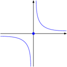
Figure 4: A total, but highly discontinuous, function.

Please observe that $\llparenthesis{\tau}\rrparenthesis^{<\infty}$ is in general a much larger set of differences than $\bigcup_{r\in\mathbb{R}_{\geq 0}^{\infty}}\llparenthesis{\tau}\rrparenthesis^{r}$: the former equals the latter only when $\tau$ is $\mathit{REAL}$. Already when $\tau$ is $\mathit{REAL}\rightarrow\mathit{REAL}$, the former includes, say, functions like $f(r,\varepsilon)=(r+\varepsilon)^{2}$, while the latter does not.

Unfortunately, there are terms in $\mathit{ST}^{\lambda}_{\mathbb{R}}$ which cannot be proved to be at self-distance in $\llparenthesis{\tau}\rrparenthesis^{<\infty}$, and, surprisingly, this is not due to the higher-order features of $\mathit{ST}^{\lambda}_{\mathbb{R}}$, but to $\{\mathcal{F}_{n}\}_{n\in\mathbb{N}}$ being arbitrary, and containing functions which do not map finite distances to finite distances, like

$$h(r)=\left\{\begin{array}[]{ll}0&\mbox{if $r=0$}\\ \frac{1}{r}&\mbox{otherwise}\end{array}\right.$$

(see Figure 4). Is this phenomenon solely responsible for the necessity of finite self-distances in $\mathit{ST}^{\lambda}_{\mathbb{R}}$? The answer is positive, and the rest of this section is devoted precisely to formalising and proving the aforementioned conjecture.

First of all, we need to appropriately axiomatise the absence of unbounded discontinuities from $\{\mathcal{F}_{n}\}_{n\in\mathbb{N}}$. A not-so-restrictive but sufficient axiom turns out to be weak boundedness: a function $f_{n}:\mathbb{R}^{n}\rightarrow\mathbb{R}$ is said to be weakly bounded if and only if it maps bounded subsets of $\mathbb{R}^{n}$ into bounded subsets of $\mathbb{R}$. As an example, the function $h$ above is not weakly bounded, because $h([-\varepsilon,\varepsilon])$ is

$$\left(-\infty,-\frac{1}{\varepsilon}\right]\cup\{0\}\cup\left[\frac{1}{\varepsilon},\infty\right)$$

which is unbounded for any as $\varepsilon>0$. Any term $M$ is said to be weakly bounded iff any function symbol $f_{n}$ occurring in $M$ is itself weakly bounded. Actually, this is precisely what one needs to get the strengthening of the Fundamental Theorem we are looking for.

Lemma 22.

Let $\cdot\vdash M,N:\tau$ and $M\Downarrow V$. Then $\delta^{\tau}({M},{N})=\delta^{\tau}({V},{N})$.

Proof.

By induction on type $\tau$; do case analysis for each type constructor. ∎

Lemma 23.

Let $\tau$ be a type and $t\in\llparenthesis{\tau}\rrparenthesis^{<\infty}$. If $t^{\prime}\leq_{\tau}t$ then $t^{\prime}\in\llparenthesis{\tau}\rrparenthesis^{<\infty}$.

Proof.

By induction on type $\tau$. Straightforward. ∎

Thoerem 24 (Fundamental Theorem, Version II).

For any weakly bounded term $\cdot\vdash M:\tau$, there is $d\in\llparenthesis{\tau}\rrparenthesis^{<\infty}$ such that $(M,d,M)\in\delta_{\tau}$.

Proof.

By induction on derivation of $\Gamma\vdash M:\tau$. In order not to make the proof too unreadable, we prove it for the case $n=1$, meaning $\Gamma=w\colon\rho$. It is straightforward (but tedious) to extend it to an arbitrarily large environment.

• Case

  $$\Gamma\vdash w:\rho w:\rho\in\Gamma.$$

  Then

  $$\begin{array}[]{ll}\delta_{\Gamma}^{\rho}({w},{w})&=\delta^{\rho\rightarrow\rho}({\lambda w.w},{\lambda w.w})\\ &=\mathop{\hbox to0.0pt{$\lambda$\hss}\mkern 2.0mu\raisebox{1.18399pt}{$\lambda$}}{\langle x^{\mathit{CV}({\rho})},y^{\llparenthesis{\rho}\rrparenthesis}\rangle}.{\sup_{z\colon\delta^{\rho}({z},{x})\leq y}\{\delta^{\rho}({(\lambda w.w)x},{(\lambda w.w)z}),\delta^{\rho}({(\lambda w.w)z},{(\lambda w.w)x})\}}\\ &=\mathop{\hbox to0.0pt{$\lambda$\hss}\mkern 2.0mu\raisebox{1.18399pt}{$\lambda$}}{\langle x^{\mathit{CV}({\rho})},y^{\llparenthesis{\rho}\rrparenthesis}\rangle}.{\sup_{z\colon\delta^{\rho}({z},{x})\leq y}\{\delta^{\rho}({x},{z}),\delta^{\rho}({z},{x})\}}\text{ by Lemma~{}\ref{lem:evalpreserve}}\\ &=\mathop{\hbox to0.0pt{$\lambda$\hss}\mkern 2.0mu\raisebox{1.18399pt}{$\lambda$}}{\langle x^{\mathit{CV}({\rho})},y^{\llparenthesis{\rho}\rrparenthesis}\rangle}.{\sup_{z\colon\delta^{\rho}({z},{x})\leq y}\delta^{\rho}({z},{x})}\text{ by Lemma~{}\ref{lem:symmetric}}\\ &\leq\mathop{\hbox to0.0pt{$\lambda$\hss}\mkern 2.0mu\raisebox{1.18399pt}{$\lambda$}}{\langle x^{\mathit{CV}({\rho})},y^{\llparenthesis{\rho}\rrparenthesis}\rangle}.{y}\in\llparenthesis{\rho\rightarrow\rho}\rrparenthesis^{<\infty}.\end{array}$$

  Hence $\delta_{\Gamma}^{\rho}({w},{w})\in\llparenthesis{\rho\rightarrow\rho}\rrparenthesis^{<\infty}$ by Lemma 23.

• Case

  $$\Gamma\vdash r:\mathit{REAL}.$$

  Easy.

• Case

  $$\Gamma\vdash f_{n}:\mathit{REAL}^{n}\rightarrow\mathit{REAL}.$$

  Straightforward.

• Case

  $$\Gamma\vdash\lambda x.M:\tau\rightarrow\rho\Gamma,x:\tau\vdash M:\rho.$$

  By induction hypothesis.

• Case

  $$\Gamma\vdash MN:\tau_{2}\lx@proof@logical@and\Gamma\vdash M:\tau_{1}\rightarrow\tau_{2}\Gamma\vdash N:\tau_{1}.$$

  Induction hypothesis in this case can be written down as:

  $$\begin{array}[]{l}\forall x_{1}\in\mathit{CV}({\rho}).\forall y_{1}\in\llparenthesis{\rho}\rrparenthesis^{<\infty}.\forall x_{2}\in\mathit{CV}({\tau_{1}}).\forall y_{2}\in\llparenthesis{\tau_{1}}\rrparenthesis^{<\infty}.\\ \sup_{z_{1}\colon\delta^{\rho}({z_{1}},{x_{1}})\leq y_{1}}\sup_{z_{2}\colon\delta^{\rho}({z_{2}},{x_{2}})\leq y_{2}}\{\delta^{\tau_{2}}({M\{x_{1}/w\}x_{2}},{M\{z_{1}/w\}z_{2}}),\delta^{\tau_{2}}({M\{x_{1}/w\}z_{2}},{M\{z_{1}/w\}x_{2}})\}\in\llparenthesis{\tau_{2}}\rrparenthesis^{<\infty}\\ \cdots\text{(I)}\end{array}$$

  $$\begin{array}[]{l}\forall x_{1}\in\mathit{CV}({\rho}).\forall y_{1}\in\llparenthesis{\rho}\rrparenthesis^{<\infty}.\\ \sup_{z_{1}\colon\delta^{\rho}({z_{1}},{x_{1}})\leq y_{1}}\delta^{\tau_{2}}({N\{x_{1}/w\}},{N\{z_{1}/w\}})\in\llparenthesis{\tau_{1}}\rrparenthesis^{<\infty}\end{array}\cdots\text{(II)}$$

  We show that $\delta_{\Gamma}^{\tau_{2}}({MN},{MN})\in\llparenthesis{\tau_{2}}\rrparenthesis^{<\infty}$, i.e. $\delta^{\tau_{2}}({\lambda w.MN},{\lambda w.MN})\in\llparenthesis{\rho\rightarrow\tau_{2}}\rrparenthesis^{<\infty}$. By definition we must show that

  $$\begin{array}[]{l}\forall x_{1}\in\mathit{CV}({\rho}).\forall y_{1}\in\llparenthesis{\rho}\rrparenthesis^{<\infty}.\\ \sup_{z\colon\delta^{\rho}({z},{x_{1}})\leq y_{1}}\{\delta^{\tau_{2}}({(\lambda w.MN)x_{1}},{(\lambda w.MN)z}),\delta^{\tau_{2}}({(\lambda w.MN)z},{(\lambda w.MN)x_{1}})\}\\ =\sup_{z\colon\delta^{\rho}({z},{x_{1}})\leq y_{1}}\delta^{\tau_{2}}({(\lambda w.MN)z},{(\lambda w.MN)x_{1}})\text{ by Lemma~{}\ref{lem:symmetric}}\\ =\sup_{z\colon\delta^{\rho}({z},{x_{1}})\leq y_{1}}\delta^{\tau_{2}}({M\{z/w\}N\{z/w\}},{M\{x_{1}/w\}N\{x_{1}/w\}})\text{ by Lemma~{}\ref{lem:evalpreserve}}\\ \in\llparenthesis{\tau_{2}}\rrparenthesis^{<\infty}.\end{array}$$

  By definition of $\sup{}$ the following inequality holds for all $x_{1}\in\mathit{CV}({\rho})$ and $y_{1}\in\llparenthesis{\rho}\rrparenthesis^{<\infty}$:

  $$\begin{array}[]{l}\sup_{z_{1}\colon\delta^{\rho}({z_{1}},{x_{1}})\leq y_{1}}\delta^{\tau_{2}}({M\{z_{1}/w\}N\{z_{1}/w\}},{M\{x_{1}/w\}N\{x_{1}/w\}})\\ \leq\sup_{z_{1}\colon\delta^{\rho}({z_{1}},{x_{1}})\leq y_{1}}\{\delta^{\tau_{2}}({M\{x_{1}/w\}N\{x_{1}/w\}},{M\{z_{1}/w\}N\{z_{1}/w\}}),\delta^{\tau_{2}}({M\{x_{1}/w\}N\{z_{1}/w\}},{M\{z_{1}/w\}N\{x_{1}/w\}})\}\\ \leq\sup_{z_{1}\colon\delta^{\rho}({z_{1}},{x_{1}})\leq y_{1}}\sup_{z_{2}\colon\delta^{\rho}({z_{1}},{N\{x_{1}/w\}})\leq s}\\ \quad\{\delta^{\tau_{2}}({M\{x_{1}/w\}N\{x_{1}/w\}},{M\{z_{1}/w\}z_{2}}),\delta^{\tau_{2}}({M\{x_{1}/w\}z_{2}},{M\{z_{1}/w\}N\{x_{1}/w\}})\},\end{array}$$

  where $s=\sup_{z_{1}\colon\delta^{\rho}({z_{1}},{x_{1}})\leq y_{1}}\delta^{\tau_{2}}({N\{x_{1}/w\}},{N\{z/w\}}).$

  Thus by Lemma 23 it suffices show that

  $$\begin{array}[]{l}\sup_{z_{1}\colon\delta^{\rho}({z_{1}},{x_{1}})\leq y_{1}}\,\sup_{z_{2}\colon\delta^{\rho}({z_{1}},{N\{x_{1}/w\}})\leq s}\\ \{\delta^{\tau_{2}}({M\{x_{1}/w\}N\{x_{1}/w\}},{M\{z_{1}/w\}z_{2}}),\delta^{\tau_{2}}({M\{x_{1}/w\}z_{2}},{M\{z_{1}/w\}N\{x_{1}/w\}})\}\in\llparenthesis{\tau_{2}}\rrparenthesis^{<\infty}.\end{array}$$

  By I.H. (I), this holds if $N\{x_{1}/w\}\in\mathit{CV}({\tau_{2}})$ and $s=\sup_{z_{1}\colon\delta^{\rho}({z_{1}},{x_{1}})\leq y_{1}}\delta^{\tau_{2}}({N\{x_{1}/w\}},{N\{z/w\}})\in\llparenthesis{\tau_{2}}\rrparenthesis^{<\infty}$; the latter holds by I.H. (II).

• Case

  $$\Gamma\vdash\langle M,N\rangle:\tau\times\rho\lx@proof@logical@and\Gamma\vdash M:\tau\Gamma\vdash N:\rho.$$

  Straightforward using induction hypothesis.

• Case

  $$\Gamma\vdash\pi_{1}:\tau\times\rho\rightarrow\tau.$$

  Straightforward.

• Case

  $$\Gamma\vdash\pi_{2}:\tau\times\rho\rightarrow\rho.$$

  Straightforward, similar to the case of $\pi_{1}$.

∎

The reader may have wondered about how restrictive a condition weak boundedness really is. In particular, whether it corresponds to some form of continuity. In fact, the introduced condition only rules out unbounded discontinuities. In other words, weak boundedness can be equivalently defined by imposing local boundedness at any point in the domain $\mathbb{R}$. This is weaker than asking for boundedness, which requires the existence of a global bound.

6 A Categorical Perspective

Up to now, differential logical relations have been treated very concretely, without looking at them through the lens of category theory. This is in contrast to, e.g., the treatment of metric relations from [11], in which soundness of metric relations for $\mathsf{FUZZ}$ is obtained as a byproduct of a proof of symmetric monoidal closedness for the category $\mathbf{MET}$ of pseudometric spaces and Lipschitz functions.

But what could take the place of pseudometric spaces in a categorical framework capturing differential logical relations? The notion of a metric needs to be relaxed along at least two axes. On the one hand, the codomain of the “metric” $\delta$ is not necessarily the set of real numbers, but a more general structure, namely a quantale. On the other, as we already noticed, it is not necessarily true that equality implies indistancy, but rather than indistancy implies inequality. What comes out of these observations is, quite naturally, the notion of a generalized metric domain, itself a generalisation of partial metrics [6]. The rest of this section is devoted to proving that the category of generalised metric domains is indeed cartesian closed, thus forming a model of simply typed $\lambda$-calculi.

Formally, given a quantale $\mathbb{Q}=(Q,\leq_{Q},0_{Q},*_{Q})$, a generalised metric domain on $\mathbb{Q}$ is a pair $(A,\delta_{A})$, where $A$ is a set and $\delta_{A}$ is a subset of $A\times\mathbb{Q}\times A$ satisfying some axioms akin to those of a metric domain:

$$\delta_{A}({x},{0_{Q}},{y}) \Rightarrow x=y;$$ (Indistancy Implies Equality)

$$\delta_{A}({x},{d},{y}) \Rightarrow\delta_{A}({y},{d},{x});$$ (Symmetry)

$$\delta_{A}({x},{d},{y})\wedge\delta_{A}({y},{e},{y})\wedge\delta_{A}({y},{f},{z}) \Rightarrow\delta_{A}({x},{d*e*f},{z}).$$ (Triangularity)

Please observe that $\delta_{A}$ is a relation rather than a function. Moreover, the first axiom is dual to the one typically found in, say, pseudometrics. The third axiom, instead, resembles the usual triangle inequality for pseudometrics, but with the crucial difference that since objects can have non-null self-distance, such a distance has to be taken into account. Requiring equality to imply indistancy (and thus $\delta_{A}({x},{0_{Q}},{y})\Leftrightarrow x=y$), we see that (Triangularity) gives exactly the usual triangle inequality (properly generalised to quantale and relations [16, 17]).

In this section we show that generalised metric domains form a cartesian closed category, unlike that of metric spaces (which is known to be non-cartesian closed). As a consequence, we obtain a firm categorical basis of differential logical relations. The category of generalised metric domain, denoted by $\mathbf{GMD}$.

Definition 25.

The category $\mathbf{GMD}$ has the following data.

• An object $\mathcal{A}$ is a triple $(A,\mathbb{Q},\delta)$ where $\mathbb{Q}$ is a quantale and $(A,\delta)$ is a generalized metric domain on $\mathbb{Q}$.

• An arrow $(A,\mathbb{Q},\delta)\to(B,\mathbb{S},\rho)$ is a pair $(f,\zeta)$ consisting of a function $f\colon A\to B$ and another function $\zeta\colon Q\times A\to S$ satisfying $\forall a,a^{\prime}\in A.\forall q\in Q.\delta(a,q,a^{\prime})\Rightarrow\rho(f(a),\zeta(q,a),f(a^{\prime}))$ and $\rho(f(a),\zeta(q,a^{\prime}),f(a^{\prime}))$.

We can indeed give $\mathbf{GMD}$ the structure of a category. In fact, the identity on the object $\mathcal{A}=(A,\mathbb{Q},\delta)$ in $\mathbf{GMD}$ is given by $(\mathrm{id}_{\mathcal{A}},\mathrm{id}_{\mathcal{A}}^{\prime})$ where $\mathrm{id}_{\mathcal{A}}\colon A\to A$ is the set-theoretic identity on $A$ and $\mathrm{id}_{\mathcal{A}}^{\prime}\colon Q\times A\to Q$ is defined by $\mathrm{id}_{\mathcal{A}}^{\prime}(q,a)=q$. The composition of two arrows $(f,\zeta)\colon(A,\mathbb{Q},\delta)\to(B,\mathbb{S},\rho)$ and $(g,\eta)\colon(B,\mathbb{S},\rho)\to(C,\mathbb{T},\nu)$ is the pair $(h,\theta)$ where $h\colon A\to C$ is given by the function composition $g\circ f\colon A\to C$ and $h\colon Q\times A\to T$ is given by $\theta(q,a)=\eta(\zeta(q,a),f(a))$. Straightforward calculations show that composition is associative, and that the identity arrow behaves as its neutral element.

Lemma 26.

$\mathbf{GMD}$ is a category.

Proof.

The identity on the object $\mathcal{A}=(A,\mathbb{Q},\delta)$ in $\mathbf{GMD}$ is given by $(\mathrm{id}_{\mathcal{A}},\mathrm{id}_{\mathcal{A}}^{\prime})$ where $\mathrm{id}_{\mathcal{A}}\colon A\to A$ is the set-theoretic ideneity on $A$ and $\mathrm{id}_{\mathcal{A}}^{\prime}\colon Q\times A\to Q$ is defined by $\mathrm{id}_{\mathcal{A}}^{\prime}(q,a)=q$. The composition of two arrows $(f,\zeta)\colon(A,\mathbb{Q},\delta)\to(B,\mathbb{S},\rho)$ and $(g,\eta)\colon(B,\mathbb{S},\rho)\to(C,\mathbb{T},\nu)$ is the pair $(h,\theta)$ where $h\colon A\to C$ is given by the function composition $g\circ f\colon A\to C$ and $h\colon Q\times A\to T$ is given by $\theta(q,a)=\eta(\zeta(q,a),f(a))$. The fact that every identity arrow and every composition are again arrows in $\mathbf{GMD}$ can be checked straightforwardly: $\mathrm{id}_{\mathcal{A}}$ clearly satisfies $\delta(a,q,a^{\prime})\Rightarrow\delta(\mathrm{id}(a),\mathrm{id}^{\prime}(q,a),\mathrm{id}(a^{\prime}))$ and $\delta(\mathrm{id}(a),\mathrm{id}^{\prime}(q,a^{\prime}),id(a^{\prime}))$ since the right-hand side is by definition $\delta(a,q,a)$. We have to check that $(h,\theta)$ satisfies $\delta(a,q,a^{\prime})\Rightarrow\nu(h(a),\theta(q,a),h(a^{\prime}))$ (and its symmetric part). Indeed, we have $\delta(f(a),\zeta(q,a),f(a^{\prime}))$ since $(f,\zeta)$ is an arrow in $\mathbf{GMD}$; and $\nu(g(f(a)),\eta(\zeta(q,a),f(a)),g(f(a^{\prime})))$, which is equivalent to $\nu(h(a),\theta(q,a),h(a^{\prime}))$ by definition, holds since $(g,\eta)$ is an arrow in $\mathbf{GMD}$. (Similarly for the symmetric part.) ∎

The construction of (finite) products in $\mathbf{GMD}$ is mostly straightforward:

Lemma 27.

The category $\mathbf{GMD}$ has a terminal object and binary products.

Proof.

The terminal object $\mathbf{GMD}$ is defined as $(\{*\},\mathbb{O},\delta_{0})$, where $\mathbb{O}$ is the one-element quantale $\{0\}$, and $\delta_{0}=\{(*,0,*)\}$. Clearly, $(\{*\},\delta_{0})$ is a generaliszed metric domain on $\mathbb{O}$ which behaves as a terminal object. Next, we show that $\mathbf{GMD}$ has binary products. Given two objects $\mathcal{A}$ and $\mathcal{B}$, their binary product $\mathcal{A}\times\mathcal{B}$ is given by a triple $(A\times B,\mathbb{Q}\times\mathbb{S},\delta\times\rho)$. The projection from $\mathcal{A}\times\mathcal{B}$ to $\mathcal{A}$ is the pair $(\pi_{1},\pi_{1}^{\prime})$ given by $\pi_{1}(a,b)=a$ and $\pi_{1}^{\prime}((q,s),(a,b))=q$ (similarly for $\pi_{2}$).

Given objects $\mathcal{A},\mathcal{B},\mathcal{C}$ and arrows $(f,\zeta)\colon\mathcal{C}\to\mathcal{A},(g,\eta)\colon\mathcal{C}\to\mathcal{B}$, the mediating arrow $\mathcal{C}\to\mathcal{A}\times\mathcal{B}$ is given by a pair $(h,\theta)$ where $h\colon C\to A\times B$ is a function $h(c)=(f(c),g(c))$ and $\theta\colon{T}\times C\to{Q}\times{S}$ is a function $\theta(t,c)=(\zeta(t,c),\eta(t,c))$. This satisfies $(\pi_{1},\pi_{1}^{\prime})\mathbin{\circ}(h,\theta)=(f,\zeta)$: on the first component, $(\pi_{1}\mathbin{\circ}h)(c)=\pi_{1}(g(c),h(c))=g(c)$. On the second, $(\pi_{1}^{\prime}\mathbin{\circ}\theta)(t,c)=\pi_{1}^{\prime}(\theta(t,c),h(c))=\pi_{1}^{\prime}((\zeta(t,c),\eta(t,c)),h(c))=\zeta(t,c)$ (similarly $(\pi_{2},\pi_{2}^{\prime})\mathbin{\circ}(h,\theta)=(g,\eta)$ holds). ∎

Lemma 28.

The category $\mathbf{GMD}$ has exponential objects.

Proof.

The exponential object $\mathcal{C}^{\mathcal{B}}$ is given by a triple $(C^{B},\mathbb{T}^{\mathbb{S}\times B},\nu^{\rho})$ where $C^{B}$ is the function space $\{f\,|\,f\colon B\to C\}$, $\mathbb{T}^{\mathbb{S}\times B}$ is the exponential quantale, and $\nu^{\rho}$ is a ternary relation over $C^{B}\times T^{S\times B}\times C^{B}$ defined by: if $\rho(b,s,b^{\prime})$ then $\nu(f(b),d(s,b),f^{\prime}(b^{\prime}))$ and $\nu(f(b),d(s,b^{\prime}),\zeta(b^{\prime}))$. The relation $\nu^{\rho}$ is indeed a differential logical relation.

Then given three objects $\mathcal{A},\mathcal{B},\mathcal{C}$ and an arrow $g\colon\mathcal{A}\times\mathcal{B}\to\mathcal{C}$, the abstraction $\lambda g\colon\mathcal{A}\to\mathcal{C}^{\mathcal{B}}$ of $g$ is given by a pair $(\lambda g,\lambda\eta)$ where $\lambda g\colon A\to C^{B}$ is defined by $\lambda g(a)(b)=g(a,b)$ and $\lambda\eta\colon{Q}\times A\to{T}^{{S}\times B}$ is defined by $\lambda\eta(q,a)(s,b)=\eta((q,s),(a,b))$.

Last, $\mathrm{eval}\colon\mathcal{C}^{\mathcal{B}}\times\mathcal{B}\to\mathcal{C}$ is given by a pair $(\mathrm{eval},\mathrm{eval}^{\prime})$ where $\mathrm{eval}\colon C^{B}\times B\to C$ is defined by $\mathrm{eval}(f,b)=f(b)$ and $\mathrm{eval}^{\prime}\colon({T}^{{S}\times B}\times{S})\times(C^{B}\times B)\to{T}$ is defined by $\mathrm{eval}^{\prime}((d,s),(f,b))=d(s,b)$.

The fact that these arrows makes the diagram

commute can be checked componentwise. Let $(h,\theta)$ be the pair comprising the composition $\mathrm{eval}\mathbin{\circ}(\lambda g\times\mathrm{id})\colon\mathcal{A}\times\mathcal{B}\to\mathcal{C}$. On the first component, we have $h((a,b))=\mathrm{eval}((\lambda g\times\mathrm{id})(a,b))=\mathrm{eval}((\lambda g(a),b))=\lambda g(a)(b)=g(a,b)$. On the second, $\theta((q,s),(a,b))=\mathrm{eval}^{\prime}((\lambda\eta\times\mathrm{id}^{\prime})(q,s)(a,b),(\lambda g\times\mathrm{id})(a,b))=\mathrm{eval}^{\prime}((\lambda\eta(q,a),\mathrm{id}^{\prime}(s,b)),(\lambda g(a),b))=\mathrm{eval}^{\prime}((\lambda\eta(q,a),s),(\lambda g(a),b))=\lambda\eta(q,a)(s,b)=\eta((q,s),(a,b))$.

∎

Joining together 27 and and 28 we obtain the wished result.

Corollary 29.

The category $\mathbf{GMD}$ is cartesian closed.

Interestingly, the constructions of product and exponential objects closely match the definition of a differential logical relation. In other words, differential logical relations as given in Definition 7 can be seen as providing a denotational model of $\mathit{ST}^{\lambda}_{\mathbb{R}}$ in which base types are interpreted by the generalised metric domain corresponding to the Euclidean distance.

7 Conclusion

In this paper, we introduced differential logical relations as a novel methodology to evaluate the “distance” between programs of higher-order calculi akin to the $\lambda$-calculus. We have been strongly inspired by some unpublished work by Westbrook and Chaudhuri [29], who were the first to realise that evaluating differences between interactive programs requires going beyond mere real numbers. We indeed borrowed our running examples from the aforementioned work.

This paper’s contribution, then consists in giving a simple definition of differential logical relations, together with some results about their underlying metatheory: two formulations of the Fundamental Lemma, a result relating differential logical relations and ordinary logical relations, a categorical framework in which generalised metric domains — the metric structure corresponding to differential logical relations — are proved to form a cartesian closed category. Such results give evidence that, besides being more expressive than metric relations, differential logical relations are somehow more canonical, naturally forming a model of simply-typed $\lambda$-calculi.

As the title of this paper suggests, we see the contributions above just as a very first step towards understanding the nature of differences in a logical environment. In particular, at least two directions deserve to be further explored.

• The first one concerns language features: admittedly, the calculus $\mathit{ST}^{\lambda}_{\mathbb{R}}$ we consider here is very poor in terms of its expressive power, lacking full higher-order recursion and thus not being universal. Moreover, $\mathit{ST}^{\lambda}_{\mathbb{R}}$ does not feature any form of effect, including probabilistic choices, in which evaluating differences between programs would be very helpful. Addressing such issues seems to require to impose a domain structure on generalised metric domain, on one hand, and to look at monads on $\mathbf{GMD}$, on the other hand (for the latter, the literature on monadic lifting for quantale-valued relations might serve as a guide [16]).

• The second one is about abstract differences: defining differences as functions with the same rank as that of the compared programs implies that reasoning about them is complex. Abstracting differences so as to facilitate differential reasoning could be the way out, given that deep connections exist between logical relations and abstract interpretation [2].

References

- [1] S. Abramsky. The lazy lambda calculus. In D. Turner, editor, Research Topics in Functional Programming, pages 65–117. Addison Wesley, 1990.
- [2] Samson Abramsky. Abstract interpretation, logical relations and Kan extensions. J. Log. Comput., 1(1):5–40, 1990.
- [3] A. Arnold and M. Nivat. Metric interpretations of infinite trees and semantics of non deterministic recursive programs. Theor. Comput. Sci., 11:181–205, 1980.
- [4] C. Baier and M.E. Majster-Cederbaum. Denotational semantics in the CPO and metric approach. Theor. Comput. Sci., 135(2):171–220, 1994.
- [5] Gilles Barthe, Marco Gaboardi, Justin Hsu, and Benjamin C. Pierce. Programming language techniques for differential privacy. SIGLOG News, 3(1):34–53, 2016.
- [6] Michael A. Bukatin, Ralph Kopperman, Steve Matthews, and Homeira Pajoohesh. Partial metric spaces. The American Mathematical Monthly, 116(8):708–718, 2009.
- [7] Konstantinos Chatzikokolakis, Daniel Gebler, Catuscia Palamidessi, and Lili Xu. Generalized bisimulation metrics. In CONCUR 2014 - Concurrency Theory - 25th International Conference, CONCUR 2014, Rome, Italy, September 2-5, 2014. Proceedings, pages 32–46, 2014.
- [8] Raphaëlle Crubillé and Ugo Dal Lago. Metric reasoning about -terms: The affine case. In Proc. of LICS 2015, pages 633–644, 2015.
- [9] Raphaëlle Crubillé and Ugo Dal Lago. Metric reasoning about -terms: The general case. In Proc. of ESOP 2017, pages 341–367, 2017.
- [10] Ugo Dal Lago, Francesco Gavazzo, and Akira Yoshimizu. Differential logical relations. Part I: The simply-typed case (extended version). 2018. URL: http://www.cs.unibo.it/~dallago/DLG.pdf.
- [11] A.A. de Amorim, M. Gaboardi, J. Hsu, S. Katsumata, and I. Cherigui. A semantic account of metric preservation. In Proc. of POPL 2017, pages 545–556, 2017.
- [12] J.W. de Bakker and J.I. Zucker. Denotational semantics of concurrency. In STOC, pages 153–158, 1982.
- [13] Josee Desharnais, Vineet Gupta, Radha Jagadeesan, and Prakash Panangaden. Metrics for labelled markov processes. Theor. Comput. Sci., 318(3):323–354, 2004.
- [14] M.H. Escardo. A metric model of pcf. In Workshop on Realizability Semantics and Applications, 1999.
- [15] Francesco Gavazzo. Quantitative behavioural reasoning for higher-order effectful programs: Applicative distances. In Proc. of LICS 2018, pages 452–461, 2018.
- [16] D. Hofmann, G.J. Seal, and W. Tholen, editors. Monoidal Topology. A Categorical Approach to Order, Metric, and Topology. Number 153 in Encyclopedia of Mathematics and its Applications. Cambridge University Press, 2014.
- [17] F.W. Lawvere. Metric spaces, generalized logic, and closed categories. Rend. Sem. Mat. Fis. Milano, 43:135–166, 1973.
- [18] John C. Mitchell. Foundations for Programming Languages. MIT Press, 1996.
- [19] Sparsh Mittal. A survey of techniques for approximate computing. ACM Comput. Surv., 48(4), 2016.
- [20] J. Morris. Lambda Calculus Models of Programming Languages. PhD thesis, MIT, 1969.
- [21] Gordon D. Plotkin. Lambda-definability and logical relations. Memorandum SAI-RM-4, University of Edinburgh, 1973.
- [22] J. Reed and B.C. Pierce. Distance makes the types grow stronger: a calculus for differential privacy. In Proc. of ICFP 2010, pages 157–168, 2010.
- [23] K.I. Rosenthal. Quantales and their applications. Pitman research notes in mathematics series. Longman Scientific & Technical, 1990.
- [24] Dana Scott. Outline of a mathematical theory of computation. Technical Report PRG02, OUCL, November 1970.
- [25] Dana Scott and Christopher Strachey. Toward a mathematical semantics for computer languages. Technical Report PRG06, OUCL, August 1971.
- [26] F. Van Breugel. An introduction to metric semantics: operational and denotational models for programming and specification languages. Theor. Comput. Sci., 258(1-2):1–98, 2001.
- [27] F. Van Breugel and J. Worrell. A behavioural pseudometric for probabilistic transition systems. Theor. Comput. Sci., 331(1):115–142, 2005.
- [28] Franck van Breugel and James Worrell. Towards quantitative verification of probabilistic transition systems. In Proc. of ICALP 2001, pages 421–432, 2001.
- [29] Edwin M. Westbrook and Swarat Chaudhuri. A semantics for approximate program transformations. CoRR, abs/1304.5531, 2013. URL: http://arxiv.org/abs/1304.5531.
- [30] Lili Xu, Konstantinos Chatzikokolakis, and Huimin Lin. Metrics for differential privacy in concurrent systems. In Proc. of FORTE 2014, pages 199–215, 2014.