Correlations between avalanches in the depinning dynamics of elastic interfaces

Abstract

We study the correlations between avalanches in the depinning dynamics of elastic interfaces driven on a random substrate. In the mean field theory (the Brownian force model), it is known that the avalanches are uncorrelated. Here we obtain a simple field theory which describes the first deviations from this uncorrelated behavior in a $\epsilon=d_{c}-d$ expansion below the upper critical dimension $d_{c}$ of the model. We apply it to calculate the correlations between (i) avalanche sizes (ii) avalanche dynamics in two successive avalanches, or more generally, in two avalanches separated by a uniform displacement $W$ of the interface. For (i) we obtain the correlations of the total sizes, of the local sizes and of the total sizes with given seeds (starting points). For (ii) we obtain the correlations of the velocities, of the durations, and of the avalanche shapes. In general we find that the avalanches are anti-correlated, the occurence of a larger avalanche making more likely the occurence of a smaller one, and vice-versa. Examining the universality of our results leads us to conjecture several new exact scaling relations for the critical exponents that characterize the different distributions of correlations. The avalanche size predictions are confronted to numerical simulations for a $d=1$ interface with short range elasticity. They are also compared to our recent related work on static avalanches (shocks). Finally we show that the naive extrapolation of our result into the thermally activated creep regime at finite temperature, predicts strong positive correlations between the forward motion events, as recently observed in numerical simulations.

I Introduction

The motion of elastic interfaces slowly driven in a random medium is not smooth but proceeds via jumps extending over a broad range of space and time scale DSFisher1998 ; SethnaDahmenMyers2001 . This avalanche motion is ubiquitous in a number of experimental systems such as magnetic domain walls ZapperiCizeauDurinStanley1998 ; DurinZapperi2000 , fluid contact lines MoulinetGuthmannRolley2002 ; LeDoussalWieseMoulinetRolley2009 , earthquakes BenZionRice1993 ; FisherDahmenRamanathanBenZion1997 , cracks Ponson2008 ; SantucciGrobToussaint2010 ; BonamySantucciPonson2008 or imbibition fronts PlanetRamonSantucci2009 , often modeled as elastic interfaces. Theoretically, the statics and the dynamics of elastic interfaces has been studied using the functional renormalization group (FRG)DSFisher1986 ; NattermannStepanowTangLeschhorn1992 ; NarayanDSFisher1992b ; NarayanDSFisher1993a ; ChauveLeDoussalWiese2000a ; LeDoussalWieseChauve2002 ; LeDoussalWieseChauve2003 ; LeDoussal2006b ; LeDoussal2008 ; MiddletonLeDoussalWiese2006 ; RossoLeDoussalWiese2006a ; RossoLeDoussalWiese2009a . The FRG has then been extended to study avalanches, either in the statics (the so-called shocks) LeDoussalWiese2008c ; LeDoussalWiese2011b , or near the depinning transition LeDoussalWiese2011a ; LeDoussalWiese2012a ; DobrinevskiLeDoussalWiese2014a ; DobrinevskiPhD ; ThieryPhD ; Tip ; ThieryShape .

An important question is to quantify the temporal and spatial correlations between successive avalanches. It is well known that in the case of earthquakes strong temporal correlations are observed, called aftershocks Omori1894 . It was believed that in the context of elastic interfaces models, correlations between avalanches arise only if one includes additional mechanisms in the interface dynamics, such as relaxation processes JaglaLandesRosso2014 ; Jagla2014 or memory effects DobrinevskiLeDoussalWiese2013 . In a recent work ThieryStaticCorrelations we have studied correlations between “static avalanches”, more precisely between the sizes and locations of the shocks in the ground state of elastic interfaces in a random potential. Although they are expected to be close cousins of the avalanches observed in the interface dynamics, they are not identical. Thus it remains to study the correlations between avalanches in the dynamics.

In this paper we study the correlations between avalanches in the depinning dynamics of elastic interfaces driven on a random substrate. The starting point is the mean-field theory, valid in space dimension $d>d_{c}$, known as the Brownian force model (BFM) LeDoussalWiese2011b ; LeDoussalWiese2011a ; LeDoussalWiese2012a ; ThieryLeDoussalWiese2015 ; Delorme a multidimensional generalization of the celebrated ABBM model AlessandroBeatriceBertottiMontorsi1990 . In the BFM, the avalanches are strictly uncorrelated ThieryLeDoussalWiese2015 . Here we obtain a simple field theory, based on the FRG, which describes the first deviations from this uncorrelated behavior in a $\epsilon=d_{c}-d$ expansion below the upper critical dimension of the model (which depends on the range of the elastic interaction, $d_{c}=4$ for short-range (SR) elasticity and $d_{c}=2$ for usual long-range (LR) elasticity). The elastic model and the avalanche observables are defined in Section II. The field theory is described in III and Appendix C, together with a discussion of the physical origin of the correlations.

We apply our theory to calculate the correlations of two successive avalanches, loosely meaning two avalanches which occur within the same dynamical forward evolution of the interface in a given pinning landscape. It is convenient to study two avalanches separated by a given displacement $W$ of the center of mass of the interface. For $W=0^{+}$ this describes immediately successive avalanches. We study two types of information, (i) the correlations of the avalanche sizes, in Section IV, and (ii) the correlations in the dynamics within each avalanche, in Section VI. More precisely for (i) we obtain the correlation between the total sizes, the local sizes, and the total size of avalanches with given seeds (i.e. given position of their starting points). We show that the first two results are equal to this order in the expansion, i.e. to $O(\epsilon)$, to the ones obtained in the statics ThieryStaticCorrelations for random field disorder (differences are expected to the next order). These results are derived here in a much simpler fashion. The third one, the correlation of the total size as the distance between the seeds is varied, is new. Some of these analytical predictions are confronted, in Section V, to numerical simulations for a $d=1$ interface with short range elasticity. For the dynamics (ii) we obtain the correlations of the velocities, of the avalanche durations, and of the avalanche shapes, i.e. of the velocity as a function of time at fixed duration. For the latter, a deviation from the famous parabola shape is demonstrated in the correlation. Examining the universal limit of our results, we obtain some new non-trivial (and presumably exact, i.e. valid beyond the $\epsilon$ expansion) conjectures for a variety of critical exponents that characterize the correlations.

We find that in the depinning dynamics the avalanches are anti-correlated, the occurence of a larger avalanche (in size, in total velocity etc..) making more likely the occurence of a smaller one, and vice-versa. The same was observed in the statics (i.e for correlations between shocks) for random field disorder, while both positive and negative correlations could occur for random bond disorder depending on $W$. In the conclusion we discuss qualitatively some possible extension at finite temperature which indicates instead the occurence of positive correlations in the creep regime.

II Model and observables

II.1 Model

We focus on a $d$-dimensional elastic interface whose position at point $x\in{\mathbb{R}}^{d}$ and time $t\in{\mathbb{R}}$, $u(x,t)\in{\mathbb{R}}$, satisfies the following equation of motion

$$\eta\partial_{t}u(x,t)=\nabla^{2}_{x}u(x,t)-m^{2}(u(x,t)-w(x,t))+F(u(x,t),x)\,.$$ (1)

The random pinning force $F(u,x)$ is chosen Gaussian with correlator

$$\overline{F(u,x)F(u^{\prime},x^{\prime})}=\delta^{d}(x-x^{\prime})\Delta_{b}(u-u^{\prime})\,.$$ (2)

where $\Delta_{b}(u)$ denotes the bare correlator, assumed to be a symmetric short-range function. Here we have restricted to elastic interfaces with short-range elasticity and the elastic coefficient (coefficient in front of the Laplacian in (1)) has been set to unity by a choice of units. The interface is driven by a parabolic well of stiffness $m^{2}$ following some driving protocol $w(x,t)$. We restrict to monotonous driving $\dot{w}(x,t)\geq 0$ which leads to only forward motion $\dot{u}(x,t)\geq 0$ and to the so-called Middleton attractor. The lateral extension of the interface is noted $L>0$ and we assume periodic boundary conditions, although this will be unimportant as long as $L\gg 1/m$, the scale over which the interface motion is correlated. Our theory extends to other types of elasticity and more general microscopic disorder as in ThieryStaticCorrelations but here we focus on this setting for the sake of simplicity.

Our aim is to study the avalanches that occur in the so-called quasistatic limit. There are two main protocols that are largely equivalent.

1. In the first protocol the interface driving is $w(x,t)=vt$ and we are interested in the stationary state middleton1992asymptotic in the limit $v=0^{+}$ where the motion of the interface is intermittent. The avalanches are defined by the rapid motion $\dot{u}(x,t)\gg v$ that occur in between quiescence periods (of duration of order $1/(L^{d}v)$).The avalanches can be indexed by the time at which they occur and their starting point ($x_{i},t_{i}$) and we can ask about the correlations of these avalanches. Equivalently the process $u(x;w)=\lim_{v\to 0}u(x,t=w/v)$ exhibits jumps as a function of $w$ that are the avalanches. This process is called the quasi-static process and our goal is to study correlations between different given avalanches as a function of $W$, the distance along $u$ between two given avalanches, or equivalently ${\sf T}=W/v$, the time interval between the two avalanches (see Fig. 1). Note that for $W>0$ many other avalanches have usually occured between the two avalanches under study.

2. In the second protocol we prepare the system in the same stationary state, stop the driving at $w=0$ and wait for the interface to stop. It is thereby prepared with $\dot{u}(x,t=0)=0$ in the so-called Middleton attractor middleton1992asymptotic . Then we apply a kick at $t=0$, $\dot{w}(x,t)=\delta w(x)\delta(t)$, either (i) local $\delta w(x)=\delta w\,\delta^{d}(x)$ or (ii) uniform $\delta w(x)=\delta w$. This produces some interface motion, that we call an avalanche. Choosing uniform kicks of vanishing size $\delta w$ ensures that the interface stops at the position $u(x;\delta w)$ previously defined in the first protocol in the limit $v\to 0^{+}$. To study the correlation between avalanches, we apply a series of such kicks, waiting each time for the interface to stop before applying the next kick. After $n\gg 1$ kicks the driving is now at $w=n\delta w$ and the position of the interface is $u(x;w)$.

For the sake of simplicity we use in this paper the language of the second protocol and more often consider uniform kicks (although the dependence in the positions of the avalanche starting points, the seeds, will be investigated using a local kick, see below). We derive results using the functional renormalization group and these will be accurate and universal in the limit of small $m$ (with still $L\gg 1/m$), in an expansion in $\epsilon=4-d$ around the upper-critical dimension $d_{\rm uc}=4$ of the model. We thus restrict ourselves to $d<4$, although equivalent results for $d=4$ could be obtained.

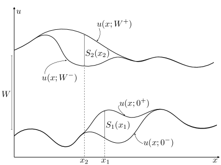
Figure 1: The quasistatic process $u(x;w)$ for an elastic interface slowly driven in a disordered environment exhibits jumps called avalanches as a function of $w$ (the position of the driving well). Here an avalanche occured at $w=0$ and another one at $w=W$ (many others also occured in between since $u(x;0^{+})\neq u(x,W^{-})$). The goal of this article is to study the correlations between these two avalanches. In particular the correlations between the total jumps (the areas of the two avalanches) or between the local jumps $S_{1}(x_{1})$ and $S_{2}(x_{2})$ indicated on the figure.

II.2 Observables

We focus on the correlations between two avalanches, the first occuring after a uniform kick of size $\delta w_{1}$ at $w=0$ and the second occuring after a uniform kick of size $\delta w_{2}$ at $w=W$. If $W>0$ potentially many avalanches have also occured in between. We start by considering the full velocity field inside an avalanche. It is convenient to adopt the following representation. We define two copies of the velocity field shifted in time $\dot{u}_{1}(x,\tau_{1})$ and $\dot{u}_{2}(x,\tau_{2})$ where $\tau_{1}$ and $\tau_{2}$ denote the time since the beginning of respectively the first and second avalanche (i.e. the first and the second kick, recalling that, according to the second protocol described above there has been many kicks in between to move the interface from $w=0$ to $w=W$).

II.2.1 Velocity fields during avalanches and their associated densities

We consider a general observable of the form (i.e. the generating function of the velocity field)

$$G[\lambda]=\overline{e^{\int d^{d}xdt\lambda(x,t)\dot{u}(x,t)}}\,.$$ (3)

Decomposing the source field $\lambda(x,t)$ as done above for the velocity, this can be rewritten

$$G[\lambda]=G[\lambda_{1},\lambda_{2}]=\overline{e^{\lambda_{1}\cdot\dot{u}_{1}+\lambda_{2}\cdot\dot{u}_{2}}}\,,$$ (4)

where here and below we denote for each $i=1,2$

$$\lambda_{i}\cdot\dot{u}_{i}=\int d^{d}x\int_{0}^{+\infty}d\tau_{i}\lambda_{i}(x,\tau_{i})\dot{u}_{i}(x,\tau_{i})\,,$$ (5)

where the source field $\lambda_{1}$ (respectively $\lambda_{2}$) is only non vanishing in the first (respectively the second) avalanche.

The generating function $G[\lambda]$ depends on the size of the kicks $\delta w_{i}$ and can be expanded as follows

$$G[\lambda_{1},\lambda_{2}]=1+\sum_{i=1,2}\delta w_{i}\int D\dot{u}_{i}\rho[\dot{u}_{i}](e^{\lambda_{i}\cdot\dot{u}_{i}}-1)+\delta w_{1}\delta w_{2}\int D[\dot{u}_{1},\dot{u}_{2}]\rho_{W}[\dot{u}_{1},\dot{u}_{2}](e^{\lambda_{1}\cdot\dot{u}_{1}}-1)(e^{\lambda_{2}\cdot\dot{u}_{2}}-1)+O(\delta w_{1}^{2},\delta w_{2}^{2})\,.$$ (6)

This is obtained by decomposing the process into events where either an avalanche occurs $\dot{u}>0$ or does not occur $\dot{u}=0$ . The terms of order $\delta w_{i}$ account for the contribution to $G$ coming from events where an avalanche occured at $w=0$ or $w=W$, while the term of order $\delta w_{1}\delta w_{2}$ accound for the contribution to $G$ where avalanches occured at both positions. Here the factors $\rho[\dot{u}_{i}]$ denote the (equal by stationarity of the protocol considered here) functional densities of the instantaneous velocity field taking the configuration $\dot{u}_{i}(x,\tau)$ during the corresponding avalanche (and $\int D\dot{u}_{i}$ denotes a functional integral). It is normalized as $\int D\dot{u}_{i}\rho[\dot{u}_{i}]=\rho_{0}$ where $\rho_{0}\sim L^{d}$ is the total density of avalanches per unit of driving $\delta w$. Similarly $\rho_{W}[\dot{u}_{1},\dot{u}_{2}]$ is the joint density, i.e it is proportional to the number of events where two avalanches occured at $w=0$ and $w=W$ with velocity fields $\dot{u}_{i}(x,\tau)$. A more detailed discussion of the formula (6) is given in Appendix B. If avalanches were independent, as is the case for the mean-field BFM (where they form a Levy jump process LeDoussalWiese2011b ; ThieryLeDoussalWiese2015 ) one would have $\rho_{W}[\dot{u}_{1},\dot{u}_{2}]=\rho[\dot{u}_{1}]\rho[\dot{u}_{2}]$. The present theory goes beyond the independent avalanche process, and allows to compute the connected joint density

$$\rho^{c}_{W}[\dot{u}_{1},\dot{u}_{2}]=\rho_{W}[\dot{u}_{1},\dot{u}_{2}]-\rho[\dot{u}_{1}]\rho[\dot{u}_{2}]\,,$$ (7)

which vanishes in the mean field theory.

II.2.2 Total and local avalanche size

The theory presented in this paper allows to study any correlation between the two velocity fields in the two avalanches. In this paper, to make calculations and results explicit, we will first focus on the total and local size of the two avalanches (the velocities being studied later in Section VI). The local size of avalanche $i=1,2$ is defined as the total displacement of the interface at a given point (see Fig. 1)

$$S_{i}(x):=\int_{0}^{+\infty}d\tau_{i}\dot{u}_{i}(x,\tau_{i})\,,$$ (8)

and the total size is given by

$$S_{i}=\int d^{d}xS_{i}(x)\,,$$ (9)

that is the area spanned by the avalanche.

The densities for these quantities can be obtained by considering the generating function (4) for source fields chosen as $\lambda_{i}(x,\tau)=\lambda_{i}$, for the total size, and as $\lambda_{i}(x,\tau)=\lambda_{i}\delta^{d}(x-x_{i})$ for the local sizes $S(x_{i})$. Expanding in powers of $\delta w_{i}$ gives, for the total size

$$G[\lambda_{1},\lambda_{2}]=1+\sum_{i=1,2}\delta w_{i}\int_{0}^{+\infty}dS_{i}\rho(S_{i})(e^{\lambda_{i}S_{i}}-1)$$ (10)

$$+\delta w_{1}\delta w_{2}\int_{0}^{+\infty}dS_{1}\int_{0}^{+\infty}dS_{2}\rho_{W}(S_{1},S_{2})(e^{\lambda_{1}S_{1}}-1)(e^{\lambda_{2}S_{2}}-1)+O(\delta w_{1}^{2},\delta w_{2}^{2})\,,$$ (11)

where $\rho(S)$ is the single avalanche total size density (per unit $w$) normalized as $\int_{0}^{+\infty}dSS\rho(S)=1$ and $\rho_{W}(S_{1},S_{2})$ is the joint density of the total sizes $S_{1},S_{2}$ in the two avalanches. We also define the connected joint density as

$$\rho^{c}_{W}(S_{1},S_{2})=\rho_{W}(S_{1},S_{2})-\rho(S_{1})\rho(S_{2})\,,$$ (12)

which vanishes in mean field theory (the BFM) and, as we show below, is $O(\epsilon)$ where $\epsilon=d_{c}-d$, near the upper critical dimension $d_{c}=4$. Similarly, for the local size we have the same expansion (10) with $S_{i}\to S_{i}(x_{i})$ and the corresponding densities $\rho(S_{i}(x_{i}))$ and $\rho_{W}(S_{1}(x_{1}),S_{2}(x_{2}))$. In Sec. IV.3 we will also study the total size of avalanches conditioned on starting at a given point. The associated densities are defined in the same way.

III Dynamical field theory for velocity field correlations in two avalanches

We now present the dynamical field theory which allows us to calculate the densities previously introduced to leading order in the $\epsilon=d_{c}-d$ expansion. We also comment on the physical origin of the correlations.

III.1 Field theory

We now go back to consider the generating function $G[\lambda_{1},\lambda_{2}]$ in (4) for general sources. Our main result, justified in Appendix C, is that, to lowest order in an expansion around mean-field (i.e. independent avalanches), the generating function which only measures the dynamics during the two avalanches separated by $W$ (see introduction) can be written as as the a functional average

$$G[\lambda_{1},\lambda_{2}]=\int D[\tilde{u}_{1},\dot{u}_{1},\tilde{u}_{2},\dot{u}_{2}]e^{\sum_{i=1,2}[\lambda_{i}\cdot\dot{u}_{i}+m^{2}\delta w_{i}\int d^{d}x\tilde{u}_{i}(x,\tau_{i}=0)]-S[\tilde{u}_{1},\dot{u}_{1},\tilde{u}_{2},\dot{u}_{2}]}\,,$$ (13)

over the following dynamical action

$$S[\tilde{u}_{1},\dot{u}_{1},\tilde{u}_{2},\dot{u}_{2}]=S_{BFM}[\tilde{u}_{1},\dot{u}_{1}]+S_{BFM}[\tilde{u}_{2},\dot{u}_{2}]+\Delta^{\prime\prime}(W)\int d^{d}x\int_{\tau_{1},\tau_{2}>0}\tilde{u}_{1}(x,\tau_{1})\tilde{u}_{2}(x,\tau_{2})\dot{u}_{1}(x,\tau_{1})\dot{u}_{2}(x,\tau_{1})\,.$$ (14)

Here $S_{\rm BFM}$ is the dynamical action associated to the BFM model

$$S_{\rm BFM}[\dot{u},\tilde{u}]=\int d^{d}x\left[\int_{\tau>0}\tilde{u}(x,\tau)(\eta\partial_{\tau}-\nabla^{2}+m^{2})\dot{u}(x,\tau)-\sigma\int_{\tau>0}\tilde{u}(x,\tau)^{2}\dot{u}(x,\tau)\right]\,,$$ (15)

following a uniform kick $\delta w$ at time $\tau=0$. Here $\sigma=-\Delta^{\prime}(0^{+})>0$ and here and below $\Delta(w)$ denotes the renormalized disorder correlator defined from the two point corrrelation function of the position of the center of mass, $u(w)=L^{-d}\int d^{d}xu(x,t=w/v)$, as

$$\Delta(w-w^{\prime})=m^{4}L^{d}\overline{(u(w)-w)(u(w^{\prime})-w^{\prime})}^{c}\,,$$ (16)

which is implicitly a function of $m$ and reproduces the bare disorder correlator in the limit of large $m$, i.e. $\Delta_{b}(w)=\lim_{m\to+\infty}\Delta(w)$. Here we focus on the universal $m\to 0$ limit, where $\Delta(w)$ has been shown LeDoussalWieseChauve2002 ; RossoLeDoussalWiese2006a to take the scaling form

$$\Delta(w)=A_{d}m^{\epsilon-2\zeta}\tilde{\Delta}(wm^{\zeta})\quad,\quad A_{d=4}=8\pi^{2}\quad,\quad\tilde{\Delta}^{*\prime\prime}(0^{+})=\frac{1-\zeta_{1}}{3}\epsilon+O(\epsilon^{2})$$ (17)

with $A_{d}=2^{d-1}\pi^{d/2}/\Gamma(3-\frac{d}{2})$. Here $\tilde{\Delta}(w)$ converges as $m\to 0$ to the FRG fixed point $\tilde{\Delta}^{*}(w)$, which is uniformly of order $O(\epsilon)$ and solution of the FRG fixed point equation, where $\zeta=\zeta_{1}\epsilon+O(\epsilon^{2})$ is the roughness exponent, with $\zeta_{1}=1/3$ for interface depinning. Note that the depinning fixed point has one undetermined, non-universal constant $\kappa$, i.e. one can write $\tilde{\Delta}^{*}(w)=\kappa^{2}\Delta^{*}(w/\kappa)$, however $\tilde{\Delta}^{*\prime\prime}(0^{+})$ is fully universal, given in (17). The corresponding form for long-range elasticity can be found in ThieryStaticCorrelations . To lowest order in $\epsilon$ the model is thus equivalent to two BFM models with a single inclusion (at some fixed $\tau_{1},\tau_{2}$) of the vertex $\Delta^{\prime\prime}(W)$ in (14) (see also (III.2) below, the result being later summed over all $\tau_{1},\tau_{2}$). Diagrammatically it is represented by two trees (the two BFM’s) joined (i.e. correlated) by a single vertex $\Delta^{\prime\prime}(W)$, as in Fig. 106 of ThieryStaticCorrelations (the same diagram holds for the dynamics, with time running upward).

The above theory allows to calculate exactly the correlations of the velocity field at order $O(\delta w_{1}\delta w_{2})$ and to order $O(\epsilon)$ in the stationary setting defined in the introduction. Expanding Eq. (13) in powers of $\delta w_{1},\delta w_{2}$ and comparing with Eq. (6), identifying the terms, we obtain the Laplace transform of the single avalanche velocity field density in terms of the correlation of the response field as

$$\int D\dot{u}_{1}\rho[\dot{u}_{1}][e^{\lambda_{1}\cdot\dot{u}_{1}}-1]=m^{2}\int D[\tilde{u}_{1},\dot{u}_{1}]\int dx\tilde{u}_{1}(x,0)e^{\lambda_{1}\cdot\dot{u}_{1}-S_{\rm BFM}[\tilde{u}_{1},\dot{u}_{1}]}\,,$$ (18)

as well as the joint density of velocity fields in the two avalanches, as

$$\int D[\dot{u}_{1},\dot{u}_{2}]\rho_{W}[\dot{u}_{1},\dot{u}_{2}](e^{\lambda_{1}\cdot\dot{u}_{1}}-1)(e^{\lambda_{2}\cdot\dot{u}_{2}}-1)$$ (19)

$$=m^{4}\int D[\tilde{u}_{1},\dot{u}_{1},\tilde{u}_{2},\dot{u}_{2}]\int dx_{1}\tilde{u}_{1}(x_{1},0)\int dx_{2}\tilde{u}_{2}(x_{2},0)e^{\sum_{i=1,2}\lambda_{i}\cdot\dot{u}_{i}-S[\tilde{u}_{1},\dot{u}_{1},\tilde{u}_{2},\dot{u}_{2}]}\,.$$

We now make these results more explicit by focusing on simpler observables, namely the joint densities and correlations of the total sizes $S_{1},S_{2}$, as well as the local sizes $S_{1}(x),S_{2}(y)$ of the two avalanches.

Remark 1: To be more precise, we stress that the above theory is devised to calculate the $O(\epsilon)$ result for the connected correlations between two avalanches. For the velocity field statistics inside a single avalanche it only leads to the mean field result, i.e. $O(\epsilon^{0})$. To obtain the $O(\epsilon)$ correction to the latter one needs to add other terms (involving $\Delta^{\prime\prime}(0)$) in the action as was done in LeDoussalWiese2012a (see also Appendix C). This is not our purpose here, and one should remember that only the results that we obtain for the connected correlations (the sole purpose of this paper) between avalanches are exact up to order $O(\epsilon)$.

Remark 2: The above setup and results can be easily generalized to study correlations between avalanches that are conditioned on starting at any given position (called the ‘seed’) along the interface. Replacing $\int dx_{1}\tilde{u}_{1}(x_{1},0)\int dx_{2}\tilde{u}_{2}(x_{2},0)\to\tilde{u}_{1}(x_{1},0)\tilde{u}_{2}(x_{2},0)$ in (19) for given $x_{1}$ and $x_{2}$ fixed, indeed selects the avalanches that have started at $x=x_{1}$ at $w=0$ and at $x=x_{2}$ at $w=W$. The easiest way to see this is to slightly modify our protocol by triggering the avalanches at $w=0$ and $w=W$ by local kicks $\delta w_{i}(x)=\delta^{d}(x-x_{i})\delta w_{i}$ of vanishing size $\delta w_{i}$. Such kicks can indeed only trigger avalanches with seeds $x_{1}$ and $x_{2}$. One then easily generalizes (10) to this case, see also Appendix B. This is used in Sec. IV.3. We refer the reader to ThieryShape ; ThieryPhD for more details about this seed centering procedure in the field theory.

Remark 3: One can study truly successive avalanches by simply considering the limit $W=0^{+}$. The present theory applies as long as the second avalanche starts well after the first one is finished. It would be interesting to study overlapping avalanches, but this goes beyond this paper (see discussion in Appendix B).

III.2 Origin of correlations

Before we go further here let us comment here on the physical origin of the correlations. The correlations originate from the fact that the time derivatives of the pinning forces $\partial_{\tau_{i}}F(u_{i}(x,\tau_{i}))$, which enters the equation of motion for the velocity, are correlated, their covariance being

$$\overline{\partial_{\tau_{1}}F(u_{1}(x,\tau_{1}),x)\partial_{\tau_{2}}F(u_{2}(x^{\prime},\tau_{2}),x^{\prime})} = \partial_{\tau_{1}}\partial_{\tau_{2}}\Delta(u_{1}(x,\tau_{1})-u_{2}(x,\tau_{2})+W)\delta^{d}(x-x^{\prime})$$

$$\simeq -\dot{u}_{1}(x,\tau_{1})\dot{u}_{2}(x,\tau_{2})\Delta^{\prime\prime}(W)\delta^{d}(x-x^{\prime})$$

This is because two displacement fields in the two avalanches see the same static random pinning force landscape. This landscape is correlated in the direction of the motion, and the correlation, at fixed value of $u_{1}(x,\tau_{1})-u_{2}(x,\tau_{2})$ extend to arbitrary time difference (we recall that $\tau_{i}$ are counted from the beginning times ${\sf T}_{i}$ of each avalanche, e.g. hence $u_{i}(x,\tau_{i})=u(x,t={\sf T}_{i}+\tau_{i})$, where ${\sf T}_{2}-{\sf T}_{1}\sim W/v$ is a very large time).

One could object, however, that the SR correlator of the bare (i.e. microscopic) model, $\Delta_{b}(w)$, has correlations only on short distance $w\sim r_{f}$, leading to correlations of the displacements only within the (small and fixed) Larkin volume. However, the renormalized correlator, $\Delta(w)$, which includes the effect of the interplay of elasticity and disorder at all scales is correlated on the much larger distance $w\sim m^{-\zeta}$. It is this renormalized correlator that must be used here. It is possible to prove this fact (and also justify that it is $\sigma=-\Delta^{\prime}(0^{+})$ which must be used in the BFM) by consideration of the effective action of the theory. Some steps in that direction are provided in the Appendix C. Physically, correlations live on the scale $w\sim m^{-\zeta}$ because this is the scale of the displacement of the interface during avalanches. In the dynamics we always find that the correlations are negative. It can be seen already from the negative correlation of the forces in (III.2) (since $\Delta^{\prime\prime}(W)>0$ near the depinning fixed point and the velocities are positive). One finds that if one avalanche occured and the interface moved on a distance $m^{-\zeta}$, the driving has to ‘catch up’ with this scale $w\sim m^{-\zeta}$ in order for the interface to forget that this avalanche has already occured.

IV Analytical results: Correlations of the avalanche sizes, total and local

IV.1 Joint density of total sizes

We first consider the total sizes of the avalanches defined in (9).

IV.1.1 Expressions for Laplace tranform

Following the same steps as in the previous section, expanding (13) in powers of $\delta w_{1},\delta w_{2}$ in the special case of constant sources $\lambda_{i}(x,\tau)=\lambda_{i}$ and comparing with (10) we obtain the Laplace transform of $\rho(S)$ as

$$\int dS_{1}\rho(S_{1})[e^{\lambda_{1}S_{1}}-1]=m^{2}\int D\tilde{u}_{1}D\dot{u}_{1}\int dx\tilde{u}_{1}(x,0)e^{\lambda_{1}\int dx\int_{0}^{+\infty}d\tau_{1}\dot{u}_{1}(x,\tau_{1})-S_{BFM}[\tilde{u}_{1},\dot{u}_{1}]}\,,$$ (21)

a formula similar to (18), and the Laplace transform of $\rho_{W}(S_{1},S_{2})$ as

$$\int dS_{1}dS_{2}\rho_{W}(S_{1},S_{2})[e^{\lambda_{1}S_{1}}-1][e^{\lambda_{2}S_{2}}-1]$$ (22)

$$=m^{4}\int D\tilde{u}_{1}D\dot{u}_{1}\int D\tilde{u}_{2}D\dot{u}_{2}\int dx_{1}\tilde{u}_{1}(x_{1},0)\int dx_{2}\tilde{u}_{2}(x_{2},0)e^{\sum_{i=1,2}\lambda_{i}\int d^{d}x\int_{0}^{+\infty}d\tau_{i}\dot{u}_{i}(x,\tau_{i})-S[\tilde{u}_{1},\dot{u}_{1},\tilde{u}_{2},\dot{u}_{2}]}\,,$$

a formula similar to (19). We now compute explicity the r.h.s. of these equations.

IV.1.2 Review of the calculation of $\rho(S)$

The r.h.s of (21) can be obtained from a standard calculation within the BFM. The main observation is that the field $\dot{u}_{1}$ in the exponential on the r.h.s. of (21) appears only linearly LeDoussalWiese2012a . Hence integrating over it leads to a delta function which constrains $\tilde{u}(x,t)$ to be a solution of the so-called instanton equation equation LeDoussalWiese2012a , in the present case given by

$$\tilde{u}(x,t)=\tilde{u}\quad,\quad-m^{2}\tilde{u}+\sigma\tilde{u}^{2}=-\lambda\,,$$ (23)

which is

$$\tilde{u}=\frac{1}{m^{2}S_{m}}Z(\lambda S_{m})\quad,\quad Z(\lambda)=\frac{1}{2}(1-\sqrt{1-4\lambda})\,,$$ (24)

where $S_{m}=\frac{\sigma}{m^{4}}$ is the typical scale of the largest avalanches in the BFM. This leads to

$$\int dS_{1}\rho(S_{1})[e^{\lambda_{1}S_{1}}-1]=\frac{1}{S_{m}}L^{d}Z(S_{m}\lambda)\,,$$ (25)

which leads to the total size density

$$\rho(S)=\frac{L^{d}}{S_{m}^{2}}\hat{\rho}(S/S_{m})\quad,\quad\hat{\rho}(s)=\frac{1}{2\sqrt{\pi}s^{3/2}}e^{-s/4}\,,$$ (26)

which is the classic result for the BFM (exact in our setting at order $O(\epsilon^{0})$). Note that $\int_{0}^{+\infty}dss\hat{\rho}(s)=1$ and $\int_{0}^{+\infty}dss^{2}\hat{\rho}(s)=2$.

IV.1.3 Calculation of $\rho_{W}(S_{1},S_{2})$

The r.h.s of (22) can be obtained from a modification of the previous calculation. The difficulty is the term proportional to $\Delta^{\prime\prime}(W)\dot{u}_{1}\dot{u}_{2}$ in the action $S$ in Eq. (14). It can be decoupled by the following calculational trick. We introduce formal centered Gaussian noise fields $\xi_{i}(x,t)$ as

$$e^{-\Delta^{\prime\prime}(W)\int d^{d}x\int_{\tau_{1},\tau_{2}>0}\tilde{u}_{1}(x,\tau_{1})\tilde{u}_{2}(x,\tau_{2})\dot{u}_{1}(x,\tau_{1})\dot{u}_{2}(x,\tau_{1})}=\langle e^{\sum_{i=1,2}\int d^{d}x\int_{0}^{+\infty}d\tau_{i}\xi_{i}(x)\tilde{u}_{i}(x,\tau_{i})\dot{u}_{i}(x,\tau_{i})}\rangle_{\xi}\,,$$ (27)

where by definition

$$\langle\xi_{i}(x)\xi_{j}(x^{\prime})\rangle_{\xi}=-(1-\delta_{ij})\Delta^{\prime\prime}(W)\delta^{d}(x-x^{\prime})\,.$$ (28)

For a given noise $\xi_{i}(x)$, the velocity fields now appear linearly and one can integrated over them (as in the BFM). This, for each realization of the noise $\xi$, constrains the response fields $\tilde{u}_{i}(x,t)$ to obey two decoupled instanton equations, whose solutions are time independent but space inhomogeneous, $\tilde{u}_{i}(x,t)=\tilde{u}_{i}(x)$, where $\tilde{u}_{i}(x)$ for $i=1,2$ are solution of

$$(\nabla_{x}^{2}-m^{2})\tilde{u}_{i}(x)+\sigma\tilde{u}_{i}(x)^{2}=-\xi_{i}(x)\tilde{u}_{i}(x)-\lambda_{i}\,.$$ (29)

The solutions of these equations are coupled because the noises $\xi_{1}$ and $\xi_{2}$ are not independent, and correlated as in (28). From these solutions, and from (22), one obtains the Laplace transform of the joint density as

$$\int dS_{1}dS_{2}\rho_{W}(S_{1},S_{2})[e^{\lambda_{1}S_{1}}-1][e^{\lambda_{2}S_{2}}-1]=m^{4}\int d^{d}x_{1}\int d^{d}x_{2}\langle\tilde{u}_{1}(x_{1})\tilde{u}_{2}(x_{2})\rangle_{\xi}\,.$$ (30)

Being interested in computing $\rho_{W}(S_{1},S_{2})$ in first order in $\Delta^{\prime\prime}(W)$ (which is itself $O(\epsilon)$) implies that we only need to solve perturbatively (29) to first order in $\xi$. To this order the solutions can be written as

$$\tilde{u}_{i}(x)=\tilde{u}^{0}_{i}+\tilde{u}^{1}_{i}(x)\quad,\quad\tilde{u}^{0}_{i}=\frac{1}{m^{2}S_{m}}Z(S_{m}\lambda_{i})\,,$$ (31)

and in Fourier space

$$\tilde{u}^{1}_{i}(q)=\frac{1}{m^{2}S_{m}}\,\frac{Z(S_{m}\lambda_{i})}{q^{2}+m^{2}-2m^{2}Z(S_{m}\lambda_{i})}\xi_{i}(q)\,.$$ (32)

Leading to our main result for the connected joint density

$$\int dS_{1}dS_{2}\rho^{c}_{W}(S_{1},S_{2})[e^{\lambda_{1}S_{1}}-1][e^{\lambda_{2}S_{2}}-1]=-\Delta^{\prime\prime}(W)\frac{L^{d}}{m^{4}S_{m}^{2}}\,\frac{Z(S_{m}\lambda_{1})}{1-2Z(S_{m}\lambda_{1})}\,\frac{Z(S_{m}\lambda_{2})}{1-2Z(S_{m}\lambda_{2})}\,,$$ (33)

where the part proportional to $\tilde{u}_{1}^{0}\tilde{u}_{2}^{0}$ cancels in the connected density.

The formula (33) if formally identical to the result Eq. (71) in ThieryStaticCorrelations for the statics. This shows that the present theory reproduces the results of (33) in a much simpler fashion. However, one must stress that the renormalized correlator $\Delta(W)$ is different in the dynamics from its value e.g. for random bond statics, leading to a numerically different result.

By expanding (33) in powers of $\lambda_{i}$ one obtains the integer moments over $\rho^{c}_{W}$ which we denote $\langle\dots\rangle_{W}^{c}$. Similarly the averages over the single avalanche density $\rho$ are denoted as $\langle\cdots\rangle$ . We give here two explicit formula, which are tested in the numerics in Sec. V below. First one finds

$$\frac{\langle S_{1}S_{2}\rangle_{W}^{c}}{\langle S\rangle^{2}}=-\frac{\Delta^{\prime\prime}(W)}{m^{4}L^{d}}\,,$$ (34)

which is in fact an exact result, and can be seen to follow from the definition (16) of the renormalized disorder correlator. The proof is identical to the statics case, to which we refer (Eq. (8) and Section III.F. and IV. E. in ThieryStaticCorrelations ). Another result is

$$\frac{\langle S_{1}^{2}S_{2}\rangle_{W}^{c}}{\langle S^{2}\rangle\langle S\rangle}=\frac{\langle S_{1}S_{2}^{2}\rangle_{W}^{c}}{\langle S^{2}\rangle\langle S\rangle}=-3\frac{\Delta^{\prime\prime}(W)}{m^{4}L^{d}}\,,$$ (35)

which holds only to order $O(\epsilon)$. Note that to the order that we calculate here $\langle S_{1}^{2}S_{2}\rangle_{W}^{c}=\langle S_{1}S_{2}^{2}\rangle_{W}^{c}$ and more generally, at this order the correlation between the two avalanches are symmetric (which is likely not to hold to higher orders in the $\epsilon$ expansion contrary to the statics).

As in ThieryStaticCorrelations , (33) can be inverse Laplace transformed, and leads to the complete $O(\epsilon)$ result for the connected density

$$\rho_{W}^{c}(S_{1},S_{2})=-\frac{\Delta^{\prime\prime}(W)}{L^{d}m^{4}}\frac{S_{1}S_{2}}{4S_{m}^{2}}\rho(S_{1})\rho(S_{2})\,+O(\epsilon^{2})\,,$$ (36)

which again, is formally identical to (10) in ThieryStaticCorrelations . We recall the definition

$$S_{m}=\frac{|\Delta^{\prime}(0^{+})|}{m^{4}}=\frac{\langle S^{2}\rangle}{2\langle S\rangle}$$ (37)

valid beyond mean-field. We can rewrite the connected density in the form

$$\rho_{W}^{c}(S_{1},S_{2})=\frac{1}{(Lm)^{d}}\frac{L^{2d}}{S_{m}^{4}}{\cal F}_{d}(\frac{W}{W_{m}},\frac{S_{1}}{S_{m}},\frac{S_{2}}{S_{m}})$$ (38)

where ${\cal F}_{d}$ is a universal function, with

$${\cal F}_{d}(w,s_{1},s_{2})\simeq-\frac{A_{d}\tilde{\Delta}^{*\prime\prime}(w)}{16\pi\sqrt{s_{1}s_{2}}}e^{-(s_{1}+s_{2})/4}+O(\epsilon^{2})\,,$$ (39)

correcting the sign misprint in (13), (89) and (90) of ThieryStaticCorrelations , where the prefactor is given by (17), and fully universal at $w=0$, i.e. $\Delta^{*\prime\prime}(0^{+})=\frac{2}{9}\epsilon$ and $A_{4}=8\pi^{2}$. The scale $W_{m}\simeq\kappa m^{-\zeta}$ contains one non-universal amplitude, related however to $S_{m}=-\Delta^{\prime}(0^{+})/m^{4}=-A_{d}\tilde{\Delta}^{\prime}(0^{+})m^{-d-\zeta}\simeq A_{d}\kappa\epsilon\sqrt{1-2\zeta_{1}}m^{-d-\zeta}$ (see formula (90) and below in ThieryStaticCorrelations ) which can be independently measured from (37), allowing to determine $\kappa$.

Finally, note that for any real $p_{1},p_{2},q_{1},q_{2}>-1/2$ with $p_{1}+p_{2}=q_{1}+q_{2}$ we predict the following dimensionless ratio

$$\frac{\langle S_{1}^{p_{1}}S_{2}^{p_{2}}\rangle_{W}^{c}}{\langle S_{1}^{q_{1}}S_{2}^{q_{2}}\rangle_{W}^{c}}=\frac{\Gamma(p_{1}+\frac{1}{2})\Gamma(p_{2}+\frac{1}{2})}{\Gamma(q_{1}+\frac{1}{2})\Gamma(q_{2}+\frac{1}{2})}\,$$ (40)

IV.2 Joint density of local sizes

IV.2.1 Dimensionless units

In order to lighten notations and calculations, from now on we switch to dimensionless units. We introduce the characteristic scales of avalanches. The lateral extension $1/m$, total size $S_{m}=\sigma/m^{4}$, duration $\tau_{m}=\eta/m^{2}$, velocity $v_{m}=m^{d}S_{m}/\tau_{m}$. We rescale space and time as $x\to x/m$, $t\to\tau_{m}t$. The fields are rescaled as $u\to m^{d}S_{m}u$, $\dot{u}\to v_{m}\dot{u}$, $\tilde{u}\to\frac{1}{m^{2}S_{m}}\tilde{u}$. Avalanche local and total sizes are rescaled accordingly as $S(x)\to m^{d}S_{m}S(x)$, $S\to S_{m}S$. We also use that the renormalized disorder correlator $\Delta$ takes a scaling form $\Delta(W)=m^{\epsilon-2\zeta}\hat{\Delta}(m^{\zeta}W)$ with $\zeta$ the roughness exponent of the interface. We rescale the distance between avalanches as $W\to m^{-\zeta}W$. This is equivalent to setting $\eta=m=\sigma=1$ in the above theory with also the replacement $\Delta^{\prime\prime}(W)\to\hat{\Delta}^{\prime\prime}(W)$. We will reintroduce the full dimensions explicitly for some results, which can be done easily using Appendix A.

IV.2.2 Expressions for Laplace tranforms

To study correlations between avalanche local sizes $S_{1}(x_{1})$ and $S_{2}(x_{2})$, see Fig. 1, we now do as in Sec. IV.1 but using source fields $\lambda_{1}(x,\tau_{1})=\lambda_{1}\delta^{d}(x-x_{1})$ and $\lambda_{2}(x,\tau_{2})=\lambda_{2}\delta^{d}(x-x_{2})$. Expanding (13) in powers of $\delta w_{1},\delta w_{2}$ in the special case of these sources we obtain the Laplace transform of $\rho(S_{1}(x_{1}))$ as (a formula similar to (18))

$$\int dS_{1}(x_{1})\rho(S_{1}(x_{1}))[e^{\lambda_{1}S_{1}(x_{1})}-1]=\int D\tilde{u}_{1}D\dot{u}_{1}\int dx\tilde{u}_{1}(x,0)e^{\lambda_{1}\int_{0}^{+\infty}d\tau_{1}\dot{u}_{1}(x_{1},\tau_{1})-S_{BFM}[\tilde{u}_{1},\dot{u}_{1}]}\,,$$ (41)

and of $\rho_{W}(S_{1}(x_{1}),S_{2}(x_{2}))$ as (a formula similar to (19))

$$\int dS_{1}(x_{1})dS_{2}(x_{2})\rho_{W}(S_{1}(x_{1}),S_{2}(x_{2}))[e^{\lambda_{1}S_{1}(x_{2})}-1][e^{\lambda_{2}S_{2}(x_{2})}-1]$$ (42)

$$=\int D\tilde{u}_{1}D\dot{u}_{1}\int D\tilde{u}_{2}D\dot{u}_{2}\int dy_{1}\tilde{u}_{1}(y_{1},0)\int dy_{2}\tilde{u}_{2}(y_{2},0)e^{\sum_{i=1,2}\lambda_{i}\int_{0}^{+\infty}d\tau_{i}\dot{u}_{i}(x_{i},\tau_{i})-S[\tilde{u}_{1},\dot{u}_{1},\tilde{u}_{2},\dot{u}_{2}]}\,.$$

We now compute explicity the r.h.s. of these equations following the same procedure as in the previous section.

IV.2.3 Review of the calculation of $\rho(S(x))$

As in Sec. IV.1, it can be seen that $\dot{u}_{i}$ only appears linearly in the exponential in the rhs of (41). Integrating over it creates a Dirac delta functional and constrains the response field $\tilde{u}_{i}$ as $\tilde{u}_{i}(x,\tau_{i})=\tilde{u}_{i}(x_{i})$ with $\tilde{u}_{i}(x_{i})$ the solution of the following space inhomogeneous instanton equation:

$$(\nabla_{x}^{2}-1)\tilde{u}_{i}(x)+(\tilde{u}_{i}(x))^{2}=-\lambda_{i}\delta^{d}(x-x_{i})\,.$$ (43)

The Laplace transform of $\rho(S(x_{i}))$ is then computed as, using (41)

$$\int dS(x_{i})\rho(S(x_{i}))[e^{\lambda_{i}S(x_{i})}-1]=\int d^{d}x\,\tilde{u}_{i}(x)\,.$$ (44)

As discussed in LeDoussalWiese2008c ; LeDoussalWiese2012a ; Delorme the solution $\tilde{u}_{i}(x)$ can be exactly obtained in $d=1$ as

$$\tilde{u}_{i}(x)=\tilde{u}_{i}^{0}(x):=\frac{6(1-z_{i}^{2})e^{-|x-x_{i}|}}{\left(1+z_{i}+(1-z_{i})e^{-|x-x_{i}|}\right)^{2}}\ ,$$ (45)

where $z_{i}(\lambda_{i})$ is one of the solutions of

$$\lambda_{i}=3z_{i}(1-z_{i}^{2})\ .$$ (46)

The right solution satify the following properties: it is defined for $\lambda_{i}\in]-\infty,2/\sqrt{3}[$, decreases from $z_{i}(-\infty)=\infty$ to $z_{c}=z_{i}(2/\sqrt{3})=1/\sqrt{3}$ and approaches $1$ as $\lambda_{i}$ approaches $0$. It is possible to perform the Laplace inversion leading to LeDoussalWiese2008c ; LeDoussalWiese2012a ; Delorme

$$\rho(S(x_{i})=S_{0})=\frac{2}{\pi S_{0}}K_{1/3}(\frac{2S_{0}}{\sqrt{3}})\,.$$ (47)

IV.2.4 Calculation of $\rho_{W}(S_{1}(x_{1}),S_{2}(x_{2}))$

To compute $\rho_{W}(S_{1}(x_{1}),S_{2}(x_{2}))$ we follow the same steps as in Sec. IV.1.3 and linearize in the $\dot{u}_{i}$ fields the argument of the exponential in the r.h.s. of (42) by reintroducing the formal Gaussian fields $\xi_{i}(x)$. This leads to the expression

$$\int dS_{1}(x_{1})dS_{2}(x_{2})\rho_{W}(S_{1}(x_{1}),S_{2}(x_{2}))[e^{\lambda_{1}S_{1}(x_{1})}-1][e^{\lambda_{2}S_{2}(x_{2})}-1]=\langle\int_{y_{1},y_{2}}d^{d}y_{1}d^{d}y_{2}\tilde{u}_{1}(y_{1})\tilde{u}_{2}(y_{2})\rangle_{\xi}\,,$$ (48)

in terms of the solution of the following space inhomogeneous instanton equation

$$(\nabla_{x}^{2}-1)\tilde{u}_{i}(x)+\tilde{u}_{i}(x)^{2}=-\xi_{i}(x)\tilde{u}_{i}(x)-\lambda_{i}\delta^{d}(x-x_{i})\,.$$ (49)

Again to obtain the result at order $O(\epsilon)$ it is sufficient to solve perturbatively (49) to first order in $\xi$. This leads to

$$\tilde{u}_{i}(x)=\tilde{u}_{i}^{0}(x)+\int d^{d}y\,G_{i}(x,y)\xi_{i}(y)\tilde{u}_{i}^{0}(y)+O(\xi^{2})\,,$$ (50)

where $\tilde{u}_{i}^{0}(x)$ is the solution of (43), which in $d=1$ is given in (45). We have introduced the propagators $G_{i}(x,y)$ satisfying the following equations

$$(\nabla_{x}^{2}-1+2\tilde{u}_{i}^{0}(x))G_{i}(x,y)=-\delta^{d}(x-y)\,.$$ (51)

Inserting this formal solution in (85) and using the noise correlations (28), we finally obtain the Laplace transform of the connected density for the local size as

$$\int dS_{1}(x_{1})dS_{2}(x_{2})\rho^{c}_{W}(S_{1}(x_{1}),S_{2}(x_{2}))[e^{\lambda_{1}S_{1}(x_{1})}-1][e^{\lambda_{2}S_{2}(x_{2})}-1]$$ (52)

$$=-\hat{\Delta}^{\prime\prime}(W)\int d^{d}z_{1}\int d^{d}z_{2}\int d^{d}yG_{1}(z_{1},y)G_{2}(z_{2},y)\tilde{u}^{0}_{1}(y)\tilde{u}^{0}_{2}(y)\,.$$ (53)

Again, it can be seen that this result reproduce the equivalent results obtain for shocks in the static. This is most easily seen by comparing this expression with the expression (D16) in Appendix D of ThieryStaticCorrelations .

From these expressions one easily obtain by expanding in $\lambda_{i}$ a few integer moments of the connected distribution (see ThieryStaticCorrelations ). Here we only give the explicit result for the first moment in $d=1$ that will be compared with numerical simulations in Sec. V. One easily obtains from (46) that $z_{i}(\lambda_{i})=1-\frac{1}{6}\lambda_{i}+O(\lambda_{i}^{2})$. Then from (45) one obtains $\tilde{u}_{i}(x)=\frac{\lambda_{i}}{2}e^{-|x-x_{i}|}+O(\lambda_{i}^{2})$. From (51) one obtains $G_{i}(x,y)=\frac{1}{2}e^{-|x-y|}+O(\lambda)$ and thus we obtain from (52) that

$$\langle S_{1}(x_{1})S_{2}(x_{2})\rangle^{c}_{W} =_{d=1}-\hat{\Delta}^{\prime\prime}(W)\int dz_{1}dz_{1}dy\frac{1}{16}e^{-|z_{1}-y|-|z_{2}-y|-|y-x_{1}|-|y-x_{2}|}=-\frac{\hat{\Delta}^{\prime\prime}(W)}{4}\int dye^{-|y-x_{1}|-|y-x_{2}|}$$ (54)

$$=-\frac{\hat{\Delta}^{\prime\prime}(W)}{4}(1+|x_{2}-x_{1}|)e^{-|x_{2}-x_{1}|}\,.$$

Reintroducing the units and normalizing, one gets

$$\frac{\langle S_{1}(x_{1})S_{2}(x_{2})\rangle^{c}_{W}}{\langle S(x)\rangle^{2}}=_{d=1}-m^{-3}\frac{\Delta^{\prime\prime}(W)}{4}(1+m|x_{2}-x_{1}|)e^{-m|x_{2}-x_{1}|}\,,$$ (55)

a result that reproduces the result (112) of ThieryStaticCorrelations .

IV.3 Joint density of total sizes for given positions of the seeds

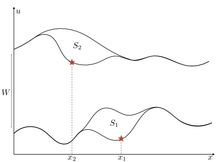
Figure 2: In Section IV.3 we calculate the correlations between the total sizes $S_{1}$ and $S_{2}$ of two avalanches separated by a distance $W$ along $u$, with seeds (i.e. starting points) at $x_{1}$ and $x_{2}$.

IV.3.1 Seed centering and Laplace tranform

The explicit results we have obtained up to know are formally equivalent to the results obtained for shocks in the statics ThieryStaticCorrelations , rederived in the dynamics in a much simpler fashion using our general result (13)-(14)-(15). We now obtained some genuinely new results by looking at the correlations between the total size $S_{1}$ and $S_{2}$ of avalanches occuring at a distance $W$ and having seeds $x_{1}$ and $x_{2}$ (see Fig. 2). By ‘seed’ we mean the first point of the interface that moves when the avalanche starts. This concept is much more natural in the dynamics than in the statics. We now introduce $\rho^{x}(S)$ and $\rho^{x_{1},x_{2}}(S_{1},S_{2})$ the total size density for avalanche that starts at $x$ and total size density for avalanches that starts at $x_{1}$ at $w=0$ and at $x_{2}$ at $w=W$. By translational invariance along the internal direction we have

$$\rho^{x}(S)=\frac{1}{L^{d}}\rho(S)\quad,\quad\rho^{x_{1},x_{2}}_{W}(S_{1},S_{2})\equiv\rho^{x_{2}-x_{1}}_{W}(S_{1},S_{2})\,,$$ (56)

with the normalization

$$\int d^{d}x\rho^{x}_{W}(S_{1},S_{2})=\frac{1}{L^{d}}\rho_{W}(S_{1},S_{2})\,.$$ (57)

Our theory predicts that the Laplace transform of these densities are obtained as in (21)-(22) but with the response fields in front of the exponential not integrated over but restricted at $x_{1}$ or $x_{2}$ (see remark in Sec. LABEL:subsec:analytical:fieldtheory for a justification). More precisely we get

$$\int dS_{1}\rho^{x_{1}}(S_{1})[e^{\lambda_{1}S_{1}}-1]=\int D\tilde{u}_{1}D\dot{u}_{1}\tilde{u}_{1}(x_{1},0)e^{\lambda_{1}\int dx\int_{0}^{+\infty}d\tau_{1}\dot{u}_{1}(x,\tau_{1})-S_{BFM}[\tilde{u}_{1},\dot{u}_{1}]}\,,$$ (58)

and

$$\int dS_{1}dS_{2}\rho_{W}^{x_{1},x_{2}}(S_{1},S_{2})[e^{\lambda_{1}S_{1}}-1][e^{\lambda_{2}S_{2}}-1]$$ (59)

$$=\int D\tilde{u}_{1}D\dot{u}_{1}\int D\tilde{u}_{2}D\dot{u}_{2}\tilde{u}_{1}(x_{1},0)\tilde{u}_{2}(x_{2},0)e^{\sum_{i=1,2}\lambda_{i}\int d^{d}x\int_{0}^{+\infty}d\tau_{i}\dot{u}_{i}(x,\tau_{i})-S[\tilde{u}_{1},\dot{u}_{1},\tilde{u}_{2},\dot{u}_{2}]}\,.$$

IV.3.2 Calculation of the densities

Proceeding as in Sec. IV.1, it is easily seen that the seed centering procedure does not affect the instanton equations satisfied by the response fields and, as mentioned above, the only modification that is necessary is to keep track of the spatial dependence of the solutions of the instanton equation at $x=x_{1}$ and $x=x_{2}$. More precisely, from (58) one easily obtains the trivial result $\rho^{x}(S)=\frac{1}{L^{d}}\rho(S)$ and from (59) one obtains

$$\int dS_{1}dS_{2}\rho_{W}^{x_{1},x_{2}}(S_{1},S_{2})[e^{\lambda_{1}S_{1}}-1][e^{\lambda_{2}S_{2}}-1]=\langle\tilde{u}_{1}(x_{1})\tilde{u}_{2}(x_{2})\rangle_{\xi}\,,$$

with $\tilde{u}_{i}(x_{i})$ still given by the solutions of the instanton equation (29) of Sec. IV.1, a result that should be compared to (33). Using the perturbative solution (32) in adimensioned units we obtain the Laplace transform of the connected density $\rho_{W}^{c,x_{2}-x_{1}}(S_{1},S_{2})=\rho_{W}^{x_{2}-x_{1}}(S_{1},S_{2})-\rho^{x_{1}}(S_{1})\rho^{x_{2}}(S_{2})$ exactly at order $O(\epsilon)$ as

$$\int dS_{1}dS_{2}\rho_{W}^{c,x_{2}-x_{1}}(S_{1},S_{2})[e^{\lambda_{1}S_{1}}-1][e^{\lambda_{2}S_{2}}-1] =-\hat{\Delta}^{\prime\prime}(W)\int\frac{d^{d}q}{(2\pi)^{d}}e^{iq(x_{1}-x_{2})}\frac{Z(\lambda_{1})}{1-2Z(\lambda_{1})+q^{2}}\frac{Z(\lambda_{2})}{1-2Z(\lambda_{2})+q^{2}}\,.$$

This can be explicitly computed and we obtain the following exact result ($O(\epsilon)$) for this Laplace transform

$$\int dS_{1}dS_{2}\rho_{W}^{c,x_{2}-x_{1}}(S_{1},S_{2})[e^{\lambda_{1}S_{1}}-1][e^{\lambda_{2}S_{2}}-1]=-\hat{\Delta}^{\prime\prime}(W)Z(\lambda_{1})Z(\lambda_{2}){\cal{I}}(1-2Z(\lambda_{1}),1-2Z(\lambda_{2}),|x_{1}-x_{2}|)$$

$${\cal{I}}(a,b,x)=\int\frac{d^{d}q}{(2\pi)^{d}}\frac{e^{iqx}}{(a+q^{2})(b+q^{2})}=\frac{1}{b-a}\left(\tilde{{\cal{I}}}(a,x)-\tilde{{\cal{I}}}(b,x)\right)$$

$$\tilde{{\cal{I}}}(a,x)=\frac{1}{(2\pi)^{d/2}}a^{\frac{d-2}{4}}x^{\frac{2-d}{2}}K_{\frac{d-2}{2}}(\sqrt{a}x)\,.$$ (60)

This is an exact expression but not easy to inverse Laplace transform to obtain the density. For that purpose it is more convenient to work in Fourier space, defining $\rho_{W}^{q}(S_{1},S_{2})=\int d^{d}xe^{iqx}\rho_{W}^{x}(S_{1},S_{2})$. We obtain for the connected part

$$\rho_{W}^{c,q}(S_{1},S_{2})=-\hat{\Delta}^{\prime\prime}(W)\psi_{q}(S_{1})\psi_{q}(S_{2})\,,$$ (61)

where we have introduced the function $\psi_{q}(S)$ defined as

$$\psi_{q}(S)=\hat{\rho}(S)(1+q^{2})\frac{S}{2}\left(1-\frac{\sqrt{\pi S}}{2}q^{2}e^{\frac{q^{4}S}{4}}{\rm Erfc}(\frac{q^{2}\sqrt{S}}{2})\right)\,,$$ (62)

with $\hat{\rho}(S)$ still given by (26), and whose Laplace transform is

$$\int dS(e^{\lambda S}-1)\psi_{q}(S)=\frac{Z(\lambda)}{1-2Z(\lambda)+q^{2}}\,.$$ (63)

We give here a few of the lowest order moments of the function $\psi_{q}(S)$:

$$\int\psi_{q}(S)dS=\frac{1}{2}\quad,\quad\int\psi_{q}(S)SdS=\frac{1}{1+q^{2}}\quad,\quad\int\psi_{q}(S)S^{2}dS=\frac{2(3+q^{2})}{(1+q^{2})^{2}}\,.$$ (64)

The zeroth order moment allows for example to calculate from (61) the connected total density of avalanches with seeds $x_{1}$ and $x_{2}$

$$\rho_{2}^{c}(W,x_{2}-x_{1}):=\int dS_{1}dS_{2}\rho_{W}^{c,x_{2}-x_{1}}(S_{1},S_{2})=-\frac{\hat{\Delta}^{\prime\prime}(W)}{4}\delta^{d}(x_{2}-x_{1})$$ (65)

The form of the result shows that the drop in density of avalanche at $w=W$ caused by the occurence of an avalanche at $w=0$ with seed $x_{1}$ is only felt at microscopic distances. This is not so surprising since the vast majority of avalanches are of microscopic sizes (the density $\rho^{x}(S)$ is not normalizable at small $S$). By contrast, the first joint moment (obtained from the second identity in (64)) is dominated by large avalanches and reads

$$\langle S_{1}S_{2}\rangle_{\rho_{W}^{c,x}}:=\int dS_{1}dS_{2}S_{1}S_{2}\rho_{W}^{c,x}(S_{1},S_{2})=-\hat{\Delta}^{\prime\prime}(W)2^{-1-d/2}\pi^{-d/2}x^{2-\frac{d}{2}}K_{\frac{d-4}{2}}(x)\,.$$ (66)

Integrating this result over $x$ leads to the exact relation $L^{-2d}\langle S_{1}S_{2}\rangle_{W}^{c}=-\frac{\hat{\Delta}^{\prime\prime}(W)}{L^{d}}$. This suggests that the above result may be quite accurate since it integrates to an exact result. Suprisingly, the full $x$ dependence of this first joint moment is identical to the one of the correlation of the local sizes when the driving is uniform, see Eq. 112 in ThieryStaticCorrelations . This surprising result does not hold for higher order moments as can easily be seen by comparing the formulas.

IV.3.3 Universality and the massless limit

We now address in more depth the issue of universality and of the massless limit. In Section IV.1.3 we obtained a universal scaling form (38) for $\rho^{c}_{W}(S_{1},S_{2})$. This form however involves two features which makes it not fully universal. (i) First it depends explicitly on $m$ and $S_{m}$, i.e. it is universal (i.e. independent of small scale details) within the model of the driving parabolic well, which provides a large scale cutoff. One can ask if it is possible to obtain results for avalanche correlations which would be independent of the details of large scale cutoff (which we call full universality). (ii) The second feature is that $\rho^{c}_{W}(S_{1},S_{2})$ is proportional to $(mL)^{d}$, i.e. the number of independent regions along the interface. This makes sense since avalanches are expected to be correlated only if they are separated within a distance $x\sim 1/m$ along the interface.

In the above calculation of $\rho^{c,x}_{W}(S_{1},S_{2})$ the factor $(mL)^{d}$ is absent, since the separation of the seeds, $x$, is fixed. In Fourier space we now expect, restoring units

$$\rho_{W}^{c,q}(S_{1},S_{2})=\frac{1}{m^{d}S_{m}^{4}}{\cal F}_{d}(\frac{q}{m},\frac{W}{W_{m}},\frac{S_{1}}{S_{m}},\frac{S_{2}}{S_{m}})$$ (67)

where ${\cal F}_{d}$ is a universal function. From our result (61) we see that, restoring units, with $w=W/W_{m}$ one has the expansion around the upper critical dimension

$${\cal F}_{d}(q,w,s_{1},s_{2})=-m^{d-4}\Delta^{\prime\prime}(W)\psi_{q}(s_{1})\psi_{q}(s_{2})+O(\epsilon^{2})=-A_{d}\tilde{\Delta}^{*\prime\prime}(w)\psi_{q}(s_{1})\psi_{q}(s_{2})+O(\epsilon^{2})$$ (68)

where all factors are universal using the fixed point (17) (apart for a single non-universal scale, see discussion below (39)).

Let us now discuss the behavior of (67) in the region $q\gg m$, $S_{i}\ll S_{m}$, $W\ll W_{m}$ where we hope to find a fully universal behavior. It is equivalent to take $m\to 0$ and consider the massless limit. It turns out that consideration of this limit, upon some hypothesis, leads a host of information, i.e. determination of some critical exponents.

Let us first recall the analysis of the massless limit for the single avalanche size density, $\rho(S)$, and its connection to the Narayan-Fisher conjecture NarayanDSFisher1992b ; NarayanDSFisher1993a .

The massless limit of the starting equation of motion for the interface, Eq. (1), is obtained by defining $f(x,t)=m^{2}w(x,t)$, the applied force. One can then take $m\to 0$ at fixed $f(x,t)$ and the equation remains well defined. Then one must define densities per unit force, denoted everywhere with a subscript $f$, rather than per unit $w$ as we did until now. They simply differ by the factor $m^{2}$, e.g.

$$\rho^{f}(S)=m^{-2}\rho(S)$$ (69)

It is easy to see on the result for the BFM (26) that the massless limit of $\rho^{f}(S)$ is well defined (i.e. all factors of $m$ cancel) leading to

$$\rho^{f}(S)=\lim_{m\to 0}m^{-2}\rho(S)=\frac{L^{d}}{\sigma^{1/2}}\frac{1}{2\sqrt{\pi}S^{3/2}}$$ (70)

which is the fully universal part of the density corresponding to small avalanches $S\ll S_{m}$. It turns out that this extends beyond mean field. Indeed, for any $d$ one has, via simple dimensional analysis

$$\rho(S)=\frac{L^{d}}{S_{m}^{2}}r(S/S_{m})\quad,\quad r(s)\sim_{s\to 0}s^{-\tau}$$ (71)

where $\tau$ is the avalanche size exponent. For $\rho^{f}(S)=\lim_{m\to 0}m^{-2}\rho(S)$ to be finite, we see that we need $m^{-2}S_{m}^{\tau-2}$ to be finite in the limit $m\to 0$, and using $S_{m}\sim m^{-(d+\zeta)}$ this is equivalent to

$$\tau=\tau_{\rm NF}=2-\frac{2}{d+\zeta}$$ (72)

This relation was tested to one loop in LeDoussalWiese2012a , and is rather natural since we do expect that a universal massless limit exists (a massless field theory). We will thus generally assume that densities per unit force do exist in the limit $m\to 0$. This led in DobrinevskiLeDoussalWiese2014a to predictions for a number of other avalanche exponents, and we call it the generalized NF conjecture.

Consider now the massless limit of the joint size density to which we apply similar arguments. We note from (62) that

$$\lim_{m\to 0}m^{4}\psi_{q/m}(\frac{S}{S_{m}})=\frac{\sigma}{S}\psi(q(S/\sigma)^{1/4})$$ (73)

$$\psi(q)=\frac{q^{2}}{4\sqrt{\pi}}-\frac{1}{8}e^{\frac{q^{4}}{4}}q^{4}\text{erfc}\left(\frac{q^{2}}{2}\right)=\frac{q^{2}}{4\sqrt{\pi}}+O(q^{4})=\frac{1}{2\sqrt{\pi}q^{2}}+O\left(\frac{1}{q^{4}}\right)$$ (74)

where $\psi(q)$ is the massless scaling form of $\psi_{q}(S)$. Thus our result to $O(\epsilon)$ for the joint density per unit force has a well defined $m\to 0$ limit

$$\rho_{W}^{c,q,f}(S_{1},S_{2})=\lim_{m\to 0}m^{-4}\rho_{W}^{c,q}(S_{1},S_{2})=-\frac{\Delta^{\prime\prime}(W)}{\sigma^{2}}\frac{1}{S_{1}S_{2}}\psi(q(S_{1}/\sigma)^{1/4})\psi(q(S_{2}/\sigma)^{1/4})+O(\epsilon^{2})$$ (75)

Note that as $m\to 0$, $\Delta^{\prime\prime}(W)=A_{d}m^{\epsilon}\tilde{\Delta}^{*\prime\prime}(Wm^{\zeta})\simeq A_{d}\tilde{\Delta}^{*\prime\prime}(0^{+})+O(\epsilon^{2})$ if $W$ is kept fixed as $m\to 0$. Hence the dependence in $W$ disappears in that limit since there can be avalanches of arbitrary sizes, all avalanches can be considered as successive (i.e. $W=0^{+}$).

More generally, we surmise that this massless limit exist in any dimension. Scaling arguments and dimensional analysis then lead to the scaling form

$$\rho_{W}^{c,q,f}(S_{1},S_{2})=\frac{\ell_{\sigma}^{d+4}}{(S_{1}S_{2})^{\tau_{c}^{1}}}~{}f_{d}(\ell_{\sigma}\,qS_{1}^{1/(d+\zeta)},\ell_{\sigma}\,qS_{2}^{1/(d+\zeta)})\quad,\quad\tau_{c}^{1}=\frac{1}{2}(2-\frac{4-d-2\zeta}{d+\zeta})$$ (76)

where $\tau_{c}^{1}$ is a correlation exponent, $f_{d}$ is a fully universal function and the scale $\ell_{\sigma}$ is non fully universal . For the parabolic well model it equals $\ell_{\sigma}=\lim_{m\to 0}m^{-1}S_{m}^{-1/(d+\zeta)}$ (hence can be measured independently using (37)), as easily seen by studying the possible $m\to 0$ limit of the scaling function ${\cal F}_{d}$ in (67).

We see that for $d=4-\epsilon$ and $\zeta=O(\epsilon)$ the form (76) reproduces (75) with $\ell_{\sigma}=\sigma^{-1/4}$ and

$$f_{d}(q_{1},q_{2})=-A_{d}\tilde{\Delta}^{*\prime\prime}(0^{+})\psi(q_{1})\psi(q_{2})+O(\epsilon^{2})=-\frac{16\pi^{2}\epsilon}{9}\psi(q_{1})\psi(q_{2})+O(\epsilon^{2})$$ (77)

where $\psi(q)$ is given in (74).

Let us now study the $q=0$ limit, i.e. the uniform driving studied in Section IV.1.3. For a fixed $m>0$ one has

$$\rho_{W}^{c}(S_{1},S_{2})=L^{d}\rho_{W}^{c,q=0}(S_{1},S_{2})=-\frac{L^{d}}{m^{d}S_{m}^{4}}m^{d-4}\Delta^{\prime\prime}(W)\frac{S_{1}S_{2}}{4S_{m}^{2}}\hat{\rho}(S_{1}/S_{m})\hat{\rho}(S_{2}/S_{m})$$ (78)

using (67), (68), and, from (62), that $\psi_{q=0}(s)=\hat{\rho}(s)\frac{s}{2}$. It coincides with (36) upon using (26). Its $m\to 0$ limit reads

$$\rho_{W}^{c,f}(S_{1},S_{2})=m^{-4}\rho_{W}^{c}(S_{1},S_{2})=-(mL)^{d}\frac{A_{4}\tilde{\Delta}^{*\prime\prime}(0^{+})}{\sigma^{3}}\frac{1}{16\pi S_{1}^{1/2}S_{2}^{1/2}}+O(\epsilon^{2})\,,$$ (79)

Note that this result cannot be obtained from taking the $q\to 0$ limit of (75) since $\psi(q)\sim q^{2}$ as $q\to 0$. Hence there is a non-commutation of limits $m\to 0$ and $q\to 0$.

It is reasonable to surmise that in any dimension, as $m\to 0$

$$\rho_{W}^{c,f}(S_{1},S_{2})\sim(mL)^{d}\frac{1}{S_{1}^{\tau_{c}}S_{2}^{\tau_{c}}}$$ (80)

with $\tau_{c}=1/2$ in mean-field, i.e. for $d=d_{c}=4$ here, the factor $(mL)^{d}$ being the number of independent regions. One can obtain this factor by considering the $q\to 0$ limit of the massless result on one hand, and the $q=0$ massive result at small $m$ on the other, and requiring matching upon setting $q=m$. This determines the $q\to 0$ behavior of the scaling function $f_{d}$ as

$$f_{d}(qS_{1}^{1/(d+\zeta)},qS_{2}^{1/(d+\zeta)})\simeq_{q\to 0}q^{d}(S_{1}S_{2})^{\frac{1}{2}\frac{d}{d+\zeta}}$$ (81)

So that, substituting $q=m$ in (76) we indeed obtain

$$\rho_{W}^{c,f}(S_{1},S_{2})=L^{d}\rho_{W}^{c,q=m,f}(S_{1},S_{2})\sim(Lm)^{d}\frac{1}{S_{1}^{\tau_{c}}S_{2}^{\tau_{c}}}\quad,\quad\tau_{c}=2-\frac{2+d}{d+\zeta}$$ (82)

where the exponent $\tau_{c}$ is thus fully determined, via this generalized NF argument (recovering $\tau_{c}=1/2$ in mean-field for $d=4$, $\zeta=0$).

V Numerics

In this section we compare some of our results with the simulation of a $d=1$ elastic interface with short-ranged elasticity in a short-ranged correlated disordered landscape.

V.1 Protocol

To perform numerical simuations we choose a Gaussian disorder $F(u,x)$ with a correlator $\overline{F(u,x)F(u^{\prime},x^{\prime})}=\delta(x-x^{\prime})\Delta_{0}(u-u^{\prime})$ with $\Delta_{0}(u)=\sigma\delta ue^{-|u|/\delta u}$ with $\delta u$ the microscopic correlation length of the disorder. As explained in ThieryShape , this can be realized by taking $F(u,x)$ as a collection (indexed by $x$) of independent Ornstein-Uhlenbeck processes (in the direction $u$). More precisely the model we study can be defined as, for any driving protocol $w(x,t)$

$$\eta\partial_{t}u(x,t)=\nabla^{2}_{x}u(x,t)-m^{2}(u(x,t)-w(x,t))+F(u(x,t),x)$$

$$\partial_{u}F(u,x)=\sqrt{2\sigma}\xi(u,x)-\frac{1}{\delta u}F(u,x)\,.$$ (83)

with $\xi(u,x)$ a unit centered two dimensional Gaussian white noise $\overline{\xi(u,x)\xi(u^{\prime},x^{\prime})}=\delta(u-u^{\prime})\delta(x-x^{\prime})$. The advantage of this setup is that one can directly obtain an autonomous equation for the velocity field $\dot{u}(x,t)$: the above model is equivalent to

$$\eta\dot{u}(x,t)=\nabla^{2}\dot{u}(x,t)+m^{2}(\dot{w}(t)-\dot{u}(x,t))+\partial_{t}{\sf F}(x,t)\ ,$$

$$\partial_{t}{\sf F}(x,t)=\sqrt{2\sigma\dot{u}(x,t)}\chi(x,t)-\frac{\dot{u}(x,t)}{\delta u}{\sf F}(x,t)\ ,$$ (84)

with $\chi(x,t)$ a centered Gaussian white noise $\overline{\chi(x,t)\chi(x^{\prime},t^{\prime})}=\delta^{d}(x-x^{\prime})\delta(t-t^{\prime})$ and we have the equality in law ${\sf F}(x,t)\sim F(x,u(x,t))$.

We take as initial conditions $\dot{u}(x,t=0)={\sf F}(x,t=0)=0$ and then apply a sequence of kicks of size $\delta w=1$, which amounts at setting $\dot{u}(x,t)=\frac{m^{2}}{\eta}\delta w$ at the beginning of each kick and wait for the interface to stop before applying the next kick. The motion of the interface between each kick is measured by integrating the velocity field in between two kicks and this defines for each kick an avalanche $S_{x}$. The avalanche at the $n$-th kick is said to have been triggered at $w=n\delta w$. We wait for the sytem to reach a stationary state before measuring anything. Averages are obtained using $50$ independent ‘experience’, each experience consisting in $2\times 10^{6}$ kicks, and we have thus simulated $10^{8}$ avalanches. Correlations between avalanches are measured for avalanches inside a window of $1000$ successive kicks.

In the results reported here we have taken an interface of lateral extension $L=1024$ with periodic boundary conditions, discretized with $1024$ points. The parameters are chosen as $m=20/L\simeq 0.02$. The kicks are of size $\delta w=1$ and the microscopic disorder correlation length is taken as $\delta u=5\delta w=5$. The discretization in time is handled using an algorithm similar as the one introduced in Dornic and we take a time step $\delta t=0.025$.

V.2 Results

V.2.1 Renormalized disorder correlator

Central to our results is the measurement of the renormalized disorder second cumulant $\Delta(w-w^{\prime})=L^{d}m^{4}\overline{(u(w)-w)(u(w^{\prime})-w^{\prime})}^{c}$ where $u(w)$ is the position of the interface in the end of the $w/\delta w$-th kick. The plot of $\Delta(w)$ is presented in Fig. 3. To obtain a good measurement of the derivative $\Delta^{\prime}(w)$ and $\Delta^{\prime\prime}(w)$ we fitted $\Delta(w)$ with a polynomial of order seven and differentiated directly the fitted polynomial. A plot of $\Delta^{\prime}(w)$ and $\Delta^{\prime\prime}(w)$ is also given in Fig. 4.

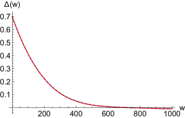
Figure 3: The renormalized disorder second cumulant measured in the simulations (blue dots) and its polynomial fit (red line).

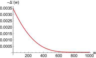
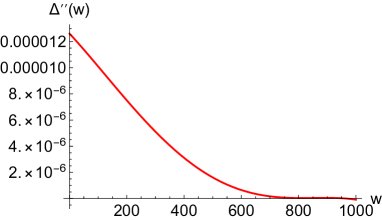
Figure 4: First (left figure) and second (right figure) derivative of the renormalized disorder second cumulant as obtained using the polynomial fit of the measured renormalized disorder second cumulant.

V.2.2 Total avalanche sizes correlations

We show in Fig. 5 the comparison between the measurements of $\langle S_{1}S_{2}\rangle_{W}^{c}$ and $\frac{1}{2}\left(\langle S_{1}S_{2}^{2}\rangle_{W}^{c}+\langle S_{1}^{2}S_{2}\rangle_{W}^{c}\right)$ and our predictions (34)-(35). The analytical result for $\langle S_{1}S_{2}\rangle_{W}^{c}$ is exact and the agreement is as expected perfect. The analytical result for $\frac{1}{2}\left(\langle S_{1}S_{2}^{2}\rangle_{W}^{c}+\langle S_{1}^{2}S_{2}\rangle_{W}^{c}\right)$ is only a $O(\epsilon)$ approximation and appears to overestimate the correlations.

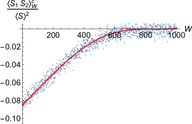
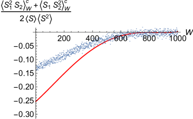
Figure 5: Left: Comparison between the measurement of $\langle S_{1}S_{2}\rangle_{W}^{c}$ (blue dots) and our prediction (34) (exact result). Right: Comparison between the measurement of $\frac{1}{2}\left(\langle S_{1}S_{2}^{2}\rangle_{W}^{c}+\langle S_{1}^{2}S_{2}\rangle_{W}^{c}\right)$ (blue dots) and our prediction (35) (order $O(\epsilon)$ result). The blue dots corresponds to direct measurements of the correlations between avalanches, each dot corresponding to an average over avalanches for a given $W$. The dispersion of the cloud of dots gives an estimate of the accuracy of the measurement.

V.2.3 Local avalanche sizes correlations

We show in Fig. 6 the comparison between the measurements of $\langle S_{10}S_{2x}\rangle_{W}^{c}$ and our prediction (55). Despite the fact that (55) is only valid up to order $O(\epsilon)$ (with here $\epsilon=3$), it is clear that it is a very good approximation. Also it seems that our result tends to slightly underestimate the correlations between avalanches at short distance and overestimate the correlations at large distance.

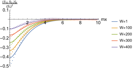
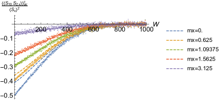
Figure 6: Comparison between the measurement of $\langle S_{10}S_{2x}\rangle_{W}^{c}$ (dots) and our prediction (55) (plain and dashed lines, order $O(\epsilon)$ approximation) as a function of $mx$ for a few values of $W$ (left) or as a function of $W$ for a few values of $mx$ (right).

VI Analytical results: Dynamical correlations

VI.1 Correlations of the total velocities in an avalanche, and of the avalanche durations

In this Section we study the correlation of the global velocities (center of mass velocities) in the two avalanches. As a by product we also obtain the correlation between the avalanche durations. Let us define the total (areal) velocities in the two avalanches, which we denote $\dot{u}_{1}\equiv\dot{u}_{1}(t_{1})=\int d^{d}x\dot{u}_{1}(x,t_{1})$ and $\dot{u}_{1}\equiv\dot{u}_{2}(t_{2})=\int d^{d}x\dot{u}_{1}(x,t_{2})$. The time is counted from the kick in each avalanche, i.e. each avalanche starts at $t_{i}=0$.

Similar methods as in Section IV.2 give, for the joint density $\rho^{x_{1},x_{2}}_{W}(\dot{u}_{1},\dot{u}_{2})$ at fixed positions of the seeds $x_{1},x_{2}$

$$\int d\dot{u}_{1}d\dot{u}_{2}\rho^{x_{1},x_{2}}_{W}(\dot{u}_{1},\dot{u}_{2})[e^{\lambda_{1}\dot{u}_{1}}-1][e^{\lambda_{2}\dot{u}_{2}}-1]=\langle\tilde{u}_{1}(x_{1},0)\tilde{u}_{2}(x_{2},0)\rangle_{\xi}$$ (85)

where $\tilde{u}_{i}(x,t)$ are the solutions of the time-dependent space inhomogeneous instanton equation

$$(\partial_{t}+\nabla_{x}^{2}-1)\tilde{u}_{i}(x,t)+\tilde{u}_{i}(x,t)^{2}=-\xi_{i}(x)\tilde{u}_{i}(x,t)-\lambda_{i}\delta(t-t_{i})$$ (86)

with $\tilde{u}_{i}(x,t>t_{i})=0$, which are needed only to first order in each $\xi_{i}$. As in Section IV.2 we introduce

$$\tilde{u}_{i}(x,t)=\tilde{u}^{0}_{i}(t)+\tilde{u}^{1}_{i}(x,t)$$ (87)

where $\tilde{u}^{0}_{i}(t)$ is the solution for $\xi_{i}(x)=0$, which satisfies

$$(\partial_{t}-1)\tilde{u}^{0}_{i}(t)+\tilde{u}^{0}_{i}(t)^{2}=-\lambda_{i}\delta(t-t_{i})$$ (88)

with $\tilde{u}^{0}_{i}(t>t_{i})=0$. The solution is well known to be LeDoussalWiese2011a

$$\tilde{u}_{i}^{0}(t)=\frac{\lambda_{i}}{\lambda_{i}+(1-\lambda_{i})e^{t_{i}-t}}\theta(t<t_{i})$$ (89)

Let us recall that from this solution one obtains the single avalanche (time-dependent) density in the BFM, denoted $\rho(\dot{u})\equiv\rho_{t}(\dot{u})$, of the total velocity $\dot{u}(t)=\int d^{d}x\dot{u}(x,t)$, by Laplace inversion of

$$\int_{0}^{+\infty}d\dot{u}\rho_{t}(\dot{u})(e^{\lambda\dot{u}}-1)=L^{d}\tilde{u}^{0}(0)=L^{d}\frac{\lambda}{\lambda+(1-\lambda)e^{t}}\quad\Rightarrow\quad\rho_{t}(\dot{u})=L^{d}\frac{e^{t-\frac{e^{t}\dot{u}}{e^{t}-1}}}{\left(e^{t}-1\right)^{2}}\quad,\quad\dot{u}>0$$ (90)

By integration over time one recovers the well known result for the mean density of total velocity $\rho_{v=0^{+}}(\dot{u})$ for a uniform driving in the limit $v=0^{+}$, $\rho_{v=0^{+}}(\dot{u})=\int_{0}^{+\infty}dt\rho_{t}(\dot{u})=\frac{L^{d}}{\dot{u}}e^{-\dot{u}}$ (see LeDoussalWiese2011a ; LeDoussalWiese2012a ; ABBMNonstat2012 ). The same calculation also gives the density of the avalanche duration $T$ in the BFM

$$\rho(T)=-\partial_{t}\int_{0}^{+\infty}d\dot{u}\rho_{t}(\dot{u})|_{t=T}=\frac{L^{d}}{4\sinh^{2}(T/2)}$$ (91)

which reads, in dimensionfull units, $\rho(T)=\frac{L^{d}}{S_{m}\tau_{m}4\sinh^{2}(T/2\tau_{m})}$.

To obtain the connected joint density, we need to calculate $\tilde{u}^{1}_{i}(x,t)$ to first order in $\xi_{i}$. For that purpose we introduce the dressed response kernel

$$(\partial_{t}+\nabla_{x}^{2}-1+2\tilde{u}_{i}^{0}(t))G_{i}(x,t;y,t^{\prime})=-\delta^{d}(x-y)\delta(t-t^{\prime})\,.$$ (92)

with $G_{i}(x,t;y,t^{\prime})=0$ for $t>t^{\prime}$ (i.e. time is in effect reversed as compared to a standard response function). It reads in Fourier, for $t,t^{\prime}<t_{i}$

$$G_{i}(q,t,t^{\prime}) = e^{-(q^{2}+1)(t^{\prime}-t)+2\int_{t}^{t^{\prime}}\tilde{u}_{i}^{0}(s)ds}\theta(t^{\prime}-t)$$

$$= e^{-(q^{2}+1)(t^{\prime}-t)}\frac{(1-\lambda_{i}+\lambda_{i}e^{t^{\prime}-t_{i}})^{2}}{(1-\lambda_{i}+\lambda_{i}e^{t-t_{i}})^{2}}\theta(t^{\prime}-t)$$

We obtain

$$\tilde{u}^{1}_{i}(x,t)=\int d^{d}y\,G_{i}(x,t;y,t^{\prime})\xi_{i}(y)\tilde{u}_{i}^{0}(t^{\prime})+O(\xi^{2})$$ (94)

which leads to the Laplace transform of the connected density as

$$\int d\dot{u}_{1}d\dot{u}_{2}\rho^{c,x_{1},x_{2}}_{W}(\dot{u}_{1},\dot{u}_{2})[e^{\lambda_{1}\dot{u}_{1}}-1][e^{\lambda_{2}\dot{u}_{2}}-1]$$ (95)

$$=-\hat{\Delta}^{\prime\prime}(W)\int d^{d}y\int_{0}^{t_{1}}dt^{\prime}\int_{0}^{t_{2}}dt^{\prime\prime}G_{1}(x_{1},0;y,t^{\prime})G_{2}(x_{2},0;y,t^{\prime\prime})\tilde{u}^{0}_{1}(t^{\prime})\tilde{u}^{0}_{2}(t^{\prime\prime})\,.$$

It is more convenient to work in Fourier space and define

$$\rho^{c,x_{1},x_{2}}_{W}(\dot{u}_{1},\dot{u}_{2})=\int\frac{d^{d}q}{(2\pi)^{d}}e^{-iq(x_{1}-x_{2})}\rho^{c,q}_{W}(\dot{u}_{1},\dot{u}_{2})$$ (96)

We finally obtain the Laplace transform of the connected part of the joint density of total velocities in the two avalanches, for a fixed driving wavevector $q$ as

$$\int d\dot{u}_{1}d\dot{u}_{2}\rho^{c,q}_{W}(\dot{u}_{1},\dot{u}_{2})[e^{\lambda_{1}\dot{u}_{1}}-1][e^{\lambda_{2}\dot{u}_{2}}-1]=-\hat{\Delta}^{\prime\prime}(W)F_{\lambda_{1}}(q,t_{1})F_{\lambda_{2}}(q,t_{2})$$ (97)

where we have defined

$$F_{\lambda}(q,t)=\lambda\frac{\left(1-q^{2}-\lambda\right)e^{-(1+q^{2})t}+(1-\lambda)\left(q^{2}-1\right)e^{-t}+\lambda q^{2}e^{-2t}}{q^{2}\left(q^{2}-1\right)\left(1-\lambda+\lambda e^{-t}\right)^{2}}$$ (98)

We now analyze this formula in various cases: (i) homogeneous driving (ii) fixed distance between the seeds (iii) massless limit (leading to conjectures for the correlation exponents in any dimension).

VI.1.1 Homogeneous driving

Velocities. For the homogeneous driving $\delta w(x)=\delta w$, the Laplace transform of the connected joint density simplifies into

$$\int d\dot{u}_{1}d\dot{u}_{2}\rho^{c}_{W}(\dot{u}_{1},\dot{u}_{2})[e^{\lambda_{1}\dot{u}_{1}}-1][e^{\lambda_{2}\dot{u}_{2}}-1]=-L^{d}\hat{\Delta}^{\prime\prime}(W)F_{\lambda_{1}}(t_{1})F_{\lambda_{2}}(t_{2})$$ (99)

where we denote

$$F_{\lambda}(t)=F_{\lambda}(q=0,t)=-\frac{\lambda e^{-t}\left(\lambda\left(t-1+e^{-t}\right)-t\right)}{\left(1-\lambda+\lambda e^{-t}\right)^{2}}$$ (100)

It is possible to perform the inverse Laplace transform explicitly and obtain

$$\rho^{c}_{W}(\dot{u}_{1},\dot{u}_{2})=-L^{d}\hat{\Delta}^{\prime\prime}(W)~{}r_{t_{1}}(\dot{u}_{1})\,r_{t_{2}}(\dot{u}_{2})$$ (101)

$$r_{t}(\dot{u})=\frac{e^{t-\frac{e^{t}u}{e^{t}-1}}\left(e^{t}\left(-(t+1)\dot{u}+e^{t}(t+\dot{u}-2)+4\right)-t-2\right)}{\left(e^{t}-1\right)^{4}}=\frac{d}{dt}\frac{\left(-t+e^{t}-1\right)e^{t-\frac{e^{t}\dot{u}}{e^{t}-1}}}{\left(e^{t}-1\right)^{2}}$$ (102)

Restoring the units it reads

$$\rho^{c}_{W}(\dot{u}_{1},\dot{u}_{2})=-\frac{L^{d}}{m^{4}v_{m}^{2}S_{m}^{2}}\Delta^{\prime\prime}(W)\,r_{t_{1}/\tau_{m}}(\frac{\dot{u}_{1}}{v_{m}})r_{t_{2}/\tau_{m}}(\frac{\dot{u}_{2}}{v_{m}})$$ (103)

where $v_{m}=S_{m}/\tau_{m}$. One can check that $\int_{0}^{+\infty}dt_{1}\int_{0}^{+\infty}dt_{2}\langle\dot{u}_{1}\dot{u}_{2}\rangle_{W}^{c}$ calculated with this formula coincides with the result for $\langle S_{1}S_{2}\rangle_{W}^{c}$ obtained above in (34) (which, we recall was an exact result, i.e. valid beyond the $\epsilon$ expansion).

We can calculate the joint density of the mean total velocity, averaged over all the avalanche. In dimensionless units, using that $\int_{0}^{+\infty}dt\,r_{t}(\dot{u})=e^{-\dot{u}}$, it reads simply

$$\int_{0}^{+\infty}dt_{1}\int_{0}^{+\infty}dt_{2}\rho^{c}_{W}(\dot{u}_{1},\dot{u}_{2})=-L^{d}\hat{\Delta}^{\prime\prime}(W)e^{-\dot{u}_{1}-\dot{u}_{2}}$$ (104)

Note that it is regular at small $\dot{u}$, unlike the single avalanche density (see above) $\rho(\dot{u})=\frac{1}{\dot{u}}e^{-\dot{u}}$.

Let us obtain some cumulants. One has (in dimensionfull units)

$$\frac{\langle\dot{u}_{1}\dot{u}_{2}\rangle^{c}_{W}}{\langle\dot{u}_{1}\rangle\langle\dot{u}_{2}\rangle}=-\frac{\Delta^{\prime\prime}(W)}{m^{4}L^{d}}\frac{t_{1}t_{2}}{\tau_{m}^{2}}$$ (105)

and (in dimensionless units)

$$\frac{\langle\dot{u}_{1}\dot{u}_{2}^{3}\rangle^{c}_{W}}{\langle\dot{u}_{1}^{2}\dot{u}_{2}^{2}\rangle^{c}_{W}}=\frac{3e^{t_{1}-t_{2}}\left(e^{t_{2}}-1\right)\left(-3t_{2}+e^{t_{2}}\left(t_{2}+2\right)-2\right)}{2\left(-2t_{1}+e^{t_{1}}\left(t_{1}+1\right)-1\right)\left(-2t_{2}+e^{t_{2}}\left(t_{2}+1\right)-1\right)}$$ (106)

Durations. Finally we can obtain the correlation between the durations $T_{1}$ and $T_{2}$ of the two avalanches. Integrating over $\dot{u}$

$$\int_{0}^{+\infty}d\dot{u}\,r_{t}(\dot{u})=\frac{e^{t}(t-1)+1}{\left(e^{t}-1\right)^{2}}$$ (107)

hence we obtain

$$\rho^{c}_{W}(T_{1},T_{2})=-L^{d}\hat{\Delta}^{\prime\prime}(W)d(T_{1})d(T_{2})$$ (108)

$$d(T)=-\partial_{T}\int_{0}^{+\infty}d\dot{u}\,r_{T}(\dot{u})=\frac{e^{T}\left(e^{T}(T-2)+T+2\right)}{\left(e^{T}-1\right)^{3}}\simeq_{T\ll 1}\frac{1}{6}-\frac{T^{2}}{60}+O\left(T^{3}\right)$$ (109)

$$~{}~{}~{}~{}~{}~{}~{}~{}~{}~{}~{}~{}~{}~{}~{}~{}~{}~{}~{}~{}~{}~{}~{}~{}~{}~{}~{}~{}~{}~{}~{}~{}~{}~{}~{}~{}~{}~{}~{}~{}~{}~{}~{}~{}~{}~{}~{}~{}~{}~{}~{}~{}~{}~{}~{}~{}~{}~{}~{}~{}~{}~{}~{}~{}~{}~{}~{}~{}~{}~{}\simeq_{T\gg 1}\simeq Te^{-T}$$ (110)

where $d(T)$ is a decreasing function of $T$. Note that the dimensionful version is

$$\rho^{c}_{W}(T_{1},T_{2})=-\frac{L^{d}}{m^{4}S_{m}^{2}\tau_{m}^{2}}\Delta^{\prime\prime}(W)d(T_{1}/\tau_{m})d(T_{2}/\tau_{m})$$ (111)

VI.1.2 Fixed distance between the seeds.

Velocities. We now calculate the connected joint density $\rho^{c,x}_{W}(\dot{u}_{1},\dot{u}_{2})$, for the total velocities (at times $t_{1}$ and $t_{2}$ respectively) of two avalanches starting a distance $x$ apart (i.e. in $x_{1}$ and $x_{2}$ with $x_{2}-x_{1}=x$). The definitions are similar to those in Section IV.3. One finds

$$\rho^{c,x}_{W}(\dot{u}_{1},\dot{u}_{2})=\int\frac{d^{d}q}{(2\pi)^{d}}\,e^{iqx}\,\rho^{c,q}_{W}(\dot{u}_{1},\dot{u}_{2})$$ (112)

$$\rho^{c,q}_{W}(\dot{u}_{1},\dot{u}_{2})=-\hat{\Delta}^{\prime\prime}(W)~{}r_{q,t_{1}}(\dot{u}_{1})r_{q,t_{2}}(\dot{u}_{2})$$ (113)

where

$$r_{q,t}(\dot{u})=\frac{e^{-q^{2}t-\frac{e^{t}\dot{u}}{e^{t}-1}+t}}{q^{2}\left(q^{2}-1\right)\left(e^{t}-1\right)^{4}}(A(q,t)+\dot{u}B(q,t))$$ (114)

$$B(q,t)=e^{t}(-q^{2}e^{t}+e^{q^{2}t}+q^{2}-1)$$ (115)

$$A(q,t)=-2q^{2}e^{t}-2q^{2}e^{q^{2}t+t}+(q^{2}-1)(1+e^{(q^{2}+2)t})+(q^{2}+1)(e^{2t}+e^{q^{2}t})$$ (116)

Restoring the units it reads

$$\rho^{c,q}_{W}(\dot{u}_{1},\dot{u}_{2})=-\frac{1}{m^{4}v_{m}^{2}S_{m}^{2}}\Delta^{\prime\prime}(W)\,r_{q/m,t_{1}/\tau_{m}}(\frac{\dot{u}_{1}}{v_{m}})\,r_{q/m,t_{2}/\tau_{m}}(\frac{\dot{u}_{1}}{v_{m}})$$ (117)

where $v_{m}=S_{m}/\tau_{m}$. Again one checks that $\int_{0}^{+\infty}dt_{1}\int_{0}^{+\infty}dt_{2}\langle\dot{u}_{1}\dot{u}_{2}\rangle_{W}^{c,q}$ calculated with this formula coincides with the result for $\langle S_{1}S_{2}\rangle_{W}^{c,q}$ obtained in Section IV.3.2.

Durations. We can obtain the joint duration density. In dimensionless units, using

$$\int_{0}^{+\infty}d\dot{u}\,r_{q,t}(\dot{u})=\frac{(q^{2}-1)e^{t}-q^{2}+e^{(1-q^{2})t}}{q^{2}\left(q^{2}-1\right)\left(e^{t}-1\right)^{2}}$$ (118)

we find

$$\rho^{c,q}_{W}(T_{1},T_{2})=-\hat{\Delta}^{\prime\prime}(W)\,d_{q}(T_{1})\,d_{q}(T_{2})$$ (119)

$$d_{q}(t)=-\partial_{t}\int_{0}^{+\infty}d\dot{u}\,r_{q,t}(\dot{u})=\frac{e^{t}\left(\left(q^{2}-1\right)e^{t}+e^{-q^{2}t}\left(\left(q^{2}+1\right)e^{t}-q^{2}+1\right)-q^{2}-1\right)}{q^{2}\left(q^{2}-1\right)\left(e^{t}-1\right)^{3}}$$ (120)

VI.1.3 Massless limit

We now study these formula in the massless limit, to extract the fully universal limit. We follow the same strategy as explained in Section IV.3.3.

Velocities. In the limit $m\to 0$, we obtain from (117)

$$\rho^{c,q,f}_{W}(\dot{u}_{1},\dot{u}_{2})=\lim_{m\to 0}m^{-4}\rho^{c,q}_{W}(\dot{u}_{1},\dot{u}_{2})=-\Delta^{\prime\prime}(W)\frac{1}{t_{1}}\tilde{r}_{q\sqrt{t_{1}}}(\frac{\dot{u}_{1}}{t_{1}})\frac{1}{t_{2}}\tilde{r}_{q\sqrt{t_{2}}}(\frac{\dot{u}_{2}}{t_{2}})+O(\epsilon^{2})$$ (121)

in the massless units (i.e. such that $\sigma=\eta=1$), where

$$\tilde{r}_{q}(\dot{u})=\lim_{m\to 0}m^{2}r_{q/m,m^{2}}(m^{2}\dot{u})=\frac{e^{-q^{2}-\dot{u}}\left(q^{2}+2-(q^{2}+1)\dot{u}+e^{q^{2}}(q^{2}+\dot{u}-2)\right)}{q^{4}} = \frac{1}{2}\dot{u}e^{-\dot{u}}+O(q^{2})$$ (122)

$$= \frac{e^{-\dot{u}}}{q^{2}}+O(q^{-4})$$ (123)

We recall that $\Delta^{\prime\prime}(W)\simeq A_{d}\tilde{\Delta}^{*\prime\prime}(0^{+})+O(\epsilon^{2})$ if $W$ is kept fixed as $m\to 0$.

We can thus surmise, more generally in the limit $m\to 0$ (and fixed $W$), from scaling and dimensional analysis, the fully universal scaling form

$$\rho^{c,q,f}_{W}(\dot{u}_{1},\dot{u}_{2})=\frac{1}{(t_{1}t_{2})^{{\sf a}_{c}^{1}}}~{}F_{d}(\frac{\dot{u}_{1}}{t_{1}^{\frac{d+\zeta}{z}-1}},\frac{\dot{u}_{2}}{t_{2}^{\frac{d+\zeta}{z}-1}},qt_{1}^{1/z},qt_{2}^{1/z})\quad,\quad{\sf a}_{c}^{1}=\frac{1}{z}(\frac{3}{2}d-2+2\zeta)-1$$ (124)

with, in the $d=4-\epsilon$ expansion

$$F_{d}(\dot{u}_{1},\dot{u}_{2},q_{1},q_{2})=-A_{4}\tilde{\Delta}^{*\prime\prime}(0^{+})\tilde{r}_{q_{1}}(\dot{u}_{1})\tilde{r}_{q_{2}}(\dot{u}_{2})+O(\epsilon^{2})$$ (125)

with $A_{4}\tilde{\Delta}^{*\prime\prime}(0^{+})=\frac{16\pi^{2}}{9}\epsilon$.

Let us study $q=0$, i.e. the homogeneous driving. From (103) using that $r_{m^{2}t}(m^{2}\dot{u})\simeq_{m\to 0}\frac{\dot{u}}{2t^{2}m^{2}}e^{-\dot{u}/t}$ we obtain the simple and finite expression in the massless limit

$$\rho^{c,f}_{W}(\dot{u}_{1},\dot{u}_{2})=\lim_{m\to 0}m^{-4}\rho^{c}_{W}(\dot{u}_{1},\dot{u}_{2})=-L^{d}\Delta^{\prime\prime}(W)\frac{\dot{u}_{1}}{2t_{1}^{2}}e^{-\dot{u}_{1}/t_{1}}\frac{\dot{u}_{2}}{2t_{2}^{2}}e^{-\dot{u}_{2}/t_{2}}$$ (126)

in the massless units. At variance with the joint size densities, there is no factor $(mL)^{d}$ (although of course there is a factor $L^{d}$). Hence this expression already has a fully universal limit. The origin of this surprising fact is that now there is a commutation of limits $q\to 0$ and $m\to 0$, as can be seen from (122). Presumably it occurs because the times $t_{1},t_{2}$ provide some natural cutoff . If we surmise that for this observable this property holds more generally we obtain

$$\rho^{c,f}_{W}(\dot{u}_{1},\dot{u}_{2})=\frac{L^{d}}{(t_{1}t_{2})^{\frac{1}{z}(\frac{3}{2}d-2+2\zeta)-1}}F_{d}(\frac{\dot{u}_{1}}{t_{1}^{\frac{d+\zeta}{z}-1}},\frac{\dot{u}_{2}}{t_{2}^{\frac{d+\zeta}{z}-1}},0,0)$$ (127)

Durations. Let us now discuss the joint density of the avalanche durations. Restoring the units in (119) we have

$$\rho^{c,q}_{W}(T_{1},T_{2})=-\frac{1}{m^{4}S_{m}^{2}\tau_{m}^{2}}\Delta^{\prime\prime}(W)\,d_{q/m}(T_{1}/\tau_{m})\,d_{q/m}(T_{2}/\tau_{m})$$ (128)

In the limit $m\to 0$ we obtain

$$\rho^{c,q,f}_{W}(T_{1},T_{2})=\lim_{m\to 0}m^{-4}\rho^{c,q}_{W}(T_{1},T_{2})=-\Delta^{\prime\prime}(W)\frac{1}{T_{1}T_{2}}\,\tilde{d}(qT_{1}^{1/2})\,\tilde{d}(qT_{2}^{1/2})$$ (129)

in massless units with

$$\tilde{d}(q)=\frac{q^{2}-2+e^{-q^{2}}(q^{2}+2)}{q^{4}}=\frac{q^{2}}{6}+O(q^{4})=\frac{1}{q^{2}}+O(\frac{1}{q^{4}})$$ (130)

We can compare with the massless limit of (111)

$$\rho^{c,f}_{W}(T_{1},T_{2})\simeq_{m\to 0}-(mL)^{d}m^{4-d}\Delta^{\prime\prime}(W)\frac{1}{36}+O(\epsilon^{2})$$ (131)

in massless units. As was the case for the size joint density there is a factor $(mL)^{d}$ and non commutation of limits $q\to 0$ and $m\to 0$. The matching, i.e. setting $q=m$ and $m\to 0$ into (129) and recovering (131) (to $O(\epsilon)$) also works, as was the case for the size density. Another sign of the non commuting limits is that if one integrates the $q=0$ result (126) over $\dot{u}_{1},\dot{u}_{2}$ and take $\partial_{t_{1}}\partial_{t_{2}}$ one obtains zero, while the correct subleading term in $m$ is (131).

More generally we can thus surmise, from scaling and dimensional analysis, the fully universal scaling form (up to two non universal scales) in the massless limit in general dimension $d$

$$\rho^{c,q,f}_{W}(T_{1},T_{2})=\frac{1}{(T_{1}T_{2})^{\alpha^{1}_{c}}}G_{d}(qT_{1}^{1/z},qT_{2}^{1/z})\quad,\quad\alpha^{1}_{c}=1-\frac{1}{2z}(4-d-2\zeta)$$ (132)

with, in the $d=4-\epsilon$ expansion, $G_{d}(q_{1},q_{2})=-A_{4}\tilde{\Delta}^{*\prime\prime}(0^{+})\tilde{d}(q_{1})\tilde{d}(q_{2})+O(\epsilon^{2})$, with $A_{4}\tilde{\Delta}^{*\prime\prime}(0^{+})=\frac{16\pi^{2}}{9}\epsilon$. By the same reasoning which led to (82) we can also surmise that the r.h.s of (132) must behave as $q^{d}$ at small $q$ leading to

$$\rho_{W}^{c,f}(T_{1},T_{2})\sim(mL)^{d}\frac{1}{T_{1}^{\alpha_{c}}T_{2}^{\alpha_{c}}}\quad,\quad\alpha_{c}=1-\frac{1}{z}(2-\zeta)$$ (133)

with $\alpha_{c}=0$ in mean-field, i.e. for $d=d_{c}=4$, consistent with (131).

VI.2 Correlation of the shapes of two avalanches

Consider now the joint density of the total velocities $\dot{u}_{i}=\dot{u}_{i}(t_{i})=\int d^{d}x\,\dot{u}_{i}(x,t_{i})$, $i=1,2$ and $\dot{u}^{\prime}_{i}=\dot{u}_{i}(t^{\prime}_{i})=\int d^{d}x\,\dot{u}_{i}(x,t^{\prime}_{i})$, $i=1,2$ in two avalanches, the times $0<t_{1}<t_{1}^{\prime}$ and $0<t_{2}<t_{2}^{\prime}$ being counted from the beginning of each avalanche. Its Laplace transform satisfies

$$\int d\dot{u}_{1}d\dot{u}^{\prime}_{1}d\dot{u}_{2}d\dot{u}^{\prime}_{2}\rho^{x_{1},x_{2}}_{W}(\dot{u}_{1},\dot{u}^{\prime}_{1},\dot{u}_{2},\dot{u}^{\prime}_{2})[e^{\lambda_{1}\dot{u}_{1}+\lambda^{\prime}_{1}\dot{u}^{\prime}_{1}}-1][e^{\lambda_{2}\dot{u}_{2}+\lambda^{\prime}_{2}\dot{u}^{\prime}_{2}}-1]=\langle\tilde{u}_{1}(x_{1},0)\tilde{u}_{2}(x_{2},0)\rangle_{\xi}$$ (134)

where now $\tilde{u}_{i}(x,t)$ are solution of (86) with the source $-\lambda_{i}\delta(t-t_{i})-\lambda^{\prime}_{i}\delta(t-t^{\prime}_{i})$ with $t_{i}<t^{\prime}_{i}$.

Here we are only interested in the correlation of the shape of each avalanche. Let us first recall the definition of the mean shape for a single avalanche, at fixed avalanche duration $T$ : it is the mean velocity as a function of time, conditioned to the avalanche duration

$$\langle\dot{u}_{i}(t_{i})\rangle_{T_{i}}=\frac{\int d\dot{u}_{i}\dot{u}_{i}\rho(\dot{u}_{i},T_{i})}{\rho(T_{i})}$$ (135)

where $\rho(\dot{u}_{i},T_{i})$ is the joint density of the velocity and duration in an avalanche. Here we are interested in the correlation of the shapes

$$\langle\dot{u}_{1}(t_{1})\dot{u}_{2}(t_{2})\rangle^{x_{1},x_{2}}_{T_{1},T_{2}}=\frac{\int d\dot{u}_{1}d\dot{u}_{2}\dot{u}_{1}\dot{u}_{2}\rho^{x_{1}x_{2}}_{W}(\dot{u}_{1},T_{1},\dot{u}_{2},T_{2})}{\rho^{x_{1}x_{2}}_{W}(T_{1},T_{2})}$$ (136)

with fixed positions of the seeds at $x_{1},x_{2}$, and in the correlation of the shapes for a homogeneous driving

$$\langle\dot{u}_{1}(t_{1})\dot{u}_{2}(t_{2})\rangle_{T_{1},T_{2}}=\frac{\int d\dot{u}_{1}d\dot{u}_{2}\dot{u}_{1}\dot{u}_{2}\rho_{W}(\dot{u}_{1},T_{1},\dot{u}_{2},T_{2})}{\rho_{W}(T_{1},T_{2})}$$ (137)

The denominator, i.e. the joint density of durations $\rho^{x_{1}x_{2}}_{W}(T_{1},T_{2})$ was studied in the previous section. The numerator can be obtained by taking a derivative of (134) w.r.t. $\lambda_{1}$ and $\lambda_{2}$ at $\lambda_{1}=\lambda_{2}=0$, and setting $\lambda_{i}^{\prime}=-\infty$ (which implies $\dot{u}_{i}(t^{\prime}_{i})=0$ hence $T_{i}<t^{\prime}_{i}$) and, to obtain the joint density with durations $T_{i}$, taking the derivative w.r.t. $t^{\prime}_{i}$

$$\int d\dot{u}_{1}d\dot{u}_{2}\dot{u}_{1}\dot{u}_{2}\rho^{x_{1}x_{2}}_{W}(\dot{u}_{1},T_{1},\dot{u}_{2},T_{2})=\partial_{t^{\prime}_{1}}|_{t^{\prime}_{1}=T_{1}}\partial_{t^{\prime}_{2}}|_{t^{\prime}_{2}=T_{2}}\lim_{\lambda^{\prime}_{1},\lambda^{\prime}_{2}\to-\infty}\partial_{\lambda_{1}}|_{\lambda_{1}=0}\partial_{\lambda_{2}}|_{\lambda_{2}=0}\langle\tilde{u}_{1}(x_{1},0)\tilde{u}_{2}(x_{2},0)\rangle_{\xi}$$ (138)

Let us first describe the solution of (86) to order 0 in $\xi$ and recall the calculation of the shape in the BFM. The solution of

$$(\partial_{t}-1)\tilde{u}^{0}_{i}(t)+\tilde{u}^{0}_{i}(t)^{2}=-\lambda_{i}\delta(t-t_{i})-\lambda^{\prime}_{i}\delta(t-t^{\prime}_{i})$$ (139)

with $\tilde{u}_{i}^{0}(t>t^{\prime}_{i})=0$ is LeDoussalWiese2012a ; ABBMNonstat2012

$$\tilde{u}_{i}^{0}(t)=\frac{\lambda^{\prime}_{i}}{\lambda^{\prime}_{i}+(1-\lambda^{\prime}_{i})e^{t^{\prime}_{i}-t}}\quad,\quad t_{i}<t<t^{\prime}_{i}$$ (140)

$$\tilde{u}_{i}^{0}(t)=\left(1-\frac{\lambda_{i}\lambda^{\prime}_{i}e^{t_{i}}-(1-\lambda_{i})(1-\lambda^{\prime}_{i})e^{t^{\prime}_{i}}}{(1+\lambda_{i})\lambda^{\prime}_{i}e^{t_{i}}+(1-\lambda^{\prime}_{i})\lambda_{i}e^{t^{\prime}_{i}}}e^{t_{i}-t}\right)^{-1}\quad,\quad t<t_{i}$$ (141)

It allows to obtain the mean shape of a single avalanche (135) within the BFM as

$$\langle\dot{u}_{i}(t_{i})\rangle_{T_{i}}=\frac{1}{\rho^{x_{i}}(T_{i})}\partial_{t^{\prime}_{i}}|_{t^{\prime}_{i}=T_{i}}\partial_{\lambda_{i}}|_{\lambda_{i}=0}\,\tilde{u}_{i}^{0}(0)|_{\lambda^{\prime}_{i}=-\infty}$$ (142)

Thus, for the remainder of the calculation we only need $\tilde{u}_{i}^{0}(0)$ for $\lambda_{i}^{\prime}=-\infty$ and to first order in $\lambda_{i}$, which reads

$$\tilde{u}_{i}^{0}(t)=\frac{\theta(t^{\prime}_{i}-t)}{1-e^{t^{\prime}_{i}-t}}\left(1+\lambda_{i}\frac{e^{-t_{i}}(e^{t_{i}}-e^{t^{\prime}_{i}})^{2}}{e^{t}-e^{t^{\prime}_{i}}}\theta(t_{i}-t)\right)$$ (143)

where we discard higher order terms in $\lambda_{i}$. This leads to the classical BFM result for the shape LeDoussalWiese2012a ; ABBMNonstat2012

$$\langle\dot{u}_{i}(t_{i})\rangle_{T_{i}} = \frac{1}{\rho^{x_{i}}(T_{i})}\partial_{t^{\prime}_{i}}|_{t^{\prime}_{i}=T_{i}}\frac{e^{-t_{i}}(e^{t_{i}}-e^{t^{\prime}_{i}})^{2}}{(1-e^{t^{\prime}_{i}})^{2}}=\frac{2(1-e^{-t_{i}})(e^{T_{i}}-e^{t_{i}})}{e^{T_{i}}-1}$$

$$= s_{0}(t_{i},T_{i})=\frac{4\sinh\frac{t_{i}}{2}\sinh\frac{T_{i}-t_{i}}{2}}{\sinh\frac{T_{i}}{2}}=2T_{i}z(1-z)+O(T^{3})\quad,\quad z=\frac{t_{i}}{T_{i}}$$

using (91). Restoring the units the BFM result reads

$$\langle\dot{u}(t)\rangle_{T}=v_{m}\,s_{0}(\frac{t}{\tau_{m}},\frac{T}{\tau_{m}})\simeq\frac{v_{m}}{\tau_{m}}\,T\,2z(1-z)+O(T^{3})$$ (145)

with $v_{m}=S_{m}/\tau_{m}$, which has a well defined massless limit since in the BFM $\lim_{m\to 0}\frac{v_{m}}{\tau_{m}}=\sigma/\eta^{2}=1$ in dimensionless units. Note that the next order term $O(T^{3})$ is $\sim 1/\tau_{m}^{2}\sim m^{4}$ higher order in that limit.

Now we study (86) to the desired order $O(\xi)$. As in Section VI.1 we obtain

$$\tilde{u}_{i}(x,t)=\tilde{u}^{0}_{i}(t)+\int d^{d}y\,G_{i}(x,t;y,t^{\prime})\xi_{i}(y)\tilde{u}_{i}^{0}(t^{\prime})+O(\xi^{2})$$ (146)

Inserting in (138) and going to Fourier space, the connected correlation

$$\rho^{c,x_{1},x_{2}}_{W}(\dot{u}_{1},T_{1},\dot{u}_{2},T_{2})=\int\frac{d^{d}q}{(2\pi)^{d}}e^{-iq(x_{1}-x_{2})}\rho^{c,q}_{W}(\dot{u}_{1},T_{1},\dot{u}_{2},T_{2})$$ (147)

becomes (taking into account that the disconnected piece has been substracted)

$$\int d\dot{u}_{1}d\dot{u}_{2}\dot{u}_{1}\dot{u}_{2}\rho^{c,q}_{W}(\dot{u}_{1},T_{1},\dot{u}_{2},T_{2})=-\hat{\Delta}^{\prime\prime}(W)\,\hat{r}_{q,t_{1}}(T_{1})\hat{r}_{q,t_{2}}(T_{2})$$ (148)

$$\hat{r}_{q,t_{i}}(T_{i})=\partial_{t^{\prime}_{i}}|_{t^{\prime}_{i}=T_{i}}\partial_{\lambda_{i}}|_{\lambda_{i}=0}\int_{0}^{t^{\prime}_{i}}dt^{\prime}G_{i}(q,0,t^{\prime})\tilde{u}^{0}_{i}(t^{\prime})$$

where we must insert (143) and the propagator to the needed order

$$G_{i}(q,t,t^{\prime}) = e^{-(q^{2}+1)(t^{\prime}-t)+2\int_{t}^{t^{\prime}}\tilde{u}_{i}^{0}(s)ds}\theta(t^{\prime}-t)$$

$$= e^{-(q^{2}+1)(t^{\prime}-t)}\frac{(e^{t_{i}^{\prime}}-e^{t^{\prime}})^{2}}{(e^{t_{i}^{\prime}}-e^{t})^{2}}\theta(t<t^{\prime}<t_{i}^{\prime})\bigg{(}1+\lambda_{1}\frac{2e^{-t_{i}}(e^{t_{i}}-e^{t^{\prime}_{i}})^{2}(e^{t}-e^{t^{\prime}})}{(e^{t}-e^{t_{i}^{\prime}})(e^{t^{\prime}_{i}}-e^{t^{\prime}})}\theta(t<t^{\prime}<t_{i})$$

$$+\lambda_{1}\frac{2e^{-t_{i}}(e^{t_{i}}-e^{t})(e^{t_{i}}-e^{t^{\prime}_{i}})}{e^{t}-e^{t_{i}^{\prime}}}\theta(t<t_{i}<t^{\prime})\bigg{)}$$

From this one obtains the connected shape correlation. Since the connected parts of the densities are $O(\epsilon)$ one can expand (136) as

$$\langle\dot{u}_{1}(t_{1})\dot{u}_{2}(t_{2})\rangle^{c,x_{1},x_{2}}_{T_{1},T_{2}}=\langle\dot{u}_{1}(t_{1})\dot{u}_{2}(t_{2})\rangle^{x_{1},x_{2}}_{T_{1},T_{2}}-\langle\dot{u}_{1}(t_{1})\rangle_{T_{1}}\langle\dot{u}_{2}(t_{2})\rangle_{T_{2}}$$ (150)

$$=\frac{\int d\dot{u}_{1}d\dot{u}_{2}\dot{u}_{1}\dot{u}_{2}\rho^{c,x_{1}x_{2}}_{W}(\dot{u}_{1},T_{1},\dot{u}_{2},T_{2})}{L^{-2d}\rho(T_{1})\rho(T_{2})}-\langle\dot{u}_{1}(t_{1})\rangle_{T_{1}}\langle\dot{u}_{2}(t_{2})\rangle_{T_{2}}\frac{\rho^{c,x_{1}x_{2}}_{W}(T_{1},T_{2})}{L^{-2d}\rho(T_{1})\rho(T_{2})}+O(\epsilon^{2})$$

We recall that the non-connected parts are $x_{1},x_{2}$ independent and $\rho^{x}(T)=L^{-d}\rho(T)$. Thus, to this order, one can easily Fourier transform and write the shape correlation at fixed seed positions as

$$\langle\dot{u}_{1}(t_{1})\dot{u}_{2}(t_{2})\rangle^{c,x_{1},x_{2}}_{T_{1},T_{2}}=\int\frac{d^{d}q}{(2\pi)^{d}}e^{-iq(x_{1}-x_{2})}\langle\dot{u}_{1}(t_{1})\dot{u}_{2}(t_{2})\rangle^{c,q}_{T_{1},T_{2}}$$ (151)

$$\langle\dot{u}_{1}(t_{1})\dot{u}_{2}(t_{2})\rangle^{c,q}_{T_{1},T_{2}}=-\hat{\Delta}^{\prime\prime}(W)[\frac{\hat{r}_{q,t_{1}}(T_{1})\hat{r}_{q,t_{2}}(T_{2})}{L^{-2d}\rho(T_{1})\rho(T_{2})}-\frac{d_{q}(T_{1})d_{q}(T_{2})}{L^{-2d}\rho(T_{1})\rho(T_{2})}\langle\dot{u}_{1}(t_{1})\rangle_{T_{1}}\langle\dot{u}_{1}(t_{2})\rangle_{T_{2}}]+O(\epsilon^{2})$$ (152)

where we have used (148). We recall that $\rho(T)$ is given in (91) and $d_{q}(T)$ in (119). For the shape correlation at uniform driving we obtain

$$\langle\dot{u}_{1}(t_{1})\dot{u}_{2}(t_{2})\rangle^{c}_{T_{1},T_{2}}=-L^{d}\hat{\Delta}^{\prime\prime}(W)[\frac{\hat{r}_{t_{1}}(T_{1})\hat{r}_{t_{2}}(T_{2})}{\rho(T_{1})\rho(T_{2})}-\frac{d(T_{1})d(T_{2})}{\rho(T_{1})\rho(T_{2})}\langle\dot{u}_{1}(t_{1})\rangle_{T_{1}}\langle\dot{u}_{1}(t_{2})\rangle_{T_{2}}]+O(\epsilon^{2})$$ (153)

where $\hat{r}_{t}(T)=\hat{r}_{q=0,t}(T)$ and $d(T)=d_{q=0}(T)$ is given in (108). In both formula, for $\langle\dot{u}(t)\rangle_{T}$ one can insert to this order the BFM shape given in (VI.2).

Here we will only discuss the final formula for the shape at homogeneous driving, i.e. for $q=0$. The formula at finite $q$ are given in the Appendix D.

Denoting $z=t/T$, we obtain the building blocks of (153) as

$$A_{T}(t)=\frac{\hat{r}_{t}(T)}{L^{-d}\rho(T)} = \frac{\sinh(T-t)+(t-2T)\cosh(t)-(t+T)\cosh(t-T)+\sinh(t)+2T-\sinh(T)+T\cosh(T)}{\sinh^{2}\frac{T}{2}}$$ (154)

$$= \frac{1}{3}T^{3}z(1-z)\left(1+z(1-z)\right)+O\left(T^{5}\right)$$

and

$$B_{T}(t)=\frac{d(T)}{L^{-d}\rho(T)}\langle\dot{u}(t)\rangle_{T}=\frac{4\sinh(\frac{t}{2})\sinh(\frac{T-t}{2})}{\sinh(\frac{T}{2})}\left(T\coth(\frac{T}{2})-2\right)=\frac{1}{3}T^{3}z(1-z)+O\left(T^{5}\right)$$ (155)

From them one obtains the explicit expression for (153) in the form, restoring units

$$\langle\dot{u}_{1}(t_{1})\dot{u}_{2}(t_{2})\rangle^{c}_{T_{1},T_{2}}=-(mL)^{-d}v_{m}^{2}m^{d-4}\Delta^{\prime\prime}(W)\left(A_{T_{1}/\tau_{m}}(\frac{t_{1}}{\tau_{m}})A_{T_{2}/\tau_{m}}(\frac{t_{2}}{\tau_{m}})-B_{T_{1}/\tau_{m}}(\frac{t_{1}}{\tau_{m}})B_{T_{2}/\tau_{m}}(\frac{t_{2}}{\tau_{m}})\right)+O(\epsilon^{2})$$ (156)

with $v_{m}=S_{m}/\tau_{m}$. Note that since $A_{T}(T-t)=A_{T}(t)$ and $B_{T}(T-t)=B_{T}(t)$ we find that to this order the shape correlations are symmetric in independently changing each $t_{i}\to T_{i}-t_{i}$. As is well known this property of the mean shape for a single avalanche does not hold to the next order in $\epsilon$, the corrections having been obtained in DobrinevskiLeDoussalWiese2014a .

We now display the shape correlation explicitly for small avalanches. This is equivalent to consider the small mass limit. Putting together the above results we find in the small $T_{1},T_{2}$ limit, with $z_{1}=t_{1}/T_{1}$ and $z_{2}=t_{2}/T_{2}$

$$\langle\dot{u}_{1}(t_{1})\dot{u}_{2}(t_{2})\rangle_{T_{1},T_{2}}^{c}=-(mL)^{-d}\frac{S_{m}^{2}}{\tau_{m}^{8}}m^{d-4}\Delta^{\prime\prime}(W)\times\frac{1}{9}T_{1}^{3}T_{2}^{3}z_{1}(1-z_{1})z_{2}(1-z_{2})\big{[}(1+z_{1}(1-z_{1}))(1+z_{2}(1-z_{2}))-1\big{]}$$ (157)

The factor $(mL)^{-d}$ is expected since, in order to be correlated, the avalanches should take place in the same region of size $1/m$ along the interface. We see that there is indeed a correlation between the shapes of the avalanches. However it is of order $O(T_{1}^{3}T_{2}^{3})$, i.e. loosely speaking it arises as a correlation between the subleading $O(T^{3})$ terms in the avalanche shape in (145). As a consequence it is $O(m^{4})$ in the limit of small $m$. Hence the correlation of the fully universal part, which corresponds to the parabolic form for the mean shape, vanishes, but there is a non-trivial correlation at the next leading order.

Finally, performing the double integral $\int_{0}^{T_{1}}dt_{1}\int_{0}^{T_{2}}dt_{2}$ on (158) we obtain an interesting observable, the correlation between the total sizes of two avalanches, at fixed durations, $\langle S_{1}S_{2}\rangle_{T_{1},T_{2}}^{c}$, which reads

$$\langle S_{1}S_{2}\rangle_{T_{1},T_{2}}^{c} = -(mL)^{-d}S_{m}^{2}m^{d-4}\Delta^{\prime\prime}(W)\left(A(T_{1}/\tau_{m})A(T_{2}/\tau_{m})-B(T_{1}/\tau_{m})B(T_{2}/\tau_{m})\right)+O(\epsilon^{2})$$ (158)

$$= -(mL)^{-d}\frac{S_{m}^{2}}{\tau_{m}^{8}}m^{d-4}\Delta^{\prime\prime}(W)\frac{11}{8100}T_{1}^{4}T_{2}^{4}+O(T_{1}^{6},T_{2}^{6})$$ (159)

with

$$A(T)=T\frac{T(\cosh(T)+2)-3\sinh(T)}{\sinh^{2}(\frac{T}{2})}=\frac{T^{4}}{15}+O(T^{6})\quad,\quad B(T)=2(T\coth(\frac{T}{2})-2)^{2}=\frac{T^{4}}{18}+O(T^{6})$$ (160)

We note the sum rule (in dimensionless units)

$$\int_{0}^{+\infty}dTA(T)\rho(T)=\int_{0}^{+\infty}dTA(T)\frac{1}{4\sinh^{2}(T/2)}=1$$ (161)

Hence multiplying (158) by $\rho(T_{1})\rho(T_{2})$, the first term leads exactly to (34) (with $\langle S\rangle=L^{d}$). The second term comes from the $O(\epsilon)$ correlation between $T_{1}$ and $T_{2}$ together with the precise definition of the connected shape in (150). Similarly there is a sum rule when performing the double integral $\int_{0}^{T_{1}}dt_{1}\int_{0}^{T_{2}}dt_{2}$ on Eq. (148). Indeed, upon further integration $\int_{0}^{+\infty}dT_{1}dT_{2}$, it should give back (61). Using (64) we see that it implies the sum rule (in dimensionless units)

$$\int_{0}^{+\infty}dT\int_{0}^{T}dt\,\hat{r}_{q,t}(T)=\frac{1}{1+q^{2}}$$ (162)

which we have checked is indeed obeyed by the result in Appendix D.

VII Conclusion and discussion

In conclusion we have obtained a method to calculate the correlations between successive avalanches in the dynamics of an elastic interface near the depinning transition, to leading order in the $\epsilon=d_{c}-d$ expansion. This approach is technically simpler than the corresponding one developed to study shocks in the statics. We have first calculated correlations of the global and local sizes, which, to the accuracy of $O(\epsilon)$ leads to results formally similar to the one for the shocks in the statics, apart from the fact that the renormalized disorder correlator is different in each case. Next we have calculated an observable which is more natural in the dynamics, the correlation between avalanche sizes with prescribed positions of the seeds (the starting points). The massless limit was studied, leading to fully universal results, and conjectures for the correlation exponents. Some of these results were confronted to numerical simulations of an interface in $d=1$. In a second part we studied truly dynamical correlations, between the velocities in the two avalanches. We obtained the correlations of the total velocities and of the avalanche durations both for homogeneous driving and for prescribed positions of the seeds. These correlations admit a fully universal massless limit which we studied, leading to further conjectures for correlation exponents. Finally, we calculated the correlation between the shapes of two avalanches. These were found to be subdominant for small avalanches, but non zero for larger ones. It would be quite useful to probe these correlations further in numerical simulations and in experiments to test the theoretical predictions. These tests should allow to distinguish the various universality classes for avalanches.

Let us close by indicating an interesting direction for further work. Here we have shown that the correlations between avalanches separated by $W$ in the direction of motion is proportional (to leading order) to $\Delta^{\prime\prime}(W)$, where $\Delta(w)$ is the renormalized correlator of the pinning force. At the depinning fixed point this quantity is negative, leading to anti-correlations. This result is valid at strictly zero temperature. On the other hand, avalanches at very low but finite temperature were studied recently in numerical simulations CreepAvalanchesFerrero . There ”events” where the interface moves forward without returning, similar to avalanches, were observed. These occur at scales below and around the so-called thermal activation nucleus scale (also called $L_{\rm opt}$). These successive events tend to cluster in the same spatial region and are observed to be very strongly positively correlated (reminiscent of the propagation of a forest fire). At larger scale, they appear to organize into clusters, which behave more like conventional depinning avalanches. On the other hand, the FRG theory of creep, as obtained in CreepChauve , predicts a similar crossover in scales from the creep to depinning regimes. It is well known that in the creep regime $\Delta^{\prime\prime}(W)$ is very large and positive within a ”thermal boundary layer” for small $W$, corresponding to the thermal nucleus scale. We claim that this is quite consistent with the observations in Ref. CreepAvalanchesFerrero of a strong positive correlation between the events. Obtaining a detailed theory is more challenging, since it requires a precise and operational definition of these events (as we did here for the zero temperature avalanches). However we believe that our result should provide the main guiding idea in that direction.

Appendix A Restoring units

In this Appendix we give useful information on how to restore the dimensionfull units in the formula for the problem with a mass $m>0$. To check units (and restore them) one must convert all quantities in units of $m,S_{m},\tau_{m}$ which are the natural units. The conversion goes as follows

$$[x],[L]=m^{-1}\quad,\quad[w(x,t)],[u(x,t)]=S_{m}m^{d}\quad,\quad[t]=\tau_{m}\quad,\quad[\dot{u}(x,t)]=S_{m}m^{d}/\tau_{m}\quad,\quad[\dot{u}^{\rm tot}]=v_{m}:=S_{m}/\tau_{m}$$

$$[\Delta(w)]=m^{4-d}[w^{2}]=S_{m}^{2}m^{4+d}\quad,\quad[\Delta^{\prime}(w)]=S_{m}m^{4}\quad,\quad[\Delta^{\prime\prime}(w)]=m^{4-d}$$ (163)

As dimensional relations these are exact (i.e. up to dimensionless prefactors) in any dimension. Note that the relation $-\Delta^{\prime}(0)=S_{m}m^{4}$ is exact. Let us give more details.

For kicks, source and response field: One has $\dot{w}(x,t)=\delta w(x)\delta(t)$, with for a uniform kick $\delta w(x)=\delta w$, then $[\delta w(x)]=[\delta w]=S_{m}m^{d}$. For the source, $[\lambda(x,t)]=1/S_{m}$, with the same unit for $\lambda(x,t)=\lambda$, conjugated to $S$. For the response field $[\tilde{u}(x,t)]=1/(S_{m}m^{2})$.

For local sizes: One has $[S(x)]=S_{m}m^{d}$ and $\lambda(x,t)=\lambda\delta^{d}(x)$ implies $[\lambda]=1/(m^{d}S_{m})$.

For densities: one must distinguish densities for different driving, and for different observables, which have all different dimensions. The density w.r.t. a uniform driving is $[\rho(S)]=L^{d}/S_{m}^{2}$, $[\rho(\dot{u}^{tot})]=L^{d}/(S_{m}v_{m})$. The joint densities are $[\rho^{c}_{W}(S_{1},S_{2})]=[\rho_{W}(S_{1},S_{2})]=[\rho(S_{1})\rho(S_{2})]$. The density w.r.t. uniform driving of local size is $[\rho(S(x))]=1/(S_{m}^{2}m^{2d})$ and $[\rho_{W}(S_{1}(x_{1}),S_{2}(x_{2}))]=1/(S_{m}^{4}m^{4d})$. The densities with fixed kick positions have dimension $[\rho^{x}(S)]=1/S^{2}_{m}$, $[\rho^{c,x_{1},x_{2}}_{W}(S_{1},S_{2})]=[\rho^{c,x}_{W}(S_{1},S_{2})]=1/S^{4}_{m}$, and in Fourier space $[\rho^{c,q}_{W}(S_{1},S_{2})]=1/(m^{d}S^{4}_{m})$. Similarly one has $[\rho^{x}(\dot{u})]=1/(S_{m}v_{m})$ $[\rho^{c,x_{1},x_{2}}_{W}(\dot{u}_{1},\dot{u}_{2})]=1/(S_{m}^{2}v_{m}^{2})$ $[\rho^{c,q}_{W}(\dot{u}_{1},\dot{u}_{2})]=1/(m^{d}S_{m}^{2}v_{m}^{2})$.

All the above assumes that one converts $L=1/m$. There are also some rules for how $L$ appears in the formula. For instance densities with uniform driving are $\rho(S)\sim L^{d}$, $\rho_{W}(S_{1},S_{2})\sim L^{2d}$, while connected densities are $\rho^{c}_{W}(S_{1},S_{2})\sim L^{d}$. The densities with fixed seed positions are all $O(1)$.

In a second stage one can make explicit the dependence in $m$, and introduce the roughness and dynamical exponents, i.e. write $S_{m}=A_{S}m^{-(d+\zeta)}$ and $\tau_{m}=A_{\tau}m^{-z}$, and write $\Delta(w)=m^{\epsilon-2\zeta}\hat{\Delta}(m^{\zeta}w)$.

Finally, what we call the ”massless dimensionless units” are such that $\sigma=\eta=1$.

Appendix B Avalanche decomposition

Let us justify further the formula (6). The avalanche picture is the following. In the limit of very slow driving, one can assume that the part of the velocity field $\dot{u}\equiv\dot{u}(x,t)$ which is $O(1)$ can be decomposed in a sum over discrete events called avalanches, schematically

$$\dot{u}=\sum_{\alpha}\dot{u}^{(\alpha)}$$ (164)

Each $\dot{u}^{(\alpha)}$ is a random velocity field (inside one avalanche). It is either non-zero (the avalanche has occured) or zero $\dot{u}^{(\alpha)}=0$ with finite probability (the avalanche has not occured). In practice it means that the velocity is not $O(1)$, it can be non-zero but vanishes as the driving vanishes.

Now we can use the identity

$$e^{\lambda\cdot\dot{u}}=\prod_{\alpha}e^{\lambda\cdot\dot{u}^{(\alpha)}}=\sum_{n=0}^{+\infty}\sum_{1<\alpha_{1}<\alpha_{2}<\dots\alpha_{n}}\prod_{j=1}^{n}(e^{\lambda\cdot\dot{u}^{(\alpha_{j})}}-1)$$ (165)

If we want to think of each avalanche $\alpha$ to be triggered by a small kick $\delta w_{\alpha}$ with probability proportional to $\delta w_{\alpha}$, we can average (165) and obtain

$$G[\lambda]=\overline{\prod_{\alpha}e^{\lambda\cdot\dot{u}^{(\alpha)}}}=\sum_{n=0}^{+\infty}\sum_{1<\alpha_{1}<\alpha_{2}<\dots\alpha_{n}}\prod_{j=1}^{n}\delta w_{\alpha_{j}}\int\prod_{j=1}^{n}D[\dot{u}^{(\alpha_{j})}]\,\rho_{\alpha_{1},..\alpha_{n}}(\dot{u}^{(\alpha_{1})},..,\dot{u}^{(\alpha_{n})})\prod_{j=1}^{n}(e^{\lambda\cdot\dot{u}^{(\alpha_{j})}}-1)$$ (166)

where

$$(\prod_{j=1}^{n}\delta w_{\alpha_{j}})\rho_{\alpha_{1},..\alpha_{n}}(\dot{u}^{(\alpha_{1})},..,\dot{u}^{(\alpha_{n})})$$ (167)

is the probability that the avalanches $\alpha_{1},..\alpha_{n}$ have occured, and $\rho_{\alpha_{1},..\alpha_{n}}(\dot{u}^{(\alpha_{1})},..,\dot{u}^{(\alpha_{n})})$ is the associated joint density for the avalanche velocities to take values $\dot{u}^{(\alpha_{1})},..,\dot{u}^{(\alpha_{n})}$. In the BFM the avalanches are independent, and these densities are just products $\rho_{\alpha_{1},..\alpha_{n}}(\dot{u}^{(\alpha_{1})},..,\dot{u}^{(\alpha_{n})})=\prod_{j=1}^{n}\rho_{\alpha_{j}}(\dot{u}^{(\alpha_{j})})$ and one obtains $e^{\lambda\cdot\dot{u}}=e^{\sum_{\alpha}\delta w_{\alpha}\int D[\dot{u}^{(\alpha)}]\rho_{\alpha}(\dot{u}^{(\alpha)})(e^{\lambda\cdot\dot{u}^{(\alpha)}}-1)}$.

If we consider a source $\lambda$ which is non-zero only for two specific avalanches, we see that we obtain the formula (6) since all other terms vanish. There is a small subtelty however concerning e.g. the terms $\delta w_{1}^{2},\delta w_{2}^{2}$ in (6) (not of interest there). The above picture is correct for distinct kicks $\delta w_{\alpha}$. There are additional terms in $G[\lambda]$ containing powers of $\delta w_{\alpha}^{p}$ with $p>1$. Those are obtained by a small modification, namely there can be in the sum (164) $p_{\alpha}$ replica of the same avalanche (i.e. the kick $\delta w_{\alpha}$ can trigger $p$ avalanches). In the BFM the $p_{\alpha}$ are distributed according to the Poisson distribution. Here we are not interested in these terms and we can use $p_{\alpha}=1$. Hence the above picture is sufficient.

One can now compare with the expansion of (172) in powers of $\dot{w}_{xt}$, namely

$$G[\lambda]=1+m^{2}\int_{xt}\dot{w}_{xt}\langle\tilde{u}_{xt}\rangle_{S_{\lambda}}+\frac{1}{2}m^{4}\int_{xt,y^{\prime}t^{\prime}}\dot{w}_{xt}\dot{w}_{yt^{\prime}}\langle\tilde{u}_{xt}\tilde{u}_{yt^{\prime}}\rangle_{S_{\lambda}}+\dots$$ (168)

where the brackets denote expectations of the response fields in the theory $S_{\lambda}=S-\int_{xt}\lambda_{xt}\dot{u}_{xt}$ (normalized since $G[\lambda]=1$ when $\dot{w}_{xt}=0$). Choosing $\dot{w}_{xt}$ to be a series of kicks at well separed times (much larger than the typical duration of an avalanche) $\dot{w}_{xt}=\sum_{\alpha}\delta w_{\alpha}(x)\delta(t-t_{\alpha})$, and inserting in (168) we obtain an expansion similar to (166), and we can identify, e.g.

$$\int D[\dot{u}^{(\alpha)}]\rho^{x}_{\alpha}(\dot{u}^{(\alpha)})(e^{\lambda\cdot\dot{u}^{(\alpha)}}-1)=m^{2}\langle\tilde{u}_{x,t_{\alpha}}\rangle_{S_{\lambda}}$$ (169)

$$\int D[\dot{u}^{(\alpha)}]D[\dot{u}^{(\beta)}]\rho^{x,y}_{\alpha,\beta}(\dot{u}^{(\alpha)},\dot{u}^{(\beta)})(e^{\lambda\cdot\dot{u}^{(\alpha)}}-1)(e^{\lambda\cdot\dot{u}^{(\beta)}}-1)=m^{4}\langle\tilde{u}_{x,t_{\alpha}}\tilde{u}_{y,t_{\beta}}\rangle_{S_{\lambda}}$$ (170)

and so on ($\alpha\neq\beta$ in the second relation). In the BFM $\langle\tilde{u}_{x,t}\rangle_{S_{\lambda}}=\tilde{u}^{\lambda}_{x,t}$, $\langle\tilde{u}_{x,t}\tilde{u}_{y,t^{\prime}}\rangle_{S_{\lambda}}=\tilde{u}^{\lambda}_{x,t}\tilde{u}^{\lambda}_{y,t^{\prime}}$ and so on in terms of the solution of the instanton equation, and the densities factorize. The calculations performed in the main text amount to calculate these expectation values beyond the BFM. As said above the two times $t,t^{\prime}$ in (170) are very far away and chosen to belong to different avalanches. The response field correlation in (170) when $t,t^{\prime}$ are distant of order $\tau_{m}$ instead allows to study overlapping avalanches, which goes beyond the present study.

Appendix C Derivation of the action

In this Appendix we justify our main result (13)-(14)-(15) about the simplified field theory which allows to compute correlations between several avalanches at order $O(\epsilon)$ in the depinning dynamics of elastic interfaces. To this aim, it is easier to consider the first protocol (see Sec. II.1) where the interface is driven at a constant velocity $v\to 0^{+}$. For compactness we denote the space and time dependence in subscript i.e. $u(x,t)\equiv u_{xt}$, $\lambda(x,t)\equiv\lambda_{xt}$ and so on.

Our starting point is that the MSR action for the velocity theory is exactly given by $S[\tilde{u},\dot{u}]=S_{0}[\tilde{u},\dot{u}]+S_{\rm dis}[\tilde{u},\dot{u}]-m^{2}\int_{xt}\dot{w}_{xt}\tilde{u}_{xt}$ with (see Eqs. (301)-(303) in LeDoussalWiese2012a )

$$S_{0}[\tilde{u},\dot{u}]=\int_{xt}\tilde{u}_{xt}(\eta\partial_{t}-\nabla_{x}^{2}+m^{2})\dot{u}_{xt}$$

$$S_{\rm dis}[\tilde{u},\dot{u}]=-\sigma\int_{xt}\tilde{u}_{xt}^{2}\dot{u}_{xt}+\frac{1}{2}\int_{xtt^{\prime}}\tilde{u}_{xt}\tilde{u}_{xt^{\prime}}\dot{u}_{xt}\dot{u}_{xt^{\prime}}\Delta_{\rm reg}^{\prime\prime}(u_{xt}-u_{xt^{\prime}})\,.$$ (171)

where $\sigma=-\Delta^{\prime}(0^{+})$ and $\Delta_{\rm reg}^{\prime\prime}(u)$ is the regularized version of the renormalized disorder correlator $\Delta(u)$ that is smooth at $0$ and defined by $\Delta_{\rm reg}(u)=\Delta(u)+\sigma|u|$.

This action allows to calculate observables of the velocity field as, for any source $\lambda_{xt}$,

$$G[\lambda]=\overline{e^{\int_{xt}\lambda_{xt}\dot{u}_{xt}}}=\int{\cal D}[\tilde{u},\dot{u}]e^{\int_{xt}\lambda_{xt}\dot{u}_{xt}-S_{0}[\tilde{u},\dot{u}]-S_{\rm dis}[\tilde{u},\dot{u}]+m^{2}\int_{xt}\dot{w}_{xt}\tilde{u}_{xt}}\,.$$ (172)

Let us consider the slow uniform driving $\dot{w}_{xt}=v\to 0^{+}$. Being interested in correlations between different avalanches, we can consider a source of the form

$$\lambda_{xt}=\lambda_{1}(x,t)\theta(t)\theta({\sf T}_{1}-t)+\lambda_{2}(x,t)\theta(t-W/v)\theta(W/v+{\sf T}_{2}-t)\,.$$ (173)

That is, as source that is active in two different time windows $[0,{\sf T}_{1}]$ and $[W/v,W/v+{\sf T}_{2}]$ and probes the result of two avalanches eventually occuring at times $t\in[0,{\sf T}_{1}]$ and $t\in[W/v,W/v+{\sf T}_{2}]$. Taking first the limit $v\to 0$ with ${\sf T}_{1}$ and ${\sf T}_{2}$ fixed, it is clear that if the interface moves during both time windows, this is due to different avalanches since the duration of an avalanche is $O(v^{0})$.

It is a crucial point that near the critical dimension one has $u_{xt}=vt+O(\epsilon)$, while $\Delta_{{\rm reg}}^{\prime\prime}$ is also uniformly $O(\epsilon)$. That means that, at order $O(\epsilon)$, we can replace in the above action $\Delta_{\rm reg}^{\prime\prime}(u_{xt}-u_{xt^{\prime}})\to\Delta_{\rm reg}^{\prime\prime}(v(t-t^{\prime}))+O(\epsilon^{2})$. We now rescale the fields $\tilde{u}$ and $\dot{u}$ by introducing the characteristic scales of the avalanche motion: we rescale $t\to\tau_{m}t$, $x\to m^{-1}x$ and $u\to m^{d}S_{m}u$ with $\tau_{m}=\eta/m^{2}$ and $S_{m}=\sigma/m^{4}$. That leads to a rescaling of the fields as $\dot{u} \to v_{m}\dot{u}$ and $\tilde{u} \to\frac{1}{m^{2}S_{m}}\tilde{u}$ with $v_{m}=m^{d}S_{m}/\tau_{m}$. We also use that for $m$ close to $0$ the renormalized disorder correlator $\Delta$ takes a scaling form $\Delta(u)=m^{\epsilon-2\zeta}\hat{\Delta}(m^{\zeta}u)$ with $\hat{\Delta}$ a function that converges to a FRG fixed point uniformly of order $O(\epsilon)$ in the $m\to 0$ limit and $\zeta$ the roughness exponent of the interface. Rescaling finally the source field as $\lambda_{xt}\to\frac{1}{S_{m}}\lambda_{xt}$ and the driving velocity as $v\to v_{m}v$ we can decompose the action for these rescaled variables between the tree action ($O(\epsilon^{0})$) and one-loop corrections ($O(\epsilon)$)

$$G[\lambda]=\overline{e^{\int_{xt}\lambda_{xt}\dot{u}_{xt}}}=\int{\cal D}[\tilde{u},\dot{u}]e^{\int_{xt}\lambda_{xt}\dot{u}_{xt}-S_{\rm tree}[\tilde{u},\dot{u}]-\delta S_{\rm loop}[\tilde{u},\dot{u}]+v\int_{xt}\tilde{u}_{xt}}$$ (174)

with the tree action corresponding to the rescaled version of the BFM action

$$S_{\rm tree}[\tilde{u},\dot{u}]=\int_{xt}\tilde{u}_{xt}(\partial_{t}-\nabla_{x}^{2}+1)\dot{u}_{xt}-\int_{xt}\tilde{u}_{xt}^{2}\dot{u}_{xt}\sim O(1)$$ (175)

and the $O(\epsilon)$ corrections

$$\delta S_{\rm loop}[\tilde{u},\dot{u}]=\frac{1}{2}\int_{xtt^{\prime}}\tilde{u}_{xt}\tilde{u}_{xt^{\prime}}\dot{u}_{xt}\dot{u}_{xt^{\prime}}\hat{\Delta}_{\rm reg}^{\prime\prime}\left(m^{\zeta}v_{m}v\tau_{m}(t-t^{\prime})\right)\,\sim O(\epsilon).$$ (176)

On the other hand, expanding $G$ at order $v^{2}$ we obtain

$$G[\lambda]= 1+v\int{\cal D}[\tilde{u},\dot{u}]\int_{xt}\tilde{u}_{xt}e^{\int_{xt}\lambda_{xt}\dot{u}_{xt}-S_{\rm tree}[\tilde{u},\dot{u}]-\delta S_{\rm loop}[\tilde{u},\dot{u}]}$$ (177)

$$+\frac{v^{2}}{2}\int{\cal D}[\tilde{u},\dot{u}]\int_{xt}\tilde{u}_{xt}\int_{x^{\prime}t}\tilde{u}_{x^{\prime}t^{\prime}}e^{\int_{xt}\lambda_{xt}\dot{u}_{xt}-S_{\rm tree}[\tilde{u},\dot{u}]-\delta S_{\rm loop}[\tilde{u},\dot{u}]}+O(v^{3})\,.$$

As it has been already discussed numerous times in that context, e.g. LeDoussalWiese2012a ; ThieryShape , each response field $\tilde{u}_{xt}$ present in front of the dynamical path weight in (177) generates the contribution to the observable $G[\lambda]$ that comes from an avalanche starting at time $t$ at position $x$. The first line in (177) thus corresponds to the contribution from single avalanches (a single avalanche occured with probability of order $v$), while the second line corresponds to the contribution from two avalanches (two avalanches occured with probability of order $v^{2}$), and contain the correlations between the two avalanches. Let us now think a bit diagrammatically about the calculation of an observable like (173) at order $O(\epsilon)$. This can be performed by an expansion in $\lambda_{xt}$ and $\delta S_{\rm loop}$ of the $O(v^{2})$ term in (177) and computing the resulting correlation functions involving the fields $\tilde{u}_{xt}$ and $\dot{u}_{xt}$ within the $S_{\rm tree}$ action. Since the tree action can only connect fields at times differing by a time scale at most of order $O(1)\ll 1/v$ and that the $O(\epsilon)$ interaction vertex $\delta S_{\rm loop}[\tilde{u},\dot{u}]$ can only be used once at this order, it is clear that we can only get diagrams of two types at order $O(\epsilon)$. The first type are diagrams where the $\delta S_{\rm loop}$ term was used to contract fields in the same time-window. This leads to diagrams where fields on the two time-windows are disconnected. These do not participate to the correlations between the two avalanches at $w=0$ and $w=W$. For these diagrams we can replace in the limit $v\to 0$, $\hat{\Delta}_{\rm reg}^{\prime\prime}\left(m^{\zeta}v_{m}v\tau_{m}(t-t^{\prime})\right)\to\hat{\Delta}_{\rm reg}^{\prime\prime}(0)$ in $\delta S_{\rm loop}$. In the second type of diagrams the $\delta S_{\rm loop}$ term is used to contract fields in different time windows. These are the only diagrams that contribute to correlations between avalanches at $w=0$ and $w=W$. For these diagrams we can replace in the limit $v\to 0$, $\hat{\Delta}_{\rm reg}^{\prime\prime}\left(m^{\zeta}v_{m}v\tau_{m}(t-t^{\prime})\right)\to\hat{\Delta}_{\rm reg}^{\prime\prime}(m^{\zeta}W)$ in $\delta S_{\rm loop}$.

In the above discussion, the first type of diagrams contains the diagrams that lead to the $O(\epsilon)$ corrections to the single avalanche statistics as studied in LeDoussalWiese2012a ; ThieryShape . The second type of diagrams on the other hand generates the correlations between avalanches as studied in this paper. Since fields living inside the two different time windows (avalanches) can only be connected once by the $\hat{\Delta}^{\prime\prime}(W)$ interaction vertex we can formally introduce two different copies of the fields, one for each time window, the two copies being only connected by the $\hat{\Delta}^{\prime\prime}(W)$ interaction vertex. The contribution to $G[\lambda]$ coming from avalanches starting at position $x_{1}$ at time $t=0$ and at position $x_{2}$ at time $t=W/v$ can then be targeted by restricting the response fields outside the exponential in the second line of (177) to $(x_{1},t_{1})$ and $(x_{2},t_{2})$. Once this has been done one can send the time window ${\sf T}_{1}$ and ${\sf T}_{2}$ to infinity to ensure that the avalanche terminates inside the time window with probability $1$ (the order ${\sf T}_{i}\ll 1/v$ holds since the limit $v\to 0$ has already been taken). Going back to the original units of the problem, one then sees that (177) leads to (19) and more generally we obtain the formulation of the theory presented in the text in Eqs. (13)-(14)-(15).

Appendix D Formula for the shape correlation at fixed seed positions

We give here the formula for arbitrary $q$ in (153) We have

$$\partial_{\lambda_{i}}|_{\lambda_{i}=0}\int_{0}^{t^{\prime}_{i}}dt^{\prime}G_{i}(q,0,t^{\prime})\tilde{u}^{0}_{i}(t^{\prime})=\int_{0}^{t_{i}}dt^{\prime}e^{-(q^{2}+1)t^{\prime}}\frac{e^{t^{\prime}-t_{i}}(e^{t^{\prime}_{i}}-e^{t_{i}})^{2}}{(e^{t_{i}^{\prime}}-1)^{2}}$$ (178)

$$-2\int_{0}^{t_{i}}dt^{\prime}e^{-(q^{2}+1)t^{\prime}}\frac{e^{t^{\prime}-t_{i}}(e^{t^{\prime}_{i}}-e^{t_{i}})^{2}(e^{t^{\prime}}-1)}{(e^{t_{i}^{\prime}}-1)^{3}}-2\int_{t_{i}}^{t^{\prime}_{i}}dt^{\prime}e^{-(q^{2}+1)t^{\prime}}\frac{e^{t^{\prime}-t_{i}}(e^{t_{i}^{\prime}}-e^{t^{\prime}})}{(e^{t_{i}^{\prime}}-1)^{3}}(e^{t_{i}}-1)(e^{t^{\prime}_{i}}-e^{t_{i}})$$ (179)

$$=\frac{e^{-t_{i}}(e^{t^{\prime}_{i}}-e^{t_{i}})}{(e^{t_{i}^{\prime}}-1)^{2}}\bigg{(}(e^{t^{\prime}_{i}}-e^{t_{i}})\int_{0}^{t_{i}}dt^{\prime}e^{-q^{2}t^{\prime}}-2\frac{(e^{t^{\prime}_{i}}-e^{t_{i}})}{(e^{t_{i}^{\prime}}-1)}\int_{0}^{t_{i}}dt^{\prime}e^{-q^{2}t^{\prime}}(e^{t^{\prime}}-1)-2\frac{(e^{t_{i}}-1)}{(e^{t_{i}^{\prime}}-1)}\int_{t_{i}}^{t^{\prime}_{i}}dt^{\prime}e^{-q^{2}t^{\prime}}(e^{t_{i}^{\prime}}-e^{t^{\prime}})\bigg{)}$$

$$=\frac{e^{-t_{i}}\left(e^{t^{\prime}_{i}}-e^{t_{i}}\right)\left(\left(1-e^{-q^{2}t_{i}}\right)\left(e^{t^{\prime}_{i}}-e^{t_{i}}\right)+\frac{2\left(e^{q^{2}\left(-t_{i}\right)+t^{\prime}_{i}+t_{i}}+e^{t^{\prime}_{i}-q^{2}t^{\prime}_{i}}-e^{q^{2}\left(-t^{\prime}_{i}\right)+t^{\prime}_{i}+t_{i}}-e^{t_{i}-q^{2}t_{i}}-e^{t^{\prime}_{i}}+e^{t_{i}}\right)}{\left(q^{2}-1\right)\left(e^{t^{\prime}_{i}}-1\right)}\right)}{q^{2}\left(e^{t^{\prime}_{i}}-1\right){}^{2}}$$ (180)

from which we obtain the result by a simple derivative

$$r_{q,t_{i}}(T_{i})=\partial_{t^{\prime}_{i}}|_{t^{\prime}_{i}=T_{i}}\partial_{\lambda_{i}}|_{\lambda_{i}=0}\int_{0}^{t^{\prime}_{i}}dt^{\prime}G_{i}(q,0,t^{\prime})\tilde{u}^{0}_{i}(t^{\prime})$$ (181)

References

• (1) D. Fisher, “Collective transport in random media: From superconductors to earthquakes,” Phys. Rep., vol. 301, pp. 113–150, 1998.
• (2) J. Sethna, K. Dahmen, and C. Myers, “Crackling noise,” Nature, vol. 410, pp. 242–250, 2001.
• (3) S. Zapperi, P. Cizeau, G. Durin, and H. Stanley, “Dynamics of a ferromagnetic domain wall: Avalanches, depinning transition, and the Barkhausen effect,” Phys. Rev. B, vol. 58, pp. 6353–6366, 1998.
• (4) G. Durin and S. Zapperi, “Scaling exponents for Barkhausen avalanches in polycrystalline and amorphous ferromagnets,” Phys. Rev. Lett., vol. 84, pp. 4705–4708, May 2000.
• (5) S. Moulinet, C. Guthmann, and E. Rolley, “Roughness and dynamics of a contact line of a viscous fluid on a disordered substrate,” Eur. Phys. J. E, vol. 8, pp. 437–443, 2002.
• (6) P. Le Doussal, K. Wiese, S. Moulinet, and E. Rolley, “Height fluctuations of a contact line: A direct measurement of the renormalized disorder correlator,” EPL, vol. 87, p. 56001, 2009.
• (7) Y. Ben-Zion and J. Rice, “Earthquake failure sequences along a cellular fault zone in a three-dimensional elastic solid containing asperity and nonasperity regions,” Journal of Geophysical Research, vol. 98, no. B8, pp. 14109–14131, 1993.
• (8) D. Fisher, K. Dahmen, S. Ramanathan, and Y. Ben-Zion, “Statistics of Earthquakes in Simple Models of Heterogeneous Faults,” Phys. Rev. Lett., vol. 78, pp. 4885–4888, June 1997.
• (9) L. Ponson, “Depinning transition in failure of inhomogeneous brittle materials,” Phys. Rev. Lett., vol. 103, p. 055501, 2009.
• (10) S. Santucci, M. Grob, R. Toussaint, J. Schmittbuhl, A. Hansen, and K. J. Maloy, “Fracture roughness scaling: A case study on planar cracks,” EPL (Europhysics Letters), vol. 92, no. 4, p. 44001, 2010.
• (11) D. Bonamy, S. Santucci, and L. Ponson, “Crackling dynamics in material failure as the signature of a self-organized dynamic phase transition,” Phys. Rev. Lett., vol. 101, no. 4, p. 045501, 2008.
• (12) R. Planet, S. Santucci, and J. Ortín, “Avalanches and non-gaussian fluctuations of the global velocity of imbibition fronts,” Phys. Rev. Lett., vol. 102, p. 094502, Mar 2009.
• (13) D. Fisher, “Interface fluctuations in disordered systems: $5-\epsilon$ expansion,” Phys. Rev. Lett., vol. 56, pp. 1964–97, 1986.
• (14) T. Nattermann, S. Stepanow, L.-H. Tang, and H. Leschhorn, “Dynamics of interface depinning in a disordered medium,” J. Phys. II (France), vol. 2, pp. 1483–8, 1992.
• (15) O. Narayan and D. Fisher, “Critical behavior of sliding charge-density waves in 4-epsilon dimensions,” Phys. Rev. B, vol. 46, pp. 11520–49, 1992.
• (16) O. Narayan and D. Fisher, “Threshold critical dynamics of driven interfaces in random media,” Phys. Rev. B, vol. 48, pp. 7030–42, 1993.
• (17) P. Chauve, P. Le Doussal, and K. Wiese, “Renormalization of pinned elastic systems: How does it work beyond one loop?,” Phys. Rev. Lett., vol. 86, pp. 1785–1788, 2001.
• (18) P. Le Doussal, K. Wiese, and P. Chauve, “2-loop functional renormalization group analysis of the depinning transition,” Phys. Rev. B, vol. 66, p. 174201, 2002.
• (19) P. Le Doussal, K. Wiese, and P. Chauve, “Functional renormalization group and the field theory of disordered elastic systems,” Phys. Rev. E, vol. 69, p. 026112, 2004.
• (20) P. Le Doussal. Finite temperature Functional RG, droplets and decaying Burgers turbulence. Europhys. Lett., 76:457–463, 2006.
• (21) P. Le Doussal. Exact results and open questions in first principle functional RG. Annals of Physics, 325:49–150, 2009.
• (22) A. Middleton, P. Le Doussal, and K. Wiese, “Measuring functional renormalization group fixed-point functions for pinned manifolds,” Phys. Rev. Lett., vol. 98, p. 155701, 2007.
• (23) A. Rosso, P. Le Doussal, and K. Wiese. Numerical calculation of the functional renormalization group fixed-point functions at the depinning transition. Phys. Rev. B, 75:220201, 2007.
• (24) A. Rosso, P. Le Doussal, and K. Wiese. Avalanche-size distribution at the depinning transition: A numerical test of the theory. Phys. Rev. B, 80:144204, 2009.
• (25) P. Le Doussal and K. Wiese, “Size distributions of shocks and static avalanches from the functional renormalization group,” Phys. Rev. E, vol. 79, p. 051106, 2009.
• (26) P. Le Doussal and K. Wiese, “First-principle derivation of static avalanche-size distribution,” Phys. Rev. E, vol. 85, p. 061102, 2011.
• (27) P. Le Doussal and K.J. Wiese, Distribution of velocities in an avalanche, EPL 97 (2012) 46004, arXiv:1104.2629.
• (28) P. Le Doussal and K. Wiese, “Avalanche dynamics of elastic interfaces,” Phys. Rev. E, vol. 88, p. 022106, Aug 2013.
• (29) A. Dobrinevski, P. Le Doussal and K.J. Wiese, Avalanche shape and exponents beyond mean-field theory, EPL 108 (2014) 66002, arXiv:1407.7353.
• (30) A. Dobrinevski, Field theory of disordered systems – avalanches of an elastic interface in a random medium, arXiv:1312.7156 (2013).
• (31) T. Thiery, Analytical Methods and Field Theory for Disordered Systems, arXiv:1705.07457 (2017).
• (32) Avalanches in Tip-Driven Interfaces in Random Media, arXiv:1510.06795, L. E. Aragon, A. B. Kolton, P. Le Doussal, K. J. Wiese, E. A. Jagla, EPL 113 (2016) 10002.
• (33) T. Thiery and P. Le Doussal, Universality in the mean spatial shape of avalanches, EPL 114 (2016) 36003, arXiv:1601.00174.
• (34) F. Omori, “On the aftershocks of earthquakes,” Journal of the College of Science, Imperial University of Tokyo, vol. 7, pp. 111–200.
• (35) E. A. Jagla, F. m. c. P. Landes, and A. Rosso, “Viscoelastic effects in avalanche dynamics: A key to earthquake statistics,” Phys. Rev. Lett., vol. 112, p. 174301, Apr 2014.
• (36) E. A. Jagla, “Aftershock production rate of driven viscoelastic interfaces,” Phys. Rev. E, vol. 90, p. 042129, Oct 2014.
• (37) A. Dobrinevski, P. Le Doussal, and K. Wiese, “Statistics of avalanches with relaxation and Barkhausen noise: A solvable model,” Phys. Rev. E, vol. 88, p. 032106, 2013.
• (38) Thiery, Thimothée, Pierre Le Doussal, and Kay Jorg Wiese, Universal correlations between shocks in the ground state of elastic interfaces in disordered media, Physical Review E 94.1 (2016): 012110.
• (39) T. Thiery, P. Le Doussal, and K. J. Wiese, “Spatial shape of avalanches in the brownian force model,” Journal of Statistical Mechanics: Theory and Experiment, vol. 2015, no. 8, p. P08019, 2015.
• (40) M. Delorme, P. Le Doussal and K.J. Wiese, Distribution of joint local and total size and of extension for avalanches in the Brownian force model, Phys. Rev. E 93 (2016) 052142, arXiv:1601.04940.
• (41) B. Alessandro, C. Beatrice, G. Bertotti, and A. Montorsi, “Domain-wall dynamics and Barkhausen effect in metallic ferromagnetic materials. I. Theory,” J. Appl. Phys., vol. 68, p. 2901, 1990.
• (42) A. Middleton, “Asymptotic uniqueness of the sliding state for charge-density waves”, Phys. Rev. Lett. 68, 5, 670 (1992).
• (43) I. Dornic, H. Chaté and M.A. Munoz, Phys. Rev. Lett. 94, 100601 (2005).
• (44) A. Dobrinevski, P. Le Doussal, K. Wiese, Phys. Rev. E 85, 031105 (2012).
• (45) E. Ferrero, L. Foini, T. Giamarchi, A. B. Kolton, A. Rosso Spatio-temporal patterns in ultra-slow domain wall creep dynamics, arXiv:1604.03726.
• (46) P. Chauve, T. Giamarchi, and P. Le Doussal, EPL 44, 110 (1998) and Phys. Rev. B 62, 6241 (2000).