Emergence of nuclear clustering in electric-dipole excitations of ⁶Li

Abstract

Nuclear clustering plays an important role, especially in the dynamics of light nuclei. The importance of the emergence of the nuclear clustering was discussed in the recent measurement of the photoabsorption cross sections as it offered the possibility of the coexistence of various excitation modes which are closely related to the nuclear clustering. To understand the excitation mechanism, we study the electric-dipole ($E1$) responses of ⁶Li with a fully microscopic six-body calculation. The ground-state wave function is accurately described with a superposition of correlated Gaussian (CG) functions with the aid of the stochastic variational method. The final-state wave functions are also expressed by a number of the CG functions including important configurations to describe the six-body continuum states excited by the $E1$ field. We found that the out-of-phase transitions occur due to the oscillations of the valence nucleons against the ⁴He cluster at the low energies around 10 MeV indicating “soft” giant-dipole-resonance(GDR)-type excitations, which are very unique in the ⁶Li system but could be found in other nuclear systems. At the high energies beyond $\sim 30$ MeV typical GDR-type transitions occur. The ³He-³H clustering plays an important role to the GDR phenomena in the intermediate energy regions around 20 MeV.

I Introduction

Nuclear cluster structure often appears in the spectrum of light nuclei. Especially, the $\alpha$(⁴He) cluster plays a vital role to explain the low-lying spectra of $N=Z$ nuclei Ikeda68 ; Fujiwara80 . Much attention has been paid to the understanding for the role of the nuclear clustering in the electromagnetic transitions of light nuclei as their importance in the nucleosynthesis represented by the triple $\alpha$ processes related to the famous Hoyle state in ¹²C Hoyle .

The electric-dipole ($E1$) transition strengths contain numerous information on the ground- and final-state wave functions and have often been used as a probe for the the nuclear structure and dynamic properties. The giant dipole resonance (GDR) can be observed in any nuclear systems, which has been recognized as the classical picture of the out-of-phase oscillation between protons and neutrons induced by the $E1$ external field  Goldhaber48 ; Steinwedel50 . Since its resistance force stems from the nuclear saturation properties, the peak position as well as its distributions is closely related to the bulk properties of the nuclear matter, especially, to the nuclear symmetry energy Horowitz01 ; Tamii11

Recently, due to the new advancement of the experimental techniques, the exploration of new $E1$ excitation modes has attracted interest to the nuclear physics community. In neutron-rich nuclei in which the neutron wave function is extended than that of protons, it was pointed out that in the low excitation energies the possibility of emerging the soft dipole excitation mode as oscillations of a core against excess neutrons Hansen87 ; JHP87 ; Ikeda88 ; Suzuki90 . Recent microscopic calculations for halo nuclei showed that that the low-lying $E1$ strengths have the typical soft-dipole type excitation character in ⁶He  Mikami14 and ²²C Inakura14 . Exotic excitations such as troidal and compressive modes were also discussed in ¹⁰Be as possible new excitations for light unstable nuclei Enyo17 .

Recently, the photoabsorption reaction cross sections of ⁶Li were measured Yamagata17 in the energy range up to $\sim 60$ MeV, where the $E1$ transitions are dominant. A two-peak structure in the photoabsorption cross sections was found and the peak at the lower and higher energies were respectively conjectured as the GDR of ⁶Li and the GDR of the $\alpha$ cluster in ⁶Li based on the idea given in the early study of the ⁶Li($\gamma,n$) reaction Costa63 for the interpretation of the higher peak. If this interpretation is true, these kinds of subnuclear excitation modes may appear in various nuclear systems where the $\alpha$-cluster structure is well developed.

In this paper, we study the $E1$ transitions of ⁶Li. The ⁶Li nucleus has often been described with an $\alpha+p+n$ three-body model (See, for example Horiuchi07 ; Watanabe15 and references therein). However, to understand the $E1$ excitation mechanism of ⁶Li, a fully microscopic six-body calculation is needed that can describe the formation and distortion of nuclear clusters in a wide range of the excitation energies up to $\sim$60 MeV. We calculate the $E1$ transition strengths and their transition densities and discuss how ⁶Li is excited by the $E1$ field as a function of the excitation energy. We discuss the roles of light clusters in the $E1$ excitation spectrum extending the discussions given in Ref. Mikami14 . In that paper, the proton-proton distance in the wave function of ⁶He was introduced as a measure of the $\alpha$ clustering. However, it is not useful for the case of ⁶Li because the wave function is totally antisymmetric with respect to the exchange of the nucleons and thus we cannot distinguish protons either in the $\alpha$ cluster or the valence part of ⁶Li. Therefore, we calculate the spectroscopic factors of various cluster configurations as direct quantities of the clustering degrees-of-freedom.

The paper is organized as follows. In the next section, we define basic inputs used in the many-body variational calculation. Section III explains details of the procedures to obtain the ground- and final-state wave functions for the six-nucleon system. In Sec. IV, we calculate the $E1$ transition strength distributions and discuss how the transition occurs as a function of the excitation energy by analyzing their transition densities focusing on the roles of the nuclear clustering. The compressive isoscalar dipole strengths are also evaluated as they reflect the other profiles of the transition densities. Conclusion is made in Sec. V.

II Microscopic few-nucleon model

Here we briefly describe the microscopic few-nucleon model employed in this paper. The Hamiltonian for an $N$-nucleon system consists of the kinetic energy and two-body potential terms $V_{ij}$ as

$$H=\sum_{i=1}^{N}T_{i}-T_{\rm cm}+\sum_{i>j}V_{ij},$$ (1)

where $T_{i}$ is the kinetic energy of the $i$th nucleon. The center-of-mass (cm) kinetic energy $T_{\rm cm}$ is properly subtracted, and hence no spurious $E1$ excitation appears in the calculation. As a nucleon-nucleon potential, we employ an effective central potential, the Minnesota (MN) potential MN which offers a fair description of the binding energies and radii of $s$-shell nuclei, ²H ($d$), ³H ($t$), ³He ($h$), and ⁴He ($\alpha$) Varga95 ; Suzuki08 without a three-body force. The MN potential includes the one parameter $u$ that controls the strength of the odd-parity waves. Later we will discuss how the results depend on the $u$ parameter. The Coulomb interaction is also included.

The $N$-nucleon wave function with spin $J$ and its projection $M_{J}$ are expanded in terms of the fully antisymmetrized basis function $\Phi_{JM_{J},i}^{(N)}$

$$\Psi_{JM_{J}}^{(N)}=\sum_{i=1}^{K}C_{i}^{(N)}\Phi_{JM_{J},i}^{(N)}$$ (2)

For the basis function, we employ the global vector representation of the correlated Gaussian basis function Varga95 ; SVM as

$$\Phi_{JM_{J},i}^{(N)}=\mathcal{A}\left\{\exp\left(-\frac{1}{2}\tilde{\bm{x}}A_{i}\bm{x}\right)\left[\mathcal{Y}_{L_{i}}(\tilde{v}_{i}\bm{x})\chi_{S_{i}}^{(N)}\right]_{JM_{J}}\eta_{M_{T}}^{(N)}\right\},$$ (3)

where $\mathcal{A}$ is the antisymmetrizer. As the coordinate set $\bm{x}=(\bm{x}_{1},\dots,\bm{x}_{N-1})^{t}$ excluding the cm coordinate of the $N$-nucleon system, $\bm{x}_{N}$, we conveniently take it as the Jacobi coordinate set: $\bm{x}_{k}=\bm{r}_{k+1}-\bm{x}_{\rm cm}^{(k)}$ with the cm coordinate of $k$-nucleon subsystem, $\bm{x}_{\rm cm}^{(k)}=\sum_{j=1}^{k}r_{j}/k$. A tilde denotes the transpose of a matrix. The matrix $A$ is an $(N-1)$-dimensional positive-definite symmetric matrix. The correlations among the particles are explicitly described through the off-diagonal matrix elements of $A$ noting that a quadratic form $\tilde{\bm{x}}A\bm{x}=\sum_{jk}A_{jk}\bm{x}_{j}\cdot\bm{x}_{k}$ on the exponent. The rotational motion of the system is described with the so-called global vector $\tilde{v}\bm{x}=\sum_{j=1}^{N-1}v_{j}\bm{x}_{j}$ Suzuki98 ; SVM . Because the functional form does not change under any linear transformation of the coordinate, the form of Eq. (3) is convenient to include various configurations such as single-particle, $\alpha+p+n$ and $h+t$ cluster configurations being described in Sec. III.2. With this nice property, the correlated Gaussian method has been applied to many examples related to the nuclear clustering. The readers are referred to various applications Horiuchi08 ; Horiuchi14 ; Ohnishi17 and review papers Mitroy13 ; Suzuki17 .

The $N$-nucleon spin function with the total spin $S$ and its projection $M_{S}$ is given as the successive coupling of $N$ single-particle spin functions $\chi_{\frac{1}{2}m_{s}}$ as

$$\chi_{SM_{S}}^{(N)}=\left[\dots\left[\left[\chi_{\frac{1}{2}}(1)\chi_{\frac{1}{2}}(2)\right]_{S_{12}}\chi_{\frac{1}{2}}(3)\right]_{S_{123}}\dots\right]_{SM_{S}}.$$ (4)

All possible intermediate spins $S_{12},S_{123},\dots,S_{123\cdots N-1}$ are taken into account in the calculation. The isospin function with the total isospin $T$ and its projection $M_{T}=\sum_{j=1}^{N}m_{t_{j}}$ is represented by the particle basis which is the direct product of $N$ single-particle isospin functions $\eta_{\frac{1}{2}m_{t}}$ as

$$\eta_{M_{T}}^{(N)}=\eta_{\frac{1}{2}m_{t_{1}}}(1)\cdots\eta_{\frac{1}{2}m_{t_{N}}}(N)$$ (5)

with $m_{t_{j}}=1/2$ for neutron and $-1/2$ for proton. In the particle basis, the mixture of possible total isospin states with, e.g., $T=0,1,2,$ and 3 for ⁶Li, is naturally taken into account.

After those parameters of the basis functions are set, we determine the $K$-dimensional coefficient vector $\bm{C}=(C_{1}^{(N)},\dots,C_{K}^{(N)})^{t}$ by solving the generalized eigenvalue problem

$$H\bm{C}=EB\bm{C}$$ (6)

with $B_{ij}=\left<\Phi_{JM_{J},i}^{(N)}|\Phi_{JM_{J},j}^{(N)}\right>$ and $H=\left<\Phi_{JM_{J},i}^{(N)}\right|H\left|\Phi_{JM_{J},j}^{(N)}\right>$. These matrix elements can be evaluated analytically. See Varga95 ; SVM ; Suzuki08 for the detailed mathematical derivation and expressions.

III Calculations of the wave functions

In this paper, we mainly discuss the $E1$ transitions. The reduced $E1$ transition probabilities or $E1$ transition strengths are defined by

$$B(E1,E_{f})$$

$$=\frac{1}{2J_{0}+1}\sum_{J_{f}M_{f}M_{0}\mu}\left|\left<\Psi_{J_{f}M_{f}}^{(N)}(E_{f})\right|\mathcal{M}(E1,\mu)\left|\Psi_{J_{0}M_{0}}^{(N)}(E_{0})\right>\right|^{2}$$ (7)

with the $E1$ operator

$$\mathcal{M}(E1,\mu)=e\sqrt{\frac{4\pi}{3}}\sum_{i\in p}^{N}\mathcal{Y}_{1\mu}(\bm{r}_{i}-\bm{x}_{N})$$ (8)

with a solid spherical harmonic, $\mathcal{Y}_{\lambda\mu}(\bm{r})=r^{\lambda}Y_{\lambda\mu}(\hat{\bm{r}})$, where the summation $i$ runs only for proton. In this section, we describe detailed setup of the calculations for the initial-ground $\Psi_{J_{0}M_{0}}(E_{0})$ and final-continuum $\Psi_{J_{f}M_{f}}(E_{f})$ state wave functions.

III.1 Ground-state wave functions

For the ground-state wave function with the total angular momentum and parity $J^{\pi}=1^{+}$, in this paper, we consider only the total orbital angular momentum $L=0$ with the total spin $S=1$ state because the MN potential does not mix with the higher angular momentum states. It does not mean that the particles are not correlated. Higher partial waves for all relative coordinates are taken into account through the off-diagonal matrix elements of the matrix $A$ of Eq. 3 in the optimization procedure explained below.

As mentioned in the previous section, we need to optimize a huge number of the variational parameters. To achieve it efficiently, we employ the stochastic variational method (SVM) Varga95 ; SVM . First we adopt the competitive selection from randomly selected candidates and increase the basis size until a certain number of basis states is obtained with $u=1.00$. Then we switch the selection procedure for the refinement of the variational parameters in the already obtained basis functions until the energy is converged within tens of keV. The convergence is reached at $K=600$ in Eq. (2) as adopted in Ref. Mikami14 . This number is very small by noting that the matrix $A$ includes $N(N-1)/2$ parameters as well as the spin degrees of freedom for each basis function. For the wave functions with other $u$ parameters, we start with the optimal basis functions with $u=1.00$ and refine those basis functions by keeping the total number of basis unchanged until the energy convergence is reached.

Table 1 lists the ground-state properties of ⁶Li with different values of the $u$ parameter in the MN potential. As shown in the binding energy of ⁶Li, $E_{0}(^{6}$Li), the original MN potential ($u=1.00$) offers little too strong odd-wave interaction to reproduce the two-nucleon separation energy of ⁶Li, $S_{pn}$, leading to the small rms point-proton radius, $r_{p}$, compared to the measurement Angeli13 . It is noted that the $u$ parameter does not affect the interaction for the even-parity partial waves but only for the odd-parity ones. Roughly speaking, the $u$ parameter controls the interaction of the valence nucleons from the $\alpha$ core on the $p$-shell orbital. In fact, as listed in Table 1, the binding energies of the $\alpha$ particle, $E_{0}(\alpha)$, have almost no dependence on $u$. Therefore, we prepare two more sets by considering the repulsive odd-wave strength: One set is to reproduce the experimental $S_{pn}$ value ($u=0.93$), and the other set reproduces the experimental $r_{p}$ value ($u=0.87$). As shown in the table, the smaller the $S_{pn}$ value is, the larger the nuclear radii becomes. Little difference between $r_{p}$ and the rms point-neutron radius, $r_{n}$, is due to the Coulomb interaction, which is naturally described in this study. The proton-proton distance, $r_{pp}$, is also calculated and listed in the table for the sumrule evaluation which will be discussed later.

Table 1: Ground-state properties of ⁶Li. Energy and radii are given in units of MeV and fm, respectively. See text for details. The experimental data is taken from Refs. Tilley02 ; Angeli13 .

$u$	$E_{0}(^{6}$Li)	$E_{0}(\alpha)$	$S_{pn}$	$r_{m}$	$r_{p}$	$r_{n}$	$r_{pp}$	$S_{\alpha d}^{2}$
1.00	$-34.63$	$-$29.94	4.7	2.20	2.20	2.20	3.62	0.856
0.93	$-33.63$	$-$29.90	3.7	2.33	2.34	2.33	3.86	0.869
0.87	$-32.94$	$-$29.87	3.1	2.45	2.46	2.45	4.07	0.882
Expt.	$-$31.99	$-$28.30	3.70		2.452

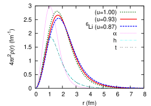
Figure 1: Point-matter densities of ⁶Li with different values of the $u$ parameter in the MN potential. The densities of $\alpha$, $h$, and $t$ with $u=0.93$ are also plotted for comparison.

Figure 1 plots the point-matter densities of ⁶Li with different values of the $u$ parameter. The nuclear surface slightly extends with decreasing the odd-wave strength or the $u$ parameter. Peak positions are located in the range 1.6-1.7 fm and their magnitude become half at about 2.7-2.8 fm. We also plot the densities of $\alpha$, $h$, and $t$ with $u=0.93$. The calculated binding energies of $h$ and $t$ are respectively $-$7.68 and $-$8.38 MeV for $u=1.00$. They also do not depend on the choice of the $u$ parameter. Only 0.01 MeV difference is obtained for decreasing $u$ to $0.93$ and $0.87$. The peak of the density of $\alpha$ is at about 1 fm, showing the sharper distribution as compared to that of ⁶Li. The peak position of $h$ and $t$ are almost the same as that of ⁴He but the half-density positions are somewhat larger than that of ⁴He due to the weaker binding.

The ⁶Li nucleus is known to have developed $\alpha$ cluster structure and is well described with an $\alpha+p+n$ three-body model Horiuchi07 having significant amount of the $\alpha+d$ component Watanabe15 ; Kawamura19 . As a measure of the clustering degrees-of-freedom, we also show the spectroscopic factor of the $\alpha+d$ configuration. The probability of finding the two-cluster ($a$ and $b$) configurations in the ⁶Li wave function is defined by

$$S_{ab}^{2} =\left|\left<\left.\Psi^{(a)}\Psi^{(b)}\right|\Psi^{(6)}_{JM_{J}}(E)\right>\right|^{2},$$ (9)

where $\Psi^{(a)}$, $\Psi^{(b)}$, and $\Psi^{(6)}_{JM_{J}}(E)$ are the ground-state wave functions of nuclei $a$, $b$, and ⁶Li with energy $E$, respectively. The relative wave function on the coordinate between the cm of the nuclei $a$ and $b$ is integrated out. Details of this evaluation is given in Appendix. We calculate the $S_{\alpha d}^{2}$ values ($a=\alpha$, $b=d)$ for the ground-state wave functions which are listed in Table 1. The $S_{\alpha d}^{2}$ values are found being large 0.86–0.88 for all the values of the $u$ parameter, which is consistent with the value obtained with the variational Monte Carlo calculation, 0.84 Forest96 . The $\alpha+d$ cluster structure is somewhat distorted by the $NN$ interaction and the Pauli principle. In fact, the $S_{\alpha d}^{2}$ value slightly increases by adding the repulsive $\alpha$-nucleon interaction with $u=0.93$ and $0.87$. Though $S_{\alpha d}^{2}$ values are large, no bound state in the ⁶Li system is obtained only with the $\alpha+d$ configurations with a relative $s$-wave. Inclusion of those distorted configurations is essential to get binding in the six-nucleon system.

III.2 Final-state wave functions

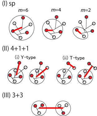
Figure 2: Schematic figures of the basis functions for the final-state wave functions. Colored and uncolored small circles represent protons and neutrons, respectively. Thick lines indicate the coordinates excited by the $E1$ operator. See text for exact definitions.

In this subsection, we explain how to construct the final-state wave functions excited by the $E1$ operator. We follow almost the same prescription as given in Refs. Horiuchi12 ; Horiuchi13 ; Mikami14 but are extended for adopting to the ⁶Li case. The ground-state wave function with $J^{\pi}=1^{+}$ is excited by the $E1$ operator. Since the operator does not change the spin of the initial state $S=1$, the orbital angular momentum of the final state should be $L=1$ and thus $J^{\pi}=0^{-},1^{-}$, and $2^{-}$ states need to be considered. In this paper, we did not include the spin-orbit interaction. These states are energetically degenerate that only its multipolarity is different.

We expand the final-state wave function in a large number of the correlated Gaussian basis functions of Eq. (3). To incorporate the complicated six-body correlations efficiently, physically important configurations are selected and categorized into the three types below: (I) Single-particle (sp) excitation, (II) 4+1+1 cluster, and (III) 3+3 cluster configurations. All these configurations are again expressed by the same functional form as of Eq. (3) with appropriate coordinate transformations.

The configurations of type (I) is based on the idea that the $E1$ operator excites one coordinate in the ground-state wave function and these configurations are further subcategorized into three channels which will be explained later in this paragraph. The resulting coherent states are important to satisfy the $E1$ sumrule Horiuchi12 . The configurations of type (I) are constructed by using the basis set of the ground-state wave function of ⁶Li by multiplying additional angular momentum $L=1$ as

$$\Phi_{JM_{J},i}^{{\rm(sp,}n)}=\mathcal{A}\left[\Phi_{1,i}^{(6)}(123456)\mathcal{Y}_{1}(\bm{r}_{1}-\bm{x}_{\rm cm}^{(m)})\right]_{JM_{J}},$$ (10)

where $\Phi_{1,i}^{(6)}$ is the $i$th basis $(i=1,\dots,600)$ of the ground-state wave function of ⁶Li. The coordinate $\bm{r}_{1}$ denotes the single-particle coordinate of a proton. As a first choice, we take the coordinate of one proton measured from the cm of the system ($m=6$). Considering that ⁶Li has large $S_{\alpha d}^{2}$ component $\sim$0.9, we include the additional sp basis sets that the four- and two-nucleon subsystems are excited by the $E1$ operator (the channels with $m=4$ and 2). Finally, the total number of the basis of the type (I) is 1800 including the channels with $m=6,4$, and 2.

The configurations of types (II) and (III) explicitly take care of the cluster configurations of $\alpha+p+n$ and $h+t$, which correspond to the two lowest thresholds, 3.7 and 15.8 MeV Tilley02 , respectively. They are expected to be important for describing the low-lying ($\lesssim$16 MeV) and intermediate energies ($\gtrsim$16 MeV).

The configurations of type (II) are defined in the following

$$\Phi_{JM_{J},ijk}^{(411,l)}=\mathcal{A}\left\{\Phi_{0,i}^{(4)}(1234)\exp\left(-\frac{1}{2}\tilde{\bm{y}}B^{(jk)}\bm{y}\right)\right.$$

$$\times\left.\left[\mathcal{Y}_{1}(\bm{y}_{l}^{({\rm X})})\left[\chi_{\frac{1}{2}}(5)\chi_{\frac{1}{2}}(6)\right]_{S_{56}}\right]_{JM_{J}}\eta_{\frac{1}{2},-\frac{1}{2}}(5)\eta_{\frac{1}{2},\frac{1}{2}}(6)\right\},$$ (11)

where $\Phi_{0,i}^{(4)}$ is the $i$th basis that gives the ground-state energy of ⁴He with the full set of these basis functions. The following two types of relative coordinates are considered:
(i) Y-type

$$\bm{y}_{1}^{({\rm Y})}=\bm{r}_{5}-\bm{x}_{\rm cm}^{(4)},\quad\bm{y}_{2}^{({\rm Y})}=\bm{r}_{6}-\frac{\bm{r}_{5}+4\bm{x}_{\rm cm}^{(4)}}{5},$$ (12)

(ii) T-type

$$\bm{y}_{1}^{({\rm T})}=\bm{r}_{6}-\bm{r}_{5},\quad\bm{y}_{2}^{({\rm T})}=\frac{\bm{r}_{5}+\bm{r}_{6}}{2}-\bm{x}_{\rm cm}^{(4)}.$$ (13)

These configurations are essential for describing the two valence nucleon motion around the $\alpha$ core which will be important, especially, in the low-lying energies. For the Y-(T-)type channel, we assume that both of the $\bm{y}_{1}^{({\rm X})}$ and $\bm{y}_{2}^{({\rm X})}$ coordinates are initially in $p$($s$)-wave and the one coordinate is excited to $s$($p$)-wave state. We consider either $\bm{y}_{1}^{({\rm X})}$ or $\bm{y}_{2}^{({\rm X})}$ in each coordinate set is excited by the $E1$ operator, that is, the basis set with $l=1$ and 2 are independently included respectively for (i) and (ii). The relative wave functions of the valence nucleons are expanded with several Gaussian functions covering from short to far distances, that is, the diagonal matrix elements of a $2\times 2$ matrix $B$, e.g., $B_{11}=1/b_{11}^{2}$, are chosen by a geometric progression with 18 and 15 basis ranging from 0.1 fm to 22 fm for the $\bm{y}_{1}^{({\rm X})}$ and $\bm{y}_{2}^{({\rm X})}$ coordinates, respectively. For practical computations, we truncate the number of the basis function of the four nucleon subsystem, $\Phi_{0,i}^{(4)}$, with 15 basis. Though the energy loss of this $\alpha$ particle is tiny in which only 0.3 MeV difference from the full model space calculation is found, it drastically reduces the total number of the basis functions.

The configurations of type (III) are defined as

$$\Phi_{JM_{J},ijk}^{(33)} =\mathcal{A}\left\{\left[\left[\Phi_{\frac{1}{2},i}^{(3)}(123)\Phi_{\frac{1}{2},j}^{(3)}(456)\right]_{J_{3}}\right.\right.$$

$$\times\left.\left.\exp\left(-\frac{1}{2}b_{k}z^{2}\right)\mathcal{Y}_{1}(\bm{z})\right]_{JM_{J}}\right\}$$ (14)

with

$$\bm{z}=\frac{\bm{r}_{1}+\bm{r}_{2}+\bm{r}_{3}}{3}-\frac{\bm{r}_{4}+\bm{r}_{5}+\bm{r}_{6}}{3},$$ (15)

where $\Phi_{\frac{1}{2},i}^{(3)}(123)$ and $\Phi_{\frac{1}{2},j}^{(3)}(456)$ are the $i$th and $j$th bases that give respectively the ground-state energies of ³He and ³H with the full set of these basis functions. These configurations describe the model space that directly excites the $h+t$ cluster degrees-of-freedom imprinted on the ground-wave function of ⁶Li ($S^{2}_{ht}\sim 0.4)$. The relative wave function for the coordinate $\bm{z}$ is expanded by 10 Gaussian functions with $p$-wave to reduce the computational cost. We also truncate the total number of basis functions for the three-nucleon subsystems by 7 bases resulting in only 0.2 MeV energy loss in these $h$ and $t$ particles.

Figure 2 shows schematic figures of the sets of the basis functions explained above. Circles and thick line in red indicate the protons and the coordinate excited by the $E1$ operator, respectively. Note that we include all the basis states for each subsystem independently. The final-state wave functions are not restricted the subsystems being the ground state but the excitations and distortion of ⁶Li, $\alpha$, $h$, and $t$ are included through the coupling of the pseudo excited states of those nuclear systems. The number of bases included in this calculation is 1800, 16200, and 490 for the configurations of types (I), (II), and (III), respectively. We diagonalize the Hamiltonian including all the configurations with 18490 basis functions and find $\sim 2\times 10^{3}$ states below the excitation energy of 100 MeV.

IV Results and discussions

IV.1 Electric-dipole transitions and nuclear clustering

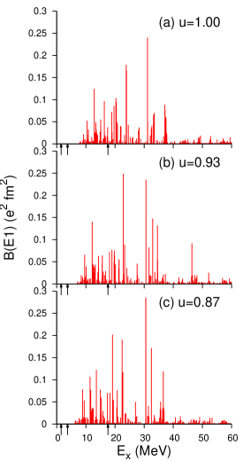
Figure 3: Electric-dipole strengths of ⁶Li with the full model space with (a) $u=1.00$, (b) 0.93, and (c) 0.87. Arrows indicate the theoretical $\alpha+d$, $\alpha+p+n$, and $h+t$ thresholds from left to right, respectively.

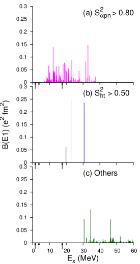
Figure 4: Electric-dipole strengths of ⁶Li with the full model space with $u=0.93$ categorized by the amount of the spectroscopic factors into three: (a) $S_{\alpha pn}^{2}>0.80$, (b) $S_{ht}^{2}>0.5$, and (c) neither (a) nor (b). See text for details. Arrows indicate the theoretical $\alpha+d$, $\alpha+p+n$, and $h+t$ thresholds from left to right, respectively.

Figure 3 plots the $E1$ transition strengths obtained with the full model space that includes the configurations of types (I)–(III) described in the previous section with different values of the $u$ parameter as a function of the excitation energy, $E_{x}=E_{f}-E_{0}$. For all these $u$ values, we see several large $B(E1)$ values in the low ($E_{x}\lesssim 16$ MeV), intermediate ($E_{x}\sim 16$–30 MeV), and high ($E_{x}\gtrsim 30$ MeV) energy regions. Though there is little quantitative difference among these three different cases up to $E_{x}\sim$40 MeV, hereafter we discuss the results with $u=0.93$ unless otherwise mentioned.

The structure of those peaks becomes more transparent by categorizing those states with respect to the spectroscopic factors of the $\alpha+p+n$ configuration

$$S_{\alpha pn}^{2}=\left.\left|\left<\Psi^{(\alpha)}\Psi^{(p)}\Psi^{(n)}\right.|\Psi^{(6)}_{JM_{J}}(E)\right>\right|^{2},$$ (16)

where $\Psi^{(\alpha)}$ is the ground-state wave function of ⁴He, and $\Psi^{(p)}$ ($\Psi^{(n)}$) is the proton (neutron) wave function. All the relative coordinates between clusters, spins and isospins are integrated out. Details about the evaluation are given in Appendix. Note that $S^{2}_{\alpha d}$ is a subset of $S_{\alpha pn}^{2}$ but the states with large $S^{2}_{\alpha d}$ value does not contribute to the $E1$ transition. No $E1$ transition occurs from the ground state to those states because their total isospins are almost 0.

Panel (a) of Fig. 4 displays the transition strengths to the states with $S_{\alpha pn}^{2}>0.80$. We find that the $E1$ transition strengths distribute in ranges from 10 to 40 MeV and that most of the low-lying states below 20 MeV have a large $\alpha+p+n$ cluster component, which is consistent by reminding the facts that the lowest $h+t$ threshold is 15.8 MeV Tilley02 .

Panel (b) of Fig. 4 shows the $E1$ strengths with $S_{ht}^{2}>0.50$. Three large $E1$ strengths appear after the $h+t$ threshold opens. We find that these peak structures are robust, and their positions and strengths do not depend much on the values of the $u$ parameter. The first two structures may correspond to the observed $J^{\pi}=2^{-}$ levels at $E_{x}=17.98$ and 26.59 MeV with the $h+t$ decay widths of 3.0 and 8.7 MeV, respectively Tilley02 .

The other strengths which cannot be categorized into the above two conditions are plotted in the panel (c) of Fig. 4. They appear beyond 30 MeV and some prominent $E1$ strengths are found between 30 and 40 MeV. In this energy region, the all particle thresholds are open. Various configurations can couple with each other. We will discuss more details in Sec. IV.3.

Table 2: Excitation energy ($E_{x}$), reduced electric-dipole transition probability [$B(E1)$] in unit of $e^{2}$fm², and $\alpha+p+n$ ($S_{\alpha pn}^{2}$) and $h+t$ ($S_{ht}^{2}$) spectroscopic factors of ⁶Li with $u=0.93$. Note that two prominent strengths with different configurations appear at $E_{x}=30.6$ MeV.

$E_{x}$(MeV)	$B(E1)$	$S_{\alpha pn}^{2}$	$S_{ht}^{2}$
9.6	0.066	0.999	0.000
12.1	0.140	0.999	0.011
14.3	0.063	0.997	0.000
15.7	0.064	0.999	0.010
18.9	0.077	0.991	0.004
19.8	0.075	0.994	0.003
22.8	0.249	0.113	0.850
23.3	0.089	0.963	0.003
30.6	0.236	0.264	0.533
30.6	0.095	0.780	0.158
33.0	0.148	0.962	0.005
34.6	0.132	0.195	0.019

We discuss the structure of the states with large $E1$ strengths. For quantitative discussions, we list, in Table 2, $E_{x}$, $B(E1)$, $S_{\alpha pn}^{2}$, and $S_{ht}^{2}$ of the states giving four largest $B(E1)$ values in the low-, intermediate-, and high-energy regions with $u=0.93$. In the low energy regions ($E_{x}\lesssim$16 MeV) below the $h+t$ threshold, all the states have large $S_{\alpha pn}^{2}$ values being almost unity, whereas their $S_{ht}^{2}$ values are almost zero.

In the intermediate energy regions around 20 MeV where $\alpha$-cluster can be energetically possible to break, although most of the states still have large $S_{\alpha pn}^{2}$ values, the state at $E_{x}=22.8$ MeV have a small $S_{\alpha pn}^{2}$ value in which the $\alpha$ cluster in the six-nucleon system is strongly distorted. This state is dominated by the $h+t$ configuration having the large $S_{ht}^{2}$ value 0.850.

In the high energy regions beyond $\sim$30 MeV where all the particle thresholds are open, various structures are found: Mixture of $\alpha+p+n$ and $h+t$ components at $E_{x}=30.6$ MeV, almost pure $\alpha+p+n$ component at $E_{x}=33.0$ MeV, and neither $\alpha+p+n$ nor $h+t$ components at $E_{x}=34.6$ MeV.

We have shown the $E1$ strength distributions with the full model space including the breaking and polarization of the clusters in ⁶Li. To make the role of these effects clearer, we calculate the $E1$ transition strengths only with the $\alpha+p+n$ and $h+t$ configurations that are respectively constructed by the diagonalization of the following basis functions

$$\Phi_{JM_{J},jk}^{(\alpha pn),m} =\sum_{i}C_{i}^{(\alpha)}\Phi_{JM_{J},ijk}^{411,m},$$ (17)

$$\Phi_{JM_{J},k}^{(ht)} =\sum_{i,j}C_{i}^{(h)}C_{j}^{(t)}\Phi_{JM_{J},ijk}^{(33)},$$ (18)

where $C_{i}^{(x)}$ are a set of the coefficients that give the ground-state wave function of a cluster $x(=h$, $t$, and $\alpha$). Figure 5 plots the transition strengths only with the $\alpha+p+n$ and $h+t$ final-state configurations. As expected the transition strengths only with the $\alpha+p+n$ configurations below 30 MeV are similar to the results displayed in the panel (a) of Fig. 4 where the $S_{\alpha pn}^{2}$ values are large. We only find three significant strengths with the $h+t$ configurations and the positions of the two lowest prominent peaks at $E_{x}=20.0$ and 23.9 MeV remain unchanged with the full model space calculations, while the most prominent peak at $E_{x}=36.4$ MeV split into small strengths in the full model space calculation as shown in the panel (b) of Fig. 3. We find the state has relatively large square overlap with the $\alpha+p+n$ configuration (0.281), leading to the level splitting due to the channel coupling.

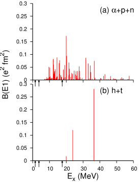
Figure 5: Electric-dipole strengths only with (a) $\alpha+p+n$ and (b) $h+t$ final-state configurations. Arrows indicate the theoretical $\alpha+d$, $\alpha+p+n$, and $h+t$ thresholds from left to right, respectively.

IV.2 Non-energy weighted sumrule

Here we discuss the impact of the clustering configurations on the $E1$ sumrule. The non-energy-weighted sumrule (NEWSR) can be evaluated by

$$\sum_{E_{f}}B(E1,E_{f})=e^{2}\left(Z^{2}r_{p}^{2}-\frac{Z(Z-1)}{2}r_{pp}^{2}\right).$$ (19)

We obtain 4.49 $e^{2}$fm² as a total sum of the $E1$ transition strengths with the full model space. The NEWSR is fully satisfied, that is, 99.6% of the right-hand-side of Eq. (19) is fulfilled in the present model space. To quantify the importance of the $\alpha$ clustering, we calculate the left-hand-side equation only with the $\alpha+p+n$ configuration defined in Eq. (17) and the value is 2.45 $e^{2}$fm², satisfying 55% of the total sumrule value. Figure 6 compares the cumulative sum of ⁶Li of the $E1$ strengths with the full model space as well as the ones only with the $\alpha+p+n$ configurations. To get the sumrule satisfied, say 80%, the cumulative sum with the full model space needs to integrate up to about 45 MeV, whereas the most of the important configurations with the $\alpha+p+n$ configuration are exhausted at 33 MeV where its cumulative sum exceeds 80% of its total sum. We find that the configurations other than the $\alpha+p+n$ configurations are also important in such low-lying regions below $\sim$20 MeV even the $h+t$ threshold does not open. They are used to describe the polarization of the clusters through the coupling of those cluster configurations. The difference between the cumulative sum of the full model space and $\alpha+p+n$ are 30% at 10 MeV and the difference becomes large as the incident energy increases. We also display in Fig. 6 the cumulative sum of the transition strengths with the mixing of $\alpha+p+n$ and $h+t$ configurations defined respectively in Eqs. (17) and (18). The $h+t$ configurations play a role beyond $\sim 20$ MeV after opening the $h+t$ threshold and improve the NEWSR value by 8%. However, it is not enough to explain all the needed configurations included in the strengths with the full model space. In the higher energies, the breaking of these cluster configurations becomes more important as various configurations can contribute to the $E1$ transitions.

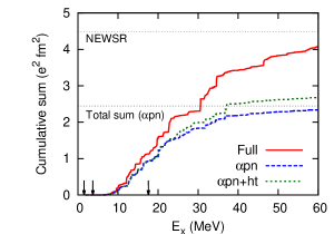
Figure 6: Cumulative sum of the $E1$ transition strengths of ⁶Li with the full model space, $\alpha+p+n$, and $(\alpha+p+n)+(h+t)$ configurations with $u=0.93$. The non-energy-weighted sumrule (NEWSR) value and the total sum of the $E1$ strengths only with the $\alpha+p+n$ configurations are plotted as thin dotted lines for comparison. See text for details. Arrows indicate the theoretical $\alpha+d$, $\alpha+p+n$ and $h+t$ thresholds from left to right, respectively.

IV.3 Structure of the electric-dipole excitation

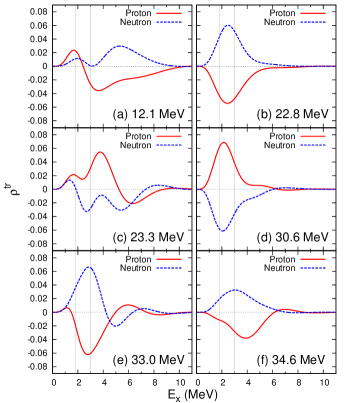
Figure 7: Transition densities of ⁶Li with the excitation energy of (a) 12.1, (b) 22.8, (c) 23.3, (d) 30.6, (e) 33.0, and (f) 34.6 MeV selected from Table 2. See text for details. Note that left panels plot the transition densities with the states having large $S_{\alpha pn}^{2}\sim 1$. Vertical thin lines indicate theoretical nuclear radii, $\sqrt{\frac{5}{3}}r_{m}$, with $r_{m}=1.41$ and 2.33 fm for ⁴He and ⁶Li, respectively.

Let us discuss the spatial structure of the $E1$ transitions. For this purpose, we calculate the transition densities of ⁶Li for the analysis of the $E1$ transition mode Mikami14

$$\rho^{\rm tr}_{p/n}(r)=\sum_{i\in p/n}\left<\Psi_{J_{f}}^{(6)}\right\|\mathcal{Y}_{1}(\bm{r}_{i}-\bm{x}_{6})\delta(|\bm{r}_{i}-\bm{x}_{6}|-r)\left\|\Psi_{J_{0}}^{(6)}\right>,$$ (20)

for proton and neutron. This quantities represent the spatial distributions of the proton and neutron transition matrices reminding that the $E1$ transition matrix can be obtained with

$$\left<\Psi_{J_{f}}^{(6)}\right\|\mathcal{M}(E1)\left\|\Psi_{J_{0}}^{(6)}\right>=e\sqrt{\frac{4\pi}{3}}\int_{0}^{\infty}dr\,\rho^{\rm tr}_{p}(r).$$ (21)

We discuss the transition densities of ⁶Li to the selected states that show some characteristic behaviors. Figure 7 plots the transition densities for proton and neutron that correspond to the prominent $B(E1)$ peaks with $B(E1)>0.1$ $e^{2}$fm². At the low energy (a) $E_{x}=12.1$ MeV, we see the in-phase transition below the ⁶Li radius and the out-of-phase transitions occur outside the nuclear surface. This characteristic transition can be interpreted as the GDR-like or Goldhaber-Teller-(GT)-dipole type oscillation Goldhaber48 of the valence proton and neutron around the core ($\alpha$). In fact, the state have large $S_{\alpha pn}^{2}$ value as listed in Table 2. This type of “soft” GT-dipole mode is very unique in ⁶Li and differs from the soft-dipole mode expected in ⁶He that the oscillation between the valence two neutrons against the core. We note that the $E1$ transitions to $\alpha+d$ is almost forbidden because the $E1$ operator is isovector and the ground state of ⁶Li is almost pure $T=0$ state though small mixture of the other total isospin state is included. Actually, the $S_{\alpha d}^{2}$ value for this state is 0.02. Studying the low-lying $E1$ excitations of ⁶Li is the ideal example that the soft GT-dipole mode dominates.

In the energy regions where the $h+t$ threshold opens, we see clear out-of-phase transitions in all regions at (b) $E_{x}=22.8$ MeV which is typical for the GDR mode. As $S_{ht}^{2}$ is large $>0.8$, this behavior comes from the $E1$ excitation of the relative motion between the $h$ and $t$ clusters. Peak positions are at $\sim$2 fm located at the sum of the peak positions of the density distributions of ³H and ³He displayed in Fig. 1. Such cluster GT-dipole modes can appear in any nuclear systems but its emergence depends on the location of the cluster threshold. In light nuclei, since the cluster threshold becomes low, the cluster GT dipole modes can appear in the lower-lying regions. For the ⁷Li case, the $\alpha+t$ threshold is lowest (2.47 MeV Tilley02 ), it differs from the case of ⁶Li, the cluster GT-dipole mode is expected to appear in the lowest energy regions.

We also find large $B(E1)$ value at almost the same energy (c) $E_{x}=23.3$ MeV. Similarly to the transition density at (a) $E_{x}=12.1$ MeV, we see the in-phase transition below the ⁶Li radius but more oscillations in the out-of-phase transition appear in the outside of the nuclear surface. Since this state has large $S_{\alpha pn}^{2}$ value listed in Table 2, this state can be interpreted as a vibrational excitation of the soft GT-dipole mode. The transition densities with (e) $E_{x}=33.0$ shows the similar character having more oscillations.

At (d) $E_{x}=30.6$ MeV, this shows the out-of-phase transition in all regions. Since the peak position is almost the same as that of (b) $E_{x}=23.3$ MeV and has large mixture of $h+t$ configurations $\sim 0.5$ listed in Table 2, this state can be regarded as a vibrational excitation of of the state with (c) $E_{x}=23.3$ MeV which exhibits the $h+t$ clustering.

Finally, the state with (f) $E_{x}=34.6$ MeV shows also the out-of-phase transition in all regions but the peak positions are located outside of the nuclear surface showing totally different structure from that of the $h+t$ oscillation. Neither $S_{\alpha pn}^{2}$ nor $S_{ht}^{2}$ is large as listed in Table 2. This state can be regarded as having the typical GDR structure that the protons and neutrons oscillate opposite to each other Goldhaber48 .

To strengthen the interpretations given above, we calculate the transition densities with the final-state wave functions only with the $\alpha+p+n$ and $h+t$ configurations. These transition strengths with the limited model spaces were already given in Fig. 5. The transition densities with the $\alpha+p+n$ configuration that give the three largest $B(E1)$ strengths for each configuration are shown in the panels (a), (c), and (e) of Fig. 8. These almost explain the characteristics behavior of the transition densities of the states with large $S_{\alpha pn}^{2}$, that are, the soft GT-dipole modes. All the transition densities have in-phase transitions inside about the nuclear radius and out-of-phase transitions beyond the surface. It is interesting to note that the nodal or oscillatory behavior in the in-phase regions of the transition densities at around the radius of the $\alpha$ particle. This is due to the Pauli principle between the core and valence nucleon. As we see in the transition densities of ⁶He, the nodal behavior of the transition density can only be seen in the neutron transition Mikami14 .

We also plot, in the panels (b) and (d) of Fig. 8, the transition densities only with the $h+t$ configurations for the states giving the two highest $E1$ strengths. They show typical GDR behavior and peak positions are at around the nuclear surface which explains the behavior of the transition densities of (b) and (d) of Fig. 7. In this restricted model space, we do not obtain the similar transition densities to the state with $E_{x}=34.6$ MeV, implying that these clusters are strongly distorted as was shown in the GDR mode at $E_{x}=32.9$ MeV in ⁶He Mikami14 .

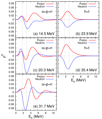
Figure 8: Transition densities to the states that give the prominent $E1$ strength only with the restricted model spaces: The $\alpha+p+n$ final-state configurations at (a) $E_{x}=14.5$, (c) 20.3, and (e) 31.7 MeV; and the $h+t$ final-state configurations at (b) $E_{x}=23.9$ and (d) 35.4 MeV. See text for details. Vertical thin lines indicate theoretical nuclear radii, $\sqrt{\frac{5}{3}}r_{m}$, of ⁴He and ⁶Li, respectively.

In summary, various types of the $E1$ excitations of ⁶Li can be classified by focusing on the nuclear clustering. The panels (a), (c), and (e) of Fig. 7 have the same characteristics that the in-phase transition below the ⁶Li radius due to the $\alpha$ clustering and out-of-phase transitions of the valence nucleons beyond the nuclear surface (Soft GT-dipole mode). The figures (b), (d), and (f) of Fig. 7 show the out-of-phase transition in all regions: The excitation modes of (b) and (d) are originated from the oscillations between $h$ and $t$ clusters (Cluster GT-dipole mode), and (f) is the typical GDR oscillation that protons and neutrons oscillate opposite to each other (GT-dipole mode).

IV.4 Photoabsorption cross sections

The total photoabsorption cross section is calculated by using the formula RS

$$\sigma_{\gamma}(E_{\gamma})=\frac{4\pi^{2}}{\hbar c}E_{\gamma}\frac{1}{3}\frac{dB(E1,E_{\gamma})}{dE},$$ (22)

The continuum states are discretized in this calculation. For a practical reason, they are often smeared by the Lorentzian functions $dB(E1,E)/dE=\frac{\Gamma}{2\pi}\sum_{\nu}B(E1,E_{\nu})/[(E-E_{\nu}-E_{0})^{2}+(\Gamma/2)^{2}]$, using a certain $\Gamma$ value as a free parameter Pinilla11 . To compare with the recent experiment, we fix the width parameter so as to reproduce the total sum of the experimental cross sections of Ref. Yamagata17 . However, the energy-independent width does not work that results in the unphysically large decay width $\sim$40 MeV. Thus, we use the energy dependent decay width that starts from the the lowest threshold: $\Gamma(E)=[E-E(\alpha+d)]\tan 2\theta$, where $E(\alpha+d)$ is the $\alpha+d$ threshold energy. The $\theta$ value is determined to $27^{\circ}$ which reproduces the the total sum of the cross sections of Ref. Yamagata17 .

Figure 9 compares the calculated and experimental photoabsorption cross sections of ⁶Li. Most of the experimental data are the cross sections for the ⁶Li($\gamma,n$) reactions but the ⁶Li($\gamma,2n$) and ⁶Li($\gamma,3n$) cross sections are negligibly small in this energy region Yamagata17 . In the calculated total photoabsorption cross sections, only a single-peak structure is found. We remark that Ref. Bacca02 ; Bacca04 also predicted a broad single-peak structure at around 20 MeV for the total photoabsorption cross sections of ⁶Li with the six-body calculation. The results are almost identical for all $u$ parameters due to large smearing width $\Gamma(E)$. Though all fine structures are smeared out, the cross section values are quantitatively consistent with the measured cross sections considering that the measured values are very much scattered. For the quantitative comparison to the measured cross sections, it is necessary to describe the six-body continuum states appropriately with the aid of, e.g., the complex scaling method Moiseyev98 ; Aoyama06 as well as the improvement of the nuclear interaction, although they are involved.

Let us compare the interpretation given in Refs. Costa63 ; Yamagata17 and our findings. The measured cross sections of Ref. Yamagata17 show the two-peak structure and their interpretation on the two-peak structure was that, the low-lying ($E_{\gamma}\lesssim 20$ MeV) peak comes from the typical GDR transition mode of ⁶Li and the higher peak (from $\sim 30$ to $\sim 40$ MeV) corresponds to the GDR of the $\alpha$ cluster in ⁶Li. Contrary to that interpretation, we see the typical GDR or GT mode appears in the higher-lying energy regions around 35 MeV, where the $\alpha$ cluster is strongly distorted. In Ref. Costa63 , the lower peak is interpreted as the disintegration to the $\alpha+p+n$ channels, whereas the higher peak is the GDR of ⁶Li due to the disintegration of the $\alpha$ core. From the theoretical point of view, it is difficult to say whether this GDR mode is the GDR of the $\alpha$ cluster in ⁶Li or not in the high energy regions because identical fermions cannot be distinguished where they belong to. In our interpretation, in the low-lying energy regions below the $h+t$ threshold (15.8 MeV), the soft GT-dipole transitions dominate that the out-of-phase transition between the valence nucleons around the $\alpha$ cluster, which is consistent with the interpretation given in Ref. Costa63 for the lower energy peak. This can be realized as all the spectroscopic factors, $S_{\alpha pn}^{2}$, of the final states in this energy regions are almost unity. It is known that the excitation energy of the GDR is inversely proportional to the nuclear radius. According to the systematics of the GDR energy RS , this low-lying energy region corresponds to the GDR energies of $A\sim 200$ nuclei. Therefore, it is natural to interpret that the typical excitation mode in this energy region is the GT mode of the valence nucleons around the tightly bound $\alpha$ core, whereas the typical GDR mode of ⁶Li suggested in Ref. Yamagata17 is unlikely, reminding that the ⁶Li radius is about one half of the radii of the $A\sim 200$ nuclei Angeli13 . In the intermediate energies from $\sim 20$ to $\sim 30$ MeV just between the low and high-lying peaks of ⁶Li, the prominent $h+t$ cluster GT-dipole mode appears, which is consistent with the interpretation given in Ref. Costa63 for the higher energy peak. As summarized at the end of the previous subsection, the emergence of these various excitation modes can simply be recognized by the threshold energies, the Ikeda threshold rule Ikeda68 .

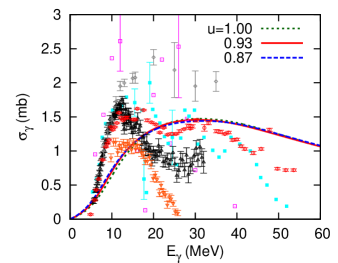
Figure 9: Comparison of the photoabsorption cross sections of ⁶Li. Experimental ⁶Li$(\gamma,n)$ data are plotted as open rectangles Costa63 , closed rectangles Bazhanov65 , open triangles Berman65 , inverted open triangles Denisov67 , and diamonds Wurtz14 . Since they are unavailable, most of error bars of the experimental data in Refs. Costa63 ; Denisov67 are not plotted. Open circles stand for the ⁶Li$(\gamma,n)+^{6}$Li$(\gamma,2n)+^{6}$Li$(\gamma,3n)$ data taken from Ref.Yamagata17 .

IV.5 Isoscalar dipole transitions

Here we discuss an other operator to discuss more details on the transition densities. The compressive isoscalar dipole (IS1) operator Stringari82 is defined by

$$\mathcal{M}({\rm IS}1)=\sum_{i}(\bm{r}_{i}-\bm{x}_{N})^{2}\mathcal{Y}_{1\mu}(\bm{r}_{i}-\bm{x}_{N}).$$ (23)

The transition matrix of IS1 can be calculated by using the relation: $\int_{0}^{\infty}dr\,r^{2}\left(\rho_{p}^{\rm tr}+\rho_{n}^{\rm tr}\right)$. The IS1 transitions have recently been intensively discussed because it has of particular importance to study the cluster structure (See recent theoretical and experimental papers Chiba17 ; Enyo17 ; Adachi18 and references therein).

Figure 10 plots the IS1 strength distributions as a function of the excitation energies. We see some prominent strengths below 5 MeV having the isoscalar nature possibly by the $\alpha+d$ continuum, which cannot be excited by the $E1$ operator that only has the isovector term. In fact, the $S_{\alpha d}^{2}$ values of those states are found to be almost unity and the transition densities of the state with the most prominent IS1 peak at $E_{x}=3.3$ MeV shows in-phase transition in all regions. Beyond 5 MeV, the IS1 strengths drop suddenly and very small strengths appear in the higher energy regions. The most of the IS1 strengths are exhausted by the transitions to the $\alpha+d$ states below 5 MeV. In case of ⁶He Mikami14 , since the low-lying soft-dipole mode is dominated by the surface excitation of the valence neutrons, several IS1 strengths appear at the low-lying regions. Contrary to the ⁶He case, the states with all the prominent $E1$ strengths have the out-of-phase excitation character. The IS1 transition matrix which is obtained by the sum of proton and neutron transition densities is strongly canceled out in such excitation modes where the out-of-phase transitions dominate. The contributions from the in-phase transition regions in the soft GT-dipole mode become small in the IS1 strengths due to the additional $r^{2}$ factor appearing in the IS1 operator. The strong suppression of the IS1 transition strengths can be the evidence that all the ⁶Li final states beyond 5 MeV are dominated by the out-of-phase transitions. We remark that similar transition strengths are observed in the proton inelastic scattering on ⁶Li Yamagata06 , although a proton probe can excite both the isoscalar and isovector components. The experimental confirmation using an isoscalar probe such as an $\alpha$ particle is desired to clarify the excitation mechanism of ⁶Li.

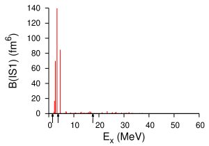
Figure 10: Isoscalar dipole strengths of ⁶Li as a function of the excitation energy. Arrows indicate the theoretical $\alpha+d$, $\alpha+p+n$ and $h+t$ thresholds from left to right, respectively.

V Conclusion

Motivated by the recent measurement of the photoabsorption cross sections of ⁶Li Yamagata17 , we have performed fully microscopic six-body calculations for the electric-dipole ($E1$) transition strengths. The ground-state wave function of ⁶Li was obtained precisely by using the correlated Gaussian (CG) functions with the stochastic variational method. The final-state wave functions populated by the $E1$ operator were expanded by a number of the CG functions including the explicit asymptotic cluster wave functions as well as their distorted configurations that are important to describe the complicated six-nucleon dynamics. Emergence of various excitation modes has been found through the analysis of the transition densities from the ground to final-state wave functions. The degrees of the clustering in those states have been quantified by evaluating the components of the $\alpha+p+n$ and $h+t$ clusters in the ⁶Li wave functions to understand the role of these cluster configurations in the $E1$ excitations.

Nuclear clustering plays a crucial role in explaining the $E1$ excitation mechanism of ⁶Li and its emergence strongly depends on the positions of the threshold energies. In the low energy regions below the $\alpha$ breaking or $h+t$ threshold energy $\lesssim 16$ MeV, we found that the $E1$ excitations are dominated by the “soft” dipole mode that exhibits the in-phase transitions of proton and neutron transition densities in the internal regions and the out-of-phase transitions beyond the nuclear surface. This can be interpreted as the out-of-phase oscillation between valence nucleons around the $\alpha$ cluster in ⁶Li [“soft” Goldhaber-Teller(GT)-dipole mode], which is a very unique excitation mode. After the $h+t$ thresholds open, the $h+t$ cluster mode appears showing the out-of-phase transition in all regions and they also compete with the vibrational excitation of the soft GT-dipole modes having the $\alpha+p+n$ structure. Beyond 30 MeV, where all decay channels open, $\alpha+p+n$ and $h+t$ and other possible channels can mix and compete and finally typical GDR mode appear in this energy regions.

These interpretations are different from the speculation given in Ref. Yamagata17 that the low-energy peak corresponds to the typical GDR of ⁶Li. From the present analysis, we found that the $E1$ transition strengths of the ⁶Li are dominated by the out-of-phase transitions of protons and neutrons in the surface regions from the low- to high-energy regions, which is in contrast to ⁶He where the neutron transition dominates at the low energy regions. This phase property can be verified by using an isoscaler probe such as $\alpha$ inelastic scattering measurement to confirm whether no prominent strength is found or not after the $\alpha+p+n$ threshold.

It is interesting to explore whether the soft GT mode appears in the low-lying energy regions of heavier nuclei. Since the excitation mode emerges from the out-of-phase transition of the proton and neutron of the $d$-cluster around the core in the initial ground-state wave function, the ground-state wave function should have a well-developed core plus $d$-cluster structure. The most probable candidate is ¹⁸F because the ground-state spin-parity is $1^{+}$ like ⁶Li and a ¹⁶O$+p+n$ cluster structure component can be large.

Also, as a natural extension of ⁶Li, a nucleus ⁷Li is worth studying Yamagata17 . Since the $\alpha+t$ threshold is the lowest (2.47 MeV), the cluster GT mode of $\alpha+t$ is expected to appear first, and then the other excitation modes appear with respect to the opening of the particle decay channels $\alpha+d+p$, $\alpha+p+p+n$, $t+h+n$, etc., in order.

These studies will serve as the universal understanding of the emergence of the nuclear clustering and reveal the excitation mechanism of nuclei through the $E1$ field, which is one of the most simplest probes of the nuclear structure.

Appendix A Calculation of the spectroscopic factors

As a measure of degrees of the clustering, we evaluate the spectroscopic factors, that are, the components of finding the $\alpha$, $\alpha+d$, and $h+t$ configurations in the wave function of ⁶Li. Eqs. (16) and (9), are respectively written more explicitly as

$$S_{\alpha pn}^{2} =\biggl{|}\iint d\bm{r}\,d\bm{r}^{\prime}\left<\Psi^{(\alpha)}\Psi^{(p)}\Psi^{(n)}\right|\biggr{.}$$

$$\biggl{.}\times\delta(\bm{y}_{1}-\bm{r})\delta(\bm{y}_{2}-\bm{r}^{\prime})\left|\Psi^{(6)}_{JM_{J}}(E)\right>\biggr{|}^{2},$$ (24)

$$S_{ht}^{2} =\left|\int d\bm{r}\left<\left.\Psi^{(h)}\Psi^{(t)}\delta(\bm{z}-\bm{r})\right|\Psi^{(6)}_{JM_{J}}(E)\right>\right|^{2}.$$ (25)

All the relative wave functions are integrated out by using the orthonormal basis $\sum_{lm}\phi_{l,i}(r)Y_{lm}(\hat{\bm{r}})$ constructed from a sufficient number of Gaussian functions, $r^{l}\exp(-ar^{2})$, as a complete set. Practically, we make the orthonormal basis sets by diagonalizing the relative wave functions used in the final-state wave function of types (II) and (III). More explicitly, we diagonalize the following overlap matrices using the coefficients of the bases that give the ground-state wave function of a nucleus $x$, $C_{i}^{(x)}$ for the $\alpha+p+n$ spectroscopic factor

$$B_{mn}^{(\alpha pn)}=\sum_{i,j}^{K_{4}}C_{i}^{(\alpha)}C_{j}^{(\alpha)}\left<\Phi_{JM_{J},im}^{(411,k)}\left|\Phi_{JM_{J},jn}^{(411,l)}\right.\right>$$ (26)

with $k$ and $l$ run for 1 and 2 corresponding to the Y- and T-types, respectively. We take $K_{4}=15$. In the end, the dimension of $B^{(\alpha pn)}$ is 1080. For the $h+t$ spectroscopic factors, we diagonalize the following overlap matrix

$$B_{mn}^{(ht)}=\sum_{i,j,k,l}^{K_{3}}C_{i}^{(h)}C_{j}^{(t)}C_{k}^{(h)}C_{l}^{(t)}\left<\Phi_{JM_{J},ijm}^{(33)}\left|\Phi_{JM_{J},kln}^{(33)}\right.\right>.$$ (27)

Finally, all the spectroscopic factors calculated in this paper are evaluated by the overlap matrix element of the correlated Gaussians SVM ; Suzuki08 . The same procedure is applied for the evaluation of the $\alpha+d$ spectroscopic factor as well.

References

- (1) K. Ikeda, N. Takigawa, H. Horiuchi, Prog. Theor. Phys. Suppl. E68, 464 (1968).
- (2) Y. Fujiwara, H. Horiuchi, K. Ikeda, M. Kamimura, K. Katō, Y. Suzuki, and E. Uegaki, Prog. Theor. Phys. Suppl. 68, 29 (1980).
- (3) F. Hoyle, Astrophys. J. Suppl. Ser. 1, 121 (1954).
- (4) M. Goldhaber and E. Teller, Phys. Rev. 74, 1046 (1948).
- (5) H. Steinwedel and J. H. D. Jensen, Z. Naturforsch. 5a, 413 (1950).
- (6) C. J. Horowitz and J. Piekarewicz, Phys. Rev. Lett. 86, 5647 (2001).
- (7) A. Tamii, I. Poltoratska, P. von Neumann-Cosel, Y. Fujita, T. Adachi, C. A. Bertulani, J. Carter, M. Dozono, H. Fujita et al., Phys. Rev. Lett. 107, 062502 (2011).
- (8) P. G. Hansen and B. Jonson, Europhys. Lett. 4, 409 (1987).
- (9) T. Yamazaki et al., A Draft Proposal for Japanese Hadron Project, p. 59 (1987) (in Japanese).
- (10) K. Ikeda, INS Report No. JHP-7 (1988) (in Japanese).
- (11) Y. Suzuki, K. Ikeda, and H. Sato, Prog. Theor. Phys. 83, 180 (1990).
- (12) D. Mikami, W. Horiuchi, and Y. Suzuki, Phys. Rev. C 89, 064303 (2014).
- (13) T. Inakura, W. Horiuchi, Y. Suzuki, and T. Nakatsukasa, Phys. Rev. C 89, 064316 (2014).
- (14) Y. Kanada-En’yo and Y. Shikata, Phys. Rev. C 95, 064319 (2017).
- (15) T. Yamagata, S. Nakayama, H. Akimune, and S. Miyamoto, Phys. Rev. C 95, 044307 (2017).
- (16) S. Costa, S. Ferroni, W. Wataghin, and R. Malvano, Phys. Lett. 4, 308 (1963).
- (17) W. Horiuchi and Y. Suzuki, Phys. Rev. C 76, 024311 (2007).
- (18) S. Watanabe, T. Matsumoto, K. Ogata, and M. Yahiro, Phys. Rev. C 92, 044611 (2015).
- (19) N. Kawamura and W. Horiuchi, Springer proceedings, in press.
- (20) D. R. Thompson, M. LeMere, and Y. C. Tang, Nucl. Phys. A 286, 53 (1977).
- (21) K. Varga and Y. Suzuki, Phys. Rev. C 52, 2885 (1995).
- (22) Y. Suzuki, W. Horiuchi, M. Orabi, and K. Arai, Few-Body Syst. 42, 33 (2008).
- (23) Y. Suzuki and K. Varga, Stochastic Variational Approach to Quantum-Mechanical Few-Body Problems, Lecture Notes in Physics, (Springer, Berlin, 1998), Vol. m54.
- (24) Y. Suzuki, J. Usukura, and K. Varga, J. Phys. B: At. Mol. Opt. Phys. 31, 31 (1998).
- (25) W. Horiuchi and Y. Suzuki, Phys. Rev. C 78, 034305 (2008).
- (26) W. Horiuchi and Y. Suzuki, Phys. Rev. C 89, 011304(R) (2014).
- (27) S. Ohnishi, W. Horiuchi, T. Hoshino, K. Miyahara, and T. Hyodo, Phys. Rev. C 95, 065202 (2017).
- (28) J. Mitroy, S. Bubin, W. Horiuchi, Y. Suzuki, L. Adamowicz, W. Cencek, K. Szalewicz, J. Komasa, D. Blume, and K. Varga, Rev. Mod. Phys. 85, 693 (2013).
- (29) Y. Suzuki and W. Horiuchi, Emergent phenomena in Atomic Nuclei from Large-scale Modeling: A Symmetry-Guided Perspective, Chapter 7, pp. 199-227 (World Scientific, Singapole, 2017).
- (30) D. R. Tilley, C. M. Cheves, J. L. Godwin, G. M. Hale, H. M. Hofmann et al., Nucl. Phys. A 708, 3 (2002).
- (31) I. Angeli and K. P. Marinova, Atomic Data and Nuclear Data Table 99, 69 (2013).
- (32) J. L. Forest, V. R. Pandharipande, S. C. Pieper, R. B. Wiringa, R. Schiavilla, and A. Arriaga, Phys. Rev. C 54, 646 (1996).
- (33) W. Horiuchi, Y. Suzuki, and K. Arai, Phys. Rev. C 85, 054002 (2012).
- (34) W. Horiuchi and Y. Suzuki, Phys. Rev. C 87, 034001 (2013).
- (35) P. Ring and P. Schuck, The Nuclear Many-Body Problem, Texts and Monographs in Physics (Springer, New York, Heidelberg, Berlin, 1980).
- (36) E. C. Pinilla, D. Baye, P. Descouvemont, W. Horiuchi, and Y. Suzuki, Nucl. Phys. A 865, 43 (2011).
- (37) E. B. Bazhanov, A. P. Komar, and A. V. Kulikov, Nucl. Phys. 68, 191 (1965).
- (38) B. L. Berman, R. L. Bramblett, J. T. Cadwell, R. R. Harvey, and S. C. Fultz, Phys. Rev. Lett. 15, 727 (1964).
- (39) V. P. Denisov, A. P. Komar, and L. A. Kul’chiskiy, Yad. Fiz. 5, 498 (1967).
- (40) W. A. Wurtz, R. E. Pywell, B. E. Norum, S. Kucuker, B. D. Sawatzky, H. R. Weller, S. Stave, and M. W. Ahmed, Phys. Rev. C 90, 014613 (2014).
- (41) S. Bacca, M. A. Marchisio, N. Barnea, W. Leidemann, and G. Orlandini, Phys. Rev. Lett. 89, 052502 (2002).
- (42) S. Bacca, N. Barnea, W. Leidemann, and G. Orlandini, Phys. Rev. C 69, 057001 (2004).
- (43) N. Moiseyev, Phys. Rep. 302, 221 (1998).
- (44) S. Aoyama, T. Myo, K. Katō, and K. Ikeda, Prog. Theor. Phys. 116, 1 (2006).
- (45) S. Stringari, Phys. Lett. B 108, 232 (1982).
- (46) Y. Chiba, Y. Taniguchi, and M. Kimura, Phys. Rev. C 95, 044328 (2017).
- (47) S. Adachi, T. Kawabata, K. Minomo, T. Kadoya, N. Yokota, H. Akimune, T. Baba, H. Fujimura, M. Fujiwara, et al., Phys. Rev. C 97, 014601 (2018).
- (48) T. Yamagata, N. Warashina, H. Akimune, S. Asaji, M. Fujiwara, M. B. Greenfield, H. Hashimoto, R. Hayami, T. Ishida et al., Phys. Rev. C 74, 014309 (2006).