Achieve Higher Efficiency at Maximum Power with Finite-time Quantum Otto Cycle

Abstract

The optimization of heat engines was intensively explored to achieve higher efficiency while maintaining the output power. However, most investigations were limited to few finite-time cycles, e.g. Carnot-like cycle, due to the complexity of the finite-time thermodynamics. In this paper, we propose a new class of finite-time engine with quantum Otto cycle, and demonstrate a higher achievable efficiency at maximum power. The current model can be widely utilized benefited from the general $\mathcal{C}/\tau^{2}$ scaling of extra work for finite-time adiabatic process with long control time $\tau$. We apply the current perturbation method to the quantum piston model and calculate the efficiency at maximum power, which is validated with exact solution.

I Introduction

The emergent studies of quantum thermodynamics (Campisi et al., 2011; Esposito et al., 2009; Maruyama et al., 2009; Strasberg et al., 2017; Vinjanampathy and Anders, 2016) have boosted the reminiscent investigation of heat engines into the microscopic level, especially on the optimizing performance (Curzon and Ahlborn, 1975; Geva and Kosloff, 1992; Esposito et al., 2010; Ryabov and Holubec, 2016) as well as the effect due to quantum coherence and correlations (Scully et al., 2003; Jahnke et al., 2007; Karimi and Pekola, 2016; Perarnau-Llobet et al., 2015; Su et al., 2018). The key motivation is to optimize heat engine by improving efficiency while maintaining the output power. Recently, significant effort has been devoted to optimizing the Carnot-like heat engine (Esposito et al., 2010; Shiraishi et al., 2016; Ryabov and Holubec, 2016; Ma et al., 2018; Scopa et al., 2018), similar to the Carnot cycle yet with finite operation time. The price to pay for such finite-time cycle is the irreversible entropy production, which was found to be inversely proportional to the control time in the isothermal process. With this relation, the trade-off between efficiency and power is explicitly expressed by the constraint formula derived with different approaches (den Broeck, 2005; Tu, 2008; Esposito et al., 2010; Whitney, 2014; Shiraishi et al., 2016; Ryabov and Holubec, 2016; Holubec and Ryabov, 2017; Ma et al., 2018), along with experimental attempts on the microscopic level (Steeneken et al., 2011; Blickle and Bechinger, 2011; Martínez et al., 2015; Rossnagel et al., 2016).

Designing optimal heat engine with Carnot-like engine is a straightforward approach noticing the Carnot bound is achieved by, yet should not be limited to. In the theoretical investigation, heat engines with finite-time Otto cycles hint good performance (Campisi and Fazio, 2016; Erdman et al., 2018; Karimi and Pekola, 2016), by utilizing the properties of phase transitions (Campisi and Fazio, 2016; Ma et al., 2017) or the specific control schemes (Chen et al., 2010; Torrontegui et al., 2013; Abah and Lutz, 2017; Deng et al., 2018). However, the optimization of the finite-time Otto-like heat engine remains vague, though with many pioneering investigations with concrete models (Abah et al., 2012; Roßnagel et al., 2014; Campisi and Fazio, 2016; Erdman et al., 2018), mainly due to the difficulty to include the effect of finite-time operations, especially the finite-time adiabatic processes. The evaluation of the finite-time effect of adiabatic process is the key to the optimization of the Otto cycle as well as the Carnot-like cycle.

In this paper, we overcome the current obstacle in optimizing the quantum Otto cycle by utilizing the quantum adiabatic approximation (Sun, 1988; Wilczek and Shapere, 1989; Rigolin et al., 2008). In Sec. II, we show the universal $\mathcal{C}/\tau^{2}$ scaling of the extra work during the adiabatic process with long control time $\tau$, similarly to the scaling of the irreversible entropy production in finite-time isothermal processes. The impact of the control scheme is reflected in the coefficient $\mathcal{C}$ via non-adiabatic transitions between quantum states. In Sec. III, we optimize the output power of the finite-time quantum Otto engine based on the $\mathcal{C}/\tau^{2}$ scaling. The efficiency at maximum power is found in an analytical form, which is probable to exceed that of the Carnot-like engine. In Sec. IV, the current formalism is applied to the piston model, which can be solved analytically to validate the $\mathcal{C}/\tau^{2}$ scaling. The conclusion is given in Sec. V.

II $\mathcal{C}/\tau^{2}$ scaling of extra work in the finite-time adiabatic process

The Otto cycle consists of two adiabatic and two isochoric processes. The work is performed in the two adiabatic processes, via changing the controllable parameters $\vec{R}\left(t\right),$ e. g. the volume for the trapped gas. The time for the isochoric process is typically negligible comparing to that of the adiabatic process (Chotorlishvili et al., 2016; Abah and Lutz, 2018). We thus focus on the finite-time quantum dynamics during the adiabatic process.

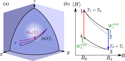
Figure 1: (a) The evolution of the quantum state on Bloch sphere during the adiabatic process. We take the Bloch sphere for the two-level system as an example. The purple-solid (black-dashed) line presents the finite-time evolution (the adiabatic trajectory). (b) The energy-control ($\left\langle H\right\rangle-R$) diagram for the quantum Otto cycle. The solid (dashed) line shows the finite-time (quasi-static) Otto cycle. To allow the fair comparison, we set the highest (lowest) temperature $T_{1}$ ($T_{3}$) equal to that of hot (cold) bath $T_{h}$ ($T_{c}$).

At the beginning of adiabatic process, the system is initially prepared at a thermal equilibrium state

$$\rho(0)=\frac{e^{-\beta H[\vec{R}(0)]}}{\mathrm{Tr}e^{-\beta H[\vec{R}(0)]}},$$ (1)

with inverse temperature $\beta$. $H[\vec{R}(t)]$ is the Hamiltonian with the control parameter $\vec{R}(t)$. The macroscopic parameters are tuned from $\vec{R}\left(0\right)$ at the beginning to $\vec{R}\left(\tau\right)$ at the end. The evolution of the system during $0<t<\tau$ is controlled by a time-dependent Hamiltonian $H(t)=H[\vec{R}(t)]$ as

$$\dot{\rho}=-i[H(t),\rho].$$ (2)

Under the instantaneous basis $\left\{\left|n(t)\right\rangle\right\}$, the time-dependent Hamiltonian is diagonal

$$H(t)=\sum_{n}E_{n}(t)\left|n(t)\right\rangle\left\langle n(t)\right|,$$ (3)

and the initial state is rewritten as $\rho(0)=\sum_{n}p_{n}\left|n(0)\right\rangle\left\langle n(0)\right|$ with the thermal distribution

$$p_{n}=\frac{e^{-\beta E_{n}(0)}}{\sum_{m}e^{-\beta E_{m}(0)}}.$$ (4)

In the adiabatic process, the density matrix at any time in interval $[0,\tau]$ is

$$\rho(t)=\sum_{n}p_{n}\left|\psi_{n}(t)\right\rangle\left\langle\psi_{n}(t)\right|,$$ (5)

where $\left|\psi_{n}(t)\right\rangle$ follows the Schroedinger equation

$$i\frac{\partial}{\partial t}\left|\psi_{n}(t)\right\rangle=H(t)\left|\psi_{n}(t)\right\rangle,$$ (6)

with the initial state $\left|\psi_{n}(0)\right\rangle=\left|n(0)\right\rangle$. The evolution of the instantaneous state $\left|n(t)\right\rangle$ and the state $\left|\psi_{n}(t)\right\rangle$ is illustrated in Fig. 1(a). The purple-solid lines show the trajectories for finite-time adiabatic processes with changing control time $\tau$, and the black-dashed line presents the evolution of the instantaneous basis. With the increasing control time $\tau$, the state $\left|\psi_{n}(t)\right\rangle$ approaches to the adiabatic trajectory $\left|n(t)\right\rangle$.

The finite-time effect is reflected through the work extraction during the adiabatic process. Since the system is isolated from any baths in the adiabatic processes, no heat is generated during the whole process. The work done equals to the change of the internal energy $W(\tau)=\mathrm{Tr}[\rho(\tau)H(\tau)-\rho(0)H(0)]$, explicitly as

$$W(\tau)=\sum_{n}p_{n}[\langle\psi_{n}\left(\tau\right)|H\left(\tau\right)|\psi_{n}\left(\tau\right)\rangle-E_{n}\left(0\right)].$$ (7)

To show the difference between the finite-time adiabatic process and its quasi-static counterpart, we define the extra work as

$$W^{(\mathrm{ex})}(\tau)=W(\tau)-W_{\mathrm{adi}},$$ (8)

where $W_{\mathrm{adi}}=\sum_{n}p_{n}[E_{n}(\tau)-E_{n}(0)]$ is the work done during the quasi-static adiabatic process. One property of the extra work for the finite-time adiabatic process is its non-negativity $W^{(\mathrm{ex})}(\tau)\geq 0$, which is proved with details in Appendix A. The non-negativity of the extra work ensures a lower efficiency of the finite-time Otto cycle than that of the quasi-static one. Such non-negativity was previously known as the minimal work principle: For an initial thermal state, the quasi-static adiabatic process generates the minimal work when the energy level does not cross (Allahverdyan and Nieuwenhuizen, 2005).

The key is to obtain the extra work via the dynamics of wave-function $\left|\psi_{n}(t)\right\rangle$, which is expanded in the instantaneous basis $\{|l(t)\rangle\}$ as

$$\left|\psi_{n}(t)\right\rangle=\sum_{l}c_{nl}(t)e^{-i\phi_{l}\left(t\right)}\left|l(t)\right\rangle,$$ (9)

where $\phi_{l}\left(t\right)=\int_{0}^{t}E_{l}(t^{\prime})dt^{\prime}$ is the dynamical phase. The amplitude $c_{nl}(t)$ is obtained by using the adiabatic perturbation theory (Sun, 1988; Rigolin et al., 2008), where $\nu=1/\tau$ is treated as the perturbation parameter for long operation time. Based on the high-order adiabatic approximation (Sun, 1988), we obtain $c_{nl}(\tau)$ to the first order in Appendix B as

$$c_{nl}^{[1]}(\tau)=\begin{cases}e^{i\tau\tilde{\gamma}_{n}\left(1\right)}&n=l\\ -i\nu[\tilde{T}_{nl}\left(1\right)e^{-i\tau(\tilde{\phi}_{n}\left(1\right)-\tilde{\phi}_{l}\left(1\right))+i\tilde{\gamma}_{n}\left(1\right)}-\tilde{T}_{nl}\left(0\right)e^{i\tilde{\gamma}_{l}\left(1\right)}]&n\neq l\end{cases},$$ (10)

where the function with tilde is rewritten with the rescaled time parameter $s=t/\tau$. Here, the Berry phase is given by

$$\tilde{\gamma}_{l}\left(s\right)=i\int_{0}^{s}\tilde{\Gamma}_{ll}(s^{\prime})ds^{\prime},$$ (11)

with the notation $\tilde{\Gamma}_{lm}(s)=\left\langle\tilde{l}(s)\right|d/ds\left|\tilde{m}(s)\right\rangle$; The non-adiabatic transition rate is

$$\tilde{T}_{nl}\left(s\right)=\frac{\tilde{\Gamma}_{ln}(s)}{\tilde{E}_{n}(s)-\tilde{E}_{l}(s)},$$ (12)

presenting the transition from the state $\left|\tilde{n}(s)\right\rangle$ with the eigen-energy $\tilde{E}_{n}\left(s\right)$ to another state $|\tilde{l}(s)\rangle$. For the quasi-static adiabatic process $\nu\rightarrow 0$, the first order term vanishes and the state $\left|\psi_{n}(t)\right\rangle$ remains on the instantaneous eigen-state $\left|n(t)\right\rangle$ with a time-dependent phase. In turn, our definition of the extra work is appropriate in the sense of retaining quantum adiabatic limit (Quan et al., 2007). Here, we clarify the distinction and connection between quantum adiabacity and thermodynamic adiabacity. Quantum adiabacity means that population of the energy eigen-states remains unchanged during the whole process, while thermodynamic adiabacity indicates no heat exchange between the system and the environment. In the finite-time adiabatic processes, the unitary evolution of an isolated quantum system ensures the thermodynamic adiabacity, but quantum adiabacity is not usually satisfied due to the non-adiabatic transition between different eigen-states. The rigorous quantum adiabaticity only holds at the infinite control time limit $\nu\rightarrow 0$. The quantum non-adiabaticity is responsible for the extra work needed to complete the adiabatic process in finite time.

With the amplitude $c_{nl}(\tau)$, the extra work by Eq. (8) is simplified as

$$W^{\mathrm{(ex)}}(\tau)=\sum_{n,l\neq n}p_{n}[\tilde{E}_{l}(1)-\tilde{E}_{n}(1)]|c_{nl}(\tau)|^{2}.$$ (13)

From the first-order adiabatic approximation result by Eq. (10), the value of the absolute square $\left|c_{nl}^{[1]}(\tau)\right|^{2},\,n\neq l$ is divided into the mean part and the oscillating part as

$$\left|c_{nl}^{[1]}(\tau)\right|^{2}=\left(\left|c_{nl}^{[1]}(\tau)\right|^{2}\right)^{\mathrm{(mean)}}+\left(\left|c_{nl}^{[1]}(\tau)\right|^{2}\right)^{\mathrm{(osc)}},$$ (14)

where the mean part is

$$\left(\left|c_{nl}^{[1]}(\tau)\right|^{2}\right)^{\mathrm{(mean)}}=\frac{1}{\tau^{2}}\left(\left|\tilde{T}_{nl}\left(1\right)\right|^{2}+\left|\tilde{T}_{nl}\left(0\right)\right|^{2}\right),$$ (15)

and the oscillating part is

$$\left(\left|c_{nl}^{[1]}(\tau)\right|^{2}\right)^{\mathrm{(osc)}}=-\frac{2}{\tau^{2}}\mathrm{Re}\left[e^{-i\tau[\tilde{\phi}_{n}(1)-\tilde{\phi}_{l}(1)]+i[\tilde{\gamma}_{n}(1)-\tilde{\gamma}_{l}(1)]}\tilde{T}_{nl}\left(1\right)\tilde{T}_{nl}^{*}\left(0\right)\right].$$ (16)

To the first order, $|c_{nl}^{[1]}(\tau)|^{2}$ is proportional to $\nu^{2}$, leading to the $\mathcal{C}/\tau^{2}$ scaling of the extra work. This scaling is different from the $1/\tau$ scaling of the irreversible entropy production in the finite-time isothermal process of the Carnot-like cycle (Shiraishi et al., 2016; Ma et al., 2018). Corresponding to Eqs. (15) and (16), the extra work $W^{(\mathrm{ex})}(\tau)=W^{(\mathrm{mean})}(\tau)+W^{(\mathrm{osc})}(\tau)$ by Eq. (13) is divided into the mean extra work

$$W^{(\mathrm{mean})}(\tau) =\frac{\Sigma}{\tau^{2}},$$ (17)

and the oscillating extra work

$$W^{(\mathrm{osc})}(\tau) =\frac{\omega\left(\tau\right)}{\tau^{2}}.$$ (18)

The mean extra work decreases decreases monotonously with the increasing control time $\tau$, while the oscillating extra work oscillates around $0$, and contributes the fluctuation in the extra work. The coefficients in Eqs. (17) and (18) follow explicitly as

$$\Sigma=\sum_{n,l\neq n}p_{n}[\tilde{E}_{l}(1)-\tilde{E}_{n}(1)][|\tilde{T}_{nl}\left(1\right)|^{2}+|\tilde{T}_{nl}\left(0\right)|^{2}],$$ (19)

and

$$\omega(\tau)=-\sum_{n,l\neq n}2p_{n}[\tilde{E}_{l}(1)-\tilde{E}_{n}(1)]\mathrm{Re}\{\tilde{T}_{nl}\left(1\right)\tilde{T}_{nl}^{*}\left(0\right)e^{-i\tau(\tilde{\phi}_{n}\left(1\right)-\tilde{\phi}_{l}\left(1\right))+i(\tilde{\gamma}_{n}\left(1\right)-\tilde{\gamma}_{l}\left(1\right))}\}.$$ (20)

The impact of the control scheme is reflected through the transition amplitude $\tilde{T}_{nl}\left(s\right)$. Interestingly, the mean extra work, to the leading order, only depends on the initial (final) transition amplitude $\tilde{T}_{nl}\left(0\right)$ ($\tilde{T}_{nl}\left(1\right)$), instead of the whole trajectory. And the oscillating one relies on the trajectory only through the dynamical phase $\tilde{\phi}_{n}\left(s\right)$ and the Berry phase $\tilde{\gamma}_{n}\left(s\right)$.

For the oscillating extra work, $\omega(\tau)$ oscillates around $0$ with the increasing control time $\tau$. When we consider the system with the incommensurable energy difference $\tilde{E}_{l}(s)-\tilde{E}_{n}(s)$ for different sets of indexes $l$ and $n$, the oscillation of $\omega(\tau)$ contains different frequency $\tilde{\phi}_{n}\left(1\right)-\tilde{\phi}_{l}\left(1\right)$. In the summation of $\omega\left(\tau\right)$, the terms with different phase $\tilde{\phi}_{n}\left(1\right)-\tilde{\phi}_{l}\left(1\right)$ cancel out each other. In the follow discussion, we will neglect the oscillating term in Eq. (18). Yet, this oscillating terms may introduce higher efficiency for system with few energy levels, e.g. the two-level system (Erdman et al., 2018).

III Efficiency at maximum power for quantum Otto heat engine

With the $\mathcal{C}/\tau^{2}$ scaling of the extra work, we evaluate the performance of quantum Otto engine by the efficiency and the output power. The Otto cycle is illustrated via the $\left\langle H\right\rangle-\vec{R}$ diagram in Fig. 1(b). The solid line shows the finite-time Otto cycle, while the dashed line shows the corresponding quasi-static one. The work done during the two adiabatic processes ($1\rightarrow 2$) and ($3\rightarrow 4$) are $W_{1}\left(\tau_{1}\right)<0$ and $W_{3}(\tau_{3})>0$ with the change of external parameters ($R_{0}\leftrightarrow R_{1}$) respectively. The heat engine contacts with the hot (cold) bath and reaches the equilibrium with the temperature $T_{1}$ ($T_{3}$) in the isochoric heating ($4\rightarrow 1$) (isochoric cooling $(2\rightarrow 3)$) with the fixed parameter $R_{0}$ ($R_{1}$).

The performance of quantum Otto engine is evaluated by the efficiency and the output power. We need the net work and the heat exchange under the adiabatic perturbation approximation. For the two adiabatic processes, the work is

$$W_{i}\left(\tau_{i}\right) \equiv\mathrm{Tr}[\rho_{i+1}H_{i+1}]-\mathrm{Tr}[\rho_{i}H_{i}]$$ (21)

$$=W_{i}^{\mathrm{adi}}+\frac{\Sigma_{i}}{\tau_{i}^{2}},\>i=1,3,$$ (22)

where $\tau_{i}$ is the corresponding control time, and $\Sigma_{i}$ is the corresponding coefficients related to the control scheme. The work in the quasi-static adiabatic process is given by

$$W_{i}^{\mathrm{adi}}=\mathrm{Tr}[\rho_{i+1}^{\mathrm{adi}}H_{i+1}]-\mathrm{Tr}[\rho_{i}H_{i}].$$ (23)

We consider the relaxation time in the isochoric processes is much shorter than the control time $\tau_{i},\,i=1,3$ in the adiabatic processes. The time consuming of the isochoric processes is neglected, and the system is fully thermalized after the isochoric processes. The heat exchange with the hot bath during the isochoric process is

$$Q_{h} \equiv\mathrm{Tr}[\rho_{4}H_{4}]-\mathrm{Tr}[\rho_{1}H_{1}]$$ (24)

$$=Q_{h}^{\mathrm{adi}}-\frac{\Sigma_{3}}{\tau_{3}^{2}}.$$ (25)

The net work for the whole cycle is

$$W_{\mathrm{T}}=-[W_{1}\left(\tau_{1}\right)+W_{3}\left(\tau_{3}\right)],$$ (26)

and the efficiency is

$$\eta=\frac{W_{\mathrm{T}}}{Q_{h}}.$$ (27)

Combing the equations for $W_{i}(\tau_{i})$ and $W_{i}^{\mathrm{adi}}$, the power $P=W_{\mathrm{T}}/(\tau_{1}+\tau_{3})$ for the finite-time Otto heat engine follows explicitly

$$P =\frac{W_{\mathrm{T}}^{\mathrm{adi}}}{\tau_{1}+\tau_{3}}-\frac{1}{\tau_{1}+\tau_{3}}\left(\frac{\Sigma_{1}}{\tau_{1}^{2}}+\frac{\Sigma_{3}}{\tau_{3}^{2}}\right),$$ (28)

with the efficiency

$$\eta =\frac{W_{\mathrm{T}}^{\mathrm{adi}}-\left(\Sigma_{1}/\tau_{1}^{2}+\Sigma_{3}/\tau_{3}^{2}\right)}{W_{\mathrm{T}}^{\mathrm{adi}}/\eta^{\mathrm{adi}}-\Sigma_{3}/\tau_{3}^{2}}.$$ (29)

Here, $W_{\mathrm{T}}^{\mathrm{adi}}=-(W_{1}^{\mathrm{adi}}+W_{3}^{\mathrm{adi}})$ is the net work for the quasi-static Otto cycle with the corresponding efficiency $\eta^{\mathrm{adi}}=W_{\mathrm{T}}^{\mathrm{adi}}/Q_{h}^{\mathrm{adi}}$.

According to the optimal condition of the maximum power $\partial P/\partial\tau_{1}=0,\,\partial P/\partial\tau_{3}=0$, the current finite-time Otto engine reaches its maximum power

$$P_{\mathrm{max}}=2\left[\frac{W_{\mathrm{T}}^{\mathrm{adi}}}{3\left(\Sigma_{1}^{1/3}+\Sigma_{3}^{1/3}\right)}\right]^{\frac{3}{2}}$$ (30)

at the optimal operation time $\tau_{1}^{*}=[3(\Sigma_{1}^{2/3}\Sigma_{3}^{1/3}+\Sigma_{1})/W_{\mathrm{T}}^{\mathrm{adi}}]^{1/2}$ and $\tau_{3}^{*}=[3(\Sigma_{3}^{2/3}\Sigma_{1}^{1/3}+\Sigma_{3})/W_{\mathrm{T}}^{\mathrm{adi}}]^{1/2}$. The corresponding efficiency at the maximum power (EMP) is

$$\eta_{\mathrm{EMP}} =\frac{2\eta^{\mathrm{adi}}}{3-\frac{\eta^{\mathrm{adi}}}{1+(\Sigma_{1}/\Sigma_{3})^{1/3}}},$$ (31)

which depends on the ratio $\Sigma_{1}/\Sigma_{3}$, and the efficiency $\eta^{\mathrm{adi}}$ of the quasi-static Otto cycle. In the limit $\Sigma_{1}/\Sigma_{3}\rightarrow 0$, the EMP reaches the upper bound

$$\eta_{\mathrm{EMP}}^{+}=\frac{2\eta^{\mathrm{adi}}}{3-\eta^{\mathrm{adi}}}.$$ (32)

In the limit $\Sigma_{1}/\Sigma_{3}\rightarrow\infty$, the EMP reaches the lower bound

$$\eta_{\mathrm{EMP}}^{-}=\frac{2}{3}\eta^{\mathrm{adi}}.$$ (33)

We obtain the main result in Eq. (31) with the first-order quantum adiabatic approximation, where the inverse control time $\nu$ is the perturbation parameter. The result relies on two key factors, i.e, the long control time (Sun, 1988; Rigolin et al., 2008) $\tau$ and the non-level crossing condition (Allahverdyan and Nieuwenhuizen, 2005). To obtain the EMP, we have neglected the oscillating extra work with the observation of incommensurability of the typical energy levels. Yet, such oscillating part can introduce interesting effects on EMP for small quantum systems, e.g., the minimal quantum heat engine with two-level system (Linden et al., 2010).

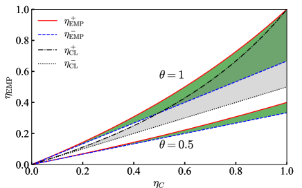
Figure 2: Comparison between the EMP of finite-time quantum Otto cycle and Carnot-like cycle. The red-solid (blue-dashed) lines show the upper (lower) for the EMP of finite-time Otto cycle with two sets of $\theta$. The black-dashdotted (black-dotted) line presents the upper (lower) bound $\eta_{\mathrm{CL}}^{+}$ ( $\eta_{\mathrm{CL}}^{-}$) for the EMP of Carnot-like cycle.

We turn to compare the EMP of the finite-time Otto cycle with that of the Carnot-like cycle. For the Carnot-like cycle, the upper bound (Esposito et al., 2010; Ma et al., 2018) is $\eta_{\mathrm{CL}}^{+}=\eta_{\mathrm{C}}/(2-\eta_{\mathrm{C}})$, where $\eta_{\mathrm{C}}=1-T_{c}/T_{h}$ is the Carnot efficiency for heat engine working between the low temperature $T_{c}$ and the high temperature $T_{h}$ baths. To allow a fair comparison, we set the highest (lowest) temperature $T_{1}$ ($T_{3}$) in the isochoric process to be the temperature for the hot (cold) bath, namely $T_{1}=T_{h}$ ($T_{3}=T_{c}$). To surpass the EMP of Carnot-like heat engine ($\eta_{\mathrm{EMP}}^{+}>\eta_{\mathrm{CL}}^{+}$), it is required that

$$\eta^{\mathrm{adi}}>\frac{3\eta_{\mathrm{C}}}{4-\eta_{\mathrm{C}}}.$$ (34)

The efficiency $\eta^{\mathrm{adi}}$ of the quasi-static Otto is always smaller than the Carnot efficiency $\eta_{\mathrm{C}}$, namely, $\eta^{\mathrm{adi}}<\eta_{\mathrm{C}}$.

In Fig. 2, we show the EMP of both the Carnot-like cycle and the current quantum Otto cycle. We set the efficiency of the corresponding quasi-static Otto heat engine as $\eta^{\mathrm{adi}}=\theta\eta_{\mathrm{C}}$ with the ratio $\theta\in[0,1]$. For the finite-time quantum Otto cycle, the upper (lower) bound $\eta_{\mathrm{EMP}}^{+}$ ($\eta_{\mathrm{EMP}}^{-}$) is plotted as the red-solid (blue-dashed) line. Two sets of the ratios $\theta=0.5$ and $\theta=1$ are plotted. For the Carnot-like heat engine, the black-dashdotted and the black-dotted lines give the upper bound $\eta_{\mathrm{CL}}^{+}$ and the lower bound $\eta_{\mathrm{CL}}^{-}=\eta_{C}/2$ respectively (Esposito et al., 2010). For $\theta=1$, the curve shows that the EMP of the finite-time quantum Otto cycle exceeds the one for the finite-time Carnot cycle. Such higher EMP is achievable only at the region $\theta>3/4$. The curves for $\theta=0.5$ show the lower efficiency than that of the Carnot-like cycle. The current generic model implies the possibility to surpass the EMP of the Carnot-like cycle by choosing the proper efficiency of the quasi-static Otto cycle $\eta^{\mathrm{adi}}$ larger than $3\eta_{C}/4$. We will realize such Otto cycle with an example of the quantum piston model.

IV Finite-time quantum Otto engine on piston model

We illustrate the $\mathcal{C}/\tau^{2}$ scaling of extra work during the adiabatic process with the widely used quantum piston model (Makowski and Dembiński, 1991; Doescher and Rice, 1969; Quan and Jarzynski, 2012) and show the surpassed EMP of Carnot-like engines with the designed finite-time Otto cycle. Now we consider a concrete model of a single particle trapped in a square box with the Hamiltonian,

$$H(t) =-\frac{1}{2M}\frac{\partial^{2}}{\partial x^{2}}+V(x,t).$$ (35)

where $M$ is the mass of the particle, and $V(x,t)$ is the square potential

$$V(x,t)=\begin{cases}\infty&x<0,\,x>L(t)\\ 0&0\leq x\leq L(t)\end{cases}.$$ (36)

The controllable length $L(t)$ serves as the tuning parameter $R\left(t\right)$ as discussed in the generic model. The advantage of the current model is the existence of an exact solution for the linear control protocol (Makowski and Dembiński, 1991; Doescher and Rice, 1969)

$$L(t)=L_{0}+(L_{1}-L_{0})\frac{t}{\tau},$$ (37)

which allows a direct validation of the scaling in Eq. (17) derived by the adiabatic perturbation theory. Here, $L_{0}$ ($L_{1}$) is the initial (final) length of the box during the adiabatic process.

For this control scheme $\tilde{L}\left(s\right)=L\left(s\tau\right)$, the instantaneous wave-function is

$$\left\langle x\right.\left|\tilde{n}\left(s\right)\right\rangle=\sqrt{\frac{2}{\tilde{L}}}\sin\left(\frac{n\pi}{\tilde{L}}x\right),$$ (38)

with the corresponding energy

$$\tilde{E}_{n}\left(s\right)=\frac{\pi^{2}n^{2}}{2M\tilde{L}^{2}}.$$ (39)

The non-adiabatic transition rate is

$$\tilde{T}_{nl}(s) =-\frac{4Mnl(-1)^{l+n}(L_{1}-L_{0})}{\pi^{2}(n^{2}-l^{2})^{2}}\tilde{L}(s).$$ (40)

Under long control time limit, we obtain the asymptotic result of the extra work as

$$W^{\mathrm{(mean)}}(\tau) =\frac{ML_{1}^{2}(1-r)^{2}(1+r^{2})}{\tau^{2}}(\frac{1}{6}-\sum_{n=1}^{\infty}\frac{p_{n}}{4\pi^{2}n^{2}}),$$ (41)

with the expansion ratio $r=L_{0}/L_{1}$. The initial thermal distribution is

$$p_{n}(\beta,L_{0})=\frac{e^{-\frac{\beta\pi^{2}n^{2}}{2L_{0}^{2}M}}}{Z(\beta,L_{0})},$$ (42)

with the initial inverse temperature $\beta=1/k_{B}T$. The partition function is

$$Z(\beta,L)=\frac{1}{2}\vartheta_{3}\left(0,e^{-\frac{\beta\pi^{2}}{2L^{2}M}}\right)-\frac{1}{2},$$ (43)

where $\vartheta_{3}\left(0,q\right)=2\sum_{n=1}^{\infty}q^{n^{2}}+1$ is the Elliptic-Theta function. The detailed derivation of Eq. (41) is given in Appendix C, where the oscillating extra work is also obtained analytically. At high temperature limit $\beta\rightarrow 0$, the thermal de Broglie wavelength $\lambda_{\mathrm{th}}=(2\pi\beta/M)^{1/2}$ is much smaller than the length of the box and the summation $\sum_{n=1}^{\infty}p_{n}/(4\pi^{2}n^{2})$ in Eq. (41) can be neglected. Thus, we obtain the approximation for the mean extra work in Eq. (41) as

$$W^{(\mathrm{mean})}(\tau)\approx\frac{ML_{1}^{2}(1-r)^{2}(1+r^{2})}{6\tau^{2}}.$$ (44)

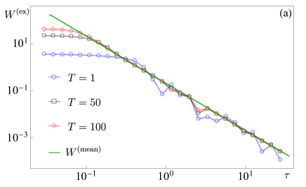
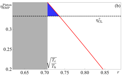
Figure 3: (a) The $\mathcal{C}/\tau^{2}$ scaling for the extra work in the finite-time adiabatic expansion process on quantum piston model, with the length chosen as $L_{0}=1$ and $L_{1}=2$. The blue circle, black square, and red diamaond show the exact numerical result with the initial temperatures $T=1,\,50,\,100$, respectively. The green-solid line presents the analytical result of the mean extra work for large $\tau$ in Eq. (17). (b) The EMP of the finite-time quantum Otto cycle as the function of the expansion ratio $r=L_{0}/L_{1}$ (the red-solid line), with the fixed temperature ratio $T_{c}/T_{h}=1/2$. The black-dashed horizontal line presents the upper bound of the Carnot-like cycle $\eta_{\mathrm{CL}}^{+}$. The gray area shows the engine with negative output power $P<0$, and the blue area shows the higher EMP than that of the Carnot-like cycle.

By controlling the length of the trap, we realize the finite-time quantum Otto cycle with the current quantum piston model. The two lengths for the adiabatic process are $L_{0}$ and $L_{1}$ with $L_{0}<L_{1}$. For the quasi-static Otto cycle, the efficiency of the engine is $\eta^{\mathrm{adi}}=1-r^{2}$ and the net work of the whole cycle has a simple result at high temperature

$$W^{\mathrm{adi}}=\frac{k_{B}}{2}\left(T_{h}r^{2}-T_{c}\right)(\frac{1}{r^{2}}-1).$$ (45)

For the finite-time adiabatic process, the coefficients of the mean extra work with linear control schemes are

$$\Sigma_{1}=\frac{M(1-r)^{2}\left(1+r^{2}\right)L_{1}^{2}}{6},$$ (46)

and

$$\Sigma_{3}=\frac{M(1-r)^{2}\left(1+r^{2}\right)L_{1}^{2}}{6r^{2}}.$$ (47)

Fig. 3(a) validates the $\mathcal{C}/\tau^{2}$ scaling of the extra work $W^{(\mathrm{mean})}(\tau)$ in Eq. (44) during the expansion of the quantum piston model. We set the mass $M=1$ and the Boltzmann constant as $k_{B}=1$ in all the later calculation. During the expansion, the length of the box varies from the initial value $L_{0}=1$ to the final value $L_{1}=2$. Exact results are obtained with analytical solution of the time-dependent Schroedinger equation in Ref. (Doescher and Rice, 1969; Makowski and Dembiński, 1991; Quan and Jarzynski, 2012). We choose the initial thermal states with different temperatures $T=1,$ $50$ and $100$, marked with blue circle, black square, and red diamond respectively. The oscillation of the extra work becomes weaker for higher temperature. For long control time, the exact numerical result of the extra work (the markers) matches with the analytical one (the green-solid line), demonstrating the $\mathcal{C}/\tau^{2}$ scaling of the extra work.

The maximum power for the piston model is obtained as

$$P_{\mathrm{max}}^{\mathrm{Piston}} =\frac{1}{3L_{1}}\left(\frac{k_{B}(T_{h}r^{2}-T_{c})(1-r^{2})}{[M(1-r)^{2}\left(1+r^{2}\right)]^{\frac{1}{3}}(r^{2}+r^{\frac{4}{3}})}\right)^{\frac{3}{2}},$$ (48)

by choosing the optimal control time $\tau_{1}^{*}$ and $\tau_{3}^{*}$. And the corresponding efficiency is obtained by Eq. (31)

$$\eta_{\mathrm{EMP}}^{\mathrm{Piston}}=\frac{2\eta^{\mathrm{adi}}}{3-\frac{\eta^{\mathrm{adi}}}{(1-\eta^{\mathrm{adi}})^{1/3}+1}}.$$ (49)

The detailed derivation of Eqs. (48) and (49) together with the optimal control time $\tau_{1}^{*}$ and $\tau_{3}^{*}$ is given in Appendix C.

In Fig. 3(b), we plot the EMP $\eta_{\mathrm{EMP}}^{\mathrm{Piston}}$ in Eq. (49) as the function of the expansion ratio $r$. The requirement of the positive power in Eq. (48) implies the constraint for the expansion ratio $r$ as $\sqrt{T_{c}/T_{h}}<r<1$, shown as the white area. The upper bound $\eta_{\mathrm{CL}}^{+}$ of the Carnot-like cycle is plotted as the horizontal black-dashed line, with the fixed temperature ratio $T_{c}/T_{h}=1/2$. The EMP $\eta_{\mathrm{EMP}}^{\mathrm{Piston}}$ of the current piston model is shown as the red solid line. Fig. 3(b) indicates the higher EMP of the finite-time quantum Otto cycle than that of the Carnot-like cycle at the region $1/\sqrt{2}<r<0.736$, illustrated as the blue area. The number $0.736$ is obtained by solving the equation $\eta_{\mathrm{EMP}}^{\mathrm{Piston}}=\eta_{\mathrm{CL}}^{+}$. In the current model, the piston is controlled with the simplest scheme that the expansion ratio is the only optimizing parameter for the EMP $\eta_{\mathrm{EMP}}^{\mathrm{Piston}}$. More complicated control scheme (Makowski and Dembiński, 1991) can be considered to show more flexible tuning EMP beyond the Carnot-like cycle.

V Conclusion & Remarks

In this paper, we have studied the finite-time effect of adiabatic processes. With the high-order adiabatic approximation, we have proved the universal $\mathcal{C}/\tau^{2}$ scaling for the extra work in the finite-time adiabatic processes, and validated it with the quantum piston model. It is meaningful to test this universal scaling on other complex quantum systems from both theoretical and experimental aspects. The current experimental setup on the trapped Fermi gas (Deng et al., 2016, 2018) can be directly applied to verify the $\mathcal{C}/\tau^{2}$ scaling of the extra work. One needs to choose a fixed protocol of the adiabatic process, and measures the work to complete the adiabatic process for different control time $\tau$.

Moreover, we described a new class of finite-time quantum heat engine with Otto cycle. Importantly, we showed such cycle is capable to achieve higher efficiency at maximum power than that of the widely-used Carnot-like cycle. The better performance of the quantum Otto cycle will attract attentions for new designs of the quantum heat engine, instead of focusing on optimizing the Carnot-like cycle in finite time. It is proposed that the quantum Otto cycle can be implemented on a single-ion engine (Abah et al., 2012; Roßnagel et al., 2014). Our study contributes to the further optimization of the concrete finite-time quantum engine in the experiments.

In the derivation of the $\mathcal{C}/\tau^{2}$ scaling for the extra work, the oscillating extra work is neglected due to the incommensurable energy difference of the complex system. Yet, for the quantum heat engine with work matter consisting of few energy levels, the oscillating extra work can affect the performance of the quantum Otto engine. The oscillating behavior of the extra work leads to a quantum Otto engine with high efficiency (Peterson et al., ; de Assis et al., 2019), and will induce new effect on the efficiency-power constraint relation (Chen et al., ).

Appendix A Positivity of the Extra Work

In this appendix, we prove the positivity of the extra work by using the Schur-Horn theorem. We remark that the proof of the positive extra work was already presented elsewhere (Allahverdyan and Nieuwenhuizen, 2005). However, our version of the proof with the Schur-Horn theorem is new and straightforward. Generally, we assume the energy levels shift remaining the order $\tilde{E}_{1}(s)<\tilde{E}_{2}(s)...<\tilde{E}_{n}(s)<...$ during the whole adiabatic process (Allahverdyan and Nieuwenhuizen, 2005). For an initial thermal state, the extra work from Eq. (60) is explicitly written as

$$W^{\mathrm{(ex)}}(\tau)=\sum_{l=1}^{\infty}\lambda_{ll}\tilde{E}_{l}(1)-\sum_{n=1}^{\infty}p_{n}\tilde{E}_{n}(1),$$ (50)

with the notation $\lambda_{ll}=\sum_{n=1}^{\infty}p_{n}\left|c_{nl}(\tau)\right|^{2}$. We rearrange the summation and obtain

$$W^{\mathrm{(ex)}}(\tau)=\tilde{E}_{1}(1)\left[\sum_{l=1}^{\infty}\left(\lambda_{ll}-p_{l}\right)\right]+\sum_{j=2}^{\infty}\left(\tilde{E}_{j}(1)-\tilde{E}_{j-1}(1)\right)\left[\sum_{l=j}^{\infty}\left(\lambda_{ll}-p_{l}\right)\right].$$ (51)

The first term on the right hand of Eq. (51) is zero due to the normalized condition for the probability $\sum_{l=1}^{\infty}\lambda_{ll}=\sum_{l=1}^{\infty}p_{l}=1$. We prove the second term on the right hand side is non-negative based on Schur-Horn theorem (Horn, 1954). Since $\tilde{E}_{j}(1)-\tilde{E}_{j-1}(1)>0$, we only need to prove $\sum_{l=j}^{\infty}\lambda_{ll}\geq\sum_{l=j}^{\infty}p_{l}$.

Here, $\lambda_{ll}$ can be regarded as the diagonal element for the Hermite matrix $\lambda_{lm}=\sum_{n=1}^{\infty}p_{n}\left[c_{nl}(\tau)\right]^{*}c_{nm}(\tau)$, which is obtained from the diagonal matrix with the diagonal element $p_{n}$ through the unitary transform $c_{nm}(\tau)$. Thus, the eigenvalue of this Hermitian matrix is exact $p_{n}$. We re-sequence the diagonal terms $\lambda_{ll}$ in the non-increasing order as $\tilde{\lambda}_{11}\geq\tilde{\lambda}_{22}\geq...\geq\tilde{\lambda}_{nn}...$. Schur-Horn theorem (Horn, 1954) presents the following inequality

$$\sum_{l=1}^{j-1}\tilde{\lambda}_{ll}\leq\sum_{l=1}^{j-1}p_{l},\,j\geq 2$$ (52)

for a Hermitian matrix with the diagonal terms $\tilde{\lambda}_{ll}$ and eigenvalue $p_{l}$ both in non-increasing order. Together with the normalization of the probability, we have the inequality $\sum_{l=j}^{\infty}\tilde{\lambda}_{ll}\geq\sum_{l=j}^{\infty}p_{l},\,j\geq 1$. Since $\tilde{\lambda}_{ll}$ gives the non-increasing order for $\lambda_{ll}$, we have apparently $\sum_{l=j}^{\infty}\lambda_{ll}\geq\sum_{l=j}^{\infty}\tilde{\lambda}_{ll}$, and thus $\sum_{l=j}^{\infty}\left(\lambda_{ll}-p_{l}\right)\geq 0$.

Therefore, we have proven $W^{\mathrm{(ex)}}(\tau)\geq 0$: the extra work for an initial thermal state is non-negative when the energy level does not cross during the finite-time adiabatic process.

Appendix B First-order Adiabatic Approximation and the Extra Work

This appendix is devoted to showing the detailed derivation of the non-adiabatic correction for the extra work for finite-time adiabatic processes based on higher-order adiabatic approximation (Sun, 1988). The Schroedinger equation $i\partial_{t}\left|\psi_{n}(t)\right\rangle=H(t)\left|\psi_{n}(t)\right\rangle$ results in the following differential equation for the amplitude $c_{nl}(t)$

$$\frac{d}{dt}c_{nl}(t)+c_{nl}(t)\Gamma_{ll}(t)+\sum_{m\neq l}c_{nm}(t)e^{-i\left(\phi_{m}(t)-\phi_{l}(t)\right)}\Gamma_{lm}(t)=0,$$ (53)

with the dynamical phase $\phi_{l}(t)=\int_{0}^{t}E_{l}(t^{\prime})dt^{\prime}$ and the notation $\Gamma_{lm}(t)=\left\langle l(t)\right|d/dt\left|m(t)\right\rangle$. We consider for a given protocol of the adiabatic process $\tilde{H}(s)=H(\tau s)=\sum_{n}\tilde{E}_{n}(s)\left|\tilde{n}(s)\right\rangle\left\langle\tilde{n}(s)\right|$ with $\tau$ as the control time, where $\left|\tilde{n}(s)\right\rangle=\left|n(\tau s)\right\rangle$, $\tilde{E}_{n}(s)=E_{n}(\tau s)$. Representing the amplitude $b_{nl}(s)=c_{nl}(\tau s)$ with the rescaled time parameter $s$, the differential equation is rewritten for $b_{nl}(s)$ as

$$\frac{d}{ds}b_{nl}(s)+b_{nl}(s)\tilde{\Gamma}_{ll}(s)+\sum_{m\neq l}b_{nm}(s)e^{-i\tau\left(\tilde{\phi}_{m}(s)-\tilde{\phi}_{l}(s)\right)}\tilde{\Gamma}_{lm}(s)=0,$$ (54)

where the notation$\tilde{\Gamma}_{lm}(s)=\left\langle\tilde{l}(s)\right|\frac{d}{ds}\left|\tilde{m}(s)\right\rangle$ and the dynamical phase $\tilde{\phi}_{l}(s)=\int_{0}^{s}\tilde{E}_{l}(s^{\prime})ds^{\prime}$ are given by the rescaled time parameter $s$.

Based on the high-order adiabatic approximation in Ref. (Sun, 1988), we obtain the solution of $b_{nl}^{[1]}(s)=b_{nl}^{(0)}(s)+b_{nl}^{(1)}(s)/\tau$ to the first order of $1/\tau$, where $b_{nl}^{(0)}(s)$ and $b_{nl}^{(1)}(s)$ satisfy the following differential equation

$$\frac{d}{ds}b_{nl}^{(0)}(s)+\tilde{\Gamma}_{ll}(s)b_{nl}^{(0)}(s) =0$$ (55)

$$\frac{d}{ds}b_{nl}^{(1)}(s)+\tilde{\Gamma}_{ll}(s)b_{nl}^{(1)}(s)+\sum_{m\neq l}\frac{d}{ds}\left(i\tilde{T}_{ml}\left(s\right)e^{-i\tau[\tilde{\phi}_{m}\left(s\right)-\tilde{\phi}_{l}(s)]}b_{nm}^{(0)}(s)\right) =0.$$ (56)

Here, $\tilde{T}_{ml}\left(s\right)=\tilde{\Gamma}_{lm}(s)/[\tilde{E}_{m}(s)-\tilde{E}_{l}(s)]$ denotes the non-adiabatic transition rate between the state $\left|\tilde{l}(s)\right\rangle$ and $\left|\tilde{m}(s)\right\rangle$.

According to the initial condition $c_{nl}(0)=\delta_{ln}$, we attain the initial condition $b_{nl}^{(0)}(0)=\delta_{ln}$ and $b_{nl}^{(1)}(0)=0$ for Eq. (55) and Eq. (56) respectively. The solutions to Eqs (55) and (56) follow as

$$b_{nl}^{(0)}(s) =\begin{cases}0&n\neq l\\ e^{i\tau\tilde{\gamma}_{n}(s)}&n=l\end{cases}$$ (57)

$$b_{nl}^{(1)}(s) =\begin{cases}-i\left[\tilde{T}_{nl}(s)e^{-i\tau[\tilde{\phi}_{n}(s)-\tilde{\phi}_{l}(s))]+i\tilde{\gamma}_{n}(s)}-\tilde{T}_{nl}(0)e^{i\tilde{\gamma}_{l}(s)}\right]&n\neq l\\ 0&n=l\end{cases},$$ (58)

with the Berry phase $\tilde{\gamma}_{l}(s)=i\int_{0}^{s}\tilde{\Gamma}_{ll}(s^{\prime})ds^{\prime}$. In the main content, Equation (3) is obtained via $c_{nl}^{[1]}(\tau)=b_{nl}^{[1]}(1)$. We remark that the current derivation of the adiabatic approximation is the straightforward version. A more careful derivation can be found in Ref. (Rigolin et al., 2008), where the first-order result for $c_{nn}^{[1]}(\tau)$ contains a phase correction. Yet such phase has no effect on the absolute square $\left|c_{nn}^{[1]}(\tau)\right|^{2}$ and in turn would not change the results obtained from the current derivation.

For the initial thermal state, the work $W(\tau)=\sum_{n}p_{n}\left[\left\langle\psi_{n}(\tau)\right|H(\tau)\left|\psi_{n}(\tau)\right\rangle-\tilde{E}_{n}(0)\right]$ is given explicitly as

$$W(\tau)=\sum_{n}p_{n}\left[\tilde{E}_{n}(1)-\tilde{E}_{n}(0)+\sum_{l\neq n}\left(\tilde{E}_{l}(1)-\tilde{E}_{n}(1)\right)\left|c_{nl}(\tau)\right|^{2}\right],$$ (59)

Here, $p_{n}=\exp\left[-\beta\tilde{E}_{n}(0)\right]/\sum_{m}\exp\left[-\beta\tilde{E}_{m}(0)\right]$ denotes the initial thermal distribution with the inverse temperature $\beta=1/(k_{B}T)$. For an quasi-static adiabatic process with long control time $\tau\rightarrow\infty$, the solution by Eq. (3) in the main content implies $\left|c_{nl}(\tau)\right|^{2}\rightarrow 0,\,n\neq l$, and the corresponding work approaches $W_{\mathrm{adi}}=\sum_{n}p_{n}\left[\tilde{E}_{n}(1)-\tilde{E}_{n}(0)\right]$. The rest part of the work in Eq. (59) is named as the extra work for the finite-time adiabatic process

$$W^{\mathrm{(ex)}}(\tau)=\sum_{n}p_{n}\left[\sum_{l\neq n}\left(\tilde{E}_{l}(1)-\tilde{E}_{n}(1)\right)\left|c_{nl}(\tau)\right|^{2}\right],$$ (60)

which is Eq. (13) in the main content.

Appendix C 1D Quantum Piston Model

In this appendix, we show the details about the realization of the finite-time quantum Otto cycle with 1D quantum piston model. Explicit results of the maximal power and the EMP are derived for this model.

C.1 $\mathcal{C}/\tau^{2}$ scaling of the extra work

First, we show the $\mathcal{C}/\tau^{2}$ scaling of the extra work for 1D quantum piston model during the finite-time adiabatic process. The time-dependent Hamiltonian $H(t)$ is given by Eq. (35) of the main content with the control protocol $\tilde{L}(s)=L_{0}+(L_{1}-L_{0})s$.The instantaneous wave-function and the corresponding energy $\tilde{E}_{n}(s)$ are given by Eqs. (38) and (39). $\tilde{\Gamma}_{ln}(s)$ of this model follows explicitly as

$$\tilde{\Gamma}_{ll}(s) =0,$$ (61)

$$\tilde{\Gamma}_{ln}(s) =\frac{2nl(-1)^{l+n}\left(L_{1}-L_{0}\right)}{\left(l^{2}-n^{2}\right)\tilde{L}(s)},\,l\neq n.$$ (62)

Therefore, the Berry phase vanishes in this model, namely $\tilde{\gamma_{l}}=0$. And the non-adiabatic transition rate is

$$\tilde{T}_{nl}(s)=-\frac{4Mnl(-1)^{l+n}\left(L_{1}-L_{0}\right)}{\pi^{2}(n^{2}-l^{2})^{2}}\tilde{L}(s).$$ (63)

Substituting the rate into Eq. (3) in the main content, we obtain the amplitude explicitly as

$$c_{nl}^{[1]}(\tau)=i\frac{4Mnl(-1)^{l+n}\left(L_{1}-L_{0}\right)}{\tau\pi^{2}(n^{2}-l^{2})^{2}}\left(L_{1}e^{-i\tau\frac{\pi^{2}\left(n^{2}-l^{2}\right)}{2ML_{0}L_{1}}}-L_{0}\right).$$ (64)

By summing over the initial thermal distribution, we obtain the explicit result for the extra work

$$W^{\mathrm{(ex)}}(\tau)=W^{\mathrm{(mean)}}(\tau)+W^{\mathrm{(osc)}}(\tau),$$ (65)

where the mean extra work is

$$W^{\mathrm{(mean)}}(\tau)=\frac{ML_{1}^{2}}{\tau^{2}}\left(1-r\right)^{2}\left(1+r^{2}\right)\left(\frac{1}{6}-\sum_{n=1}^{\infty}\frac{p_{n}}{4\pi^{2}n^{2}}\right),$$ (66)

and the oscillating extra work is

$$W^{\mathrm{(osc)}}(\tau)=-\sum_{n=1}^{\infty}p_{n}\frac{16ML_{1}^{2}\left(1-r\right)^{2}r}{\tau^{2}}\sum_{l\neq n}\frac{l^{2}n^{2}}{\pi^{2}(l^{2}-n^{2})^{3}}\cos\left(\frac{\tau\left(n^{2}-l^{2}\right)\pi^{2}}{2MrL_{1}^{2}}\right),$$ (67)

where $r=L_{0}/L_{1}$ is the expansion ratio, and $p_{n}=p_{n}(\beta,L_{0})$ is the initial thermal distribution given by Eq. (42) in the main content. With Eqs. (66) and (67), the coefficients in Eq. (19) and Eq. (20) of the main content is written explicitly as

$$\Sigma=ML_{1}^{2}\left(1-r\right)^{2}\left(1+r^{2}\right)\left(\frac{1}{6}-\sum_{n=1}^{\infty}\frac{p_{n}}{4\pi^{2}n^{2}}\right),$$ (68)

and

$$\omega(\tau)=-16ML_{1}^{2}\left(1-r\right)^{2}r\sum_{n=1}^{\infty}\sum_{l\neq n}p_{n}\frac{l^{2}n^{2}}{\pi^{2}(l^{2}-n^{2})^{3}}\cos\left(\frac{\tau\left(n^{2}-l^{2}\right)\pi^{2}}{2MrL_{1}^{2}}\right).$$ (69)

For high temperature with the thermal de Broglie wavelength $\lambda_{\mathrm{th}}=\sqrt{2\pi\beta/M}$ much smaller than the length $L_{0}$ of the box, the summation by Eq. (68) can be approximated as $p_{n}/(4\pi^{2}n^{2})\approx\int_{n-1/2}^{n+1/2}p_{n}/(4\pi^{2}n^{2})dn$. And the summation over the index $n$ can be estimated as

$$\sum_{n=1}^{\infty}\frac{p_{n}(\beta,L_{0})}{4\pi^{2}n^{2}} \approx\int_{1/2}^{\infty}\frac{1}{4\pi^{2}n^{2}}\frac{\exp\left(-\frac{\beta\pi^{2}n^{2}}{2ML_{0}^{2}}\right)}{\sqrt{\frac{L_{0}^{2}M}{2\pi\beta}}\text{erfc}\left(\sqrt{\frac{\beta\pi^{2}}{8L_{0}^{2}M}}\right)}dn$$ (70)

$$=\frac{e^{-\frac{\pi^{2}\beta}{8L_{0}^{2}M}}\sqrt{\frac{\beta}{2\pi^{3}L_{0}^{2}M}}}{\text{erfc}\left(\sqrt{\frac{\beta\pi^{2}}{8L_{0}^{2}M}}\right)}-\frac{\beta}{4L_{0}^{2}M}$$ (71)

$$=\sqrt{\frac{\beta}{2\pi^{3}L_{0}^{2}M}}+O(\beta).$$ (72)

Therefore, we neglect the last summation term in Eq. (68) at high temperature limit and simplify both the coefficient $\Sigma$ as

$$\Sigma=\frac{M}{6}ML_{1}^{2}\left(1-r\right)^{2}\left(1+r^{2}\right),$$ (73)

and the approximate mean extra work $W^{(\mathrm{mean})}$ is given by Eq. (44) in the main content.

C.2 The Exact Solution

The current model can be solved analytically as shown in Ref. (Doescher and Rice, 1969; Makowski and Dembiński, 1991; Quan and Jarzynski, 2012). Here, we only show the relevant part of the exact solution for the later numerical calculations. For the given protocol above, the exact solution for the time-dependent Schroedinger equation $i\partial_{t}\left|\Psi_{n}(t)\right\rangle=H(t)\left|\Psi_{n}(t)\right\rangle$ exists

$$\left\langle x\left|\Psi_{n}(t)\right.\right\rangle=e^{i\left(\frac{1}{2}Mx^{2}\frac{L_{1}-L_{0}}{L(t)\tau}-\frac{n^{2}\pi^{2}}{2ML_{0}L(t)}t\right)}\sqrt{\frac{2}{L(t)}}\sin\frac{n\pi x}{L(t)},$$ (74)

with $L(t)=L_{0}+\left(L_{1}-L_{0}\right)t/\tau$. Here, the time-dependent solution $\left|\Psi_{n}(t)\right\rangle$ forms a complete orthogonal set at any given time $t$. Therefore, the initial eigen-state $\left|\psi_{n}(0)\right\rangle=\left|n(0)\right\rangle$ can be expanded with $\left|\Psi_{l}(0)\right\rangle$ as

$$\left|n(0)\right\rangle=\sum_{l=1}^{\infty}\left\langle\Psi_{l}(0)\left|n(0)\right.\right\rangle\left|\Psi_{l}(0)\right\rangle,$$ (75)

and the state at time $\tau$ follows as

$$\left|\psi_{n}(\tau)\right\rangle=\sum_{l=1}^{\infty}\left\langle\Psi_{l}(0)\left|n(0)\right.\right\rangle\left|\Psi_{l}(\tau)\right\rangle.$$ (76)

For an initial thermal state with the distribution $p_{n}=p_{n}(\beta,L_{0})$, the work is determined by the change of the internal energy

$$W(\tau)=\sum_{n=1}^{\infty}p_{n}\left(\sum_{l=1}^{\infty}\left|\left\langle\Psi_{l}(0)\left|n(0)\right.\right\rangle\right|^{2}\left\langle\Psi_{l}(\tau)\right|H(\tau)\left|\Psi_{l}(\tau)\right\rangle-E_{n}(0)\right)$$ (77)

with $H(t)$ given by Eq. (35) in the text and the initial energy $E_{n}(0)=n^{2}\pi^{2}/\left(2ML_{0}^{2}\right)$. The extra work follows from Eq. (60) as

$$W^{(\mathrm{ex})}(\tau)=\sum_{n=1}^{\infty}p_{n}\left(\sum_{l=1}^{\infty}\left|\left\langle\Psi_{l}(0)\left|n(0)\right.\right\rangle\right|^{2}\left\langle\Psi_{l}(\tau)\right|H(\tau)\left|\Psi_{l}(\tau)\right\rangle-E_{n}(\tau)\right).$$ (78)

The exact extra work is obtained by numerically calculating the initial projection $\left\langle\Psi_{l}(0)\left|n(0)\right.\right\rangle$ and the internal energy $\left\langle\Psi_{l}(\tau)\right|H(\tau)\left|\Psi_{l}(\tau)\right\rangle$.

C.3 The Validation of the Scaling

With the exact solution, we can validate the obtained $\mathcal{C}/\tau^{2}$ scaling. In addition to the expansion process (Fig. 3(a) in the main content), we supplement the $\mathcal{C}/\tau^{2}$ scaling of the extra work in the compression process in Fig. 4(a). We set the mass and the Boltzmann constant as $M=1$, $k_{B}=1$, and consider three initial thermal equilibrium states with the temperature $T=1,\,50,\,100$ (blue circle, black square, and red diamond in Fig. 4 (a)). For higher temperature, the oscillation of the extra work becomes weaker. And the exact numerical results matches the mean extra work in Eq. (44) at high temperature (shown as the green line). In Fig. 4(b), we compare the total extra work (the curves) in Eq. (65), with the exact numerical results (the markers). The curves show a good match with the exact numerical results for both the compression and the expansion processes with long control time $\tau$.

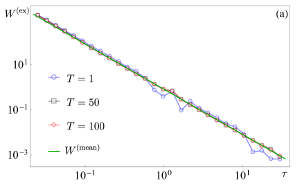
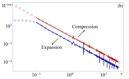
Figure 4: (a) The $\mathcal{C}/\tau^{2}$ scaling for the extra work in the finite-time adiabatic compression process. The length of the box decreases from $L_{0}=2$ to $L_{1}=1$. The exact numerical results for three initial thermal equilibrium states with temperatures $T=1,\,50,\,100$ are presented in the blue circles, black squares, and red diamonds. And the green line shows the mean extra work $W^{(\mathrm{mean})}$ in Eq. (44). (b) The extra work for the expansion and compression process. The length of the box changes from $L_{0}=2(1)$ to $L_{1}=1(2)$ for the compression (expansion) process at the temperature $T=100$. The upper red (lower blue) line with markers present the total extra work for compression (expansion) process. The markers show the exact numerical results while the line is obtained by Eq. (65).

C.4 The Engine Cycle

To optimize a finite-time Otto heat engine, we need the net work $W_{\mathrm{T}}^{\mathrm{adi}}$ and the efficiency $\eta^{\mathrm{adi}}$ for the quasi-static Otto cycle. Considering the Otto cycle given in Fig. 1(b) in the main content, the internal energy for the equilibrium state $1$ and $3$ is $\mathrm{Tr}\left[\rho_{1}H_{1}\right]=\sum_{n=1}^{\infty}p_{n}^{(1)}\tilde{E}_{n}(0)$ and $\mathrm{Tr}\left[\rho_{3}H_{3}\right]=\sum_{n=1}^{\infty}p_{n}^{(3)}\tilde{E}_{n}(1)$ with the thermal distribution $p_{n}^{(1)}=p_{n}(\beta_{h},L_{0})$ and $p_{n}^{(3)}=p_{n}(\beta_{c},L_{1})$ . For a quasi-static Otto cycle, the distribution during the quasi-static adiabatic processes remains its initial distribution, which leads to the internal energy for the state $2$ and $4$ as $\mathrm{Tr}\left[\rho_{2}H_{2}\right]=\sum_{n=1}^{\infty}p_{n}^{(1)}\tilde{E}_{n}(1)$ and $\mathrm{Tr}\left[\rho_{4}H_{4}\right]=\sum_{n=1}^{\infty}p_{n}^{(3)}\tilde{E}_{n}(0)$. We obtain the heat absorbed from the hot bath as

$$Q_{h}^{\mathrm{adi}}=\sum_{n=1}^{\infty}(p_{n}^{(1)}-p_{n}^{(3)})\tilde{E}_{n}(0),$$ (79)

and the net work as

$$W_{\mathrm{T}}^{\mathrm{adi}}=\sum_{n=1}^{\infty}(p_{n}^{(1)}-p_{n}^{(3)})\left(\tilde{E}_{n}(1)-\tilde{E}_{n}(0)\right).$$ (80)

The efficiency for the quasi-static Otto cycle follows as

$$\eta^{\mathrm{adi}}=1-r^{2}$$ (81)

with the ratio $r=L_{0}/L_{1}$. At high temperature, the summation in Eq. (80) can be approximated as

$$W_{\mathrm{T}}^{\mathrm{adi}}\approx\frac{k_{B}}{2}\left(T_{h}r^{2}-T_{c}\right)\frac{1-r^{2}}{r^{2}}.$$ (82)

For the current model with 1D quantum piston, the extra work at high temperature is

$$\Sigma_{1} =\frac{ML_{1}^{2}}{6}\left(1-r\right)^{2}\left(1+r^{2}\right),$$ (83)

and

$$\Sigma_{3}=\frac{ML_{1}^{2}}{6r^{2}}\left(1-r\right)^{2}\left(1+r^{2}\right).$$ (84)

With the explicit result of Eqs (81)-(84), the optimal control time follows as

$$\tau_{1}^{*}=\sqrt{\frac{ML_{1}^{2}\left(1-r\right)\left(1+r^{2}\right)(r^{4/3}+r^{2})}{k_{B}\left(T_{h}r^{2}-T_{c}\right)\left(1+r\right)}},$$ (85)

and

$$\tau_{3}^{*}=\sqrt{\frac{ML_{1}^{2}\left(1-r\right)\left(1+r^{2}\right)\left(r^{2/3}+1\right)}{k_{B}\left(T_{h}r^{2}-T_{c}\right)\left(1+r\right)}}.$$ (86)

And the maximal power and the EMP by Eqs. (30) and (31) is obtained as

$$P_{\mathrm{max}}^{\mathrm{Piston}}=\frac{1}{3L_{1}}\left[\frac{k_{B}\left(T_{h}r^{2}-T_{c}\right)\left(1-r^{2}\right)}{\left(M\left(1-r\right)^{2}\left(1+r^{2}\right)\right)^{1/3}\left(r^{2}+r^{4/3}\right)}\right]^{\frac{3}{2}},$$ (87)

and

$$\eta_{\mathrm{EMP}}^{\mathrm{Piston}}=\frac{2\left(1-r^{2}\right)}{3-(1-r^{2})/(1+r^{2/3})}.$$ (88)

The efficiency can be rewritten with the quasi-static efficiency $\eta^{\mathrm{adi}}$ as

$$\eta_{\mathrm{EMP}}^{\mathrm{Piston}}=\frac{2\eta^{\mathrm{adi}}}{3-\eta^{\mathrm{adi}}/[(1-\eta^{\mathrm{adi}})^{1/3}+1]},$$ (89)

which is Eq. (49) in the main content.

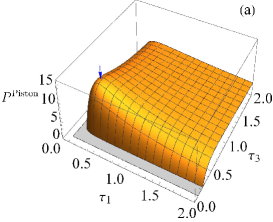
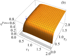
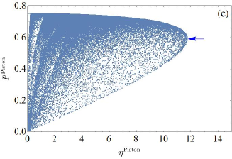
Figure 5: (a) The power and (b) the efficiency as function of the two control time $\tau_{1}$ and $\tau_{3}$ in the 1D quantum piston model. The parameters are chosen as $T_{h}=100,T_{c}=20,L_{0}=1$ and $L_{1}=2$. The power has a maximum for particular $\tau_{1}^{*}$ and $\tau_{3}^{*}$. The blue arrows gives the maximum power in subfigure (a) and the EMP in subfigure (b). (c) The achievable $(P,\eta)$ for different $\tau_{1}$ and $\tau_{3}$. The blue arrow gives the maximum power and the corresponding EMP.

In Fig. 5(a) and (b), we show the efficiency and the power for the finite-time quantum Otto cycle as functions of the control time $\tau_{1},\tau_{3}$ of the finite-time adiabatic process. Fig. 5(a) shows that the power has a maximum power at the particular control time $\tau_{1}^{*},\tau_{3}^{*}$ (marked with the blue arrow). The corresponding EMP in Fig. 5(b) is given with the blue arrow. In Fig. 5(c), we show the constraint between the power and the efficiency, by randomly choosing 600,000 pairs of $(\tau_{1},\tau_{3})$ to calculate the corresponding power and efficiency. A clear bound appears, which shows a cutoff between the power and and the efficiency. The maximum power along with the EMP is marked with the blue arrow. The detailed discussion of the exact constraint relation will be presented elsewhere.