New type II Cepheids from VVV data towards the Galactic center

Abstract

Context. The Galactic center (GC) is the densest region of the Milky Way. Variability surveys towards the GC potentially provide the largest number of variable stars per square degree within the Galaxy. However, high stellar density is also a drawback due to blending. Moreover, the GC is affected by extreme reddening, therefore near infrared observations are needed.

Aims. We plan to detect new variable stars towards the GC, focusing on type II Cepheids (T2Cs) which have the advantage of being brighter than RR Lyrae stars.

Methods. We perform parallel Lomb-Scargle and Generalized Lomb-Scargle periodogram analysis of the $K_{s}$-band time series of the VISTA variables in the Vía Láctea survey, to detect periodicities. We employ statistical parameters to clean our sample. We take account of periods, light amplitudes, distances, and proper motions to provide a classification of the candidate variables.

Results. We detected 1,019 periodic variable stars, of which 164 are T2Cs, 210 are Miras and 3 are classical Cepheids. We also found the first anomalous Cepheid in this region. We compare their photometric properties with overlapping catalogs and discuss their properties on the color-magnitude and Bailey diagrams.

Conclusions. We present the most extensive catalog of T2Cs in the GC region to date. Offsets in E($J-K_{s}$) and in the reddening law cause very large ($\sim$1-2 kpc) uncertainties on distances in this region. We provide a catalog which will be the starting point for future spectroscopic surveys in the innermost regions of the Galaxy.

1 Introduction

To investigate the central regions of the Galaxy is a top priority for studies of Galaxy evolution, since the Bulge contains $\sim$40% of the stellar mass of the Galaxy (Valenti et al. 2016; McMillan 2017). However, the Galactic center (GC) is one of the most complicated regions to study in the Milky Way because of high extinction and high crowding. At low galactic latitudes, the optical surveys such as Gaia (Gaia Collaboration et al. 2016), OGLE (Udalski et al. 1992), and ASAS (Pojmanski 1997) suffer from extreme reddening and need to be complemented with near infrared (NIR) surveys like the Two Micron All-Sky Survey (2MASS, Skrutskie et al. 2006) and the VISTA Variables in the Vía Láctea (VVV, Minniti et al. 2010; Saito et al. 2012) to detect sources in the regions of the Galactic plane where visual absorption can be as high as $A_{V}\sim$30 mag, or higher.

Over the last 10 years the synergy between OGLE and VVV has provided unprecedented results concerning variable stars in the Bulge thanks to the exploitation of their advantages and compensation for their disadvantages. In fact, OGLE scanned vast regions of the sky, generating time series with thousands of epochs, and providing the largest known catalogs of variable stars in the Bulge and Magellanic Clouds. However, the surface density of both periodic variables (RR Lyraes [RRLs], Cepheids, Miras…) and transients (microlensing events) drops dramatically at low galactic latitudes ($|b|<$1.5^∘). On the other hand, VVV could not achieve the same sky area coverage and number of epochs due to the intrinsically more telescope time-demanding observation strategies in the NIR bands. Nonetheless, its deeper images allowed the detection of Cepheids, RRLs, and microlensing events in regions where none had been found before (Dékány et al. 2013; Gran et al. 2016; Minniti et al. 2016, 2017a; Navarro et al. 2017; Majaess et al. 2018; Navarro et al. 2018; Contreras Ramos et al. 2018, henceforth, CR18), also leading to the discovery of new globular clusters (Minniti et al. 2017b, c; Bica et al. 2018). Concerning pulsating variable stars in the instability strip (IS), which are valuable standard candles since they obey period–luminosity (PL) relations, the synergy between OGLE and VVV was discussed by Pietrukowicz et al. (2012) and exploited by Bhardwaj et al. (2017b) and (Braga et al. 2018a) for type II Cepheids (T2Cs). However, since these studies were based on the OGLE lists of variables, the inner regions of the Bulge could not be inspected.

In this framework, a census of T2Cs at low latitudes is still missing. These variables are not as popular as classical Cepheids (CCs) or RRLs as standard candles. In fact, they are $\sim$2-3 mag fainter than CCs at the same period – meaning that they cannot be used to estimate distances of stellar systems outside the Local Group – but they are also much less numerous than RRLs (less than 1,000 were found in the Bulge by OGLE, while the same survey detected more than 38,000 RRLs Soszyński et al. 2014, 2017). On the other hand, T2Cs are brighter than RRLs. Moreover, the majority of the T2Cs are old ($>$10 Gyr) stars, although it was recently suggested that the W Vir (WV) subclass might partly be associated to the intermediate-age population (Iwanek et al. 2018). This means that they can also be found in stellar systems with no recent star formation events, which is a requirement to find CCs as they are purely young ($<$400 Myr, Bono et al. 2005; Anderson et al. 2016) stars. For a recent review of the properties of T2Cs, see the monography by Catelan & Smith (2015).

The aim of this paper is to find new variables in the central-most tile of the VVV survey, focusing on the detection of T2Cs. The paper is organized as follows: in Section 2, we present the data. In Section 3, we describe the light-curve analysis, including the variable star search, period determinations, and light-curve fittings. In Section 4, we discuss the classification of periodic variable stars using all tools available. We present the matches with other existing catalogs of GC variable stars in Section 5. In Section 6, we discuss the position, color-magnitude diagrams (CMDs) and Bailey (amplitude vs. period) diagrams of the final list of variables, and the obtained distances to T2Cs. Finally, the conclusions are presented in Section 7.

2 Data

Photometry — We used proprietary PSF photometric reduction (Contreras Ramos et al. 2017) of the VVV data (Minniti et al. 2010) in tile b333 (–1^∘.23¡$l$¡0^∘.23; –0^∘.46¡$b$¡0^∘.65), which covers 1.501 deg² on the GC. The camera VIRCAM has 16 chips which cover one full tile with six pointings, which are referred to as “pawprints”. Overall, the observation of each tile consists of 96 fields of view. We refer to each of these fields of view as a “pawprint-chip combination” (PCC) . The ID of each PCC is a three-digit number, where the first digit is the pawprint number, and the second and third are the chip number. We note that since there are overlaps between the different PCCs, one tile is fully covered by 48 PCCs. The advantages of PSF-fitting photometry with respect to the public aperture photometry available at VSA (http://horus.roe.ac.uk/vsa/) are manifold in crowded regions like b333, which includes the GC; it allows for blended sources to be resolved more easily, performs a better sky subtraction, and provides a deeper limit magnitude (at least $\sim$2 mag, and up to $\sim$3 mag in the most crowded regions, like b333). In principle, PSF photometry is less accurate than aperture photometry for bright, saturated sources. However, this effect is mitigated in a field like b333 for two reasons: First, because of the extreme reddening, the bright and saturated sources are statistically less frequent. Second, the aperture photometry of bright sources is performed by adopting large apertures, but the extreme crowding of b333 would hamper the results provided by this method.

Our photometric data set consists of 104 epochs in the $K_{s}$ band and two epochs in each of the $ZYJH$ bands. We consider the full $K_{s}$-band time series and the average magnitudes in the other filters.

Reddening — We adopted the 3D reddening map of Schultheis et al. (2014, henceforth S14). This map provides a 6$\times$6 arcmin grid of E(J–K) values in 21 bins of distance, from 0 to 10.5 kpc. The reddening provided by this map depends not only on the coordinates but also the distance of the target. Moreover we could not estimate the distance of all targets because not all of them are reliable distance indicators (e.g., binaries, RV Tau (RVT) stars, non-pulsating variable stars). For these variables, we have adopted the 2D map by Gonzalez et al. (2012, henceforth G12), which is independent of distance. The E($J-K_{s}$) values provided by this map are optimal for targets at the distance of the GC ($\sim$8.3$\pm$0.2[stat.]$\pm$0.4[syst.] kpc, de Grijs & Bono 2016) but are overestimated for targets closer than the GC, and vice versa (Schultheis et al. 2014; Braga et al. 2018a). To estimate the extinction $A_{ZYJHK_{s}}$ in the single bands, we adopted the reddening law of Alonso-García et al. (2017). We note that the G12 and S14 reddening maps and the adopted reddening law were obtained using VVV data. Finally, let us mention that for T2Cs, CCs, and anomalous Cepheids (ACs), we also derive independent reddening estimates by simultaneously solving the PL$H$ and PL$K_{s}$ relations for distance and reddening.

Proper motions — We adopt proper motions ($\mu_{l*}$,$\mu_{b}$) from the PSF photometry itself and $\mu_{l*}$ and $\mu_{b}$ were estimated with the same method used in Contreras Ramos et al. (2017). We note that these proper motions are relative to the Galaxy. We tried to match the targets in our final list of candidate variable stars with the Gaia DR2 (Gaia Collaboration et al. 2016, 2018) source catalog, but we found reliable matches for only 45 stars, of which only 30 have a five-parameter astrometric solution. Since these represent the minority of our sample of candidate periodic variable stars (PVSs) and parallaxes are negative for almost half of the sample, indicating an uncertain astrometric solution, we did not use these data. This was expected since Gaia performances in extremely crowded regions are not optimal.

3 Analysis of the light curves

We found 5,147,696 sources with $K_{s}$-band light curves within the tile. Such an amount of data requires proper selection to be manageable, and therefore we adopted rejection criteria at several steps of the data analysis.

3.1 Preliminary target selection

As a first step, we rejected all the sources that have light curves with either few phase points or poor-quality photometric reduction, as well as those that are considered to be nonvariable within the photometic uncertainties. More specifically, we rejected those for which a) the light curve has less than 25 phase points with a valid PSF reduction output (Gran et al. 2015; Molina et al. 2019); b) the $\chi^{2}$ of the PSF fitting (Stetson 1994) is larger than 3.5. $\chi^{2}$ , which indicates the difference between the pixel counts in the CCD and the PSF that fits the source. We noted that the sources with $\chi^{2}>$ 3.5 trace a “plume” in the sharpness ($sha$)-magnitude plane (see Fig. 1). The $sha$ parameter indicates whether the profile of the source is broader or narrower than the PSF profile, and is useful to detect nonstellar sources, which have large absolute values of $sha$; c) the difference between the maximum and the minimum magnitude of the time series $\Delta K_{s}$ is smaller than 0.1 mag. We note that this is not a cut in the $K_{s}$-band amplitude ($Amp(K_{s})$). In fact, due to the scatter of the phase points, $\Delta K_{s}$ is always larger than $Amp(K_{s})$ and the quoted cut still allows us to detect variables with $Amp(K_{s})$ down to $\sim$0.05 mag; d) the median uncertainty on the phase points is larger than 0.2 mag. We note that a magnitude uncertainty of 0.2 mag means a $\sim$20% uncertainty on the flux; and e) the variability indices based on even statistics (Ferreira Lopes & Cross 2016, 2017) indicate a nonvariable nature for the star. We did not reject saturated ($K_{s}<$12 mag, Contreras Ramos et al. 2017) stars because, although mean magnitudes and amplitudes might be inaccurate, periods are unaffected by saturation, at least for variables with $Amp(K_{s})\gtrsim$0.2 mag. Moreover, we are interested in matching our variable stars with Miras, CCs, and T2Cs found by Matsunaga et al. (2009, 2013). Their survey was shallower than the VVV due to the smaller diameter of their telescope (IRSF, 1.4m); therefore all their variables have mean $K_{s}$ magnitudes brighter than 14 mag and more than half are brighter than 12.5 mag. We discuss the offset in mean magnitude due to saturation in more detail in Section 5.5.

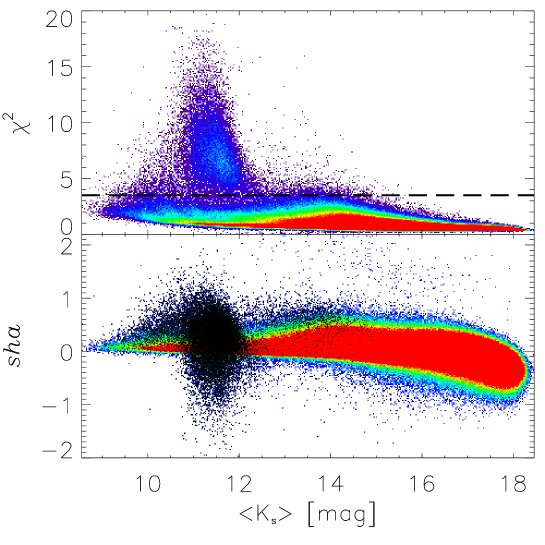
Figure 1: ${\chi}^{2}$ (top panel) and $sha$ (bottom panel) parameters as a function of $K_{s}$-band magnitude. The density map goes from blue (least dense regions of the plane) to red (densest). The thick dashed line in the top panel shows the ${\chi}^{2}$ cut applied, to reject all sources for which the photometric solution is poor. These sources are marked as black points in the bottom panel.

The quoted criteria are driven by the requirements to have enough points to obtain a solid periodogram (point a), a good photometric solution for the accuracy of the measured magnitudes (point b), an amplitude which is large enough to detect variability over noise (point c), and measured magnitudes which are more precise than 20 % (point d). In the following, we discuss point (e) in more detail.

Ferreira Lopes & Cross (2017) presented new dispersion and shape parameters for distributions with an even number of items in order to decipher whether or not the input distribution – which must be an array of observed magnitudes – could be representative of the light curve of a PVS. We note that only the measured magnitudes are taken into account, and not the epochs of observation. We have adopted the seven parameters $ED_{\sigma\mu}$, $ED_{\sigma m}$, $ED_{\mu}$, $ED_{m}$, $ED$, $ED_{(1)}$ and $ED_{(2)}$, as defined in Ferreira Lopes & Cross (2017, Table 1). To avoid ambiguity, hereafter we refer to these seven parameters as EVP_i, where $i$ ranges from 1 to 7.

As a first step, for each of the seven EVP_i in each of the 48 PCCs, we derived the modified Strateva noise models (Ferreira Lopes & Cross 2017, Eq. 18) as a function of the mean magnitude. We adopted the modified models instead of the classical ones (Strateva et al. 2001; Sesar et al. 2007) because the former better follow the distribution in the EVP_i-versus-magnitude plane, especially at bright magnitudes (see Fig. 4 in Ferreira Lopes & Cross 2017). We note that the modified Strateva models that we derived also correctly follow the distribution at faint magnitudes (see Fig. 2, although Ferreira Lopes & Cross (2017) pointed out that the modified Strateva models at faint magnitudes deviate from the distribution.

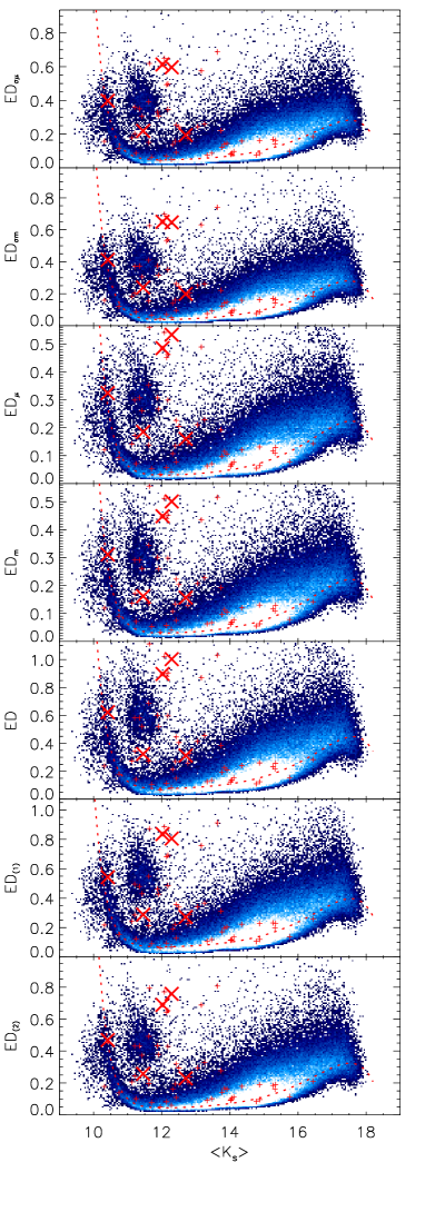
Figure 2: Density plots of the EVPs for the PCC 215. The density scale goes from dark blue (low density) to white (high density). The dashed lines represent the modified Strateva models. The red symbols display the candidate PVSs in this field of view. Small red plus symbols represent candidate PVSs with ambiguous or uncertain classification, and large red crosses represent candidate PVSs with reliable classification (see Section 4).

For each of the EVP_i, we calculated $I_{(P)i}$, as defined in Ferreira Lopes & Cross (2017, Eq. 19). By construction, $I_{(P)i}<1$ indicates a nonvariable star according to the $i$-th EVP. One may also take account of the seven EVPs altogether and reject – as nonPVSs – all the targets for which the sum of the $I_{(P)i}$ ($\Sigma I_{P}$) is less than seven. W note that this is possible because for a given target the seven $I_{(P)i}$ are all of the same order of magnitude. However, we have empirically checked that there are some bona fide PVSs – especially those with small amplitudes – for which $\Sigma I_{P}<7$ (see Fig. 2 which shows that several candidate PVSs are below the $I_{(P)i}=1$ locus.). Therefore, we decided to adopt a more conservative approach and we kept, as candidate PVSs, all the targets for which $\Sigma I_{P}>3.3$. This threshold was chosen as a compromise between a moderate increase of false alarms and a higher completeness.

3.2 Preliminary phase point selection

After the rejection based on the criteria $a)$, $b)$, $c)$, $d)$ and $e)$ in Section 3.1, where $\sim$15% of the sources were discarded, for each light curve we performed a rejection of the phase points that we assumed to be outliers. The rejection process was based on an iterative sigma clipping at a 3.5$\sigma$ level with respect to the median magnitude. This is a conservative threshold that allowed us to detect periodic variable stars with large amplitudes (up to $\sim$2 mag) and at the same time to discard outlying phase points that could affect the accuracy of the periodicity search. In this step, for $\sim$57% of the light curves, we do not reject any phase points. For $\sim$23%, $\sim$10%, $\sim$5%, and $\sim$2% of the light curves, the number of points that were rejected was one, two, three, and four, respectively. For the remaining $\sim$3% of the light curves, five or more points (up to eighteen) were rejected.

3.3 Periodicity search

After the selections and cuts described in the above section, we ran our periodicity search algorithm over all the light curves. As a preliminary step, we converted our epochs from Julian dates into heliocentric Julian dates ($t_{HJD}$). We calculated both the classical Lomb-Scargle (LS; Scargle 1982) and the Generalized Lomb-Scargle (GLS; Zechmeister & Kürster 2009) periodograms. The difference between the two is that the zero point of the model function in the LS is fixed at the empirical mean magnitude of the phase points, while in the GLS method, the zero point is allowed to float. Therefore, the GLS is more reliable when the light curve is not well sampled (VanderPlas & Ivezić 2015).

We performed both a LS and a GLS analysis because the comparison of the periodograms is useful to detect and automatically reject stars that are not periodic variables. We have verified empirically that, if the highest peak of the GLS periodogram does not match – within the typical peak width – any among the ten highest peaks of the LS periodogram, the peaks are associated with light variations that are not strictly periodical, and therefore we can reject the target as a nonPVS. In the following sections, we explain the details of our analysis.

3.3.1 Frequency grid

To calculate the periodograms, we used an evenly spaced grid of frequencies, from $\nu_{min}$=$\dfrac{1}{\Delta t}$ days^-1 – where $\Delta t$ is the total time between the first and the last epoch of the light curve in days – to $\nu_{max}$=0.995 days^-1. This range was chosen based on the following considerations. 1) Our first aim is to detect T2Cs and fundamental-mode (FU) CCs, which have periods from $\sim$1 to $\sim$200 days. 2) We did not include frequencies that are too close to 1 day^-1 because the increase in the number of genuine variables would come at the cost of a much higher increase of aliases around 1 day. Based on the typical number of phase points for our light curves, the limit at 0.995 days^-1 allows us to automatically reject most of the aliases. 3) We did not extend $\nu_{max}$ to the range of frequencies of RRLs because the computation time would be around ten times longer with $\nu_{max}=5$ days^-1. Although the limit at $\nu_{max}$ might generate aliases, we adopted an a posteriori LS analysis on a much smaller sample to solve the aliases (see Section 3.4.3).

The number of points in the frequency grid of the periodogram ($N_{freq}$) depends on the range of epochs covered by the light curve ($\Delta t$). As a matter of fact, $Df=\Delta t^{-1}$ is the characteristic width of a peak in the periodogram. Therefore, we set $N_{freq}=int(n_{spp}\cdot\Delta t\cdot(\nu_{max}-\nu_{min}))$, where $n_{spp}$ is the oversampling factor (Graham et al. 2013) and $n_{spp}$ corresponds to a phase shift of about 0.1 between neighboring frequencies that ensure the signal detection of almost all variable types (for more detail see Ferreira Lopes et al. 2018). We set $n_{spp}=9$ for all the light curves (normally, the recommended value of $n_{spp}$ is between 5 and 10; VanderPlas & Ivezić 2015). Since $\Delta t$ is not the same for all the light curves, $N_{freq}$ ranges between $\sim$3,000 and $\sim$16,600, with a mean of 16,082.

3.3.2 Height of the peaks and frequency aliases

After obtaining the periodograms, we empirically verified that if the peaks are not high enough or if there are too many low peaks – see details below – then the light curve is too noisy to properly classify our targets.

Therefore, we perform a further selection of targets based on the intensity of the peaks of the periodograms. Adopting the standard deviation of the periodogram itself ($\sigma_{P}$), we discarded 1) light curves with less than 30 points and no peaks higher than 8$\sigma_{P}$; 2) light curves with 30 points or more, and no peaks higher than 9$\sigma_{P}$; and 3) light curves with more than 140 peaks higher than 5$\sigma_{P}$ and no peaks higher than 12$\sigma_{P}$.

After this further selection, we adopted a procedure to check—and eventually correct—aliased frequencies. Following VanderPlas & Ivezić (2015) and VanderPlas (2018), we have checked whether the frequency of the highest peak ($\nu_{hi}$) is either a harmonic of the fundamental frequency, an alias, or the true fundamental frequency. This is done in two steps. First, we checked whether or not there were sufficiently high peaks (larger than 6 or 7$\sigma_{P}$ if the number of phase points is, respectively, smaller or larger than 30) around the critical frequencies ($\nu_{check}$). To check for harmonics, $\nu_{check}=\dfrac{\nu_{hi}}{m}$, with $m$=2,3; to check for aliases, $\nu_{check}=|\nu_{hi}+n\cdot\nu_{alias}|$, where $\nu_{alias}$=1 day^-1 and $n$=$\pm 1,\pm 2$. Second, we compared the $\chi^{2}$ of the Fourier fits at $\nu_{hi}$ and $\nu_{check}$, and selected the best frequency as that which minimizes the $\chi^{2}$.

Finally, we obtained best frequency estimates for 889,663 targets, of which 435,126 and 454,537 are from GLS and LS periodograms, respectively.

We folded the light curves calculating the phases $\phi$ as the decimal part of $\dfrac{t_{HJD}-T_{0}}{P_{best}}$, where $T_{0}$ is an arbitrary zero epoch that we set at 0.0 days.

3.4 Light-curve fit

Despite the quoted cuts and selections, after the analysis of the periodograms, we still have almost one fifth from the original sample. Therefore, further selections are needed to narrow down the final sample to PVSs only.

For this purpose and to derive the pulsation properties of the targets (mean magnitude, amplitude, and uncertainties), we fitted the folded light curves with a Fourier series of the second order ($F(\phi)$), and used the properties of the fit to select our candidate variable stars. We use the second order because, at this stage, the sample of light curves is still not completely free from nonPVSs, and Fourier series of higher order would provide unreliable fits with unphysical bumps.

3.4.1 Mean magnitudes and amplitudes

After obtaining the Fourier fit of the light curves, we derived the mean magnitudes $\langle K_{s}\rangle$ as the integral of the fits converted to flux, and the amplitudes $Amp(K_{s})$ as the difference between the brightest and the faintest points of the fits. We estimated the uncertainties on the mean magnitude ($eK_{s}$) as the sum in quadrature of the standard deviation of the phase points around the fit plus the median photometric error on the phase points. The uncertainty on the amplitude $eAmp(K_{s})$ was derived as the sum in quadrature of the median photometric errors of the phase points around the maximum and minimum, plus the standard deviation of these phase points around the fit of the light curve. The final value was weighted with the number of phase points around the maximum and the minimum (Braga et al. 2018c). The fits might show, at most, two secondary minima and maxima. In this case, we estimate the amplitude of the bump $Amp(K_{s(bump)})$ as the difference between the secondary minimum and maximum.

3.4.2 Selection of the final sample

With almost 900,000 targets remaining, we applied further selections aimed to narrow down the sample to a more manageable size.

1) Selection on phase gaps — A fraction of folded light curves display wide gaps in phase ($\geq$0.25 cycles). We empirically checked that for stars with $P_{best}\leq 330$ days, these gaps are caused by a poor estimate of $P_{best}$ and that the target is not a PVS. Therefore, we reject all targets with a phase gap wider than 0.25 cycles and $P_{best}\leq 330$ days. Targets with wide gaps but longer periods are kept in the sample of candidate PVSs because bona fide PVSs with long periods also show such gaps, caused by the 1 year alias.

2) Selection on amplitude — We put an upper limit of $Amp(K_{s})\leq$3.5 mag on the light amplitude. This is a very conservative upper limit for the light amplitudes of Miras, which are the variables with the largest amplitudes among those that we are interested in. This threshold is based on photometric surveys of Miras in the Bulge, both in the NIR (Matsunaga et al. 2009, which does not find any Mira with $Amp(K_{s})\;\lower 2.58334pt\hbox{$\sim$}\kern-6.7pt\raise 1.72218pt\hbox{$>$}\;$2.7 mag), and in the optical (Soszyński et al. 2013, which does not find any Mira with $Amp(I)\;\lower 2.58334pt\hbox{$\sim$}\kern-6.7pt\raise 1.72218pt\hbox{$>$}\;$7 mag; we note that for Miras we can assume a ratio $Amp(K_{s})$/$Amp(I)\approx$ 0.45, Whitelock 2012). Moreover, the accuracy and precision of our data do not allow to detect PVSs with $Amp(K_{s})<0.03$ mag (Gran et al. 2015). Therefore, we only keep the targets with 0.03 $\leq Amp(K_{s})\leq$ 3.5 mag.

3) Selection on bumps — Second-order Fourier fits might show local minima and maxima. Although some variables of the IS do show these features, they are not particularly deep, especially at long wavelenghts (Laney & Stobie 1993). Therefore, if $\dfrac{Amp(K_{s(bump)})}{Amp(K_{s})}>0.15,$ which means that the fit displays a deep bump, we discard the target because these features in the light curve fit show up in noisy or nonperiodic light curves.

4) Selection on template fit — Templates of NIR ($JHK_{s}$) light curves of T2Cs are available (Bhardwaj et al. 2017a). For all targets with 1 day $\leq P_{best}\leq$ 80 days, we derived the template fit of the light curve. We note that we did not properly apply the template procedure to find the mean magnitude because this would require the knowledge of the epoch of maximum light. We performed a least-squares minimization of the template function $T(\phi)$ with respect to three independent variables, which are the shift in magnitude ($\Delta mag$), the shift in phase ($\Delta\phi$), and the amplitude of the template fit $AK_{s[T(\phi)]}$. We note that in this process the shape of the template fit is fixed. Therefore, the least-squares minimization process only shifts the fitting function horizontally, vertically, or stretches its amplitude. We subsequently compare the template fit and the Fourier fit. If they are similar, this means that the target can be considered as a candidate T2C. Therefore, we compute a parameter ($c_{10}$) to quantitatively compare the two fits, defined as the average of the absolute value of the difference between the two fits, divided by the average amplitude of the two fits: $c_{10}=\dfrac{\langle|F(\phi)-T(\phi)|\rangle}{(AK_{s[F(\phi)]}+AK_{s[T(\phi)]})/2}$. If $c_{10}>0.2$, the two fits are quite different from one another, therefore we can discard the target from the list of candidate PVSs. We note that 0.2 is a conservative threshold that allows for targets that are plainly not PVSs to be rejected, but also allows us to keep eclipsing binaries (EBs) with light curves that are quite different from those of T2Cs. Taking account of the accuracy of our data, we can assume that the shape of the light curves of CCs is similar to those of T2Cs. We tried to fit the light curves using also the templates of CCs (Inno et al. 2015), trying to separate between T2Cs and CCs, based on the ${\chi}^{2}$ of the two fits. However, this was not possible because the two templates are very similar over the whole range of periods. As a matter of fact, for the majority of our light curves (all those with $\langle K_{s}\rangle\;\lower 2.58334pt\hbox{$\sim$}\kern-6.7pt\raise 1.72218pt\hbox{$>$}\;$ 14.5 mag) the ${\chi}^{2}$ of the two fits are often similar. Figure 3 shows the light curve of a variable which is clearly a T2C (based on both its location in the Bailey diagram and its proper motion) despite the $\chi^{2}$ of the T2C template fit being larger than that of the CC template fit (see labels).

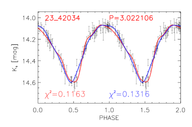
Figure 3: Light curve of the variable star b333_23_42034, a T2C. The name and the period (in days) are labeled on the top. The red and blue lines display the CC and the T2C template fits, respectively. The ${\chi}^{2}$ of the two fits are labeled at the bottom. The colors of the labels are the same as those of the fits.

5) Selection and ranking on modified ${\chi}^{2}$ — A further selection is based on the dispersion of the phase points around the fit. However, we did not compute a simple ${\chi}^{2}=\dfrac{{\Sigma}_{i}(mag_{i}-F(\phi_{i}))^{2}}{n}$, where $mag_{i}$ is the measured magnitude of the $i$-th phase point and $F(\phi_{i})$ is the value of the Fourier fit at the phase $\phi_{i}$ of the $i$-th phase point. We adopted a modified chi squared ${\chi_{A}}^{2}={\chi}^{2}/{Amp(K_{s})}^{2}$ that we also used to rank our final sample of targets for the visual inspection, from the “clearest” (smaller ${\chi_{A}}^{2}$) to the “least clear light” curves. The division by the squared amplitude has the effect of increasing the ${\chi_{A}}^{2}$ of the small-amplitude variables and in turn decreasing their rank. This operation is needed to obtain a more reliable ranking: Figure 4 shows two variables that have an identical ${\chi}^{2}$ but different $Amp(K_{s})$. Based on ${\chi_{A}}^{2}$, the variable in the upper panel is ranked higher than the one in the bottom panel to take account of the relative dispersion with respect to the amplitude. Finally, we rejected all the targets for which ${\chi_{A}}^{2}>0.2$.

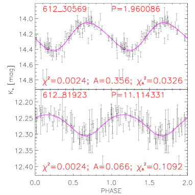
Figure 4: Top: Light curve of the variable _612_30569. The name and period (in days) are labeled at the top. The Fourier fit is displayed as a magenta line. The ${\chi}^{2}$, $Amp(K_{s})$ and ${\chi_{A}}^{2}$ are labeled at the bottom. Bottom: As in the top panel, but for _612_81923.

6) Visual inspection — After the quoted steps, we were left with 54,667 targets, which is a little more than 1% of the starting sample. This is still too large and contains many stars that cannot be considered as bona fide candidate PVSs. We performed a visual inspection and found 1,013 “top tier” candidates. We note that the final catalog includes 1,019 targets because we manually added six Cepheids already found in the literature (Matsunaga et al. 2011, 2013) which are present in our initial target list but were not retrieved by the periodicity search algorithm (see Section 4 and  5.3).

3.4.3 Refining the periods and fits

After the quoted selections it is possible to visually inspect the light curves of all the candidate variables to improve our analysis. As a matter of fact, these steps are mandatory for a more accurate classification of the PVS candidates.

1) Unresolved aliases — The alias check process performed in Section 3.3.2 has one disadvantage: it does not detect aliases at frequencies outside the frequency grid (in our case, for $\nu>0.995$ days^-1). Therefore, we repeated the whole periodicity search process with LS and GLS on the 1,019 PVS candidates, but this time on a frequency grid going from $\nu_{min}$=0.000 days^-1 to $\nu_{max}$=5 days^-1. Since the size of this sample is much smaller than the starting list of sources, this is not a time-consuming process. For 77 targets, we found a $P_{best}$ shorter than 1 day, which is different from that obtained in the first iteration.

2) Order of the Fourier fit — Some variables – especially the brightest ones, which have small photometric errors – show well-defined light curves with low noise, and are better fitted by Fourier series of an order higher than the second. For these variables, we repeated the fit using a third-, fourth-, or fifth-order Fourier series. We also repeated the fits of almost sinusoidal light curves using a first-order Fourier fit to avoid unphysical bumps appearing especially in light curves with few phase points.

3) Frequency doubling — EBs, RVTs, but also WVs with periods down to $\sim$16 days (Soszyński et al. 2017) might have light curves with alternating deep and shallow minima of light. For these targets, our algorithm for the periodicity search incorrectly assigned $P_{best}$ to the time interval between two adjacent minima. However, this is half of the true, physical variability period. To detect the alternating minima and to better classify the variables, we visually inspected the light curves of all the PVS candidates at both $P_{best}$ and 2$\cdot P_{best}$. We changed $P_{best}$ into 2$\cdot P_{best}$ for those variables with clear signs of alternating minima.

4 Classification

The stars in our final sample have periods between $\sim$0.38 and $\sim$1240 days. In principle, they could be of any type among the pulsating stars, that is, RRLs, T2Cs, CCs, ACs, long-period variables (LPVs, which include Miras and SRVs, but not OSARGs, which have overly small amplitudes; Wray et al. 2004), non-pulsating variables (NPVs), which include, for example, EBs of any kind (detached, semi-detached, W UMa contact), and spotted stars, that is, stars which show variability due to the interplay of their rotation and the presence of large spots on their surface. Normally, these objects are associated to the pre-main sequence population. To discriminate between these types of variables, we adopted the criteria listed below. We point out that none of the following criteria were adopted alone for the classification, but they were all considered together. We list them in order of decreasing reliability.

1) Periods — Based on the literature, we adopted period thresholds for the quoted types of variables (see Table 1). We adopted conservative limits because the period thresholds of pulsating stars depend on many factors (metallicity, helium abundance, $\alpha$ enhancement) and a detailed summary is beyond the aim of this paper. 1a) NPVs — These variables cover a wide range of periods, which includes all the periods of our targets. 1b) RRLs — Using OGLE data, Soszyński et al. (2014) found more than 38,000 RRLs, which is the largest homogeneous available catalog of RRLs. The period ranges of RRc and RRab are [0.20-0.54 days] and [0.28-1.00 days], respectively. These are quite usual thresholds, apart from the lower limit of RRab, for which $\sim$0.4 is a more common value. However, since the shortest period in our list of PVSs is $\sim$0.38 days, there is no difference in adopting one or the other value for the threshold. 1c) ACs — The most extensive catalog of bona fide ACs is provided by the OGLE survey Soszyński et al. (2015), for targets in the Large Magellanic Cloud (LMC) and Small Magellanic Cloud (SMC). These latter authors found ACs in a period range which is wider (0.38-2.7 days) than those quoted in theoretical studies ($\sim$0.5-2 days Fiorentino et al. 2006). We point out that the GC is an environment which in principle does not favor the formation of ACs, which arise either from very metal-poor or binary progenitors (Fiorentino & Monelli 2012). Nonetheless, to date, 20 of them were found in the Bulge (Soszyński et al. 2017). Therefore, we cannot discard a priori the possibility of finding ACs. 1d) CCs — The sample of CCs with the widest range in period (0.25-208 days) is that of LMC and SMC CCs by OGLE (Soszyński et al. 2008a, 2010). We point out that the adopted empirical ranges are wider than theoretical predictions (Bono et al. 2000). 1e) T2Cs — The commonly accepted lower limit of the periods of T2Cs – which marks their separation from RRLs – is 1 day (Di Criscienzo et al. 2007). To set an upper threshold for T2Cs is a more delicate issue. RV Tau stars are the longest-period T2Cs and might show alternating deep and shallow minima. Therefore, two periods can be defined: the time passing between two deep minima (true period) and the time between two adjacent minima (formal period, by definition, half of the fundamental period). According to Wallerstein (2002), the maximum formal period is theoretically $\sim$75 days. On the observational side, the longest formal periods in T2C catalogs are shorter than 90 days for Galactic globular clusters (Matsunaga et al. 2006, IRSF) and shorter than 80 days for the LMC, SMC, and Bulge (Soszyński et al. 2017, 2018, OGLE). However, it is not easy to detect the alternating minima, therefore it is not straightforward to discriminate between the two periods. Finally, we adopted a conservative threshold of 100 days for the formal period. 1) Miras — These variables are often classified based on their amplitude ($A_{I}$¿0.8 mag) rather than their period. The most common lower period limit in the literature is 100 days (Ita & Matsunaga 2011; Catchpole et al. 2016). Nonetheless, Miras with shorter periods – down to $\sim$80 days – were found in the Galactic Bulge (Soszyński et al. 2013) and furthermore Whitelock (2012) states that Miras could have periods shorter than 100 days. Therefore, we adopt 80 days as our threshold. We note that this is also the lower limit given in the General Catalog of Variable Stars (Samus’ et al. 2017) and the International Variable Stars Index definition of the class. On the other hand, the periods of Miras can be as long as 2000 days Whitelock (2012), which is longer than the longest period in our final sample of candidates.

Table 1: Table of criteria for the classification of variable stars.

Type	$P_{min}$	$P_{max}$	Ref.	PL$H$	PL$K_{s}$	Ref.
	days	days	mag	mag
NPSs	¡0.38	¿1000	1	…	…	…
RRc(FO)	¡0.38	$\sim$0.54	2	…	–1.56–2.72$\cdot\log P$	11
RRab(FU)	$\sim$0.38	$\sim$1	2	–0.971–2.226$\cdot\log P$	–0.998–2.250$\cdot\log P$	11
ACFO	$\sim$0.38	$\sim$1.2	3	…	–2.42–4.18$\cdot\log P$	12
ACFU	$\sim$0.50	$\sim$2.7	3	…	–1.74–3.54$\cdot\log P$	12
CCFO	¡0.38	$\sim$6.3	4,5	–2.851–3.455$\cdot\log P$	–2.890–3.455$\cdot\log P$	13
CCFU	$\sim$0.80	$\sim$210	4,5	–2.366–3.227$\cdot\log P$	–2.408–3.245$\cdot\log P$	13
T2C	$\sim$1	$\sim$100	6,7,8	–3.358–2.202$\cdot\log P$	–3.418–2.232$\cdot\log P$	14
Miras	$\sim$80	$\sim$2000	9,10	…	–6.865–3.555$\cdot\log P$	15

2) Bailey diagram — We have collected the periods and $Amp(K_{s})$ of RRLs, T2Cs, CCs, Miras and ACs in the literature, in the field of the Milky Way, the LMC, the SMC, the Galactic Globular Clusters and the Galactic Bulge (Matsunaga et al. 2006, 2013; Ripepi et al. 2014; Inno et al. 2015; Ripepi et al. 2015; Gran et al. 2016; Matsunaga et al. 2016; Ripepi et al. 2016; Yuan et al. 2017). For each candidate PVS, we have checked its position in the Bailey diagram and compared this with the position of variables of known type, to narrow down the classification.

3) Distance and position — Based on known calibrations of PL relations for the different types of variables (see Table 1), for each target, we have calculated a set of provisional distances: $d_{RRab}$, $d_{RRc}$, $d_{CCFO}$, $d_{CCFU}$, $d_{ACFO}$, $d_{ACFU}$, $d_{T2C}$, $d_{Mira}$. These must be interpreted as the distance at which the target would be located if it was a variable of a given type, as in the subscript. Using the ($l$,$b$) coordinates, we also derive the provisional positions in Cartesian coordinates—$x$, $y$ and $z$—of the targets in the Galaxy. We note that there are several caveats on distance. 3a) Metallicity dependence — At NIR wavelenghts, the effect of metallicity on the PL relation of CCs is reduced compared to the optical (Marconi et al. 2010; Bhardwaj et al. 2015). The effect of metallicity is negligible also on the PLs of T2Cs (Di Criscienzo et al. 2007) and Miras (Whitelock et al. 2008). There is no solid theoretical or empirical evidence of metallicity dependence of the PL$K_{s}$ of ACs (Fiorentino et al. 2006) either. On the other hand, the zero-point of the PL$K_{s}$ relation of RRLs is affected by metallicity (Bono et al. 2001; Catelan et al. 2004; Marconi et al. 2015). We assume [Fe/H]=–1.0 (Sans Fuentes & De Ridder 2014; Hajdu et al. 2018) as a typical iron abundance of Bulge RRLs. We note that the error propagation associated to the uncertainty on [Fe/H] is negligible compared to the other factors. 3b) RVTs — There is currently debate over whether RVTs follow the PL relation of T2Cs (Matsunaga et al. 2006; Bhardwaj et al. 2017a) or not (Wallerstein 2002; Ripepi et al. 2015). More specifically, it is not clear how to separate intermediate-age RVTs from old, low-mass RVTs, which have a completely different evolution; it might be appropriate to give them a different name (e.g., V2342 Sgr stars, Catelan & Smith 2015). To sum up, the distances of even bona fide RVTs cannot be trusted. 3c) Reddening — We are aware that the pixels of the S14 reddening map are too large to provide accurate E($J-K_{s}$) estimates of targets within a region where the reddening pattern is so irregular at small scales. In Section 5.5, we discuss in more detail the comparison of reddening and distance with other works. We point out that for a fraction of targets our distance estimates might be overestimated due to underestimated extinction. However, NIR multi-band light curve templates are available for RRLs, CCs, and T2Cs (Braga et al. 2018b, Inno et al. 2015 and Bhardwaj et al. 2017a, respectively), providing the possibility to estimate accurate $J$- and $H$-band mean magnitudes ($\langle J\rangle$, $\langle H\rangle$) and, in turn, to derive independent distance and $A_{Ks}$ estimates. This is the same approach used by M09 and M13, who did not use any reddening map. We point out that although we did derive $\langle J\rangle$, we only employed PL$K_{s}$ and PL$H$ relations to estimate extinction and distances, because differential reddening and variations of the reddening law have an overly large effect on targets in this region. The net effect of employing the PL$J$ relations is to increase distances by $\sim$0.4 kpcs, leading to a very unlikely peak of T2C distances around $\sim$8.9 kpc.

To estimate the $\langle J\rangle$ and $\langle H\rangle$ of RRLs and CCs, we used the light-curve templates of RRLs (Braga et al. 2018b) and CCs (Inno et al. 2015). For T2Cs, only the $K_{s}$-band light-curve templates are available. However, they provide accurate mean magnitudes also when applied to the $H$-band data (Bhardwaj et al. 2017a), since the light-curve morphology in these two bands is very similar. Finally, we adopted the $J$-band CCFO light-curve template by (Inno et al. 2015) to derive $\langle J\rangle$ for T2Cs. We checked that, within the photometric errors, no difference is seen when using the phase correction (Bhardwaj et al. 2017b).

To perform the fits, one must rescale the amplitude using the $Amp(J)/Amp(K_{s})$ and $Amp(H)/Amp(K_{s})$ amplitude ratios. For RRLs and CCs, we adopted the ratios provided by Braga et al. (2018c) and Inno et al. (2015), respectively. For T2Cs, we checked that both $Amp(J)/Amp(K_{s})$ and $Amp(H)/Amp(K_{s})$ are equal to one, within the uncertainties, using globular cluster data from Matsunaga et al. (2006). Furthermore, we verified that minor phase shifts between the $J$, $H,$ and $K_{s}$ light curves are negligible ($<$0.05 pulsation cycles). Therefore, the $J$- and $H$-band template fits were performed by leaving only the mean magnitude as a free parameter. Figure 5 shows the use of the template for an RRab (left), T2C (center), and CC (right). Computing $\langle J\rangle$ and $\langle H\rangle$ based on the intensity integral over the template provides mean magnitudes that are more accurate than the simple average of the two epochs, and this is even more critical when the $J$- or $H$-band data are sampled around the minimum.

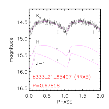
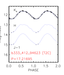
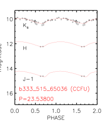
Figure 5: Left: Phased $J$-, $H$-, and $K_{s}$-band light curves of a RRab over which we applied the light-curve template. The ID, type, and period of the star are labeled in red. Center: As in left, but for a T2C. Right: As in left, but for a CCFU.

We point out that due to the high extinction, not all of the candidate variables have $JH$-band data with acceptable photometric errors ($<$0.2 mag). This means that we could not apply the PL$HK_{s}$ method to all of them. More precisely, we lack precise $J$-band data for 16 T2Cs and $H$-band data for 8 T2Cs and 1 CCFU.

To sum up, for 2 CCs, 5 RRabs, and 156 T2Cs, we derived two sets of distances and extinctions which we labeled $d_{S14}$, $A_{Ks(S14)}$, and $d_{PL}$, $A_{Ks(PL)}$, respectively, for those derived using the S14 reddening map and those obtained with the PL$HK_{s}$ method.

4) Velocity — We use the provisional distances found before to derive provisional transverse velocities, using $v_{t}=4.74\cdot d\cdot\mu$, where $d$ is in kiloparsecs, $\mu$ in mas/yr and $v_{t}$ in km/s. We note that to derive the direction and intensity of the tangential velocity, we summed the proper motion of Sgr A* (Reid & Brunthaler 2004) and our own proper motions. According to Braga et al. (2018a) we assume that this operation provides a proxy of absolute proper motions. We did not correct for the peculiar motion of the Sun because we are interested in understanding whether our targets follow the rotation curve of the Galactic disk, both on our side and on the far side of it. We assume, as a threshold on the reliability of $\mu$, a combined statistical error ($CSE=\sqrt{err\mu_{l*}^{2}+err\mu_{b}^{2}}$) of 2 mas/yr, as did Contreras Ramos et al. (2017), who used the same data. We also use the direction of $v_{t}$ as a diagnostic to discriminate between types of Cepheids belonging to different Galactic populations (e.g., we assume that the motion of CCs and young variables must be disk-like). We did not include radial velocities ($v_{r}$) in our analysis for two reasons. First, $v_{r}$ from the APOGEE survey (Majewski et al. 2017) are available for only seven of our targets. Second, and most important, with the exception of EBs and NPVs, our targets are radially pulsating stars, with radial-velocity amplitudes of the order of tens of kilometres per second (Bono et al. 2000; Feast et al. 2008) due to the inflation and deflation of the layers where absorption lines originate. Therefore, a single $v_{r}$ measurement is not an accurate estimate of the radial velocity of the barycenter of the star.

5) Dereddened $H-K_{s}$ color — Generally, our dereddened colors have large uncertainties (the peak of the distribution of $(H-K_{s})_{0}$ is at $\sim$0.3 mag), which also increase after the dereddening. Moreover, while we have accurate estimates of $\langle K_{s}\rangle$, this is not true for other bands. Finally, since the reddening is extremely severe, we can only rely on the $H-K_{s}$ color, which covers a very small wavelength range. Nonetheless, $(H-K_{s})_{0}$ comes in handy to separate between Miras and long-period CCs, since the former are  $\sim$$>$ 0.5 mag redder (Matsunaga et al. 2009, 2013).

6) Shape of the light curve — Although in the NIR many features of the light curves present in the optical are smoothed, it is still possible, by visually inspecting the light curves, to refine the classification of, for example, detached EBs (DEBs), which have narrow, alternating deep and shallow minima between almost flat plateaus.

Table 2: Properties of the candidate PVS.

ID	sat	Literature ID	$RA$	$DEC$	type	$P_{best}$	$Z$	$Y$	$J$	TJ	$H$	TH	$\langle K_{s}\rangle$	$Amp(K_{s})$	$\mu_{l*}$	$\mu_{b}$	$A_{Ks}$	$d$	$v_{t}$
			deg	deg		days	mag	mag	mag		mag		mag	mag	mas/yr	mas/yr	mag	kpc	km/s
b333_59_98743			265.765256	–28.941707	96	0.387960	20.132$\pm$0.114	18.622$\pm$0.032	16.873$\pm$0.023		15.547$\pm$0.030		14.770$\pm$0.047	0.252$\pm$0.049	0.31$\pm$1.87	–5.12$\pm$1.65	…	…	…
b333_46_54772			265.725409	–29.200448	9	0.406797	20.797$\pm$0.117	18.752$\pm$0.059	16.909$\pm$0.014		15.331$\pm$0.015		14.403$\pm$0.027	0.190$\pm$0.026	–2.45$\pm$0.55	–0.70$\pm$0.80	…	…	…
b333_16_24211			265.689600	–29.489227	469	0.442667	17.950$\pm$0.018	16.163$\pm$0.011	14.622$\pm$0.008		13.378$\pm$0.015		12.567$\pm$0.018	0.141$\pm$0.018	–2.10$\pm$0.42	–1.11$\pm$0.36	…	…	…
b333_29_10464		OGLE-BLG-ECL-069715	265.506766	–29.000586	A	0.505139	14.058$\pm$0.005	13.593$\pm$0.008	13.126$\pm$0.007		12.805$\pm$0.010		12.482$\pm$0.017	0.148$\pm$0.016	–4.21$\pm$0.40	–1.98$\pm$0.36	…	…	…
b333_38_13973			266.087807	–29.593169	469	0.505688	…	20.514$\pm$0.159	18.547$\pm$0.059		16.530$\pm$0.035		15.185$\pm$0.041	0.260$\pm$0.043	–6.64$\pm$1.59	–1.12$\pm$1.50	…	…	…
b333_414_55144		[MCZ2016]_VVV-RRL-55144	266.104489	–28.659180	5	0.508390	…	…	17.936$\pm$0.083	*	15.829$\pm$0.054	*	14.635$\pm$0.043	0.406$\pm$0.047	–11.57$\pm$1.63	2.67$\pm$1.88	1.33	5.34$\pm$0.24	300$\pm$32
b333_511_117170			266.345607	–29.183243	95	0.515417	…	20.243$\pm$0.294	…		17.946$\pm$0.177		16.031$\pm$0.128	0.257$\pm$0.128	–8.92$\pm$5.74	–3.56$\pm$3.80	…	…	…
b333_25_81044			265.468647	–29.324717	59	0.517853	…	21.041$\pm$0.442	19.758$\pm$0.129		17.007$\pm$0.055		15.505$\pm$0.065	0.274$\pm$0.065	–1.69$\pm$2.18	–1.94$\pm$1.98	…	…	…
b333_53_12695			265.773550	–29.685386	A5	0.524798	…	…	18.228$\pm$0.049		16.372$\pm$0.034		15.265$\pm$0.048	0.306$\pm$0.051	–3.17$\pm$1.74	0.52$\pm$1.67	…	…	…
b333_44_75303			266.006268	–29.936152	94	0.525078	19.394$\pm$0.047	17.550$\pm$0.016	15.904$\pm$0.011		14.403$\pm$0.014		13.278$\pm$0.028	0.190$\pm$0.027	–2.63$\pm$0.55	0.21$\pm$1.28	…	…	…

We provide the light curves of these 1,019 candidate variables in Table 3.

Table 3: $K_{s}$-band time series of our candidate variables.

Name	HJD–2,400,000	Mag	Err
	days	mag	mag
b333_59_98743	55844.02155	14.704	0.043
b333_59_98743	55423.14904	14.607	0.040
b333_59_98743	55777.13660	14.865	0.054
b333_59_98743	55778.19837	14.627	0.032
b333_59_98743	55794.12621	14.657	0.047
b333_59_98743	55806.15221	14.674	0.046
b333_59_98743	55820.10395	14.705	0.045
b333_59_98743	55830.02354	14.807	0.044
b333_59_98743	55849.02315	14.518	0.036
b333_59_98743	55987.37349	14.730	0.052

After taking account of the quoted criteria, we assigned a variable type to each of the candidate PVSs in the final sample. We ended up with unambiguous classification for 472 variables (5 RRab, 164 T2Cs, 3 CCFU, 1 ACFU, 16 SRVs, 210 Miras and 73 NPVs, of which 47 DEBs, see Table 2, second column). For the other 547 variables, we could not provide a solid classification due to uncertainties on the reddening and distance, and due to noisy light curves. More specifically, for 99 of them, the light curve is clear enough to be classified as “high-rank” candidate variables. However, due to the lack of other information, or ambiguity in the criteria listed above, we could only provide a tentative classification (e.g., 96 in the fifth column in Table 2 means that we are uncertain on whether b333_509_98743 is a RRc or a NPV). For the remaining 448 candidate PVSs, the light curve was not clear enough (due to noise, high photometric error, or secondary modulations), and therefore they were classified as “low-rank variables”. These too have to be considered as variables without a certain classification.

We point out that we have found the first bona fide AC towards the Galactic Bulge at such low latitudes. Its position in the Bailey diagram and the shape of its light curve were crucial to providing a solid classification. We have submitted a follow-up proposal to collect spectroscopic data with FIRE@Magellan, to estimate radial velocity and iron abundance for this star. Anomalous Cepheids are relatively rare objects, especially in the Milky Way, and spectroscopic information is available only for one of them (V19 in the globular cluster NGC 5466, McCarthy & Nemec 1997).

Figure 6 displays a sample of light curves of the bona fide T2Cs that we have detected. Figure 7 is the same for Miras and SRVs in common with M09.

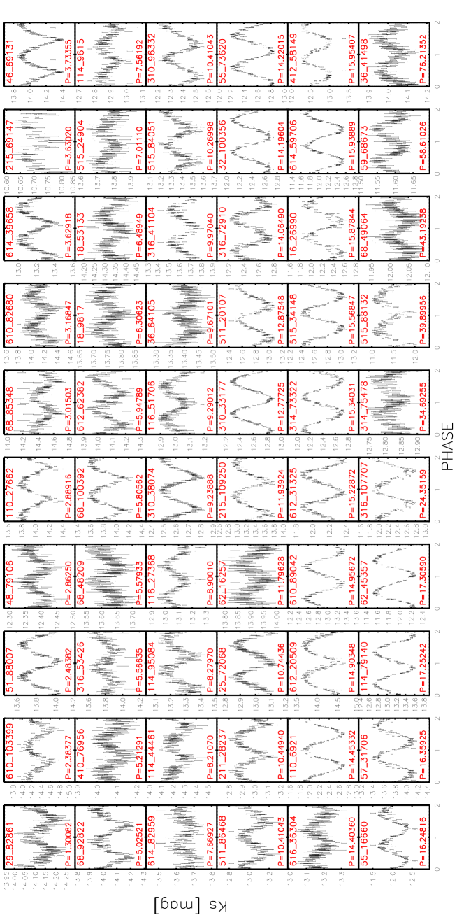
Figure 6: Phased $K_{s}$-band light curves of 60 variable stars classified as T2Cs. Periods are labeled at the bottom of each panel. The “b333” part of the name is omitted.

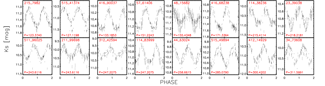
Figure 7: As in Fig. 6 but for the 16 variable stars in common with the sample of M09. We note that, while all of these were classified as Miras by M09, our classification does not always match. For a more detailed discussion, see Section 5.4.

5 Matches with other catalogs

Although this work presents the most extensive survey of this region of the Galaxy for variables with periods longer than one day, and despite most of our targets being new detections, some were already found in similar investigations. In the following paragraphs, we compare our list with those found previously in the literature, more specifically, within the VSX catalog, the OGLE survey and—in order of increasing variable period (from RRLs, T2Cs, CCs to Miras)—CR18, M13, and M09. We did not find any match with the variables found by Dong et al. (2017) within the nuclear star cluster.

5.1 VSX and OGLE catalogs

We crossmatched our list of candidate variables with those in the VSX catalog and those found by the OGLE survey to see whether or not some of our variable candidates had already been found and/or classified. Indeed, we found nine matches within the eclipsing binaries catalog of the OGLE IV survey (Soszyński et al. 2016) and 77 matches in the VSX catalog. The literature names of these matching variables are displayed in the second column of Table 2.

The crossmatches were performed by selecting a conservative radius for the cone search of 3 arcsec. The VSX matches were all found within 2.4 arcsec, while the OGLE matches are within 1.4 arcsec from our own position. We checked that the quoted matches are indeed the same objects that were found in our investigation by comparing not only the distance from our position, but also the magnitude and, when needed, the finding charts. The matching sources in the VSX catalog were originally detected by Wood et al. (1998), Glass et al. (2001); M09, Matsunaga et al. (2011) and M13. More precisely, we find 15 sources in common with Wood et al. (1998), 2 in common with Glass et al. (2001) , and the remaining 60 are the CCs by Matsunaga et al. (2011), the 16 T2Cs by M13, 7 eclipsing/unknown type variables by M13, and 34 LPVs by M09. Curiously, only 4 bona fide Miras by M09 were retrieved in the VSX catalog, although we found 16 common variables by directly matching our catalog to the catalog of bona fide Miras of M09 (see Section 5.4). By summing up all this information, we conclude that the variables that were already known before this work are 77 VSXs, 9 OGLE EBs, 12 M09 Miras (not retrieved within the VSX), and 3 RRLs (Contreras Ramos et al. 2018, see Section 5.2), making a total of 101.

We conclude this section by pointing out that our independent classification accurately matches those in the literature. In fact, the candidate variables matching the catalogs of Wood et al. (1998) and Glass et al. (2001) were all classified as either OH stars or Miras; our classification for these stars is either “Mira” or “Mira?”, thus matching the classification provided by the quoted studies. Concerning the matches with variables in the M09, Matsunaga et al. (2011), and M13 series of studies, more details are provided in Sects. 5.3 and  5.4.

5.2 RR Lyr catalog of CR18

As discussed in Section 3.3.1, our periodicity search algorithm focused on periods longer than 1 day, and the variables with shorter periods are an incomplete sample. Nonetheless, our final catalog contains some candidate RRLs that are either uncertain or bona fide. We matched our catalog with the list of RRLs published by CR18 and found three sources in common. We note that we performed the match by ID because we used the same photometric data set. This means that there is no uncertainty associated to a cone search by coordinates.

The common sources are b333_616_55278, b333_614_37068 and b333_414_55144, which we classified as RRab/NPV/ACFU, RRab/ACFU, and RRab, respectively. Also, we note that in our catalog, we found four RRabs that were not detected by CR18 (b333_201_84779, b333_304_81788, b333_201_45267 and b333_201_65407).

5.3 T2C and CC catalog of M13

A previous search for Cepheids towards the Galactic center was performed by M13 with the NIR SIRIUS camera at the IRSF 1.4m telescope. They found 45 variable stars, of which 20 were classified as Cepheids (16 T2Cs, 3 CCs and one generic Cepheid candidate).

The b333 tile overlaps completely with the IRSF survey sky area and we retrieved all the 20 Cepheids by M13 within our initial list of $\sim$5 million sources. However, our periodicity search algorithm detected only 14 of them. Six Cepheids were not retrieved because their light curves have many uncertain phase points due to either saturation and/or blending. We manually extracted the light curves of the six missing Cepheids and, by knowing a priori their periods, we manually rejected the poor-quality data and obtained clean light curves for five of them. Unfortunately, b333_114_65025 is affected by severe blending and it was not possible to detect any periodic behavior even knowing the period a priori. We note that M13 also pointed out that this star (their #2) is in a very crowded field and that their photometry was not accurate.

The comparison with the M13 sample also provides a validation of our classification criteria. In fact, among the 14 variables that were retrieved automatically, we classified – without knowing, a priori, the classification by M13 – 13 of them as T2Cs and one as “T2C?”. We then checked the two samples and found that our classifications match those of M13, including their “Cep(?)”, which is our “T2C?”.

We provide a more detailed discussion of the offsets in distance and reddening between our estimates and those of M13 in Section 5.5.

5.4 Miras catalogs of M09

Using the NIR SIRIUS camera at the IRSF 1.4m telescope, M09 found 175 Miras towards the GC, and estimated their periods, distance, and extinction. They performed a sample selection based on the period, and marked only those with periods between 100 and 350 days as bona fide Miras, since they are the least affected by circumstellar reddening. We found a matching source for all their Miras in our initial photometric catalog. However, only 16 of them were retrieved in our final catalog of variable candidates. The reason for the low fraction of Miras retrieved in our final catalog is that M13 Miras are mostly located in the Bulge, therefore they are saturated – more severely than T2Cs – or are in the nonlinear regime of the VISTA images. A more complete discussion of these and other Mira variables in the VVV data will be presented in Nikzat et al. (2019, in preparation).

Of these 16 variable candidates, 9 were classified as Miras, 6 as “Mira?”, and one as an SRV. We point out that the offset in mean magnitude between our catalog and that of M13 is small: the mean offset is 0.002$\pm$0.092 mag, although for one variable (b333_416_5350, M09 #1043) the offset is as large as 0.218 magnitudes brighter in M13. However, the offsets on $Amp(K_{s})$ are larger. As a matter of fact, for nine among the 16 variables, the offset in $Amp(K_{s})$ is larger than 0.1 mag, and for two of them it is as large as $\Delta A_{Ks}\sim$2.0 mag, which has dramatic effects on the distance estimates. We found that $\Delta Amp(K_{s})$ is not correlated with the mean magnitude.

We provide a more detailed discussion of the offsets in distance and reddening between our estimates and those of M09 in Section 5.5.

5.5 A caveat on extinction and distance

In principle, the offsets in distance are not to be fully ascribed to offsets in reddening. As mentioned in Section 3.1, IRSF and VISTA have different diameters (1.4m vs 4m). This means that stars in the linear photon count regime of the SIRIUS camera on IRSF can be saturated in VIRCAM. Figure 8 displays the difference in mean magnitude for the common sources.

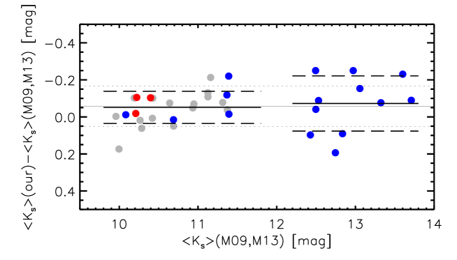
Figure 8: Mean magnitude offset between our magnitudes and those by M09 and M13 ($\langle K_{s}\rangle(M09,M13)$). Blue circles display T2Cs, red circles display CCs, and gray circles display Miras. The black solid line represents the average, and the black short-dashed lines the standard deviation of the whole sample. The black, thick, solid, and long-dashed lines have the same meaning for saturated ($\langle K_{s}\rangle<$12 mag) and nonsaturated ($\langle K_{s}\rangle>$12 mag) targets in the VVV.

Within the dispersion, which is very large ($\sim$0.1 mag), the average is zero. However, somewhat surprisingly, both the offset and the dispersion are larger for nonsaturated VVV targets than for saturated targets. The large individual offsets might be due to the different pixel scales of the two cameras: 0.25 mas/pix for VIRCAM and 0.45 mas/pix for SIRIUS. In such a crowded region, VIRCAM has the advantage of a spatial resolution that is almost twice as great as that of SIRIUS, meaning that it is more capable of resolving neighboring stars. Overall, we can conclude that the different saturation levels and pixel scales do not significantly affect the mean magnitudes, but the effect on individual stars is large, up to $\pm$0.2 mag, meaning a relative systematic offset of up to $\sim$8% on the distance.

Once it had been found that the offsets in $K_{s}$ have a minor impact on distances, we inspected the effects of the offsets in extinction. As mentioned in Section 4, for targets like CCs and T2Cs, we derived two sets of distance and extinction. We compare the $A_{Ks(PL)}$ and $d_{PL}$ with those from M09 and M13. The main difference is that they used the Nishiyama et al. (2006, 2009) reddening law, which provides a different $\dfrac{A_{Ks}}{E(J-K_{s})}$ ratio from ours (0.499 versus the 0.428 average value in Alonso-García et al. 2017). This means that for a homogeneous comparison we need to compare $E(J-K_{s})$ and not $A_{Ks}$.

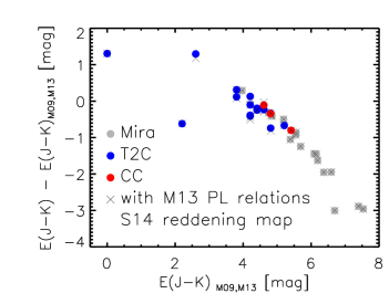
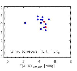
Figure 9: Left: Offset between our reddening $E(J-K_{s})$—obtained with the S14 reddening map—and that by M09 and M13 ($E(J-K_{s})_{M09,M13}$) vs. $E(J-K_{s})_{M09,M13}$ for the common targets. The symbols are the same as those in Fig. 8. The black crosses mark the same information, but using the same calibrating PLs as M13. Right: As in the left panel but for our $E(J-K_{s})$ derived using the PL$HK_{s}$ solution.

For a rigorous interpretation of Fig. 9 one should take into account that in Section 4 we have adopted the same PL$K_{s}$ used by M09 for Miras, but different PL relations for T2Cs and CCs. Therefore, Fig. 9 also shows our $E(J-K_{s})$ estimates both using the PLs listed in Table 1 (circles in Fig. 9) and using the same relations as M09 and M13, converted to the VISTA photometric system (crosses in Fig. 9). We note that to adopt the different calibrations of the PLs does not qualitatively change the observed trends. Furthermore, using the S14 map (left panel), our $E(J-K_{s})$ estimates are always smaller than 5 mag, while those by M09 and M13 can be as large as $\sim$7.5 mag and $\sim$5.5 mag, respectively. These offsets generate the displayed trend: using the PL$HK_{s}$ solution for distance and $A_{Ks}$, the trend does not show up and the average offset is zero, within the standard deviation. Unfortunately, not all the common targets have a photometric PSF solution in our $H$ band images, since they are extremely faint, and therefore the sample is smaller. The fraction of targets with a PSF solution in the $J$ band drops dramatically, and it is pointless to perform the same analysis on them. We remind the reader that we did not adopt this technique for Miras (see Section 4, point 3c).

Most probably, the resolution of the S14 reddening map ($6\times 6$ arcmin) is insufficient to reproduce the fine details of the reddening patterns towards the GC, and the average values seem to be, overall, underestimated. One might expect that adopting the G12 reddening map, which has a resolution of 2 arcmin, would diminish this effect, but the average offset is negligible and the individual distances are even less reliable. In fact, using the G12 map, T2Cs display a very unlikely double-peaked distance distribution.

These offsets in reddening translate into significant distance offsets, which become dramatic for Miras, as displayed in Fig. 10.

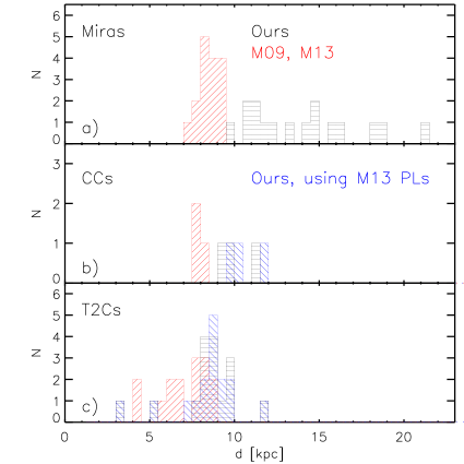
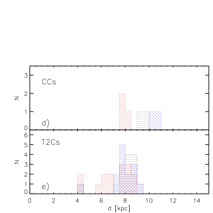
Figure 10: Panel a): Distance distribution of Miras. Red: M09 distances, Black: our distances. Panel b): as in panel (a) but for CCs. Blue bars mark the distances derived adopting the same PL as M13. Panel c): as in panel (b) but for T2Cs. Panel d): as in panel (b) but using the distances estimated with the PL$HK_{s}$ relations. Panel e): as in panel (c) but using the distances estimated with the PL$HK_{s}$ relations.

Miras — The difference in reddening—and, in turn, on distances—is, on average, larger for Miras than for T2Cs and CCs. M09 estimated the distances to these targets to be smaller than 10 kpc for all of them. Most of them are located at between 7 and 10 kpc, and their peak is around 8.5 kpc, indicating that they belong to the Bulge. On the other hand, our distances are all larger than 10 kpc and their spatial distribution is almost constant over the 10-25 kpc distance range. One might invoke circumstellar extinction – which is accounted for in M09 extinction estimates, but not in the S14 map – to justify these offsets. However, as already mentioned, Miras with such short periods ($<$350 days) should not be significantly affected by circumstellar extinction (Ita & Matsunaga 2011). This means that, while possibly present, circumstellar extinction cannot, by itself, account for the whole offset. As mentioned above, we did not adopt the PL$HK_{s}$ solution for Miras.

CCs — These three Cepheids were first found by Matsunaga et al. (2011), who claimed that they are Bulge stars, and the first CCs ever found close to the GC. However, our different extinctions provide larger distances, which put them on the other side of the thin disk, at more than 9 kpc, both for $d_{S14}$ and $d_{PL}$, with small differences ($\lesssim$0.4 kpc) between the two distance sets. We point out that, although these targets are saturated in the VVV, the difference between our $\langle K_{s}\rangle$ and those by M13 are small (–0.056 mag, 0.021 mag and –0.063 mag, for b333_215_87770, b333_215_86376 and b333_515_65036, respectively, where negative values indicate brighter $\langle K_{s}\rangle$ in our catalog). This means that the distance offsets displayed in the middle panel of Fig. 10 are not caused by a poor estimate of their mean magnitude, but should be ascribed to the difference in extinction only. We note that the adoption of the same PL as M13 affects the distances at a level of $\lesssim$0.3 kpc for the $d_{S14}$ sample – which is negligible compared to our errors – and $\sim$1 kpc for $d_{PL}$.

T2Cs — For all but three targets, we obtain a $d_{S14}$ that is larger by 1-2 kpc with respect to M13 distances, although a few objects show distances that are similar or smaller (b333_215_69147, which is M13 #19; b333_416_9672, which is M13 #34; b333_515_84051, which is M13 #29). On the other hand, $d_{PL}$ are on average the same as those obtained by M13.

To sum up, the effect on the distance estimates of the offsets in $A_{Ks}$ is on average that of shifting targets to higher distances. However, at least for T2Cs, using the PL$HK_{s}$ method provides results that are similar to those of M13. Since most of these targets are saturated, their proper motions have large uncertainties, and therefore we could not decipher which set of $A_{Ks}$-distances is correct based on their proper motions (e.g., the three CCs should have disk kinematics if our distance estimates are correct).

Therefore, we inspect the $d_{S14}$ and $d_{PL}$ distribution of T2Cs in greater detail; they are displayed as light blue histograms in Fig. 13. The plain distributions provide biased information. In fact, one must take into account the depth effect, which makes farther stars more likely to be detected. In fact, the number of stars detected increases quadratically with distance, because larger volumes are surveyed at larger distances. To take this geometric effect into account, we scaled the distributions by $d^{-2}$. We fitted the rescaled distributions (blue histograms in Figure 11) with Gaussians.

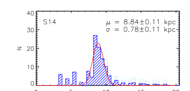
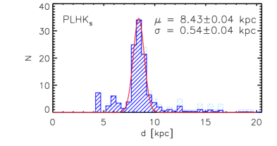
Figure 11: Top: Light blue dashed histogram showing the $d_{S14}$ distribution of BLHs and WVs within 20 kpc. The dark blue histogram shows the rescaled distance distribution (see text). The red solid line shows a Gaussian fit to the rescaled distribution. The abscissa of the peak and the sigma of the Gaussian are labeled. Bottom: As in top, but for $d_{PL}$.

The peaks of the Gaussians of $d_{S14}$ and $d_{PL}$ are 8.84$\pm$0.11 kpc and 8.43$\pm$0.04 kpc, respectively. This technique is usually adopted to estimate the distance of the GC (Groenewegen et al. 2008; Dékány et al. 2013; Pietrukowicz et al. 2015; Bhardwaj et al. 2017b; Contreras Ramos et al. 2018; Braga et al. 2018a) but our result using the S14 map is relatively large compared to the recommended value of 8.3$\pm$0.2(stat.)$\pm$0.4(syst.) kpc (de Grijs & Bono 2016) and compared to the new geometric estimate of the distance of Sgr A* with GRAVITY (8.127 kpc; Gravity Collaboration et al. 2018). Moreover, the bin enclosing distances between 7.5 and 8.0 kpc is undersampled in $d_{S14}$, making the distribution fairly asymmetrical. This is further evidence that the S14 map does not provide extinctions that are systematically offset by a fixed amount, but rather shows that there are individual offsets in $A_{Ks}$. On the other hand, the distances obtained using the PL$HK_{s}$ method are more reliable, because the peak of Gaussian is closer to the estimates in the literature. Finally, the smaller HWHM of the $d_{PL}$ distribution goes in the correct direction. In fact, although investigations of the spatial distrubution of RRLs and T2Cs towards the entire Bulge generally provide larger HWHM ($\sim$0.8-1.0 kpc Pietrukowicz et al. 2015; Bhardwaj et al. 2017b), our investigation is more limited in sky area, and therefore we expect a tighter distribution of T2Cs.

Finally, we discuss the huge effect played by the reddening law. Not only, as already mentioned, is the total-to-selective absorption ratio $\dfrac{A_{Ks}}{E(J-K_{s})}$ different between Nishiyama et al. (2006, 2009) and Alonso-García et al. (2017), but a macroscopic effect is played by the extinction ratio $A_{H}/A_{Ks}$, which is 1.731 and 1.88 for the two reddening laws, respectively. Of course the photometric systems are different, and therefore the comparison is not straightforward. Nonetheless, the PL$HK_{s}$ method strongly depends on this ratio and the effect is a systematic decrease of the distances by $\sim$1.2 kpc when using the Nishiyama et al. (2006, 2009) reddening law.

All of these considerations provide strong evidence that further insight into the reddening law towards the central-most regions of the Galaxy is needed in order to correctly interpret the results of past and future observations, especially due to the uncertainty on distances and differential reddening effects.

6 Catalog properties

The positions of the 1,019 PVSs in the Galaxy are displayed in Fig. 12. The T2Cs (blue diamonds) are uniformly distributed within the b333 tile. This is expected, since T2Cs are mostly old, with a fraction of intermediate-age stars (Wallerstein 2002; Iwanek et al. 2018).

We also point out that the position of RRLs, which are found only close to the borders of the tile, is due to the intrinsic faintness of these objects. This is consistent with the spatial distribution of RRLs found by CR18, that is, they are located around the GC but their sky surface density decreases towards the GC itself (see their Figure 6).

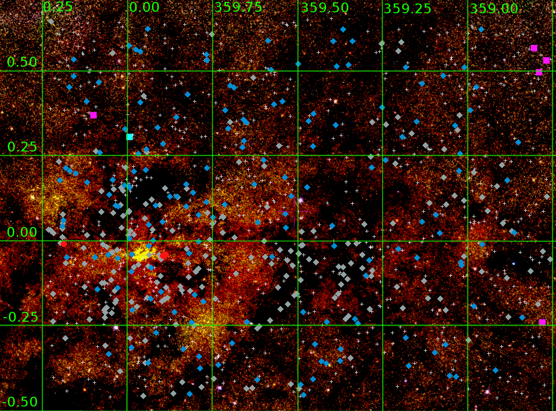
Figure 12: Map in Galactic longitude and latitude ($l$,$b$) showing the distribution in the sky of the sample variable stars. Map obtained with Aladin Sky Atlas v10.076 (Bonnarel et al. 2000), using the 2MASS $JHK_{s}$ images catalog (Skrutskie et al. 2006). Blue diamonds represent T2Cs, which are spread over the whole field. Gray diamonds display Miras, which are more concentrated at low latitudes. Red ovals display CCs (the ones by Matsunaga et al. 2011). The magenta squares in this map are the RRLs, the cyan square is the AC, and the small white plus symbols represent all the other types of variables.

The distribution of the periods of our variables, displayed in Fig. 13, outlines some interesting features. First of all, we note a lack of variables in the interval between $\sim$20 and $\sim$365 days. The reason for this lack of stars is due to the aliases at one year and at half a year, and to the transition between WVs and RVTs: the light curves of RVTs might display alternating deep and shallow minima, and are therefore more difficult to classify.

Six of the nineteen RVTs display clear alternating minima. We have inspected their position and conclude that they are not peculiar with respect to the other RVTs and T2Cs in general. (Soszyński et al. 2017) found that WVs with periods longer than 16 days also might show alternating minima, but we did not find any of these.

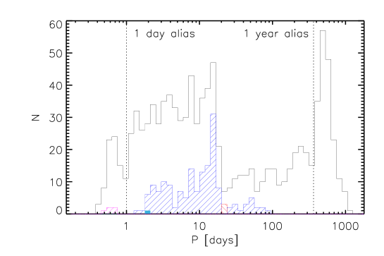
Figure 13: Period distribution of our final list of PVSs. The dashed lines mark the aliases at 1 day and 1 year. The black histogram includes all the 1,019 candidate PVSs found, the dashed magenta, blue, and red histograms represent RRabs, T2Cs, and CCFUs, respectively. The filled light blue bin at P$\lesssim$2 days represents the ACFU.

Figure 13 also displays a lack of variables with solid classification in the period between 1 and 2 days, despite the large number of variables (119) detected at these periods. This is mainly due to the overlap of many variable types (T2Cs, CCFOs, CCFUs, ACFOs, ACFUs) in that region of the Bailey diagram, which is one of our main diagnostics for the classification. This lack of variables with unambiguous classification in this period range is even more clear in the Bailey diagram (Fig. 14).

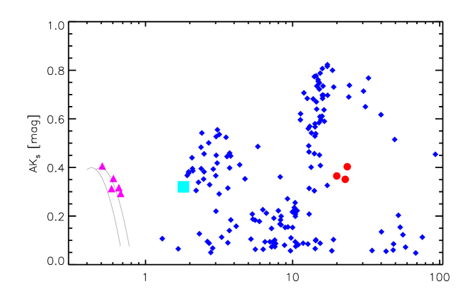
Figure 14: Bailey diagram of the PVS in our final list. Small black plus symbols mark the position of stars with uncertain classification. Blue diamonds mark T2Cs, magenta triangles mark RRab stars, red circles mark CCFUs, and the cyan square marks the ACFU. The solid lines represent the Oosterhoff I (left) and Oosterhoff II (right) sequences of RRab stars (Cacciari et al. 2005), rescaled using $Amp(K_{s})/AB$ amplitude ratios (Braga et al. 2018c).

Figure 14 also shows that the T2Cs follow the usual double-peaked period distribution (Catelan & Smith 2015, and references therein). It also shows that we detected variables with $Amp(K_{s})$ as small as 0.047$\pm$0.016 mag, thanks to the loose constraints described in Section 3.1. The five RRabs, on the other hand, follow the Oosterhoff II sequence. For the definition of the Oosterhoff groups, the reader is referred to Oosterhoff (1939); Catelan & Smith (2015). This is surprising, given the fact that the Oosterhoff classification is an indicator of metallicity (Kinman 1959), and Oosterhoff II RRLs should be the most metal-poor. In fact, Kunder & Chaboyer (2009) and Contreras Ramos et al. (2018), among others, found that bulge RRLs are much more likely to belong to the Oosterhoff I population. This result does not change when adopting the amplitude ratio by Navarrete et al. (2015).

The observed CMD (left panel in Fig. 15) clearly shows the effects of large differential reddening in the field. In particular, a substantial fraction of the stars is displaced along the reddening vector (red arrow).

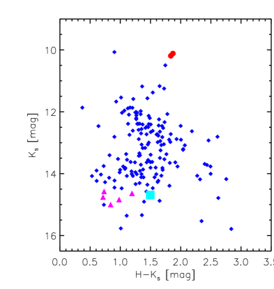
Figure 15: $\langle K_{s}\rangle$ vs. $H-\langle K_{s}\rangle$ CMD of the candidate variable stars in our sample. The symbols are the same as in Fig. 14. The red arrow displays the reddening vector in arbitrary units.

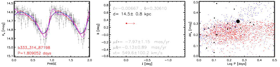
Figure 16: Left: $K_{s}$-band Light curve of the ACFU star b333_314_87198. The name and period are labeled. The magenta line is the fourth-order Fourier fit. Blue and red lines are the template fits of T2Cs and CCs, respectively, in this period range. Middle: Position and proper motion of the target. Galactic coordinates, distance, proper motion in galactic coordinates, and tangential velocity are labeled. We note that the arrow and the tangential velocity were derived by summing the proper motion of Sgr A* to our own proper motions. Right: The large black circle represents the target in the Bailey (amplitude vs. period) diagram. The position of both Milky Way, LMC, and SMC ACs, T2Cs and CCs are marked in black, blue, and red, respectively.

One unexpected result is the detection of the first AC in this sky area (b333_314_87198, see Fig. 16). This star has a period of 1.80905 days, which, as already mentioned, is within the range of many types of variables. However, its position in the Bailey diagram (see right panel of Fig. 16) restricts the possible classification to ACFU, T2C, and CCFU only, the latter being very unlikely (see discussion on its tangential velocity below). However, it is the peculiar shape of its low-noise light curve—with an extremely steep rising branch—which leaves no doubt on its classification. At these periods, T2Cs and CCFU stars have more shallow light curves (Inno et al. 2015; Bhardwaj et al. 2017a). According to our estimates, its distance is 14.4$\pm$0.7 kpc. Also taking into account systematic uncertainties due to reddening, there is no way that this ACFU can be within the Bulge. We derived a height above the Galactic plane of only 83$\pm$4 pc. Moreover, its proper motion has an almost null latitudinal component (Fig. 16, middle panel). However, its tangential velocity is too small (109.2$\pm$99.4 km/s) to be consistent with thin disk dynamics, and therefore it must be either a halo or a thick disk star. Spectroscopic follow-ups of the target are planned to constrain its chemical and dynamical properties. We have already submitted a proposal for observations with FIRE@Magellan. These will be useful to better constrain the complicated evolutionary picture of ACs, which is, to date, uncertain (Fiorentino & Monelli 2012; Iwanek et al. 2018).

7 Conclusions

We present the most extensive catalog of variable stars in the region of the GC, which includes 1,019 objects. The catalog contains accurate coordinates, NIR ($ZYJH$) magnitudes, $K_{s}$-band mean magnitudes, $K_{s}$-band light amplitudes, and periods. We also provide proper motions for 530 targets and extinctions $A_{Ks}$ plus individual distances for 220 targets. For 472 variables, we provide a high-rank, unambiguous classification. The latter sample includes 5 RRab, 164 T2Cs, 3 CCFU, 1 ACFU, 16 SRVs, 210 Miras, and 73 NPVs (of which 47 DEBs).

For all these candidate variables, we show the NIR CMDs, proper motions, period distributions, and spatial distributions for the different types of variable stars, including important distance indicators (RRLs, Cepheids).

T2Cs — 164 bona fide T2Cs, among which 45 BLHs, 100 WVs, and 19 RVTs were retrieved. Type II Cepheids are uniformly distributed across the b333 field of view. It was not trivial to provide a solid classification for variables with periods between 1 and 2 days because in that period range many possible types of variability overlap (T2Cs, CCFUs, CCFOs, ACFUs, ACFOs, and all types of eclipsing binaries). We have looked in detail into their individual reddening estimates—both individual and using extinction maps—and we investigated their distance distribution. We also compared our results with those by Matsunaga et al. (2013) since there are 16 T2Cs in common, but all we can conclude is that our distances are 1-2 kpc larger than those found in the literature. This is a very large offset, but this should not be surprising. In fact, we estimate that a $\sim$10% offset in the $A_{H}/A_{Ks}$ extinction ratio causes a shift as large as $\sim$1.2 kpc in the estimate for a star at the distance of the GC, using the same calibrating relations, $E(J-K_{s})$, mean magnitudes, and photometric system. This is a stark warning for all works focusing on distance estimates in regions that are close to the GC.

Miras — We retrieved 210 Miras candidates with periods between 87 and 943 days. We did not publish their astrophysical properties (coordinates, periods, mean magnitudes, etc.) because this is the aim of Nikzat et al. (2019). Nonetheless, we compared our photometric solution with that of Matsunaga et al. (2009). The effect of the uncertainties on reddening are dramatic for short-period ($P<350$ days) Miras and turn into differences in distance as large as 10 kpc. Invoking circumstellar extinction is not enough to justify these differences, and both the amount of reddening and the difference in the adopted reddening law (Nishiyama et al. 2009 and Alonso-García et al. 2017) play a major role in contributing to systematic uncertainties.

CCs — Among the point-source catalog of our PSF photometry, we retrieved the three CCs found by Matsunaga et al. (2011). However, our periodicity search algorithm did not automatically detect them, since their light curves are relatively noisy. By adopting an a priori period, we were able to remove outliers from the light curves and fit their light curves to derive mean magnitudes and amplitudes.

ACFU b333_314_87198 — We found the first AC in this sky area. There is evidence that this star pulsates in the Fundamental mode and that it is located on the other side of the Bulge. However, despite its proper motion having an almost null latitudinal component, its velocity is not consistent with thin-disk dynamics, and therefore it must be either a halo or a thick disk star.

The published catalog is a starting point for any detailed investigation of variable stars within the inner Galactic Bulge. As a matter of fact, to exploit the potentialities of variable stars as extinction and distance indicators, only a multi-band (NIR and, eventually, mid-infrared) and combined photometric and spectroscopic investigation will allow for the systematic uncertainties to be lowered. For this reason, we are planning to submit NIR spectroscopic follow-ups of these targets to better constrain their physical properties. This catalog also provides targets for future NIR spectroscopic surveys (SDSS-V, 4MOST) and deep optical photometric surveys like the Large Synoptic Survey Telescope (LSST, Ivezic et al. 2009), and NIR photometric surveys like the Wide Field Infrared Space Telescope (WFIRST, Spergel et al. 2015).

Acknowledgments: We gratefully acknowledge data from the ESO Public Survey program ID 179.B-2002 taken with the VISTA telescope, and products from the Cambridge Astronomical Survey Unit (CASU). Support is provided by the Ministry for the Economy, Development and Tourism, Programa Iniciativa Cientifica Milenio grant IC120009, awarded to the Millennium Institute of Astrophysics (MAS), and by the BASAL Center for Astrophysics and Associated Technologies (CATA) through grant AFB-170002. D.M. acknowledges support from FONDECYT Regular grant No. 1170121. M.C. and F.N, acknowledge additional support from FONDECYT regular grant No. 1171273 and CONYCYT’s PCI grant No. DPI20140066. This research has made use of “Aladin sky atlas” developed at CDS, Strasbourg Observatory, France

References

- Alonso-García et al. (2017) Alonso-García, J., Minniti, D., Catelan, M., et al. 2017, ApJ, 849, L13
- Anderson et al. (2016) Anderson, R. I., Saio, H., Ekström, S., Georgy, C., & Meynet, G. 2016, A&A, 591, A8
- Bhardwaj et al. (2015) Bhardwaj, A., Kanbur, S. M., Singh, H. P., Macri, L. M., & Ngeow, C.-C. 2015, MNRAS, 447, 3342
- Bhardwaj et al. (2017a) Bhardwaj, A., Macri, L. M., Rejkuba, M., et al. 2017a, AJ, 153, 154
- Bhardwaj et al. (2017b) Bhardwaj, A., Rejkuba, M., Minniti, D., et al. 2017b, A&A, 605, A100
- Bica et al. (2018) Bica, E., Minniti, D., Bonatto, C., & Hempel, M. 2018, PASA, 35, e025
- Bonnarel et al. (2000) Bonnarel, F., Fernique, P., Bienaymé, O., et al. 2000, A&AS, 143, 33
- Bono et al. (2001) Bono, G., Caputo, F., Castellani, V., Marconi, M., & Storm, J. 2001, MNRAS, 326, 1183
- Bono et al. (2000) Bono, G., Castellani, V., & Marconi, M. 2000, ApJ, 529, 293
- Bono et al. (2005) Bono, G., Marconi, M., Cassisi, S., et al. 2005, ApJ, 621, 966
- Braga et al. (2018a) Braga, V. F., Bhardwaj, A., Contreras Ramos, R., et al. 2018a, A&A, 619, A51
- Braga et al. (2018b) Braga, V. F., Stetson, P. B., Bono, G., et al. 2018b, arXiv e-prints [arXiv:1812.06372]
- Braga et al. (2018c) Braga, V. F., Stetson, P. B., Bono, G., et al. 2018c, AJ, 155, 137
- Cacciari et al. (2005) Cacciari, C., Corwin, T. M., & Carney, B. W. 2005, AJ, 129, 267
- Catchpole et al. (2016) Catchpole, R. M., Whitelock, P. A., Feast, M. W., et al. 2016, MNRAS, 455, 2216
- Catelan et al. (2004) Catelan, M., Pritzl, B. J., & Smith, H. A. 2004, ApJS, 154, 633
- Catelan & Smith (2015) Catelan, M. & Smith, H. A. 2015, Pulsating Stars
- Contreras Ramos et al. (2018) Contreras Ramos, R., Minniti, D., Gran, F., et al. 2018, ApJ, 863, 79 [CR18]
- Contreras Ramos et al. (2017) Contreras Ramos, R., Zoccali, M., Rojas, F., et al. 2017, A&A, 608, A140
- de Grijs & Bono (2016) de Grijs, R. & Bono, G. 2016, ApJS, 227, 5
- Dékány et al. (2013) Dékány, I., Minniti, D., Catelan, M., et al. 2013, ApJ, 776, L19
- Di Criscienzo et al. (2007) Di Criscienzo, M., Caputo, F., Marconi, M., & Cassisi, S. 2007, A&A, 471, 893
- Dong et al. (2017) Dong, H., Schödel, R., Williams, B. F., et al. 2017, MNRAS, 471, 3617
- Feast et al. (2008) Feast, M. W., Laney, C. D., Kinman, T. D., van Leeuwen, F., & Whitelock, P. A. 2008, MNRAS, 386, 2115