Discovering Common Change-Point Patterns in Functional Connectivity Across Subjects

Abstract

This paper studies change-points in human brain functional connectivity (FC) and seeks patterns that are common across multiple subjects under identical external stimulus. FC relates to the similarity of fMRI responses across different brain regions when the brain is simply resting or performing a task. While the dynamic nature of FC is well accepted, this paper develops a formal statistical test for finding change-points in times series associated with FC. It represents short-term connectivity by a symmetric positive-definite matrix, and uses a Riemannian metric on this space to develop a graphical method for detecting change-points in a time series of such matrices. It also provides a graphical representation of estimated FC for stationary subintervals in between the detected change-points. Furthermore, it uses a temporal alignment of the test statistic, viewed as a real-valued function over time, to remove inter-subject variability and to discover common change-point patterns across subjects. This method is illustrated using data from Human Connectome Project (HCP) database for multiple subjects and tasks.

1 Introduction

Learning about structural and functional connectivity in human brain is of great interest from many perspectives. The recent Human Connectome Project (HCP) investigates these connectivities in order to understand brain functionality and its relation to the cognitive abilities of individual subjects. Functional connectivity (FC) is observed using functional MRI (fMRI) data and is believed to capture interactions between brain regions with or without external stimuli. It is different from structural connectivity which describes anatomical links between brain regions and is estimated using structural MRI or diffusion MRI. FC is defined as a set of statistical dependencies among remote anatomical regions due to neurophysiological events (Friston (2011)). These dependencies are expressed as quantifications of similarity, or correlations, between simultaneous functional measurements of neuronal activities across regions in the human brain. Functional MRI measures the blood oxygen level dependent (BOLD) contrast signals of each brain voxel over a period of time. The short-term FC is often represented as a covariance or correlation matrix of fMRI data over a small time window, with the matrix size equal to the number of brain regions being considered. In the early days, FC associated with individual tasks or stimuli was treated as fixed or static over observation time. However, recent studies (Hutchison et al. (2013); Monti et al. (2014); Hindriks et al. (2016)) have revealed strong evidence that FC is a dynamic process and evolves over time, even in the resting state. Our primary interest is to investigate and characterize the dynamic nature of FC between different anatomical regions during performances of certain tasks and in resting states. A dynamic FC model is bound to provide broader insight into fundamental mechanism of brain networks (Lindquist et al. (2014)). For a review on recent progress in analyzing FC, please refer to Friston (2011); Hutchison et al. (2013).

A critical part in modeling dynamic FC is to quantify changes that occur over time during observation intervals. For example, some studies have developed tests for temporal changes in coherence pattern of multiple regions of interest (ROIs) Poldrack (2007). Cribben et al. (2012) introduced Dynamic Connectivity Regression (DCR), which is a data-driven technique for detecting temporal change points in functional connectivity between brain regions. Later on, Cribben et al. (2013) presented a modified DCR on single-subject data that increases accuracy with a small number of observations and reduces the number of false positives. In case FC is represented by a covariance or a correlation matrix of fMRI signals, a sliding (time) window is commonly used to estimate the dynamic FC as a time series of such matrices. Lindquist et al. (2014) discuss some alternatives to moving window-based correlation estimation. Xu and Lindquist (2015) have proposed an advancement of DCR into a dynamic connectivity detection algorithm that uses statistical models at node level and can handle much larger number of regions than DCR. More recently, Barnett and Onnela (2016) proposed a method for detecting change-points in correlation networks that requires minimal distributional assumptions. Jeong et al. (2016) presented a semiparametric mixture model which is less sensitive to the window size selection in detecting change-points in large-size functional networks of resting-state fMRI. Xiao et al. (2017) studied the problem of change-point detection based on Bayesian inference and genetic algorithms.

While several of these studies focus on testing whether FC is static or dynamic, or seek temporal change-points for individual subjects, we additionally analyze FC in a group of individuals and seek some common patterns of FC during performances of identical tasks. We take different partitionings of human brain into functional units or regions of interests (ROIs) and represent short-term FC as symmetric, positive definite matrices (SPDMs), with entries denoting covariances of localized BOLD signals. We use a sliding window technique to segment multivariate time series into overlapping blocks, and compute a covariance matrix for each block. The original time series data can thus be converted into a time-indexed sequence of SPDMs and one of the goals is now to detect if these sequences denote a stationary process or if the underlying probability distribution switches at one or multiple time points. The actual test is performed using a nonparametric graphical approach, introduced in Chen and Zhang (2015), that uses minimal spanning trees (MSTs) connecting the observed SPDMs in a certain metric space. Even though this approach is derived for $i.i.d.$ samples, we empirically demonstrate that it is also effective in case of dependent time series data. We utilize a Riemannian structure of the space of SPDMs to define and compute geodesic distances between covariance matrices, and to facilitate the construction of MSTs. Computation of edge length distributions across temporal partitions of nodes in MSTs lead to a test statistic for change-point detection. The final algorithm depends on a number of parameter choices for forming and testing covariance trajectories. While the proposed method is naturally dependent on the choices of these parameters, we demonstrate that the results are relatively stable with respect to these choices as long as they are in a reasonable range as dictated by the experimental setting.

The change-point patterns for a group of people are expected to be similar, especially when the fMRI data are recorded in a well-designed experiment where tasks are sequentially performed at pre-determined time blocks. However, different subjects may react differently to external stimuli and the response times can be different. Additionally, data variability and algorithmic imprecision add to the variability in the detection results. Thus, it is naturally difficult to discern the commonality of change-point patterns across subjects from the raw change-point inferences. One solution to reducing inter-subject variability in the time domain is to perform temporal alignment, to allow discoveries of underlying patterns. We apply temporal alignment at the level of test statistics to detect and discover some common patterns of FC dynamics for a group of individuals. We further validate these patterns by comparing them with block designs governing the task-related external stimuli using the HCP data. The proposed methodology is also comprehensively tested with simulated data and validated by comparisons with the ground truth. The novel contributions of this paper are as follows:

1. It introduces an end-to-end pipeline for change-point detection in individual subject data, starting from raw fMRI data all the way to detected change-points in FC.

2. It represents short-term connectivity using covariance matrices and long-term data as covariance trajectories, and utilizes the Riemannian geometry of SPDM space for developing test statistics.

3. It adapts the graph-based change-point detection algorithm presented in Chen and Zhang (2015) to this problem area, and demonstrates the feasibility of this solution on a large set of real and simulated data, despite its theoretical limitations.

4. It applies the proposed framework to the state-of-the-art HCP task data, and discovers change-point patterns across subjects using temporal alignment of test statistics.

The rest of this paper is organized as follows. In Section 2, we describe mathematical components of the proposed pipeline, including our representation of the dynamic FC, a Riemannian structure on the space of SPDMs and a graphical approach for detecting change-points. In Section 3, we introduce a temporal alignment method to discover common change-point patterns. Section 4 presents experimental results using both simulated and real fMRI data. Section 5 closes the paper with a short conclusion and discussion.

2 Methodological Pipeline

The proposed pipeline, for discovering dynamic patterns in FC over a population, is made up of several current and novel components. Figure 1 shows a systematic overview of the proposed pipeline. We describe the individual pieces one by one in this section.

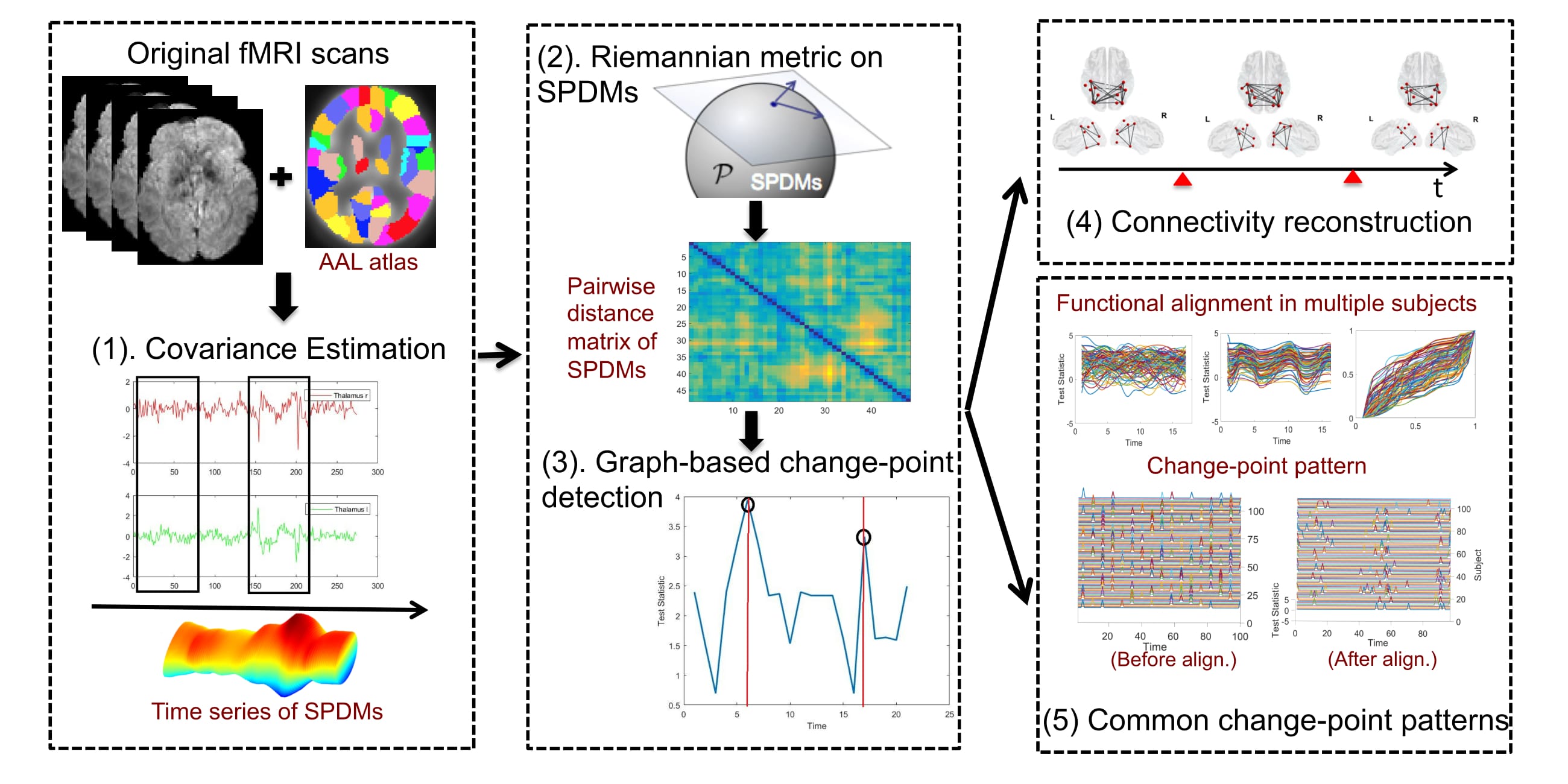
Figure 1: A systematic overview of our proposed framework for FC change-point study.

2.1 FC Estimation Using Covariance Matrices

The first problem is to estimate a correlation or a covariance matrix that represents short-term FC between anatomical regions of interest. To specify this matrix, we pick $n$ ROIs and then represent the FC over a short period using a $n\times n$ covariance matrix of corresponding BOLD signals. In this paper we use the approach from Ledoit and Wolf (2004) to estimate the covariance matrix. Here the estimator $\Sigma_{*}$ is an asymptotically optimal convex linear combination of the sample covariance matrix $S_{*}$ and the identity matrix $I$, i.e. $\Sigma_{*}=\rho_{1}I+\rho_{2}S_{*}$, and the optimal weights $\rho_{1}$ and $\rho_{2}$ are estimated from the data. This estimator is distribution-free and has a simple explicit formula that is easy to compute and interpret. The optimality is defined with respect to a quadratic loss function, valid when the number of observations and the number of variables go to infinity together. Extensive Monte Carlo studies confirms that the asymptotic results tend to hold well even for a reasonable finite sample. Brier et al. (2015) have applied this technique in an analysis of dynamic FC. There are other ways of estimating covariance matrix, see for example Hinne et al. (2015), and we can easily substitute them here as needed.

We segment the original multivariate time series into overlapping blocks of equal size. We will use $W$ as the window size for estimating covariance matrices and $S$ as the step size for sliding windows: $W$ should be large enough to result in a positive definite covariance, but not too large to smooth over subtle changes that are critical to assessments of temporal evolution of FC. Additionally, $S$ should be large enough to reduce dependency in successive covariance matrices for a better change-point detection. These quantities are determined in practice using trial and error, especially with the help of simulated data since the ground truth is available in that situation. This issue is discussed in more detail later in the paper.

2.2 Riemannian Structure on Symmetric Positive-Definite Matrices (SPDMs)

In order to quantify differences in FC, represented by the corresponding covariance matrices, we need a metric structure on the manifold of covariance matrices or SPDMs. While there are several Riemannian structures used in the literature (including one in Pennec et al. (2006)), we briefly summarize the idea used in this paper. More details can be found in Su et al. (2012) and Zhang et al. (2015).

Let ${\mathcal{P}}$ be the space of $n\times n$ SPDMs, and let $\tilde{\cal P}$ be its subset of matrices with determinant one. In this approach one imposes separate distances on the determinant one matrices and the determinants themselves. Recall that for any square matrix $G$ with unit determinant, we can write it as a product of two square matrices $G=PS$, where $P\in\tilde{\cal P}$ and $S\in SO(n)$ ($SO(n)$ is the set of all rotation matrices). This is called the polar decomposition and motivates the analysis of $P$ by representing it as a $G$ after removing $S$. More formally, one obtains a distance on $\tilde{\cal P}$ by identifying it with the quotient space $SL(n)/SO(n)$. This identification is based on the map $\pi:SL(n)/SO(n)\to\tilde{\mathcal{P}}$, given by $\pi([G])=\sqrt{\tilde{G}\tilde{G}^{t}}$, for any $\tilde{G}\in[G]$. The notation $[G]$ stands for all possible rotations of the matrix $G$, given by $[G]=\{GS|S\in SO(n)\}$. The inverse map of $\pi$ is given by: $\pi^{-1}(\tilde{P})=[\tilde{P}]\equiv\{\tilde{P}S|S\in SO(n)\}\in SL(n)/SO(n)$. Skipping further details, this process leads to the following geodesic distance between points in $\tilde{\mathcal{P}}$. For any $\tilde{P}_{1},\tilde{P}_{2}\in\tilde{\mathcal{P}}$:

$$d_{\tilde{\cal P}}(\tilde{P}_{1},\tilde{P}_{2})=\|A_{12}\|,\ \ \mbox{where}\ \ A_{12}=\log(P_{12}),\ \ \ P_{12}=\sqrt{\tilde{P}_{1}^{-1}\tilde{P}_{2}^{2}\tilde{P}_{1}^{-1}}\ .$$ (1)

Since for any ${P}\in{\mathcal{P}}$ we have $\det({P})>0$, we can express ${P}$ as the pair $(\tilde{P},\frac{1}{n}\log(\det({P})))$ with $\tilde{P}=\frac{{P}}{\det({P})^{1/n}}\ \in\tilde{\cal P}$. Thus, ${\mathcal{P}}$ is identified with the product space of $\tilde{\cal P}\times\mathbb{R}$ and we take a weighted combinations of distances on these two components to reach a metric on $\mathcal{P}$:

$$d_{{\mathcal{P}}}(I,{P})^{2}=d_{\tilde{\mathcal{P}}}(I,\tilde{P})^{2}+\frac{1}{n}\ (\log(\det({P})))^{2}.$$ (2)

For any two arbitrary covariances ${P_{1}}$ and ${P_{2}}$, let ${P_{12}}={P_{1}^{-1}}{P_{2}}S_{12}$ for the optimal $S_{12}\in SO(n)$ (using Procrustes alignment). For this ${P_{12}}\in{\mathcal{P}}$, we have $\det({P_{12}})=\det({P_{2}})/\det({P_{1}})$ and define $\tilde{P}_{12}=P_{12}/\det(P_{12})$. Therefore, the resulting squared geodesic distance between ${P_{1}}$ and ${P_{2}}$ is:

$$d_{{\mathcal{P}}}({P_{1}},{P_{2}})^{2}=d_{\tilde{\mathcal{P}}}(I,\tilde{P}_{12})^{2}+\frac{1}{n}\ (\log(\det({P_{2}}))-\log(\det({P_{1}})))^{2}.$$ (3)

Once we have a distance between covariances, we can use that to define and compute sample means on ${\cal P}$ as follows. The sample Karcher or Fréchet mean of a given set of covariances is defined to be:

$$\bar{P}=\arg\min_{{P}\in{\cal P}}\left(\sum_{i=1}^{n}d_{{\mathcal{P}}}({P},P_{i})^{2}\right),$$ (4)

where $\{P_{i}\in{\cal P}\}$ is set of given covariances. The algorithm for computing this mean is a standard one and is not repeated here. We refer the reader to Su et al. (2012) for more details.

2.3 Change-Point Detection Using MST

The next issue is to detect change-points in a SPDM time series using a metric-based approach. We adapt a nonparametric graph-theoretical method introduced by Chen and Zhang (2015) for solving this problem. There have been earlier works on graph-based methods for a two-sample test, but these authors extend the framework to arbitrary metric spaces. Even though this method is theoretically designed for $i.i.d.$ samples from their respective distributions, extensive experiments establish its usefulness even for dependent time series.

Let $X_{1},X_{2},$ $\dots,X_{L}$ be a random, time-ordered sequence taking values on a Riemannian manifold $M$, and let $F_{0}$ and $F_{1}$ denote two probability distribution functions on $M$. We are interested in testing the null hypothesis that all $X_{t}$s are samples from the same distribution, against an alternative that all points before and after a certain time $\tau$ follow different distributions, respectively. That is,

$$H_{0}:X_{t}\sim F_{0},\ t=1,2,\dots,L,\ \ \ \ \ \ \ \ \ \ H_{1}:\exists\ 1\leq\tau<L,\ \ X_{t}\sim\left\{\begin{array}[]{cc}F_{1},&t>\tau\\ F_{0},&\ \ \mbox{otherwise}\ ,\end{array}\right.$$

This test is phrased for a single change-point at time $\tau$, but we will repeat it for different $\tau$s separated by a certain minimum spacing to detect multiple change-points.

The test statistic $Z(\tau)$ for this test is computed as follows. First compute all the pairwise distances between all $\{X_{t}\}$ under the chosen metric on $M$. Then, use these distances to form a minimal spanning tree (MST) connecting the set $\{X_{t}\}$ in $M$. An MST is a connected graph such that: (1) each $X_{t}$ is a node in the graph (i.e., connected to at least one other point in the set, (2) if any two points are connected by an edge then the weight of that edge is given by the pairwise distance between those points, and (3) the sum of weights of all connected edges is the smallest amongst all such graphs. Note that the MST is independent of the ordering of the given points, and can be computed/stored for the whole sequence in one shot. To test whether there is a change-point at $\tau\in\{1,2,\dots,L-1\}$, we divide $X_{t}$s into two groups: $\{X_{1},\dots,X_{\tau}\}$, and $\{X_{\tau+1},\dots,X_{L}\}$. Let $R(\tau)$ represent the number of edges that connect points across these two groups in MST. Intuitively, if $\tau$ is a change-point, with before and after samples being homogeneous in their respective sets, then the two groups represent relatively disjoint clusters of points and only a small number of edges connect across those clusters. In contrast, if the two groups are from the same distribution, then we expect a large number of edges in MST going across the two groups. Chen and Zhang (2015) show that under $H_{0}$, i.e. there is no change-point at $\tau$, the quantity $R(\tau)$ has a distribution with mean and variance given by:

$$E(R(\tau))=p_{1}(\tau)|G|,$$

$$Var(R(\tau))=p_{2}(\tau)|G|+(\frac{1}{2}p_{1}(\tau)-p_{2}(\tau))\sum_{t}|G_{t}|^{2}+(p_{2}(\tau)-{p_{1}}^{2}(\tau))|G|^{2},$$

where $p_{1}(\tau)=\frac{2\tau(L-\tau)}{L(L-1)}$ and $p_{2}(\tau)=\frac{4\tau(\tau-1)(L-\tau)(L-\tau-1)}{L(L-1)(L-2)(L-3)}$. Here, $|G|$ is the total number of edges in $G$ and $|G_{t}|$ is defined as the number of edges in subgraph of $G$ containing all edges that connect to node $X_{t}$. Now, we can standardize $R(\tau)$ using $Z(\tau)=-{(R(\tau)-E(R(\tau))\over\sqrt{Var(R(\tau))}}$ to reach the test statistic. This test statistic is then tested for significance at a given confidence level, for accepting or rejecting the null hypothesis. According to Chen and Zhang (2015), a value of $Z(\tau)\geq 3$ implies a change-point detection at $0.95$ confidence level, and $Z(\tau)\geq 4$ implies a change-point detection at $0.99$ confidence level. One can also use a permutation test to set a threshold for change-points at a certain significant level. However, when using permutation tests on simulated data, we found that the resulting thresholds are actually quite similar to the values stated above. Therefore, we simply use the value of 3 for all experiments in order to save computational cost. The change-point detection process is summarized in Algorithm 1.

Remark 1.

In this setup, the choice of parameters such as $W$, $S$, and $L$ plays an important role. As mentioned previously, $W$ should be large enough to obtain a positive-definite matrix centered at each time, and $S$ should be large enough to avoid the smoothing over of covariance variability. Similarly, $L$ should be large so we have sufficient sample size for change-point detection. On the other hand, it should not to be too large to contain multiple change points in each estimation. In our implementations, we choose these parameters on the basis of overall time length of the fMRI signal $(L_{total}$), number of ROIs ($n$), and these above considerations. Furthermore, we study the effect of changes in $W$ on the detection results and demonstrate that the results are quite stable with respect to this parameter. (One can do the same for $S$ also if the data is rich enough to allow that study, but we expect a similar stability within reasonable limits). So, we have generally used parameter values $W=16$ and $S=6$ in our experiments in which $L_{total}\approx 250$ and $n=4$ to $15$.

Algorithm 1.

Change-Point Detection for SPDM Time Series

1. For a given time ordered set of points $\{X_{t}\in M,t=\tau-0.5L,\tau-0.5L+1,\dots,\tau+0.5L-1\}$, compute $D$, the $L\times L$ pairwise geodesic distance matrix. Here $\tau$ takes value on the set $\{0.5L+1,0.5L+2,\dots,L_{total}-0.5L+1\}$ and $L_{total}$ is the length of the full covariance sequence.

2. Use $D$ to form a minimal spanning tree (MST) connecting all the points.

3. Count $R(\tau)$, the number of edges in this MST between first group: $\{X_{\tau-0.5L},\dots,X_{{\tau}}\}$, and the second group $\{X_{\tau+1},\dots,X_{\tau+0.5L-1}\}$.

4. Calculate $E(R(\tau))$ and $Var(R(\tau))$, and use them to standardize $R(\tau)$, resulting in $Z(\tau)$. At $0.95$ confidence level, use $Z(\tau)\geq 3$ for detecting a change point. By construction, the separation between any two change-points will be at least $W$ in this framework.

5. Set $\tau=\tau+1$ and repeat Step $1$ - Step $4$ until $\tau=L_{total}-0.5L+1$.

   Remark 2.

   Since $Z(\tau)$ can be potentially high for a number of neighboring $\tau$s, we select the local maximizer of $Z(\tau)$ as the detected change-point. That is, we find time points where – function $Z(\tau)$ is increasing before it and decreasing after it.

Before we proceed further, we make the following observations about this MST-based change-point detection:

• This method is theoretically derived for data points that are sampled independently from their respective distributions. However, elements of the SPDM time series under study are seldom independent. Later in the paper we present empirical studies that show that this method also works well for data with dependent structures.

• When we are testing for change-point at a time $\tau$, we assume that the samples before and after $\tau$ are from the same distribution, respectively. In other words, there are no other change-points other than $\tau$. However, as we know, FC over large time intervals can potentially have multiple change-points. We mitigate this issue by using a window-based approach: we choose a large window of a fixed length, say $L$, and test whether the midpoint of that window is a change-point or not. In this way, we do not use the full time-series data for change-point detection at a time $\tau$, we only use data in the vicinity of $\tau$. We repeat the process after moving the large window forward, as shown in Figure 2.

• This graph-based approach is not suitable for detecting change-points at the beginning and at the end of the time series. Therefore, we simply avoid testing these boundary points in our experiments. This is reasonable because the concept of change points is valid only away from the boundaries.

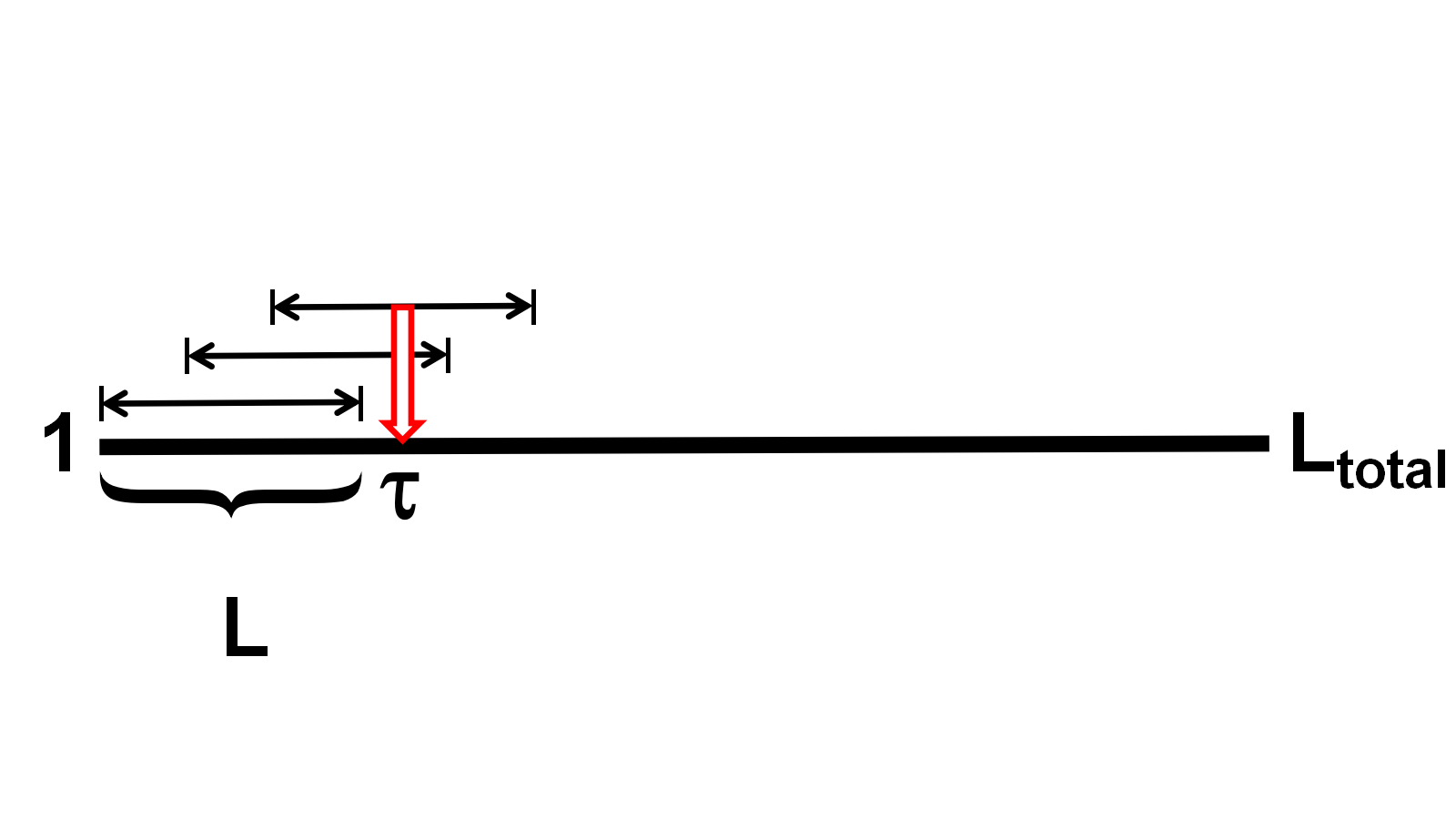
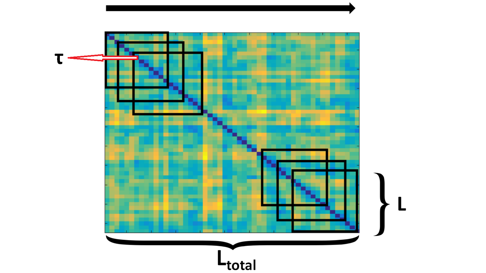
(a)	(b)

Figure 2: (a) An example of a moving window embedded in the sequence of covariance matrices. (b) An example of a moving window embedded in the full distance matrix between all covariance matrices from time $1$ to time $L_{total}$. In each moving window, distance matrix of length $L$ is used to form MST, and change-point test is performed at midpoint $\tau$ in the window.

2.4 Estimation of Connectivity Graphs for Displays

For the purposes of display, one often wants to estimate a graph associated with a FC status. This helps visualize connectivities across regions in a more precise fashion. One needs this, for example, to display brain networks associated with FC over short intervals. Since we are representing FC via a covariance matrix, we face the problem of estimating a network or graph from a covariance matrix. We accomplish this using graphical Lasso (Friedman et al. (2008)), as follows. Let the full observation period be divided into sub-intervals separated by the detected change-points $\tau_{1}$, $\tau_{2}$, etc. For each sub-interval $[\tau_{j},\tau_{j+1})$ we compute the Karcher mean of all SPDMs over this sub-interval, under the Riemannian structure described earlier; call this mean $\bar{P}_{j}\in{\cal P}$. Then, we use this mean SPDM as a representative FC of that subinterval and estimate the associated precision matrix using:

$$\hat{\Theta}_{j}=\underset{\Theta\geq 0}{\operatorname{argmin}}\left(\mbox{tr}(\bar{P}_{j}\Theta)-\log(det(\Theta))+\rho\sum_{i\neq k}{|\Theta_{ik}|}\right),\$$

where $\rho>0$ is a parameter controls density of the generated graph (Figure 3 illustrates the effect of $\rho$ on the resulting graph). Given the estimated precision matrix $\hat{\Theta}_{i}$, the adjacency matrix is obtained by a simple thresholding, i.e. $(A_{j})_{ik}=1_{|\hat{\Theta}_{ik}|>\epsilon=0.001}$. This adjacency matrix is then used to represent the undirected graph formed by the corresponding brain regions. We emphasize that this graph estimation is simply for display purposes and has no bearing on the change-point patterns that we study later.

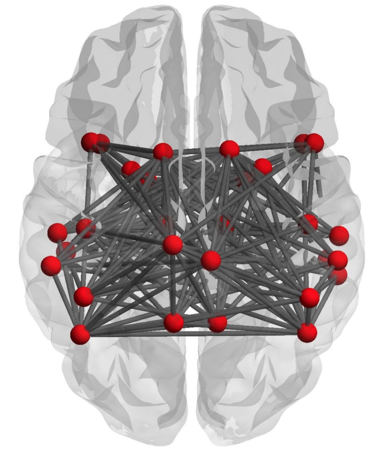
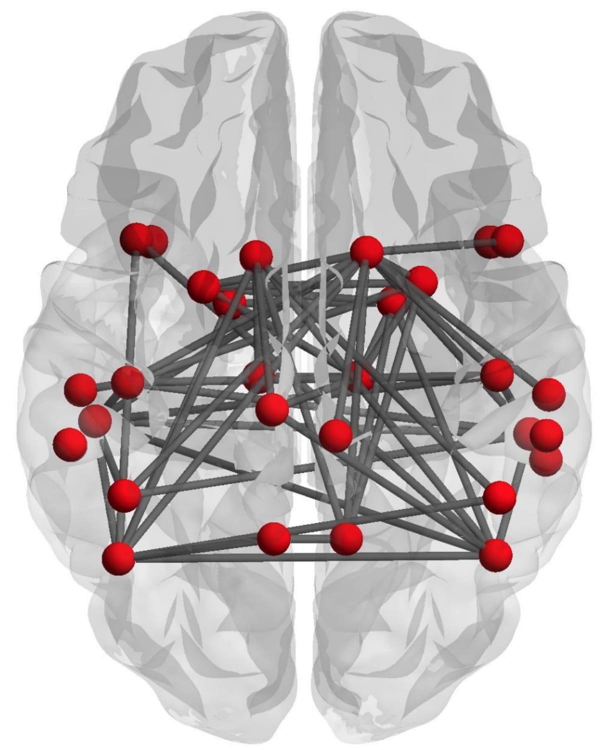
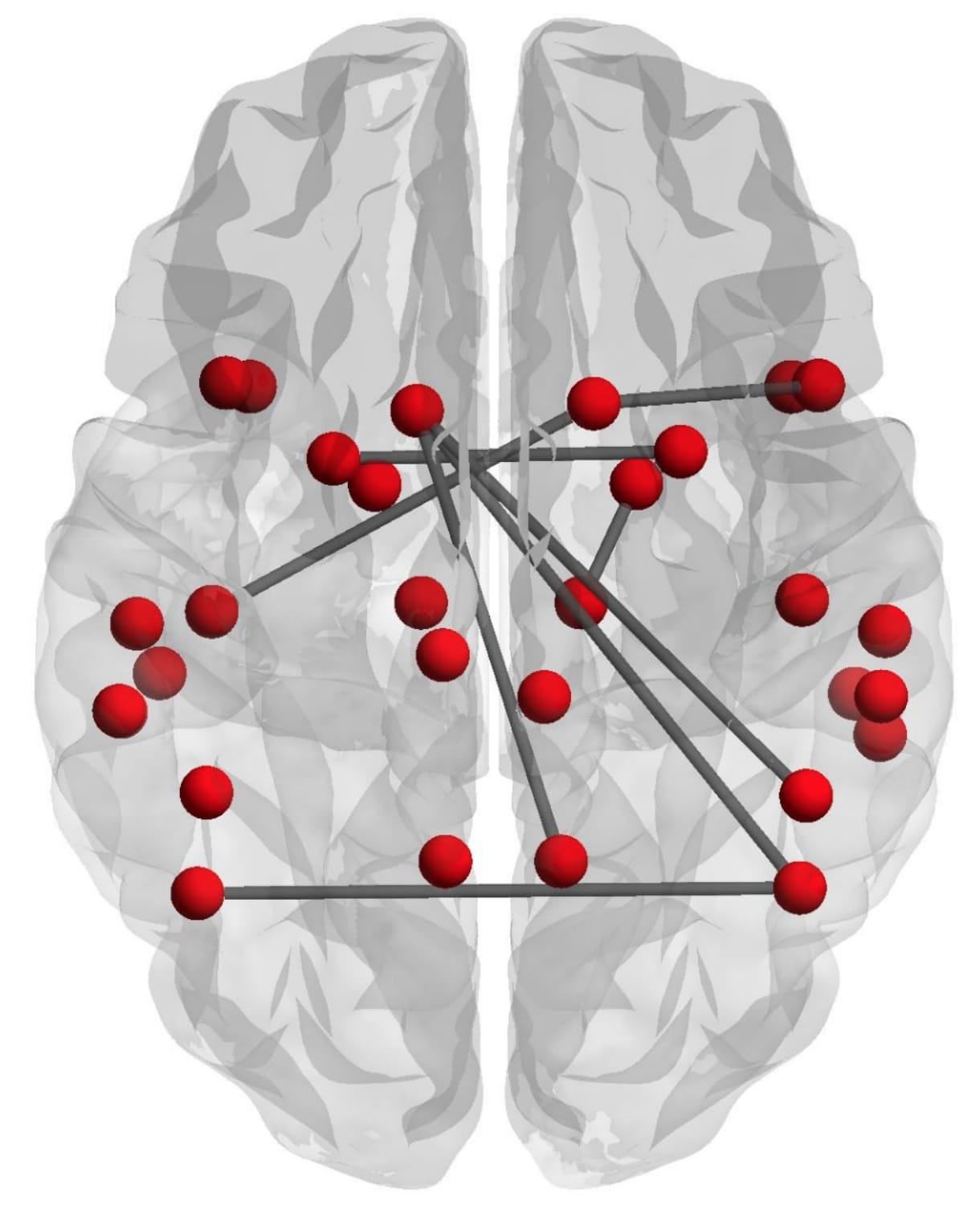
$\rho$=0.01	$\rho$=0.03	$\rho$=0.06

Figure 3: Estimated connectivity of 30 ROIs with different $\rho$s.

We summarize the overall procedure for detecting change-point patterns in FC observations.

Algorithm 2.

Build Stationary Connectivities from fMRI Data

1. Use Algorithm 1, to form a normalized test statistic $Z(\tau)$, for each $\tau\in\{0.5L+1,0.5L+2,\dots,L_{total}-0.5L+1\}$. Make a list of $\tau$s such that $Z(\tau)>3$; call them $\{\tau_{j}\}$. (If several successive $\tau$’s qualify, then we select only the local maximizers of $Z$; see Remark 2.) These selected $\tau$’s denote the change-points of FC over the interval $[0,T]$.

2. For each sub-interval $\{\tau_{j},\tau_{j+1}\}$, find the Karcher mean of covariance matrices $\{P_{\tau_{j}},\dots,P_{\tau_{j+1}}\}$ to form $\bar{P}_{j}$. Use the mean SPDM to estimate the precision matrix and the adjacency matrix, which ultimately forms the brain network for that interval.

3 Temporal Synchronization of Change-Point Statistics

Algorithm 2 enables us to detect change-points and estimate connectivity graphs associated with homogeneous sub-intervals, for each subject individually. Additionally, it provides us with the test statistic $Z(\tau)$ as a probabilistic measure of having a change-point at $\tau$, for each $\tau$ of interest over the interval $[0.5L+1,L_{total}-0.5L]$. Next we are interested in studying patterns of change-points associated with the dynamic FC of a group of individuals when they perform identical or similar tasks. The question is: Are there any change-point patterns that are common across subjects, under such similar experimental conditions? It turns out that simply visualizing $R(\tau)$ for a number of individuals does not lend to any apparent patterns. The reason is that different individuals can have different reaction times for the same external stimulus. Also, in any practical scenario, it is often hard to perfectly align all stimuli. The algorithm used in change-point detection also introduces some variability in detected points. Finally, the randomness of data also leads to variability in strengths and locations of the detected peaks in the test statistic. Together, these factors results in large variability in change point detection results across subjects, reducing the possibility of finding patterns by naked eye. However, if we take into account the temporal variation across individuals, and align these functions to reduce inter-subject variability, a pattern emerges.

To enable temporal registration of test statistics across subjects, we first fit a smooth, densely-sampled function to the discrete $Z(\tau)$ observations of each subject, using cubic splines. Then, we use an elastic method, based on the classical Fisher-Rao metric, to obtain the warping functions that best align these fitted splines across subjects (Srivastava and Klassen (2016)). Let $\{f_{i},i=1,\dots,m\}$, for $m$ subjects, be the set of fitted smooth functions on the observed time interval, e.g. $[0,L_{total}]$. Our goal is to find a set of time warping functions $\{\gamma_{i}\}$, such that $\{f_{i}\circ\gamma_{i}\}$ are temporally aligned as well as possible. Let $\Gamma$ be the set of all positive diffeomorphisms on $[0,L_{total}]$ such that $\gamma(0)=0$ and $\gamma(L_{total})=L_{total}$; its elements play the role of time warping functions. Let $q$ be the square-root slope function (SRSF) of the function $f$, defined as $q(t)=\text{sign}\{\dot{f}(t)\}\sqrt{{|\dot{f}(t)|}}$. (For a detailed description of SRSFs and their use in functional alignment please refer to Chapt 4. of Srivastava and Klassen (2016).) To jointly register functions $\{f_{1},...,f_{m}\}$, the iterative procedure is as follows: initialize a template $\mu_{q}$ and iteratively solve for

$$\gamma_{i}=\arg\inf_{\gamma\in\Gamma}\|\mu_{q}-(q_{i}\circ\gamma)\sqrt{\dot{\gamma}}\|,i=1,2,\cdots,m,\text{and}\ \ \mu_{q}={1\over m}\sum_{i=1}^{m}(q_{i}\circ\gamma_{i})\sqrt{\dot{\gamma}_{i}}\quad.$$ (5)

Each optimization over $\Gamma$ can be solved using the dynamic programming algorithm. We present the alignment algorithm below:

Algorithm 3.

Temporal Alignment of Change-Points

1. Given a set of functions $f_{1},f_{2},...f_{m}$ (smooth functions fitted to the test statistics $Z(\tau)$) on $[0,L_{total}]$, let $q_{1},q_{2},...,q_{m}$ denote their SRSFs, respectively.

2. Initialization step: Select $\mu_{q}=q_{j}$, where $j$ is any index in $\mathop{\rm argmin}_{1\leq i\leq m}\Arrowvert q_{i}-{1\over m}\sum_{k=1}^{m}q_{k}\Arrowvert$ .

3. For each $q_{i}$ find $\gamma_{i}$ by solving: $\gamma_{i}=\mathop{\rm arginf}_{\gamma\in\Gamma}\Arrowvert\mu_{q}-(q_{i}\circ\gamma)\sqrt{\dot{\gamma}})\Arrowvert$. This alignment step is performed using dynamic programming algorithm.

4. Compute the aligned SRSFs $\widetilde{q_{i}}=(q_{i}\circ\gamma_{i})\sqrt{\dot{\gamma}}$.

5. If the increment $\Arrowvert{1\over m}\sum_{i=1}^{m}\widetilde{q_{i}}-\mu_{q}\Arrowvert$ is small, then stop. Else, update the mean using $\mu_{q}={1\over m}\sum_{i=1}^{m}\widetilde{q_{i}}$ and return to step $3$.

6. Compute the mean $\overline{\gamma}={1\over m}\sum_{i=1}^{m}\gamma_{i}$. Center the estimate $\mu_{q}$ with respect to the set $\{q_{i}\}$, according to $\widetilde{\mu_{q}}=(\mu_{q}\circ\overline{\gamma}^{-1})\sqrt{\dot{\overline{\gamma}}^{-1}})$.

7. For i = 1,2,…,m, find $\gamma_{i}$ by solving $\gamma_{i}=\mathop{\rm arginf}_{\gamma\in\Gamma}\Arrowvert\widetilde{\mu_{q}}-(q_{i}\circ\gamma)\sqrt{\dot{\gamma}})\Arrowvert$. Compute the aligned functions as $\widetilde{f_{i}}=(f_{i}\circ\gamma)$.

To demonstrate the effects of alignment, we start with the original test statistic functions $\{Z_{i}\}$ and threshold them to obtain the change-points $\{C_{i}\}$; $\{C_{i}\}$ is a set of binary functions on the interval $[0,L_{total}]$, $1$ at the change-points and $0$ everywhere else. The smooth functions fitted to $\{Z_{i}\}$ are termed $\{f_{i}\}$. From Algorithm 3, we obtain the optimal warping functions $\gamma_{i}^{\prime}s$ to align $f_{i}^{\prime}s$. The aligned functions are denoted by $\{\tilde{f}_{i}=f_{i}\circ\gamma_{i}\}$ and the aligned change-points are given by $\{\widetilde{C}_{i}=C_{i}\circ\gamma_{i}\}$. The $\widetilde{C}_{i}$’s are then used to visualize and discover the change-point patterns across subjects.

4 Experimental Results

In this section we demonstrate our framework using both simulated and real fMRI datasets taken from the Human Connectome Project (HCP) database (Van Essen et al. (2013)).

4.1 Simulation Study

An important use of simulated data analysis is to evaluate methodology in situations where the ground truth is known and can be compared against the quantities estimated from the data. In this section, we simulate data from some simple models that mimic real data settings. We use the popular VAR (Vector Auto Regression) model, in two different state spaces and with a variety of parameter values, in order to study several different scenarios. Since our framework detects change points in covariance trajectories, we can simulate the data either in: (1) the original fMRI signal space and then form covariance trajectories from that simulated data, or (2) the covariance space directly. We will study both the cases in this section. Additionally, we will choose a variety of model parameters in both cases to test the algorithms from different perspectives. Specifically, we will use parameters estimated from the real HCP data and also some randomly selected values to make the evaluation quite comprehensive. With these data settings we demonstrate the success of our method under different parameter choices (window size $W$, step size $S$, larger window $L$, etc) involved in the algorithms.

In terms of the models, we make the following two broad choices:

1. VAR Model in Signal Space: Here we model the data in the original fMRI signal space, generating a time series $\{X_{t}\in\mathbb{R}^{n},t=1,2,\dots,300\}$, where $n$ is the number of ROIs used in the experiment. The VAR(1) model for this case is: $X_{t+1}=A_{t}X_{t}+B_{t}{\cal E}_{t}$, where $A_{t},B_{t}\in\mathbb{R}^{n\times n}$ are time-varying model parameters and ${\cal E}_{t}\in\mathbb{R}^{n}$ is the noise. In all simulation experiments except Experiment 1, we scale the data at each time $t$ by dividing the sum of values in $X_{t}$ at all dimensions, i.e., ${X_{t}}^{(k)}={X_{t}}^{(k)}/(\sum_{j=1}^{n}{X_{t}}^{(j)})$. One can use other methods to normalize such simulated time series data also (Van Poucke et al. (2016)). An example of simulated data in Experiment 1 is shown in Figure 4. One can see that the general scale of values appears similar to the real fMRI data (an example is shown in Figure 1).

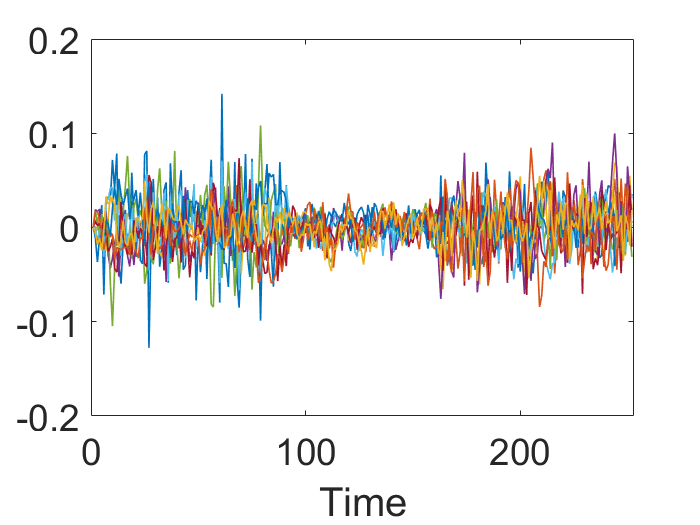
   Figure 4: An example of simulated data from VAR model in signal space when n = 10.

   By choosing different values of $A_{t}$ and $B_{t}$, we explore a variety of scenarios. We deliberately introduce change-points in a time series by dividing the full observation internal into subintervals and by changing model parameters for different intervals. Given a simulated time series under this model, we then compute the corresponding covariance trajectory (using different values of algorithm parameters $W$, $S$, $L$, and $L_{total}$) and study the problem of change-point detection using our approach. In all simulated examples, except when estimating parameters from the real data, we divide the whole time interval $[0,300]$ into three subintervals with change-points located at $100$ and $200$. Also, we use ${\cal E}_{t}\sim{\cal N}(0,0.01*I)$ in the following experiments. Experiments 1-4 are based on data simulated from this data model.

2. VAR Model in Covariance Space: To add variety to the experimental studies, we also model the time series in the covariance space directly, using a model of the type: $P_{t+1}=(A_{t}+B_{t}{\cal E}_{t})P_{t}(A_{t}+B_{t}{\cal E}_{t})^{T}\in\mathcal{P}$. Once again, $A_{t},B_{t}\in\mathbb{R}^{n\times n}$ are model parameters and ${\cal E}_{t}\in\mathbb{R}^{n\times n}$ is a matrix of random observations. Different choices of $A_{t}$ and $B_{t}$ lead to different actual models for the data. We introduce change points in the data by dividing the total time $[0,48]$ into subintervals, with change-points at $17$ and $33$, and use different parameters (but the same model) in different subintervals. Note that one can map this time scale to the time scale of the fMRI signal using $\tau\mapsto(\tau-1)S+W$, where $W=16$ and $S=6$ in most of our experiments. Experiment 5 follows this data model.

In some cases, where we use random SPDMs as parameters in simulation models, first we randomly generate an $n\times n$ square matrix $A_{0}$, then we form an SPDM using $A_{0}{A_{0}}^{T}+nI_{n}$. In both models we make $A_{ij}$s and $B_{ij}s$ unit determinant to prevent time series from going to infinity. Using these two model spaces (and five associated experiments) we perform a number of simulation studies. We simulate the data numerous times, estimate the change-points and collate the results, as described next.

4.1.1 Experiment 1: Simulation using Real Parameters

In this experiment we estimate parameters from real data under the VAR(1) models, and use them to simulate new data. That is, the time series over the $j^{th}$-subinterval, with $j=1,2,3$, is set to be $X_{t+1}=A_{j}X_{t}+\sigma{\cal E}_{t}$, where $A_{j}$s are estimated from HCP data and $\sigma=10$. In practice we tried a number of values of $\sigma$ and found the results to be stable with respect to this choice. The parameters $A_{j}$s are estimated from HCP task data as follows. First we pick $n$ ROIs from single subject gambling task data to form a multivariate time series (in the signal space) and apply Algorithm 1 to detect change-points. We then estimate coefficients $A_{j}$s from a VAR(1) model in each sub-interval, and use these estimated $A_{j}$s to simulate new data $\{X_{t}\}$ using the model mentioned above. Given the simulated data, we implement Algorithm 1 with parameters $W=16$, $S=6$, $L/2=12$, $L_{total}=40$ on this data and the results are noted. We perform this process 1000 times and the estimation summaries (histograms and box plots) of the detected change points are shown in Figure 5. (Note that, for the histograms, we define the change-points to be only the local peaks of the test statistic, as mentioned in Remark 2.) For the box plots, we use the full test statistics (above the chosen threshold of 3), to create a larger data for this summary,

The two rows in Figure 5 correspond to results from two different sets of ROIs (for the same subject and the same task). The top example uses 10 ROIs in CinguloOperc network during the performance of the gambling task. Note that the change-points estimated from the real data, or the ground truth, are located at $t=84,156$. The bottom example comes from 10 ROIs in DorsalAttn network and the ground truth change-points here are located at $t=90,156$. Figure 5(a) shows the evolution of the test statistic $Z(\tau)$ versus $\tau$ on the original real data, while panel (b) shows a histogram of detected test statistic peaks over 1000 simulation runs. The panel (c) shows the corresponding box plot. This last part requires manually separating the two sets of detected points in each run, to designate a change point as either first or second, and we have used $t=130$ for this separation. Together, these two panels show that the estimates are concentrated around true change-point locations. In panel (c) the medians of two change-points are around $t=84$ and $t=156$, coinciding with the true underlying change-points. Similarly, panels (d), (e), and (f) show results associated with the second example. In panel (f) we see the medians of two change-points are located around $t=96,162$, quite close to true change-point locations.

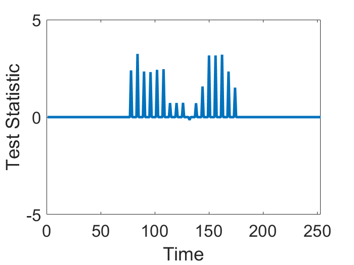
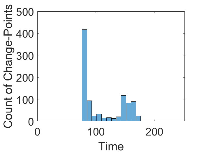
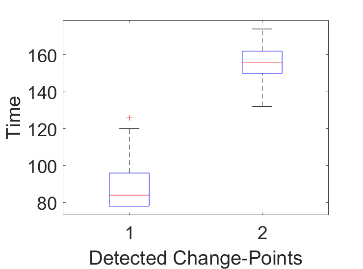
(a)	(b)	(c)
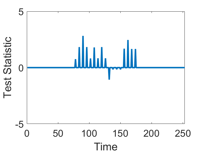
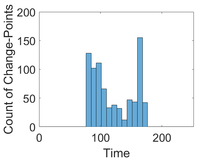
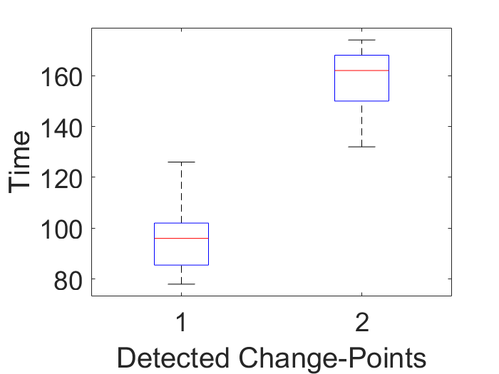
(d)	(e)	(f)

Figure 5: Results of Experiment 1. Top: simulation from 10 ROIs in CinguloOperc network during gambling task. Change-points are located around time $t=84$ and $156$. Bottom: simulation from 10 ROIs in DorsalAttn network during gambling task. Change-points are located around time $t=90$ and $156$. (a), (d) Temporal evolution of the test statistic on real data. (b), (e) Histogram of detected change-points in 1000 simulation runs. (c), (f) Boxplot of these detected change-points.

4.1.2 Experiment 2: Studying Effects of Window Size $W$

In this experiment the goal is to study the effect of the window size $W$ on change-point detection. We simulate the time series over the $j^{th}$-subinterval, with $j=1,2,3$, according to $X_{t+1}=A_{2j}X_{t}+B_{2j}{\cal E}_{t}$, where $A_{21}$ is a randomly-generated, unit-determinant SPDM; $A_{22}=I;A_{23}=2A_{21}-nI;B_{21}=A_{21}+nI;B_{22}=A_{21}+nI;B_{23}=A_{21}+nI$. Once we have the simulated data, we try different values of $W$ (while keeping other algorithmic parameters same) and study the results. In each run, we create a time series with $300$ time points, with $100$ points in each subinterval in a $10$-dimensional space ($n=10$). Here we fix $S=6$, $L/2=12$, and try different values of $W$.

Figure 6 shows a subplots of the test statistics $Z(\tau)$ versus $\tau$ for 12 different values of $W$. Note that due to the correlated nature of the time series data, the high-value of test statistics is not in isolation but is accompanied by a set of high values in its neighborhood. We, thus, find a peak of $Z(\tau)$ value by looking for a local maximum (see Remark 2), i.e. the test statistic is increasing before that value and decreasing after it. The detected change points for these cases are as follows, from top-left to bottom-right: $W=4,t=124;W=8,t=128,206;W=12,t=204;W=16,t=112,208;W=20,t=118,206;W=24,t=120,204;W=28,t=124,208;W=40,t=130;W=44,t=116;W=48,t=126,198.$ The standard deviations of the two detected change-points, across these different $W$s, are found to be $5.92$ and $3.44$, respectively, which highlights the stability of proposed detection method within the chosen range of $W$s. We caution the reader that $W$ should not be too large to smooth over subtle changes that are critical to assessments of temporal evolution of FC (as mentioned in Remark 1).

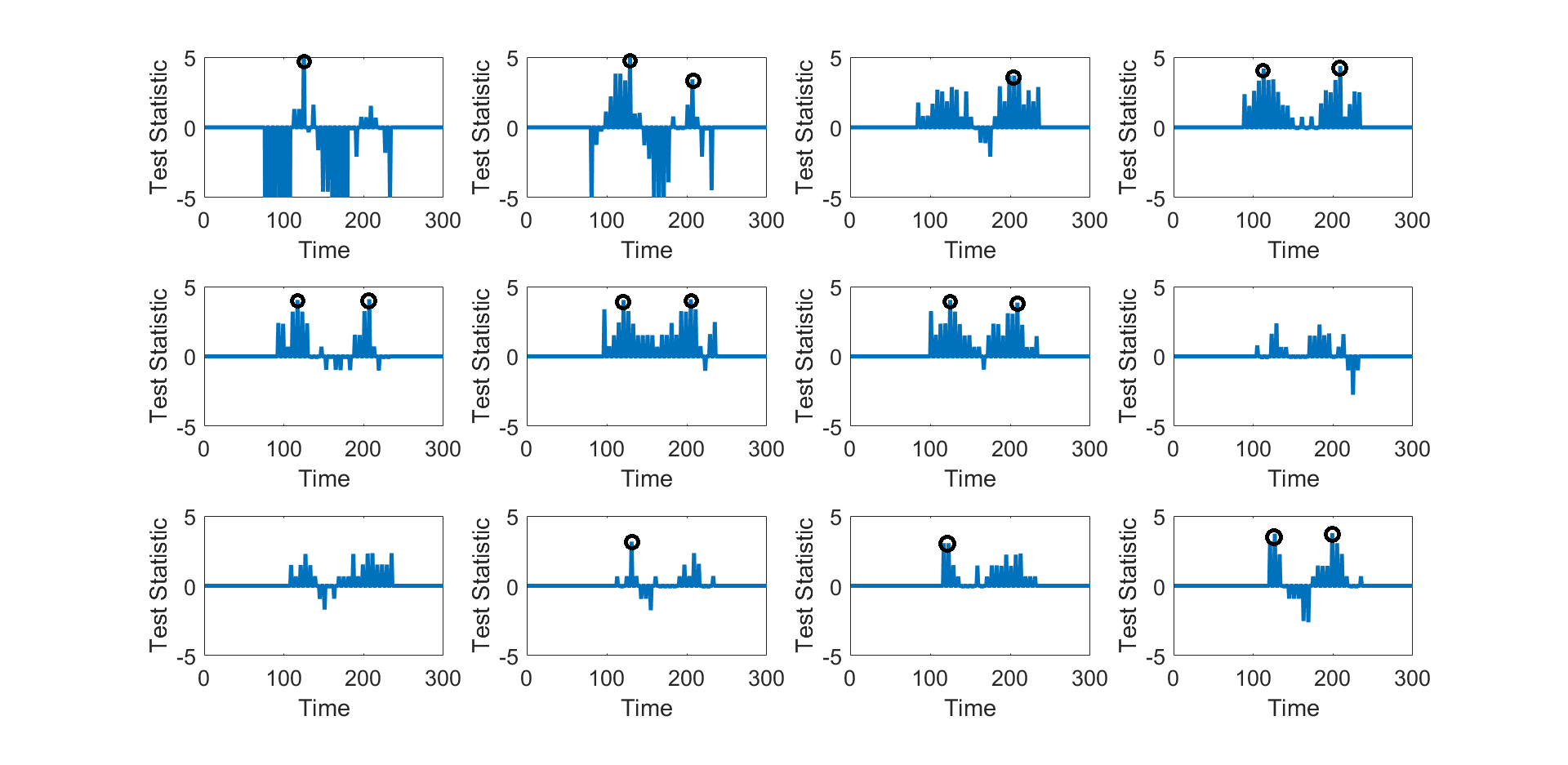
Figure 6: Results of Experiment 2. Change-point detection on simulated data from Model 1.1, with window sizes $W=4,8,12,16,20,24,28,32,36,40,44,48$ from top left to bottom right. The standard deviations of change-point locations for the two change-points are $5.92$ and $3.44$.

4.1.3 Experiment 3: Studying Effects of Increasing $n$

The goal in this experiment is to study the effects of increasing the dimension $n$ on detection results, while keeping the other parameters fixed. To accomplish that, we simulate time series from two sets of model parameters:

• One is the same as in $\bf Experiment$ $\bf 2$, call it Model 1.1.

• The other is $X_{t+1}=A_{3j}X_{t}+B_{3j}{\cal E}_{t}$, call it Model 1.2, where $A_{31}$ is a randomly generated, unit determinant SPDM; $A_{32}=I;A_{33}=2A_{31}+nI;B_{31}=nI;B_{32}=I;B_{33}=J-I$. Here $J$ is an $n\times n$ matrix of all ones.

For each choice of model parameters and $n$, we run the program 100 times and collect the results. Figure 7 shows histograms of detected change-points in each of the settings mentioned in the captions.

We observe that when $n$ is either small or moderate, the algorithm can successfully detect change points with a high degree of accuracy. However, when $n$ gets large, as for example in the case of Model 1.1, $n=50$, the detection algorithm does not perform as well. This is because one needs a larger sample size for estimating larger covariance matrices at the same precision level. This issue can perhaps be mitigated by using different window parameters, or by introducing a dimension reduction technique, but it has not been explored in this paper.

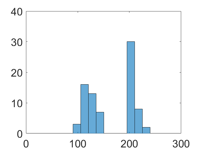
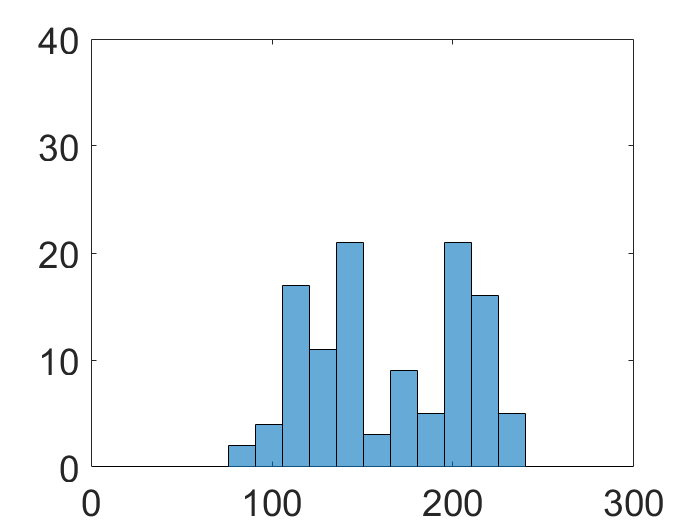
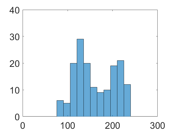
(Model 1.1, $n=4$)	(Model 1.1, $n=15$)	(Model 1.1, $n=50$)
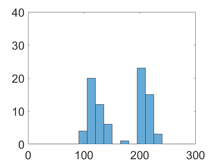
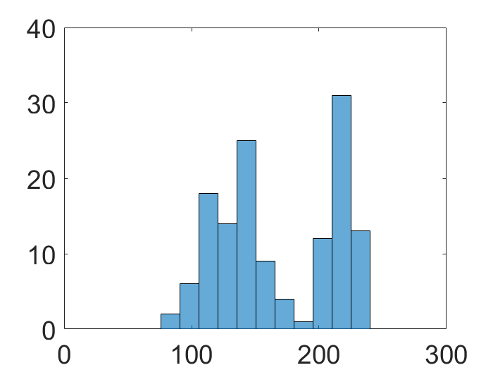
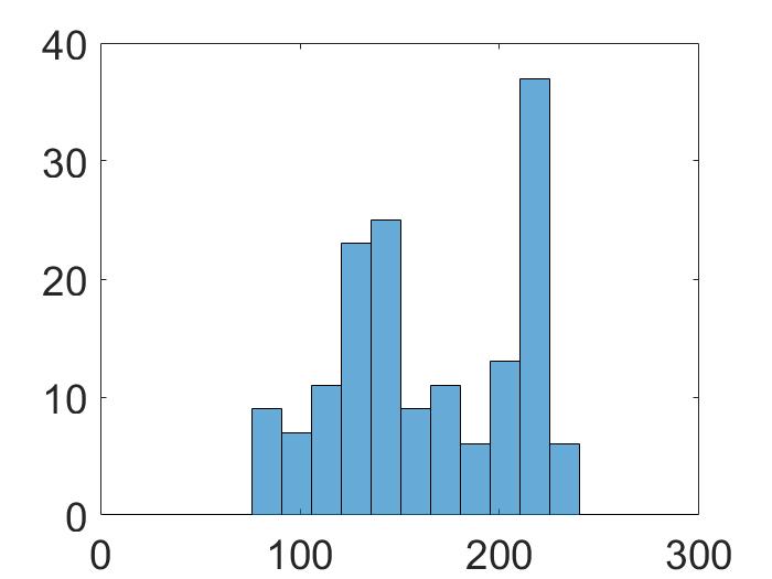
(Model 1.2, $n=4$)	(Model 1.2, $n=15$)	(Model 1.2, $n=50$)

Figure 7: Results of Experiment 3. Histograms of detected change-points given different models and dimensions with 100 runs in each case. Sample means and standard deviations for two change-points in Model 1.1 when n = 4, 15, 50 are (123.15, 11.69; 207.50, 8.88), (125.98, 17.16, 202.08, 20.45), (124.25, 16.35; 200.07, 24.23) respectively; Sample means and standard deviations for two change-points in Model 1.2 when n = 4, 15, 50 are (120.43, 12.70; 210.43.50, 11.61), (126.66, 16.48, 207.54, 24.44), (123.16, 19.40; 202.93, 24.14) respectively.

4.1.4 Experiment 4: Studying Effects of Increasing Temporal Correlations

In this experiment, we study the effects of an increase in temporal correlations of the time series on the detection performance. We use the same model parameters as in ${\bf Experiment\ 2}$, except that we replace $X_{t}$ with $(\sum_{i=1}^{p}X_{t-i+1})/k$, making it a VAR($p$) model. Increasing $k$ increases the correlations in $X_{t}$s across time.

Although the null hypothesis of change-point detection requires independent samples, according to Chen and Zhang (2015), the method still seems quite effective when the data points are weakly dependent. $\bf Experiment$ $\bf 1-3$ use VAR($p$) models with $p=1$, and the state at time $t$ only depends on the state at time $t-1$. Now we increase dependence using VAR(3) and VAR(5) models and study the effects of this dependence on the results. In a VAR(3) model, $X_{t}$ depends on $X_{t-1},X_{t-2},X_{t-3}$, and in a VAR(5) model $X_{t}$ depends on $X_{t-1}$ to $X_{t-5}$. Figure 8 shows histograms of detected change-points in $p=3$ and $p=5$ cases with different values of $n$ and using 100 runs in each setting.

Despite different degrees of dependencies in the data from case to case, our change-point detection algorithm is quite consistent in detecting the original change-points. Even when the dimension gets high, i.e. $n=50$, the process shows a high level of success.

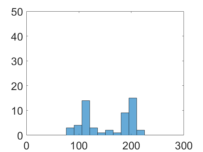
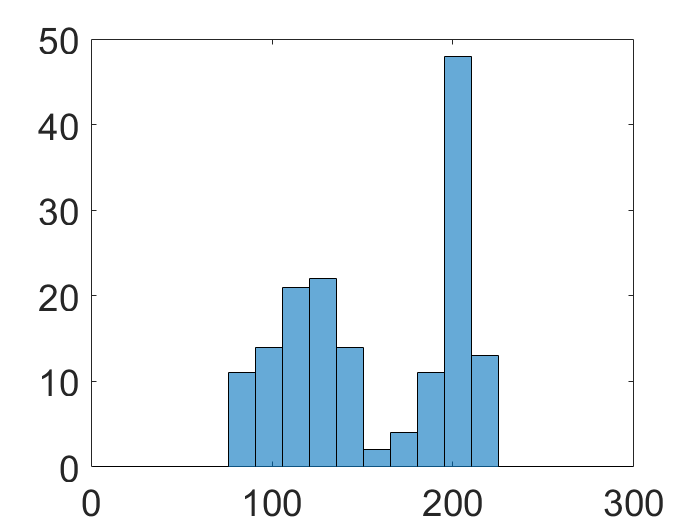
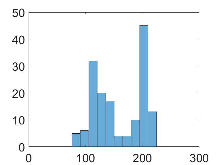
($p=3$, $n=4$)	($p=3$, $n=15$)	($p=3$, $n=50$)
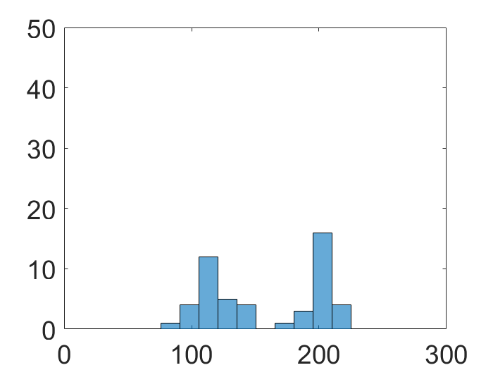
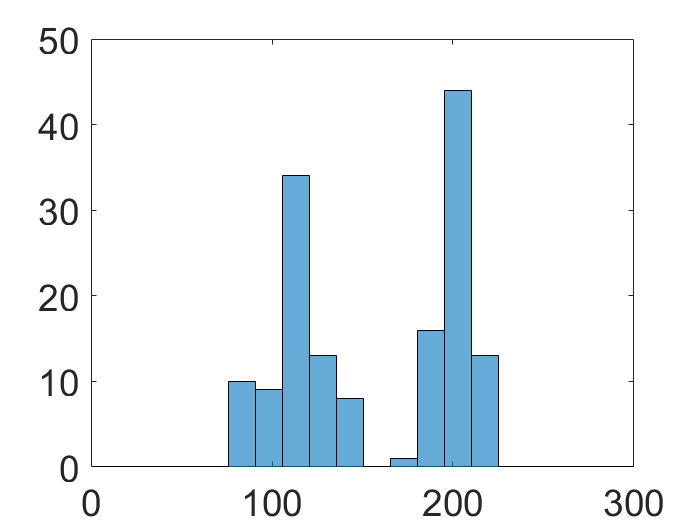
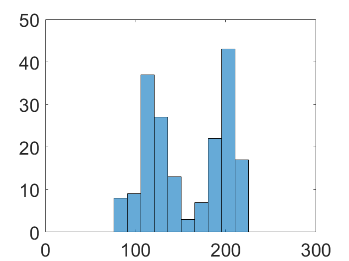
($p=5$, $n=4$)	($p=5$, $n=15$)	($p=5$, $n=50$)

Figure 8: Results of Experiment 4. Histograms of detected change-points given VAR(3) and VAR(5) models with different dimensions with 100 runs in each case. Sample means and standard deviations for two change-points when $p=3,n=4,15,50$ are $(112.56,14.52)$ $(196.14,13.80)$, $(116.05,19.58)$, $(201.85,12.90)$, $(120.23,16.85;200.92,14.88)$ respectively; Sample means and standard deviations for two change-points in Model 1.2 when $p=5,n=4,15,50$ are $(117.23,14.62;203.25.50,9.58)$, $(113.35,17.05,203.51,10.96)$, $(118.60,16.16;199.77,14.22)$ respectively.

4.1.5 Experiment 5: Direct Simulations of Covariance Sequences

In this case, we simulate the time series in ${\cal P}$ directly from two sets of parameters as follows:

• Model 2.1: Using $P_{t}=(A_{4j}+{\cal E}_{t})P_{t-1}({A_{4j}+{\cal E}_{t})}^{T}$, where $A_{41}$ is a randomly generated SPDM; $A_{42}=I;A_{43}=J-I$;

• Model 2.2: Using the same model but different parameters, we have: $P_{t}=(A_{5j}+{\cal E}_{t})P_{t-1}({A_{5j}+{\cal E}_{t})}^{T}$, where $A_{51}=I$, $A_{52}$ is a randomly generated SPDM, and $A_{53}=J-I.$ As earlier, $J$ is an $n\times n$ matrix of ones and ${\cal E}_{t}\sim{\cal N}(0,0.01*I)$.

In Experiments $\bf 2-4$, a signal space series of length $300$ results in a covariance sequence of length $48$ (for $W=16$ and $S=6$). So, for consistency, we simulate covariance sequences of length 48 directly in this case and apply our change-point detection algorithm with $100$ runs in each case. Finally, we map the detected change points back to the signal space time scale (with $300$ points) and display the histograms of detected change-points in Figure 9.

In both the examples, the results show good performance in terms of locations and detection rates when $n$ is low or moderate. When $n$ is high the detection accuracy goes down, highlighting a limitation of the proposed method. As mentioned earlier, we are using a covariance-based representation and one requires more time samples to keep the same level of precision in covariance estimation. Other factors, such as the nature of simulated time series, can also contribute to this lower performance.

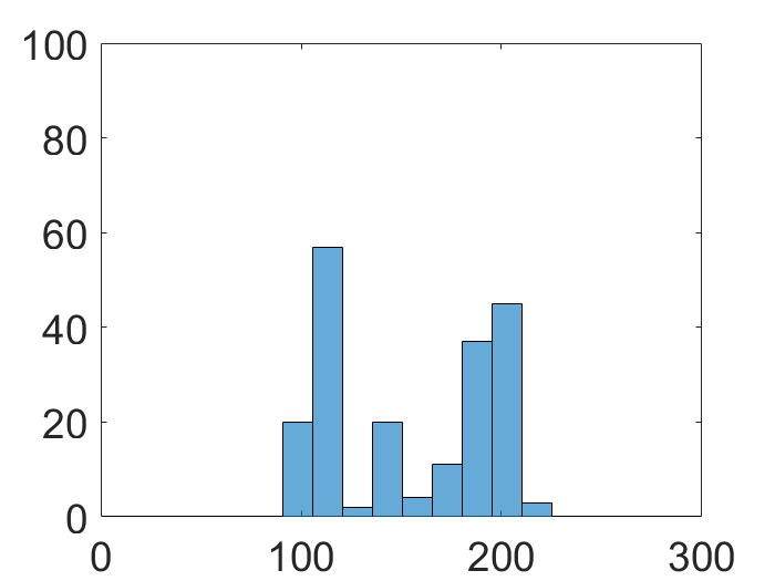
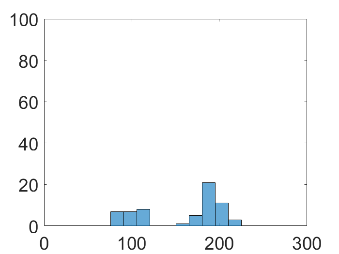
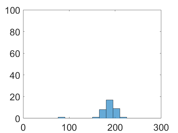
(Model 2.1, $n=4$)	(Model 2.1, $n=15$)	(Model 2.1, $n=50$)
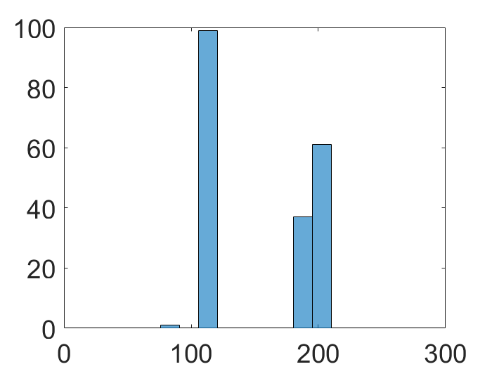
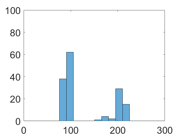
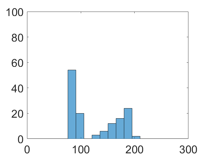
(Model 2.2, $n=4$)	(Model 2.2, $n=15$)	(Model 2.2, $n=50$)

Figure 9: Results of Experiment 5. Histograms of detected change-points given different trajectory models and dimensions with 100 runs in each case. Sample means and standard deviations for two change-points in Model 2.1 when n = 4, 15, 50 are (116.61, 15.57; 193.80, 12.63), (99.27, 12.24, 192.73, 12.31), (78, 0; 189.67, 11.85) respectively; Sample means and standard deviations for two change-points in Model 2.2 when n = 4, 15, 50 are (113.46, 4.19; 196.60, 5.30), (94.44, 7.32, 206.24, 13.14), (94.84, 17.14; 178.11, 12.65) respectively.

4.2 Real Data: Single Subject Dynamic FC

Next we consider task fMRI (tfMRI) data from the HCP database. The majority of the HCP tfMRI data were acquired at 3T, which is considered to be the field strength currently most suitable for acquiring high quality data reliably from a large cohort of subjects. Acquisitions are based on the blood oxygen level dependent (BOLD) contrast. A series of 4D imaging data were acquired for each subject while they were performing tasks involving different neural systems, e.g. visual, motion or cognition systems. The acquired images have an isometric spatial resolution of $2$ mm and temporal resolution of $0.7$s. All fMRI data in HCP are preprocessed by removing spatial distortions, realigning volume to compensate for subject motion, registering the fMRI to the structural MRI, reducing the bias field, normalizing the 4D image to a global mean, masking the data with the final brain mask and aligning the brain to a standard space (Glasser et al. (2013)). This preprocessed tfMRI is now ready for FC analysis.

To map FC, we begin with the segmentation of brain into regions using an existing template, such as the Automated Anatomical Labeling (AAL) atlas (Tzourio-Mazoyer et al. (2002)). Time series for each region in tfMRI are extracted using CONN functional connectivity toolbox (Whitfield-Gabrieli and Nieto-Castanon (2012)) and the default atlas in CONN toolbox. A [0.008, inf] (Hz) high-pass filter is applied to de-noise the time series data. We evaluate dynamic FC using the proposed method for two different tasks: (1) gambling and (2) social cognition. The experimental results are categorized below. We discuss a way of validating these results, later in Section 4.4. Here we present the experimental results as a demonstration of our approach.

1. Gambling Task: The gambling task in HCP was adapted from the one developed in Delgado et al. (2000). Participants play a card guessing game in which they are asked to guess the number on a mystery card in order to win or lose money. Three different type of blocks are presented throughout the task: reward blocks, neutral blocks and loss blocks. Brain regions that naturally relate to this gambling task include basal ganglia, ventral medial prefrontal and orbito-frontal. The basal ganglia contains multiple subcortical nuclei and is the part of brain that influences motivation and action selection. We selected four regions inside the basal ganglia: right Caudate, left Caudate, right Putamen and left Putamen, and studied FC using $4\times 4$ SPDMs representing covariance of fMRI signal in these four regions. Algorithm 2 was applied and the results are shown in Figure 10 (a). It shows the evolution of the test statistic $Z(\tau)$ versus $\tau$ for two different choices of window size $W=16,18$. Despite different window sizes, the algorithm consistently detects the same two change-points, resulting in three subintervals where FC is statistically stationary. For each of these subintervals, we estimated the corresponding connectivity graphs using graphical Lasso and display them in 10(b).

   As another example under the same task – gambling – Figure 11 shows results using 10 ROIs in the Temporal Lobe (including Heschl gyrus, superior temporal gyrus and middle temporal gyrus). This figure shows two detected change-points in (a) and reconstructed graphs for each sub-interval in (b). Compared with the four ROIs case in Figure 10, the change-points detected in Figure 11 are much closer to each other in time. The detection results in these two examples differ because the experiments involve different ROIs and subjects.

   

   Figure 10: Dynamic FC change-point detection for four regions in basal ganglia in gambling task. Peaks in change intervals in (a) are located at $t=90,150$ when $W=16$ and $t=98,176$ when $W=18$.

   (a)	(b)

   Figure 11: FC change-point detection in gambling task for 10 regions in the Temporal Lobe (ROI 78-87). (a) test statistic. Peaks in change intervals are located at $t=126,198$. (b) reconstructed stationary FC networks for the sub-intervals.

2. Social Cognition Task: In this task the participants were presented with short video clips of objects (squares, circles, triangles) that either interact in some way, or moved randomly on the screen (Castelli et al. (2000)). After each video clip, participants judge whether the objects had (i) a mental interaction (an interaction that appears as if the shapes are affecting feelings and thoughts); (ii) not sure or (iii) no interaction. Each run of the task has 5 video blocks (2 Mental and 3 Random in the data used here). Possible brain regions that relate to this task are medial prefrontal cortex, temporal parietal junction, inferior and superior temporal sulcus (Barch et al. (2013)). Since this task has more time blocks (5 blocks) than the gambling data, we expect to detect more change-points. In this example, we used $14$ regions taken from Occipital lobe, Parietal lobe and Temporal lobe, and the algorithm detects several change-points. Figure 12 (a) shows the result using $W=16$. We detected three major change-points and reconstructed the connectivity graphs for these $14$ ROIs within the four sub-intervals of stationary FC. Figure 12 (b) shows the reconstructed networks. We note that the intermediate networks (during intervals 2 and 3) are more complex than the networks at the two ends.

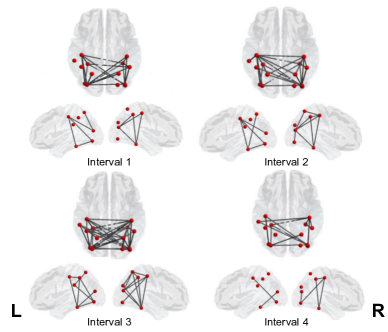
   (a)	(b)

   Figure 12: FC change-point detection in social cognition task for 14 regions (ROI 50-63). (a) change-points with $W=16$. Peaks in change intervals are located at $t=84,138,168$. (b) reconstructed FC networks for the four intervals.

4.3 Real Data: Dynamical FC for Multiple Subjects

Next we use tfMRI data from gambling task and social cognition task to study change patterns across a large set of subjects (197 subjects) from the HCP. As in the earlier experiments, we begin with the segmentation of brain into multiple regions using an existing template as in Gordon et al. (2016). The cortex area is divided into a few networks as visual, auditory, default, frontoparietal, dorsal attention, cingulo-opercular, ventral attention, and salience network. Each network contains several ROIs. One fMRI time series for each selected region is extracted using CONN functional connectivity toolbox (Whitfield-Gabrieli and Nieto-Castanon (2012)). In the following experiments, we used a window size of $W=16$ and a moving step size of $S=6$ (as in previous experiments).

Since it is hard to estimate locations of change-points precisely due to: (1) sliding windows and autocorrelation, and (2) temporal misalignment between subjects, and (3) different response times of individuals to the stimuli in the tasks, we expect that different subjects will have different change-point patterns. The methodology used for change-point detection can also potentially introduce a temporal shift in the detected points. A direct comparison of the raw change-points turns out to be ineffective. After detecting the change-points, we applied Algorithm 3 to reduce the temporal misalignment and to discover the common change-point patterns across subjects. Note that in the following experiments ( labeled as Setup 1-6), we use the same 197 subjects and use the same layout of pictures to present the results (Figure 13-18). Taking Figure 13 as an illustrative example, in panel (a) and (b), we show the raw and aligned detected change-points across 197 subjects. In these panels, each colored line represents the change-point location for an individual subject. Panel (c) shows the smooth functions $\{f_{i}\}$ (fitted to the test statistic curves $\{Z_{i}\}$) before the alignment and panel (d) shows the aligned functions $\{\widetilde{f_{i}}\}$. The corresponding warping functions are displayed in panel (e). The specific ROI names for each figure are given in the supplementary material. We present extensive results using the following experimental setup.

• Setup 1: 12 ROIs are chosen from the CinguloOperc network during the gambling task. The results are shown in Figure 13.

• Setup 2: A different set of 14 ROIs are picked from the DorsalAttn network during gambling task. The results are displayed in Figure 14.

• Setup 3: 12 ROIs (same ROIs as in Setup 1) are used from the CinguloOperc network during the social cognition task. The results are shown in Figure 15.

• Setup 4: 14 ROIs are picked from the DorsalAttn (same ROIs as in Setup 2) network during the social cognition task. Figure 16 shows the results.

• Setup 5: 10 ROIs are picked from the DorsalAttn network during the resting state. The results are shown in Figure 17.

• Setup 6: A different set of 10 ROIs from the VentralAttn network are picked for the resting state data. The results are shown in Figure 18.

  

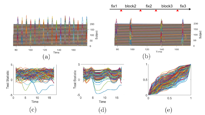
  Figure 13: Change-point patterns of 12 ROIs in the CingulerOperc network during the gambling task for 197 subjects. (a) shows $\{C_{i}\}$ of the detected change-points before alignment, (b) shows $\{\widetilde{C_{i}}\}$ after the alignment, (c) shows the fitted smooth test score functions $\{f_{i}\}$, (d) shows the aligned test score functions $\{\widetilde{f_{i}}\}$ and (e) shows the warping functions for alignment.

  

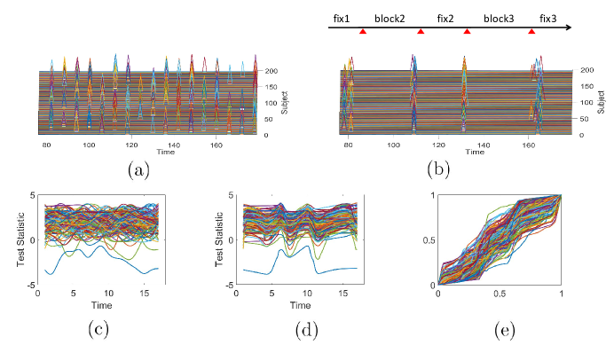
  Figure 14: Change-point patterns of 14 ROIs in the DorsalAttn network during the gambling task for 197 subjects.

  

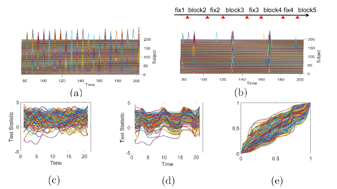
  Figure 15: Change-point patterns of 12 ROIs in the CinguloOperc network during the social task for 197 subjects.

  

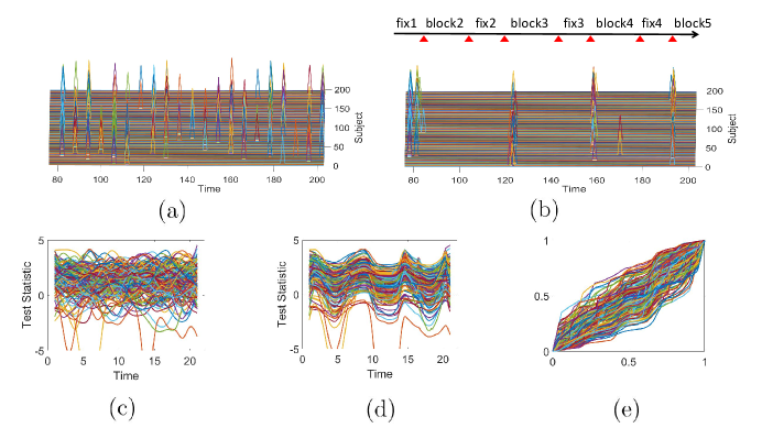
  Figure 16: Change-point patterns of 14 ROIs in the DorsalAttn network during the social task for 197 subjects.

  

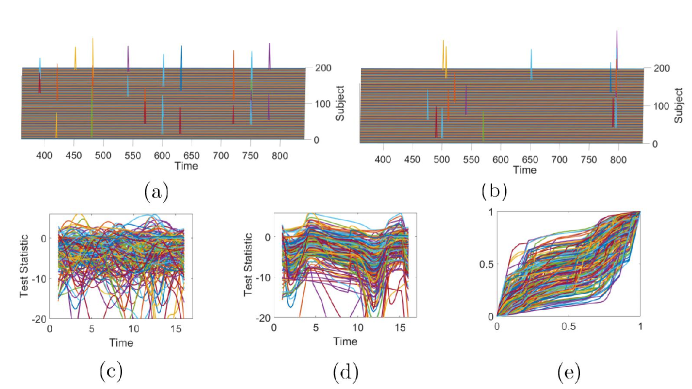
  Figure 17: Change-point patterns of 10 ROIs in the DorsalAttn network during the resting state for 197 subjects.

  

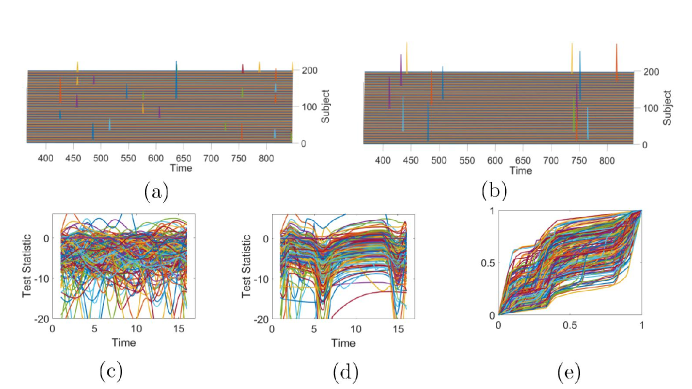
  Figure 18: Change-point patterns of 10 ROIs in the VentralAttn network during the resting state for 197 subjects.

As one can see that the time warping involved in alignment of these datasets is quite significant. While it is difficult to discern any pattern in the original detections, there are certainly common pattens in numbers and locations of change-points across subjects after the alignment in all of these cases.

In order to emphasize the effect of alignment further, we compute and display a matrix of pairwise distances between the test statistic functions of different subjects. In this experiment we take pairwise distances between 394 test statistic functions from both gambling task (first 197 functions) and social task (second 197 functions) for the same 12 ROIs in CinguloOperc network as in Setup 1 and Setup 3. Figure 19 (a) shows the matrix of distances between fitted test statistic functions before alignment ($\{f_{i}\}$), and Figure 19 (b) shows the pairwise distance matrix between fitted test statistic functions after alignment ($\{\widetilde{f_{i}}\}$), using Algorithm 3. In Figure 19 (b) we observe a stronger diagonal block pattern than in Fig. 19 (a), which shows the effect of temporal alignment for task classifications.

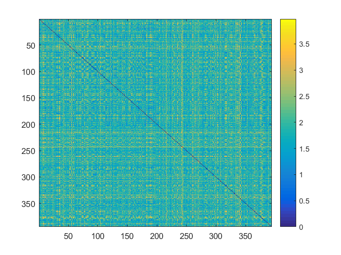
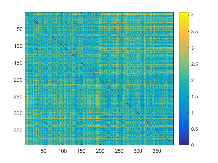
(a)	(b)

Figure 19: Pairwise distances between 394 test statistic functions from both gambling task (first 197 functions) and social task (second 197 functions) given same 12 ROIs in CinguloOperc network. (a) pairwise distances between $f_{i}s$; (b) pairwise distances between $\widetilde{f_{i}}s$.

4.4 Pattern Validation Using Experiment Design Structures

A large number of experiments performed using different tasks and different ROIs combinations reveal common patterns in change-points in FC across subjects. However, an important question is: How can one validate these results in the absence of a ground truth? In this section we take a careful look at the experiment designs and try to compare them with the detected patterns. The overlapping nature of designs blocks and the change-point patterns provide a certain validity to the conclusions.

Let us start with Setup 1 and Setup 2 that are related to the gambling task. The gambling task is presented in blocks of 8 trials that are either mostly reward or mostly loss blocks. In each of the two runs in HCP data acquisition, there are 2 mostly reward and 2 mostly loss blocks, interleaved with 4 fixation blocks (15 seconds each). In Fig. 13 (b), the timeline drawn at the top of the picture gives an example of gambling task blocks taking place, where “fix1” represents the first fixation block, and “block2” represents the second task block (either mostly reward or mostly loss), divided by small red triangles. We can see the aligned change-points mostly take place at intervals between task blocks and fixation blocks. The same holds for the results shown in Fig. 14 (b). In other words, the aligned change-points correspond to the design of the experiment used in collected tfMRI data.

In social task experiments (Setup 3 and Setup 4), our change-point detection model is implemented on the same ROIs as in the gambling task. For this task the participants were presented with short video clips (20 seconds). Each of the two task runs has 5 video blocks and 5 fixation blocks (15 seconds each). In this case we expect to detect more change-points between task or fixation blocks than in gambling task experiments. Comparing Fig. 15 and Fig. 16, we see although the ROIs are the same as in gambling task experiments, the change-point patterns are quite different. Furthermore, the aligned change-points mostly lie in time intervals between task blocks and fixation blocks, given the task timeline at the top of pictures in Fig. 15(b) and Fig. 16(b).

In the remaining two experiments (Setup 5 and Setup 6) we consider the resting state data. These rfMRI data are acquired in four runs of approximately 15 minutes each, two runs in one session and two in another session, with eyes open with relaxed fixation on a projected bright cross-hair on a dark background (and presented in a darkened room). In Fig. 17 and Fig. 18 we observe very few change-points at random time points either before alignment (in (a)) or after alignment (in (b)).

The general correspondence between aligned change-point patterns and experiment block designs, for both gambling and social tasks, can be seen as a validation for our results. The results for resting state experiments where we observe only few change-points also meet our expectation.

5 Conclusion and Discussion

In this paper we have studied patterns of changes in dynamic FC during task-related stimuli across human populations. The methodology consists of a pipeline of techniques used to extract and analyze changes in FC over time for individual subjects. We represent short-term FC as a covariance matrix and model its temporal evolution as a time-series on the manifold of SPDM matrices. Using a Riemannian structure on this manifold, and a graphical approach involving minimal spanning tree, we detect change-points in FC for individual subjects under different tasks and different ROIs. When comparing these detections across subjects, it is difficult to discern common patterns due to the variability introduced by proposed method and misalignment of responses by different people. Using a simple technique for time-warping based alignment of change-point statistics, we are able to visualize similarity of change-point patterns across a large sample of subjects. In order to validate these results, we find general correspondence between these change-point patterns and the block designs of experiments used in the HCP tfMRI data collection.

Our proposed method naturally has some limitations and we list some of them here. One limitation is that the theory in Chen and Zhang (2015) requires i.i.d. samples, while we have applied it to a correlated time series. One should ideally develop a change-point detection approach suited for a time series with dependent samples on a nonlinear manifold. Another limitation is that our method is not suitable for detecting change-points at end points of a time series. This is not a major limitation since the change points are usually meaningful only away from the boundaries. Lastly, since there are several user-specified algorithmic parameters that potentially influence the final result, there may be some variability in the detection results due to these choices. We have used extensive experiments with simulated data and known ground truth to emphasize the success of this approach but we acknowledge this dependence of results on algorithmic choices.

In future, we would like to involve additional datasets in such studies, in order to detect and differentiate patterns from different subpopulations. In order to improve overall performance, we would like to investigate improvements in different pieces of the proposed pipeline. For instance, one can replace the current MST based change-point detection procedure by a method that takes into account the correlated nature of the SPDM time series, as mentioned above.

6 References

References

- Barch et al. (2013) Barch, D., Burgess, G., Harms, M., Petersen, S., Schlaggar, B., Corbetta, M., Glasser, M., Curtiss, S., Dixit, S., Feldt, C., Nolan, D., Bryant, E., Hartley, T., Footer, O., Bjork, J., Poldrack, R., Smith, S., Johansen-Berg, H., Snyder, A., Van Essen, D., 2013. Function in the human connectome: Task-fMRI and individual differences in behavior. NeuroImage 80, 169–189.
- Barnett and Onnela (2016) Barnett, I., Onnela, J.P., 2016. Change point detection in correlation networks. Scientific reports 6, 18893.
- Brier et al. (2015) Brier, M.R., Mitra, A., McCarthy, J.E., Ances, B.M., Snyder, A.Z., 2015. Partial covariance based functional connectivity computation using ledoit-wolf covariance regularization. NeuroImage 121, 29 – 38.
- Castelli et al. (2000) Castelli, F., Happé, F., Frith, U., Frith, C., 2000. Movement and mind: A functional imaging study of perception and interpretation of complex intentional movement patterns. NeuroImage 12, 314 – 325.
- Chen and Zhang (2015) Chen, H., Zhang, N., 2015. Graph-based change-point detection. Ann. Statist. 43, 139–176.
- Cribben et al. (2012) Cribben, I., Haraldsdottir, R., Atlas, L.Y., Wager, T.D., Lindquist, M.A., 2012. Dynamic connectivity regression: Determining state-related changes in brain connectivity. NeuroImage 61, 907 – 920.
- Cribben et al. (2013) Cribben, I., Wager, T., Lindquist, M., 2013. Detecting functional connectivity change points for single-subject fmri data. Frontiers in Computational Neuroscience 7.
- Delgado et al. (2000) Delgado, M., Nystrom, L., Fissell, C., Noll, D., Fiez, J., 2000. Tracking the hemodynamic responses to reward and punishment in the striatum. J. Neurophysiol. 84, 3072–3077.
- Friedman et al. (2008) Friedman, J., Hastie, T., Tibshirani, R., 2008. Sparse inverse covariance estimation with the graphical lasso. Biostatistics 9, 432–441.
- Friston (2011) Friston, K.J., 2011. Functional and effective connectivity: A review. Brain Connectivity 1, 13–36.
- Glasser et al. (2013) Glasser, M., Sotiropoulos, S., Wilson, J., Coalson, T., Fischl, B., Andersson, J., Xu, J., Jbabdi, S., Webster, M., Polimeni, J., Van Essen, D., Jenkinson, M., 2013. The minimal preprocessing pipelines for the Human Connectome Project. NeuroImage 80, 105–124.
- Gordon et al. (2016) Gordon, E.M., Laumann, T.O., Adeyemo, B., Huckins, J.F., Kelley, W.M., Petersen, S.E., 2016. Generation and evaluation of a cortical area parcellation from resting-state correlations. Cerebral Cortex 26, 288–303.
- Hindriks et al. (2016) Hindriks, R., Adhikari, M., Murayama, Y., Ganzetti, M., Mantini, D., Logothetis, N., Deco, G., 2016. Can sliding-window correlations reveal dynamic functional connectivity in resting-state fmri? NeuroImage 127, 242 – 256.
- Hinne et al. (2015) Hinne, M., Janssen, R., Heskes, T., van Gerven, M., 2015. Bayesian estimation of conditional independence graphs improves functional connectivity estimates. PLoS Comput Biol 11, e1004534.
- Hutchison et al. (2013) Hutchison, R., Womelsdorf, T., Allen, E., Bandettini, P., Calhoun, V., Corbett, M., Della Penna, S., Duyn, J., Glover, G., Gonzalez-Castillo, J., Handwerker, D., Keilholz, S., Kiviniemi, V., Leopold, D., de Pasquale, F., Sporns, O., Walter, M., Chang, C., 2013. Dynamic functional connectivity: Promise, issues, and interpretations. NeuroImage 80, 360–378.
- Jeong et al. (2016) Jeong, S.O., Pae, C., Park, H.J., 2016. Connectivity-based change point detection for large-size functional networks. NeuroImage 143, 353 – 363.
- Ledoit and Wolf (2004) Ledoit, O., Wolf, M., 2004. A well-conditioned estimator for large-dimensional covariance matrices. Journal of Multivariate Analysis 88, 365 – 411.
- Lindquist et al. (2014) Lindquist, M., Xu, Y., Nebel, M., Caffo, B., 2014. Evaluating dynamic bivariate correlations in resting-state fmri: A comparison study and a new approach. NeuroImage 101, 531 – 546.
- Monti et al. (2014) Monti, R., Hellyer, P., Sharp, D., Leech, R., Anagnostopoulos, C., Montana, G., 2014. Estimating time-varying brain connectivity networks from functional mri time series. NeuroImage 103, 427 – 443.
- Pennec et al. (2006) Pennec, X., Fillard, P., Ayache, N., 2006. A riemannian framework for tensor computing. Int. J. Comput. Vision 66, 41–66.
- Poldrack (2007) Poldrack, R.A., 2007. Region of interest analysis for fmri. Social Cognitive and Affective Neuroscience 2, 67–70.
- Srivastava and Klassen (2016) Srivastava, A., Klassen, E., 2016. Functional and Shape Data Analysis. Springer.
- Su et al. (2012) Su, J., Dryden, I., Klassen, E., Le, H., Srivastava, A., 2012. Fitting optimal curves to time-indexed, noisy observations on nonlinear manifolds. Journal of Image and Vision Computing 30, 428–442.
- Tzourio-Mazoyer et al. (2002) Tzourio-Mazoyer, N., Landeau, B., Papathanassiou, D., Crivello, F., Etard, O., Delcroix, N., Mazoyer, B., Joliot, M., 2002. Automated anatomical labeling of activations in spm using a macroscopic anatomical parcellation of the mni mri single-subject brain. NeuroImage 15, 273–279.
- Van Essen et al. (2013) Van Essen, D., Smith, S., Barch, D., Behrens, T., Yacoub, E., Ugurbil, K., 2013. The WU-Minn Human Connectome Project: An overview. NeuroImage 80, 62–79.
- Van Poucke et al. (2016) Van Poucke, S., Zhang, Z., Roest, M., Vukicevic, M., Beran, M., Lauwereins, B., Zheng, M.H., Henskens, Y., Lancé, M., Marcus, A., 2016. Normalization methods in time series of platelet function assays: A squire compliant study. Medicine 95, e4188.
- Whitfield-Gabrieli and Nieto-Castanon (2012) Whitfield-Gabrieli, D., Nieto-Castanon, A., 2012. Conn: a functional connectivity toolbox for correlated and anticorrelated brain networks. Brain Connect 2, 125–141.
- Xiao et al. (2017) Xiao, X., Liu, B., Zhang, J., Xiao, X., Pan, Y., 2017. Detecting change points in fmri data via bayesian inference and genetic algorithm model, in: Bioinformatics Research and Applications, Springer International Publishing, Cham. pp. 314–324.
- Xu and Lindquist (2015) Xu, Y., Lindquist, M., 2015. Dynamic connectivity detection: an algorithm for determining functional connectivity change points in fmri data. Frontiers in Neuroscience 9.
- Zhang et al. (2015) Zhang, Z., Su, J., Klassen, E., Le, H., Srivastava, A., 2015. Video-based action recognition using rate-invariant analysis of covariance trajectories. IEEE Transactions on Pattern Analysis and Machine Intelligence in review.