Best Match Graphs and Reconciliation of Gene Trees with Species Trees

Abstract

A wide variety of problems in computational biology, most notably the assessment of orthology, are solved with the help of reciprocal best matches. Using an evolutionary definition of best matches that captures the intuition behind the concept we clarify rigorously the relationships between reciprocal best matches, orthology, and evolutionary events under the assumption of duplication/loss scenarios. We show that the orthology graph is a subgraph of the reciprocal best match graph (RBMG). We furthermore give conditions under which an RBMG that is a cograph identifies the correct orthlogy relation. Using computer simulations we find that most false positive orthology assignments can be identified as so-called good quartets – and thus corrected – in the absence of horizontal transfer. Horizontal transfer, however, may introduce also false-negative orthology assignments.

Keywords: Phylogenetic Combinatorics Colored digraph Orthology Horizontal Gene Transfer

1 Introduction

The distinction between orthologous and paralogous genes has important consequences for gene annotation, comparative genomics, as well as ¡molecular phylogenetics due to their close correlation with gene function (Koonin, 2005). Orthologous genes, which derive from a speciation as their last common ancestor (Fitch, 1970), usually have at least approximately equivalent functions (Gabaldón and Koonin, 2013). Paralogs, in contrast, tend to have related, but clearly distinct functions (Studer and Robinson-Rechavi, 2009; Innan and Kondrashov, 2010; Altenhoff et al., 2012; Zallot et al., 2016). Phylogenetic studies strive to restrict their input data to one-to-one orthologs since these often evolve in an approximately clock-like fashion. In comparative genomics, orthologs serve as anchors for chromosome alignments and thus are an important basis for synteny-based methods (Sonnhammer et al., 2014).

Despite its practical importance, the mathematical interrelationships of empirical “pairwise best hits” on the one hand, and reconciliations of gene and species trees on the other hand have remained largely unexplored. Practical workflows for orthology assignment directly use pairwise best hits as initial estimate of orthologous gene pairs. Many of the commonly used methods for orthology-identification, such as OrthoMCL (Li et al., 2003), ProteinOrtho (Lechner et al., 2014), OMA (Roth et al., 2008), or eggNOG (Jensen et al., 2008), belong to this class. Extensive benchmarking (Altenhoff et al., 2016; Nichio et al., 2017) has shown that these tools perform at least as well as methods such as Orthostrapper (Storm and Sonnhammer, 2002), PHOG (Datta et al., 2009), EnsemblCompara (Vilella et al., 2009), or HOGENOM (Dufayard et al., 2005) that first independently reconstruct a gene tree $T$ and a species tree $S$ and then determine orthologous and paralogous genes.

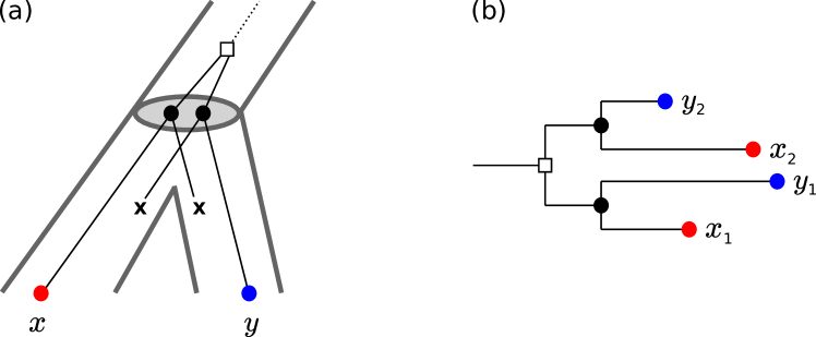
Figure 1: Pairwise best hits are not equivalent to orthology. (a) Complementary losses of ancient paralogs following a later speciation event leaves only a single member of the gene family in each species. Hence, $x$ and $y$ are reciprocal best matches but not orthologs since their last common ancestor by construction is a duplication event. (b) Lineage specific rate differences between paralogs cause discrepancies between best hits and best matches. Here, the branch length in the tree represents sequence dissimilarity. In this example, the species (indicated by the leaf color) retain copies of the two paralogs originating from a duplication event pre-dating the separation of red and blue. While the gene $x_{2}$ evolves faster in the red species, the situation is reversed for $y_{2}$ in the blue species. While $\{x_{1},y_{1}\}$ and $\{x_{2},y_{2}\}$ are orthologs and reciprocal best matches in the evolutionary sense, neither appears as a reciprocal best hit in terms of similarity (i.e., branch length). The only reciprocal best hit is $\{x_{1},y_{2}\}$, which is neither a best match nor a pair of orthologs.

The intuition behind the pairwise best hit approach is that a gene $y$ in species $s$ can only be an ortholog of a gene $x$ in species $r$ if $y$ is the closest relative of $x$ in $s$ and $x$ is at the same time the closest relative of $y$ in $r$. Evolutionary relatedness is defined in terms of an – often unknown – phylogenetic tree $T$. The notion of a best match or closest relative thus is made precise by considering the last common ancestors in $T$: $y$ is a best match for $x$ if the least common ancestor $\operatorname{lca}_{T}(x,y)$ is not further away from $x$ (and thus not closer to the root of the tree) than $\operatorname{lca}_{T}(x,y^{\prime})$ for any other gene $y$ in species $s$. This formally defines the best match relation studied in (Geiß et al., 2019a). The reciprocal best match relation identifies the pairs of genes that are mutually closest relatives between pairs of species, see (Geiß et al., 2019b).

Two approximations are introduced when pairwise best hit approaches are employed for orthology assessment. First, it is well known that two genes can be mutual closest relatives without being orthologs. The usual example is the complementary loss of ancestrally present paralogs following a gene duplication (Fig. 1a). Second, pairwise best hits as determined by sequence (dis)similiarity are not necessarily pairs of most closely related genes and vice versa, evolutionarily most closely related gene pairs do not necessarily appear as pairwise best hits (Fig. 1b).

We argue, therefore, that the relationship of pairwise best hits and orthology has to be understood in (at least) two conceptually and practically separate steps:

1. What is the relationship of pairwise best hits and reciprocal best matches?

2. What is the relation of reciprocal best matches and orthology?

In this contribution we focus on the second question, which is a largely mathematical problem. The first question, which is primarily a question of inference from data, will be investigated in a companion paper that makes use of some of the mathematical results derived here. The main aim of the present contribution is, therefore, to connect formal results on the structure of the orthology relation and the associated reconciliation maps and gene trees with recent results on the mathematical structure of (reciprocal) best match relations.

Symbolic ultrametrics (Böcker and Dress, 1998) and 2-structures (Ehrenfeucht and Rozenberg, 1990a, b) provided a basis to show that orthology relations are essentially equivalent to cographs (Hellmuth et al., 2013, 2017; Hellmuth and Wieseke, 2016). Moreover, in the absence of horizontal gene transfer (HGT), reconciliation maps for an event-labeled gene tree exist if and only if the species tree $S$ displays all triples rooted in a speciation event that have leaves from three distinct species (Hernandez-Rosales et al., 2012; Hellmuth, 2017). This shows that it is possible to infer species phylogenies from empirical estimates of orthology (Hellmuth et al., 2015; Lafond et al., 2016; Lafond and El-Mabrouk, 2014; Dondi et al., 2017). Although it is possible to generalize many of the results, such as the characterization of reconciliation maps for event-labeled gene trees to scenarios with horizontal gene transfer (Nøjgaard et al., 2018; Hellmuth et al., 2019; Hellmuth, 2017) this remains an active area of research.

Best matches as a mathematical structure have been studied only very recently. Geiß et al. (2019a) gave two alternative characterizations of best match digraphs and showed that they can be recognized in polynomial time. In particular, there is a unique least resolved tree for each best match digraph, which is displayed by the gene tree and can also be computed in polynomial time. Reciprocal best matches naturally appear as the symmetric part of these digraphs. Somewhat surprisingly, the undirected reciprocal best match graphs seem to have a much more difficult structure (Geiß et al., 2019b).

Although pairwise best hit methods do not attempt to explicitly construct the gene tree $T$, they still make the assumption that there is some underlying phylogeny for the provided homologous genes. The distinction of orthology and paralogy then amounts to assigning event labels (“speciation”, “duplication”, and possibly “HGT”) to the inner vertices of $T$. While it is true that any gene tree, and thus also any best match graph, can be reconciled with any species tree (Guigó et al., 1996; Page and Charleston, 1997; Górecki and Tiuryn, 2006), such a reconciliation may imply unrealistically many duplication and deletion events. Moreover, the existence of reconciliation maps for $T$ to some species tree cannot generally be ensured, if the event labels are given (Hernandez-Rosales et al., 2012; Hellmuth, 2017). Hence, the best match relation (which constrains the gene tree (Geiß et al., 2019a)), the event labels, the existence of one or a particular reconcilation map, and the species tree depend on each other or at least do constrain each other. In this contribution we explore these dependencies in detail in the absence of horizontal gene transfer.

We show that, in this setting, the true orthology graph (TOG) is a subgraph of the reciprocal best match graph (RBMG). In other words, reciprocal best matches can only produce false positive orthology assignments as long as the evolution of a gene family proceeds via duplications, losses, and speciations. Computer simulations show that in broad parameter range the TOG and RBMG are very similar, proving an a posteriori justification for the use of reciprocal best matches in orthology estimation. In addition, we characterize a subset of the “false positive” edges in the RBMG that cannot be present in the TOG. Experimental results show that – using so-called good quartets – it is possible to remove nearly all false positive orthology assignments. Our aim here is to understand those sources of error and ambiguities in orthology detection that still persist even if reciprocal best matches are inferred with perfect accuracy. Therefore, all computer simulations reported here use perfect data as input. In a companion paper, we address the question how well reciprocal best matches can be inferred from (dis)ssimilarity data, and what can be done to make this inital step more accurate. Finally, we discuss how these results can potentially be generalized to the case that the evolutionary scenarios contain HGT.

2 Preliminaries

A planted (phylogenetic) tree is a rooted tree $T$ with vertex set $V(T)$ and edge set $E(T)$ such that (i) the root $0_{T}$ has degree $1$ and (ii) all inner vertices have degree $\deg_{T}(u)\geq 3$. We write $L(T)$ for the leaves (not including $0_{T}$) and $V^{0}=V(T)\setminus(L(T)\cup\{0_{T}\})$ for the inner vertices (also not including $0_{T}$). To avoid trivial cases, we will always assume that $|L(T)|\geq 2$. The conventional root $\rho_{T}$ of $T$ is the unique neighbor of $0_{T}$. The main reason for using planted phylogenetic trees instead of modeling phylogenetic trees simply as rooted trees, which is the much more common practice in the field, is that we will often need to refer to the time before the first branching event. Conceptually, it corresponds to explicitly representing an outgroup. For some vertex $v\in V(T)$, we denote by $T(v)$ the subtree of $T$ that is rooted in $v$. Its leaf set is $L(T(v))$.

On a rooted tree $T$ we define the ancestor order by setting $x\prec_{T}y$ if $y$ is a vertex of the unique path connecting $x$ with the root $0_{T}$. As usual we write $x\preceq_{T}y$ if $x=y$ or $x\prec_{T}y$. In particular, the leaves are the minimal elements w.r.t. $\prec_{T}$, and we have $x\preceq 0_{T}$ for all $x\in V(T)$. This partial order is conveniently extended to the edge set by defining each edge to be located between its incident vertices, i.e., if $y\prec_{T}x$ and $e=xy$ is an edge, we set $y\prec_{T}e\prec_{T}x$. In this case, we write $e=xy$ to denote that $x$ is closer to the root than $y$. If $e=xy\in E(T)$, we say that $y$ is a child of $x$, in symbols $y\in\mathsf{child}(x)$, and $x$ is the parent of $y$ in $T$. We sometimes also write $y\succeq_{T}x$ instead of $x\preceq_{T}y$. Moreover, if $x\preceq_{T}y$ or $y\preceq_{T}x$ in $T$, then $x$ and $y$ are called comparable, otherwise the two vertices are incomparable.

For a non-empty subset of vertices $A\subseteq V$ of a rooted tree $T=(V,E)$, we define $\operatorname{lca}_{T}(A)$, the last common ancestor of $A$, to be the unique $\preceq_{T}$-minimal vertex of $T$ that is an ancestor of every vertex in $A$. For simplicity we write $\operatorname{lca}_{T}(x_{1},\dots,x_{k})\coloneqq\operatorname{lca}_{T}(\{x_{1},\dots,x_{k}\})$ for a set $A=\{x_{1},\dots,x_{k}\}$ of vertices. The definition of $\operatorname{lca}_{T}(A)$ is conveniently extended to edges by setting $\operatorname{lca}_{T}(x,e)\coloneqq\operatorname{lca}_{T}(\{x\}\cup e)$ and $\operatorname{lca}_{T}(e,f)\coloneqq\operatorname{lca}_{T}(e\cup f)$, where the edges $e,f\in E(T)$ are simply treated as sets of vertices. We note for later reference that $\operatorname{lca}(A\cup B)=\operatorname{lca}(\operatorname{lca}(A),\operatorname{lca}(B))$ holds for non-empty vertex sets $A$, $B$ of a tree.

Binary trees on three leaves are called triples. We say that a triple $xy|z$ is displayed in a rooted tree $T$ if $x,y,$ and $z$ are leaves in $T$ and the path from $x$ to $y$ does not intersect the path from $z$ to the root. The set of all triples that are displayed by the tree $T$, is denoted by $r(T)$ and a triple set $R$ is said to be compatible if there exists a tree $T$ that displays $R$, i.e., $R\subseteq r(T)$.

Denote by $L(S)$ a set of species and denote by $\sigma:L(T)\to L(S)$ the map that assigns to each gene $x\in L(T)$ a species $\sigma(x)\in L(S)$. A tree $T$ together with such a map $\sigma$ is denoted by $(T,\sigma)$ and called leaf-colored tree.

Definition 1.

Let $(T,\sigma)$ be a leaf-colored tree. A leaf $y\in L(T)$ is a best match of the leaf $x\in L(T)$ if $\sigma(x)\neq\sigma(y)$ and $\operatorname{lca}(x,y)\preceq_{T}\operatorname{lca}(x,y^{\prime})$ holds for all leaves $y^{\prime}$ from species $\sigma(y^{\prime})=\sigma(y)$. The leaves $x,y\in L(T)$ are reciprocal best matches if $y$ is a best match for $x$ and $x$ is a best match for $y$.

The directed graph $\mathaccent 382{G}(T,\sigma)$ with vertex set $L(T)$, vertex-coloring $\sigma$, and edges defined by the best matches in $(T,\sigma)$ is known as colored best match graph (BMG) (Geiß et al., 2019a). The undirected graph $G(T,\sigma)$ with vertex set $L(T)$, vertex-coloring $\sigma$, and edges defined by the reciprocal best matches in $(T,\sigma)$ is known as colored reciprocal best match graph (RBMG) (Geiß et al., 2019b). We sometimes write $n$-BMG, resp., $n$-RBMG to specify the number $n$ of colors.

Throughout this contribution, $G=(V,E)$ and $\mathaccent 382{G}=(V,\mathaccent 382{E})$ denote simple undirected and simple directed graphs, respectively. We distinguish directed arcs $(x,y)$ in a digraph $\mathaccent 382{G}$ from edges $xy$ in an undirected graph $G$ or tree $T$. For an undirected graph $G$ we denote by $N(x)=\{y\mid y\in V(G),xy\in E(G)\}$ the neighborhood of some vertex $x$ in $G$. The disjoint union $G\mathbin{\mathchoice{\leavevmode\vtop{\halign{\hfil$\m@th\displaystyle#$\hfil\cr\cup\cr\cdot\crcr}}}{\leavevmode\vtop{\halign{\hfil$\m@th\textstyle#$\hfil\cr\cup\cr\cdot\crcr}}}{\leavevmode\vtop{\halign{\hfil$\m@th\scriptstyle#$\hfil\cr\cup\cr\cdot\crcr}}}{\leavevmode\vtop{\halign{\hfil$\m@th\scriptscriptstyle#$\hfil\cr\cup\cr\cdot\crcr}}}}H$ of two graphs $G=(V,E)$ and $H=(W,F)$ has vertex set $V\mathbin{\mathchoice{\leavevmode\vtop{\halign{\hfil$\m@th\displaystyle#$\hfil\cr\cup\cr\cdot\crcr}}}{\leavevmode\vtop{\halign{\hfil$\m@th\textstyle#$\hfil\cr\cup\cr\cdot\crcr}}}{\leavevmode\vtop{\halign{\hfil$\m@th\scriptstyle#$\hfil\cr\cup\cr\cdot\crcr}}}{\leavevmode\vtop{\halign{\hfil$\m@th\scriptscriptstyle#$\hfil\cr\cup\cr\cdot\crcr}}}}W$ and edge set $E\mathbin{\mathchoice{\leavevmode\vtop{\halign{\hfil$\m@th\displaystyle#$\hfil\cr\cup\cr\cdot\crcr}}}{\leavevmode\vtop{\halign{\hfil$\m@th\textstyle#$\hfil\cr\cup\cr\cdot\crcr}}}{\leavevmode\vtop{\halign{\hfil$\m@th\scriptstyle#$\hfil\cr\cup\cr\cdot\crcr}}}{\leavevmode\vtop{\halign{\hfil$\m@th\scriptscriptstyle#$\hfil\cr\cup\cr\cdot\crcr}}}}F$. Their join has again vertex set $V\mathbin{\mathchoice{\leavevmode\vtop{\halign{\hfil$\m@th\displaystyle#$\hfil\cr\cup\cr\cdot\crcr}}}{\leavevmode\vtop{\halign{\hfil$\m@th\textstyle#$\hfil\cr\cup\cr\cdot\crcr}}}{\leavevmode\vtop{\halign{\hfil$\m@th\scriptstyle#$\hfil\cr\cup\cr\cdot\crcr}}}{\leavevmode\vtop{\halign{\hfil$\m@th\scriptscriptstyle#$\hfil\cr\cup\cr\cdot\crcr}}}}W$ and its edge set is given by $E(G\operatorname{\Join}H)=E\mathbin{\mathchoice{\leavevmode\vtop{\halign{\hfil$\m@th\displaystyle#$\hfil\cr\cup\cr\cdot\crcr}}}{\leavevmode\vtop{\halign{\hfil$\m@th\textstyle#$\hfil\cr\cup\cr\cdot\crcr}}}{\leavevmode\vtop{\halign{\hfil$\m@th\scriptstyle#$\hfil\cr\cup\cr\cdot\crcr}}}{\leavevmode\vtop{\halign{\hfil$\m@th\scriptscriptstyle#$\hfil\cr\cup\cr\cdot\crcr}}}}F\mathbin{\mathchoice{\leavevmode\vtop{\halign{\hfil$\m@th\displaystyle#$\hfil\cr\cup\cr\cdot\crcr}}}{\leavevmode\vtop{\halign{\hfil$\m@th\textstyle#$\hfil\cr\cup\cr\cdot\crcr}}}{\leavevmode\vtop{\halign{\hfil$\m@th\scriptstyle#$\hfil\cr\cup\cr\cdot\crcr}}}{\leavevmode\vtop{\halign{\hfil$\m@th\scriptscriptstyle#$\hfil\cr\cup\cr\cdot\crcr}}}}\{xy\mid x\in V,y\in W\}$. Thus the join of $G$ and $H$ is obtained by connecting every vertex of $G$ to every vertex of $H$.

A class of undirected graphs that plays an important role in this contribution are cographs, which are recursively defined (Corneil et al., 1981):

Definition 2.

An undirected graph $G$ is a cograph if one of the following conditions is satisfied:

• $G=K_{1}$,

• $G=H\operatorname{\Join}H^{\prime}$, where $H$ and $H^{\prime}$ are cographs,

• $G=H\mathbin{\mathchoice{\leavevmode\vtop{\halign{\hfil$\m@th\displaystyle#$\hfil\cr\cup\cr\cdot\crcr}}}{\leavevmode\vtop{\halign{\hfil$\m@th\textstyle#$\hfil\cr\cup\cr\cdot\crcr}}}{\leavevmode\vtop{\halign{\hfil$\m@th\scriptstyle#$\hfil\cr\cup\cr\cdot\crcr}}}{\leavevmode\vtop{\halign{\hfil$\m@th\scriptscriptstyle#$\hfil\cr\cup\cr\cdot\crcr}}}}H^{\prime}$, where $H$ and $H^{\prime}$ are cograph.

An undirected graph is a cograph if and only if it does not contain an induced $P_{4}$ (path on four vertices) (Corneil et al., 1981).

Every cograph $G$ is associated with a set of phylogenetic trees $\mathfrak{T}_{G}$, usually referred to as the cotrees of $G$. Every cotree $T_{G}\in\mathfrak{T}_{G}$ correspond to a possible recursive construction of $G$. Since both the disjoint union and the join operation is associative, it is possible to join or unify two or more component cographs in a single construction step. The leaves of $T_{G}$ correspond to the vertices of $G$. Each interior vertex of $T_{G}$ corresponds to either a join or a disjoint union operation. Its child-subtrees, furthermore, are exactly the cotrees of the component cographs that are joined or disjointly unified, respectively. The event type associated with an inner vertex $u$ will be denoted by $t_{G}(u)$. Each vertex $u$ of $T_{G}$ can be associated with an induced subgraph $G[L(T_{G}(u))]$. A cotree $T_{G}$ is called discriminating if any two adjacent inner nodes represent different types of events. If $T_{G}\in\mathfrak{T}_{G}$ and $T_{G}^{\prime}$ is obtained from $T_{G}$ by contracting a non-discriminating edge, i.e., an edge $uv$ with $t_{G}(u)=t_{G}(v)$, then $T_{G}^{\prime}\in\mathfrak{T}_{G}$. Every cograph has a unique discriminating cotree, which is obtained from any of its cotrees by contracting all non-discriminating edges (Corneil et al., 1981). We note, finally, that the discriminating cotree of $G$ coincides with the modular decomposition tree of $G$.

3 Reconciliation Maps, Event Labelings, and Orthology Relations

A gene tree $T=(V,E)$ and a species tree $S=(W,F)$ are planted phylogenetics trees on a set of (extant) genes $L(T)$ and species $L(S)$, respectively. We assume that we know which gene comes from which species. Mathematically, this knowledge is represented by a map $\sigma\colon L(T)\to L(S)$ that assigns to each gene the species in whose genome it resides. Best match approaches start from a set of genes taken from a set of species. Hence, the “gene-species-association” is known. Moreover, species without sampled genes do not affect the best match graph and we can w.l.o.g. assume that $\sigma$ is a surjective map to avoid trivial cases. Note, however, that the definitions and results presented below naturally extend to general maps $\sigma$. We write $(T,\sigma)$ for a gene tree with given map $\sigma$.

An evolutionary scenario comprises a gene tree and a species tree together with a map $\mu$ from $T$ to $S$ that identifies the locations in the species tree $S$ at which evolutionary events took place that are represented by the vertices of the gene tree $T$. The properties of the map $\mu$ of course depend on which types of evolutionary events are considered. In order to model evolutionary scenarios we assume that evolutionary events of different types do not occur concurrently. In particular, speciation and duplication are always strictly temporally ordered. Gene duplications therefore always occur along the edges of the species tree. Vertices on $T$ that model speciation events, on the other hand, must be mapped to inner vertices of $S$.

From here on we will consider only Duplication/Loss secenarios, that is we explicitly exclude horizontal gene transfer (HGT). We will briefly discuss the effects of HGT in Section 8.

Definition 1 (Reconciliation Map).

Let $S=(W,F)$ and $T=(V,E)$ be two planted phylogenetic trees and let $\sigma\colon L(T)\to L(S)$ be a surjective map. A reconciliation from $(T,\sigma)$ to $S$ is a map $\mu\colon V\to W\cup F$ satisfying

(R0)

Root Constraint. $\mu(x)=0_{S}$ if and only if $x=0_{T}$.

(R1)

Leaf Constraint. If $x\in L(T)$, then $\mu(x)=\sigma(x)$.

(R2)

Ancestor Preservation. $x\prec_{T}y$ implies $\mu(x)\preceq_{S}\mu(y)$.

(R3)

Speciation Constraints. Suppose $\mu(x)\in W^{0}$.

• $\mu(x)=\operatorname{lca}_{S}(\mu(v^{\prime}),\mu(v^{\prime\prime}))$ for at least two distinct children $v^{\prime},v^{\prime\prime}$ of $x$ in $T$.

• $\mu(v^{\prime})$ and $\mu(v^{\prime\prime})$ are incomparable in $S$ for any two distinct children $v^{\prime}$ and $v^{\prime\prime}$ of $x$ in $T$.

Several alternative definitions of reconciliation maps for Duplication/Loss scenarios have been proposed in the literature, many of which have been shown to be equivalent. Nevertheless, we add yet another one because earlier variants do not clearly separate conditions pertaining to the structural congruence of gene tree and species tree (Axioms (R0), (R1), and (R2)) from conditions that (implicitly) distinguish event types, here (R3.i) and (R3.ii). This axiom system also generalizes easily to situations with horizontal transfer as we shall see in Section 8. We proceed by showing that it is equivalent to axioms that are commonly used in the literature, see e.g. Górecki and Tiuryn (2006); Vernot et al. (2008); Doyon et al. (2011); Rusin et al. (2014); Hellmuth (2017); Nøjgaard et al. (2018), and the references therein.

Lemma 1.

Let $\mu$ be a map from $(T=(V,E),\sigma)$ to $S=(W,F)$ that satisfies (R0) and (R1). Then, $\mu$ satisfies Axioms (R2) and (R3) if and only if $\mu$ satisfies

(R2’)

Ancestor Constraint.
Suppose $x,y\in V$ with $x\prec_{T}y$.

• If $\mu(x),\mu(y)\in F$, then $\mu(x)\preceq_{S}\mu(y)$,

• otherwise, i.e., at least one of $\mu(x)$ and $\mu(y)$ is contained in $W$, $\mu(x)\prec_{S}\mu(y)$.

• Inner Vertex Constraint.
  If $\mu(x)\in W^{0}$, then

  • $\mu(x)=\operatorname{lca}_{S}(\sigma(L(T(x))))$ and

  • $\mu(v^{\prime})$ and $\mu(v^{\prime\prime})$ are incomparable in $S$ for any two distinct children $v^{\prime}$ and $v^{\prime\prime}$ of $x$ in $T$.

Proof.

Assume first that (R2) and (R3) are satisfied for $\mu$.
Then property (R2’.i) is satisfied since it is the restriction of (R2) to $\mu(x),\mu(y)\in F$.
To see that (R2’.ii) holds, let $x\prec_{T}y$ and $\mu(x)\in W$ or $\mu(y)\in W$. Assume first that $\mu(y)\in W$. Property (R2) implies $\mu(x)\preceq_{S}\mu(y)$. Let $v$ be the child of $y$ that lies on the path from $y$ to $x$ in $T$, i.e., $x\preceq_{T}v\prec_{T}y$. Assume for contradiction that $\mu(x)=\mu(y)$. By Property (R2) we have $\mu(x)=\mu(v)=\mu(y)$. For every other child $v^{\prime}$ of $y$, Property (R2) implies $\mu(v^{\prime})\preceq_{S}\mu(y)=\mu(v)$. Thus, $\mu(v)$ and $\mu(v^{\prime})$ are comparable; a contradiction to (R3.ii). Hence, $\mu(x)\prec_{S}\mu(y)$ and (R2’.ii) is satisfied. Now suppose $\mu(x)\in W$ and assume for contradiction that $\mu(x)=\mu(y)$. Thus $\mu(y)\in W$ and we can apply the same arguments as above to conclude that (R3.ii) is not satisfied. Hence, $\mu(x)\prec_{S}\mu(y)$ and (R2’.ii) is satisfied.
In order to show that (R3’) is satisfied, let $x\in V$ such that $\mu(x)\in W^{0}$. Properties (R3’.ii) and (R3.ii) are equivalent. It remains to show that (R3’.i) is satisfied. From (R2) we infer $\mu(y)\preceq_{S}\mu(x)$ for all $y\in\bigcup_{v\in\mathsf{child}(x)}L(T(v))=L(T(x))$. Thus,

$$\operatorname{lca}_{S}(\sigma(L(T(x))))\preceq\mu(x).$$ (1)

Property (R3.i) implies that there are two distinct children $v^{\prime},v^{\prime\prime}\in\mathsf{child}(x)$ with $\mu(x)=\operatorname{lca}_{S}(\mu(v^{\prime}),\mu(v^{\prime\prime}))$. Again using (R3.ii), we know that the images $\mu(v^{\prime})$ and $\mu(v^{\prime\prime})$ are incomparable in $S$. The latter together with $\mu(y)\preceq_{S}\mu(v^{\prime})$ for all $y\in L(T(v^{\prime}))$ and $\mu(y^{\prime})\preceq_{S}\mu(v^{\prime\prime})$ for all $y^{\prime}\in L(T(v^{\prime\prime}))$ implies

$$\operatorname{lca}_{S}(\mu(v^{\prime}),\mu(v^{\prime\prime}))=\operatorname{lca}_{S}(\sigma(L(T(v^{\prime})))\cup\sigma(L(T(v^{\prime\prime}))))\preceq_{S}\operatorname{lca}_{S}(\sigma(L(T(x)))).$$

In summary, $\operatorname{lca}_{S}(\sigma(L(T(x))))\preceq_{S}\mu(x)=\operatorname{lca}_{S}(\mu(v^{\prime}),\mu(v^{\prime\prime}))\preceq_{S}\operatorname{lca}_{S}(\sigma(L(T(x))))$ implies that $\mu(x)=\operatorname{lca}_{S}(\sigma(L(T(x))))$ and Property (R3’.i) is satisfied.
Therefore, (R2) and (R3) imply (R2’) and (R3’).

Conversely, assume now that (R2’) and (R3’) are satisfied for $\mu$. Clearly (R2’) implies (R2), and (R3’.ii) implies (R3.ii). It remains to show that (R3.i) is satisfied. Let $\mu(x)\in W^{0}$. By (R2’.ii) we have $\mu(x)\succ_{S}\mu(v_{i})$ for all children $v_{i}\in\mathsf{child}(x)=\{v_{1},\dots,v_{k}\}$, $k\geq 2$. Therefore, $\mu(x)\succeq_{S}\operatorname{lca}_{S}(\mu(v_{1}),\dots,\mu(v_{k}))$. By (R3’.ii), the images $\mu(v_{1}),\dots,\mu(v_{k})$ are pairwise incomparable in $S$. The latter and (R2’.i) imply $\operatorname{lca}_{S}(\mu(v_{1}),\dots,\mu(v_{k}))=\operatorname{lca}_{S}(\bigcup_{i=1}^{k}\sigma(L(T(v_{i}))))=\operatorname{lca}_{S}(\sigma(L(T(x))))=\mu(x)$. It is easy to verify that $\operatorname{lca}_{S}(\mu(v_{1}),\dots,\mu(v_{k}))=\operatorname{lca}_{S}(\mu(v^{\prime}),\mu(v^{\prime\prime}))$ for at least two children $v^{\prime},v^{\prime\prime}\in\mathsf{child}(x)$ is always satisfied. Hence, $\mu(x)=\operatorname{lca}_{S}(\mu(v^{\prime}),\mu(v^{\prime\prime}))$ for some $v^{\prime},v^{\prime\prime}\in\mathsf{child}(x)$ and thus, (R3.i) is satisfied.
Therefore, (R2’) and (R3’) imply (R2) and (R3). ∎∎

A reconciliation map $\mu$ from $(T,\sigma)$ to a species tree $S$ implicitly determines whether an inner node of $T$ corresponds to a speciation or a duplication. Since we assume that distinct events are represented by distinct nodes of the gene tree, all duplication events are mapped to the edges of $S$. Vertices of $T$ mapped to vertices of $S$ thus represent speciations. We formalize this idea as follows:

Definition 2.

Given a reconciliation map $\mu$ from $(T,\sigma)$ to $S$, the event labeling on $T$ (determined by $\mu$) is the map $t_{\mu}:V(T)\to\{\circledcirc,\odot,\newmoon,\square\}$ given by:

$$t_{\mu}(u)=\begin{cases}\circledcirc&\,\text{if }u=0_{T}\text{, i.e., }\mu(u)=0_{S}\text{ (root)}\\ \odot&\,\text{if }u\in L(T)\text{, i.e., }\mu(u)\in L(S)\text{ (leaf)}\\ \newmoon&\,\text{if }\mu(u)\in V^{0}(S)\text{ (speciation)}\\ \square&\,\text{else, i.e., }\mu(u)\in E(S)\text{ (duplication)}\\ \end{cases}$$

The symbols $\circledcirc$ and $\odot$ identify the planted root $0_{T}$ and the leaves of $T$, respectively. Inner vertices are labeled $\square$ for duplication and $\newmoon$ for speciation, respectively.

The event labeling $t_{\mu}$, by definition, is completely determined by a reconciliation map $\mu$. This raises two related questions: (1) which pattern of event labels can arise for reconciliation maps, and (2) what restriction does a given event labeling impose on the reconciliation map? To study these questions, we consider event-labeled trees $(T,t)$ where the event labeling of $T$ is a map $t:V(T)\to\{\circledcirc,\odot,\newmoon,\square\}$ satisfying $t(0_{T})=\circledcirc$, $t(x)=\odot$ for all $x\in L(T)$, and $t(x)\in\{\square,\newmoon\}$ for $x\in V^{0}(T)$. We interpret $\square$ as gene duplication event and $\newmoon$ as speciation event.

A simple consequence of the Axioms (R0)-(R3) is the following result which is stated here for later reference. For the sake of completeness, we also provide a short proof.

Lemma 2.

Let $\mu$ be a reconciliation map from the leaf-colored tree $(T,\sigma)$ to $S=(W,F)$ and $x\in V(T)$ a vertex with $\mu(x)\in W^{0}$. Then, $\sigma(L(T(v^{\prime})))\cap\sigma(L(T(v^{\prime\prime})))=\emptyset$ for any two distinct $v^{\prime},v^{\prime\prime}\in\mathsf{child}(x)$.

Proof.

Assume for contradiction that there is a vertex $z\in\sigma(L(T(v^{\prime})))\cap\sigma(L(T(v^{\prime\prime})))$. By Condition (R2’), we have $\mu(x)\succ_{S}\mu(v^{\prime})\succeq_{S}z$ and $\mu(x)\succ_{S}\mu(v^{\prime\prime})\succeq_{S}z$. Thus, there is a path $P_{1}$ from $\mu(x)$ to $z$ that contains $\mu(v^{\prime})$ and a path $P_{2}$ from $\mu(x)$ to $z$ that contains $\mu(v^{\prime\prime})$. However, Condition (R3.ii) implies that $\mu(v^{\prime})$ and $\mu(v^{\prime\prime})$ are incomparable in $S$, that is, the subtree of $S$ consisting of the two paths $P_{1}$ and $P_{2}$ must contain a cycle; a contradiction. ∎∎

Lemma 2 has a simple interpretation: Since $\mu(x)\in W^{0}$, we have $t_{\mu}(x)=\newmoon$, i.e., $x$ represents a speciation. The lemma thus states that any two subtrees of $T$ rooted in distinct children of a speciation event are composed of genes from disjoint sets of species. It suggests the following

Definition 3.

An event labeling $t:V(T)\to\{\circledcirc,\odot,\newmoon,\square\}$ is well-formed if $t(x)=\newmoon$ implies that $\sigma(L(T(v^{\prime})))\cap\sigma(L(T(v^{\prime\prime})))=\emptyset$ for any two distinct $v^{\prime},v^{\prime\prime}\in\mathsf{child}(x)$.

Lemma 2 suggests to ask for a characterization of the event maps $t$ for a given leaf-labeled tree $(T,\sigma)$ for which $(T,t,\sigma)$ admits a reconciliation map to some species tree. Definition 3 suggests to start by considering among the well-formed event labelings the one that designates every vertex of $T$ that is not identified as a duplication because it violates Lemma 2.

Definition 4.

Let $(T,\sigma)$ be a leaf-labeled tree. The extremal event labeling of $T$ is the map ${\widehat{t}_{T}}:V(T)\to\{\circledcirc,\odot,\newmoon,\square\}$ defined for $u\in V(T)$ by

$${\widehat{t}_{T}}(u)=\begin{cases}\circledcirc&\,\text{if }u=0_{T}\\ \odot&\,\text{if }u\in L(T)\\ \square&\,\text{if there are two children }u_{1},u_{2}\in\mathsf{child}(u)\text{ such that}\\ &\qquad\sigma(L(T(u_{1})))\cap\sigma(L(T(u_{2})))\neq\emptyset\\ \newmoon&\,\text{otherwise}\\ \end{cases}$$

The extremal event labeling ${\widehat{t}_{T}}$ is completely determined by $(T,\sigma)$. By construction, if $u\in V^{0}(T)$ is a duplication w.r.t. to the extremal event labeling ${\widehat{t}_{T}}(u)=\square$, then $t(u)=\square$ for every well-formed event labeling $t$ on $(T,\sigma)$.

It is a well-known result that it is always possible to reconcile a given pair of gene tree $T$ and species tree $S$, see e.g. (Guigó et al., 1996; Page and Charleston, 1997; Górecki and Tiuryn, 2006). For convenience, we include a short direct proof of this fact.

Lemma 3.

For every tree $(T=(V,E),\sigma)$ there is a reconciliation map $\mu$ to any species tree $S$ with leaf set $L(S)=\sigma(L(T))$.

Proof.

Let $S=(W,F)$ be an arbitrary species tree with leaf set $L(S)$ and $e_{0}=0_{S}\rho_{S}$ be the unique root-edge of $S$. Set $\mu(0_{T})=0_{S}$ and $\mu(v)=\sigma(v)$ for all $v\in L(T)$. Thus, (R0) and (R1) are satisfied. Now, set $\mu(v)=e_{0}$ for all $v\in V^{0}=V\setminus(L(T)\cup\{0_{T}\})$. Thus, $\mu(v)\notin W^{0}$ for all $v\in V^{0}$ and (R3) is trivially satisfied. Finally, for all $v,v^{\prime}\in V^{0}$ and $y\in L(T)$ with $y\prec_{T}v\prec_{T}v^{\prime}$ we have by construction of $\mu$ that $\mu(y)\prec_{T}\mu(v)=\mu(v^{\prime})\prec_{T}\mu(0_{T})$. Thus, (R2) is satisfied. ∎∎

The reconciliation map $\mu$ constructed in the proof of Lemma 3 maps all inner vertices of the gene tree to the edge above the root of the species tree $S$, and hence $t_{\mu}(x)=\square$ for all inner vertices of $T$. The root of $S$ already contains $|L(T)|$ genes, one for each leaf of $T$. Every speciation event is therefore accompanied by complementary losses, and there are no further gene duplication events below the root.

The assignment of genes to species, i.e., a prescribed leaf coloring $\sigma$, however, implies further restrictions. In fact, it is not sufficient to require that the event labeling is well-formed. Instead, the simultaneous knowledge of $(T,t,\sigma)$ gives rise to strong conditions on the species trees $S$ with which $(T,t,\sigma)$ can be reconciled. Following (Hernandez-Rosales et al., 2012), we denote by $\mathcal{S}(T,t,\sigma)$ the set of triples $\sigma(a)\sigma(b)|\sigma(c)$ for which $ab|c$ is a triple displayed by $T$ such that (i) $\sigma(a)$, $\sigma(b)$, $\sigma(c)$ are pairwise distinct species and (ii) the root of the triple is a speciation event, i.e., $t(\operatorname{lca}(a,b,c))=\newmoon$. This set of triples characterizes the existence of a reconciliation map:

Proposition 1.

(Hernandez-Rosales et al., 2012; Hellmuth, 2017) Given an leaf-labeled tree $(T,t,\sigma)$ with a well-formed event labeling $t$ and a species tree $S$ with $L(S)=\sigma(L(T))$, there is a reconciliation map $\mu:V(T)\to V(S)\cup E(S)$ such that the event labeling is consistent with Definition 2 if and only if $S$ displays $\mathcal{S}(T,t,\sigma)$. In particular, $(T,t,\sigma)$ can be reconciled with a species tree if and only if $\mathcal{S}(T,t,\sigma)$ is a compatible set of triples.

An example for a $(T,t,\sigma)$ that does not admit a reconciliation map is given in Fig. 2 (top left). We note that the characterization in Proposition 1 can be evaluated in polynomial time (Hellmuth, 2017).

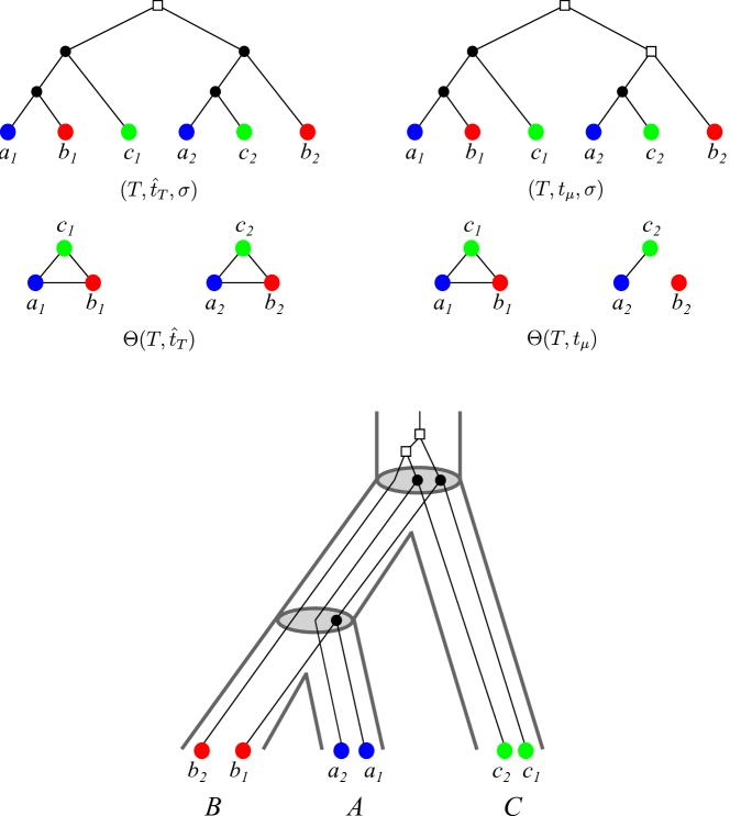
Figure 2: An example for $\Theta(T,t_{\mu})\subset\Theta(T,{\widehat{t}_{T}})$. Top Left: A gene tree $(T,\sigma)$ with extremal event labeling ${\widehat{t}_{T}}$, the corresponding orthology relation $\Theta(T,{\widehat{t}_{T}})$ and map $\sigma(a_{i})=A$, $\sigma(b_{i})=B$ and $\sigma(c_{i})=C$, $i=1,2$. Here we obtain $AB|C,AC|B\in\mathcal{S}(T,{\widehat{t}_{T}},\sigma)$ as conflicting species triples, making $\mathcal{S}(T,{\widehat{t}_{T}},\sigma)$ incompatible. Top Right and Bottom: The same tree $(T,\sigma)$ with another event labeling $t_{\mu}$ defined by the reconciliation map $\mu$ from $(T,\sigma)$ to the (tube-like) species tree $S$ as shown at the bottom. The map $\mu$ is given implicitly by drawing $T$ into $S$. The corresponding orthology relation $\Theta(T,t_{\mu})$ is shown below $(T,t_{\mu},\sigma)$. Clearly, since $\mu$ exists, $\mathcal{S}(T,t_{\mu},\sigma)=\{AB|C\}$ is compatible (cf. Prop. 1).

The event labeling $t$ on $T$ defines the orthology relation:

Definition 5.

(Fitch, 2000) Two distinct leaves $x,y\in L(T)$ are orthologs (w.r.t. $t$) if $t(\operatorname{lca}_{T}(x,y))=\newmoon$; they are paralogs if $t(\operatorname{lca}_{T}(x,y))=\square$.

For completeness, we note that $t(\operatorname{lca}_{T}(x,y))=\odot$ if and only $x=y$, and $0_{T}$ is never the $\operatorname{lca}$ of any of pair of leaves since the planted root $0_{T}$ has degree $1$ by construction. We write $\Theta(T,t)$ for the orthology relation obtained from $(T,t)$, i.e., the set of all unordered pairs $\{x,y\}$ of orthologous genes in $L(T)$. For convenience we will not distinguish between the irreflexive, symmetric binary relation $\Theta(T,t)$ and the graph with vertex set $L(T)$ and edge set $\Theta(T,t)$. Naturally, we say that an arbitrary relation $\Theta$ is an orthology relation if there is an event-labeled phylogenetic tree $(T,t)$ such that $\Theta=\Theta(T,t)$. It is important to note that the orthology relation $\Theta$ explicitly depends on the event labeling. Analogously, one can also define the paralogy relation $\overline{\Theta}$ by $t(\operatorname{lca}_{T}(x,y))=\square$. Both orthology and paralogy are irreflexive and symmetric but not transitive, see Fig. 3. We note that orthology $\Theta$ and paralogy $\overline{\Theta}$ are complementary in the graph-theoretical sense, i.e., $\{x,y\}$ is contained in exactly one of $\Theta$ or $\overline{\Theta}$.

Figure 3: Orthology and paralogy relations are symmetric but not transitive. In this evolutionary scenario with two speciations ($\newmoon$) and two duplications ($\square$), the genes $a_{1}$ and $b_{2}$ are both orthologs of $c_{1}$ but not of each other. The leaves of the gene tree on the l.h.s. are colored corresponding to the three species $A$, $B$, and $C$. The orthology graph $\Theta$ and its complement, the paralogy graph $\overline{\Theta}$, are shown on the r.h.s.

Based on the work of Böcker and Dress (1998) it has been shown by Hellmuth et al. (2013) that valid orthology relations are exactly the cographs:

Proposition 2.

An irreflexive, symmetric relation $\Theta$ on $L$ is an orthology relation if and only if it is a cograph. In this case, every cotree $T$ of $\Theta$ with an event labeling $t$ assigning $\newmoon$ to join operations and $\square$ to disjoint union operations satisfies $\Theta=\Theta(T,t)$.

There is a unique discriminating cotree $(T_{\Theta},t_{\Theta})$ for an orthology relation $\Theta$, which is obtained from every other (non-discriminating) cotree $(T,t)$ for $\Theta$ by contracting the inner edges $uv$ of $T$ if and only if $t(u)=t(v)$ (Böcker and Dress, 1998; Hellmuth et al., 2013).

It is natural then to ask under which conditions a given orthology relation $\Theta$ is consistent with a leaf-labeled tree $(T,\sigma)$ in the sense that there is a reconcilation map $\mu$ from $(T,\sigma)$ to some species tree such that $\Theta=\Theta(T,t_{\mu})$. We first consider the special case $T=T_{\Theta}$. As shown by Hellmuth and Wieseke (2016), it is possible to obtain the set of informative triples $\mathcal{S}(T_{\Theta},t_{\Theta},\sigma)$ directly from $\Theta$ using the following rule:
$\sigma(a)\sigma(b)|\sigma(c)\in\mathcal{S}(T,t,\sigma)$ if and only if $\sigma(a),\sigma(b)$, and $\sigma(c)$ are pairwise different species and either

1. $(a,c),(b,c)\in\Theta$ and $(a,b)\not\in\Theta$ or

2. $(a,c),(b,c),(a,b)\in\Theta$ and there is a vertex $d\neq a,b,c$ with $(c,d)\in\Theta$ and $(a,d),(b,d)\notin\Theta$.

Theorem 1.

Let $\Theta$ be a cograph with vertex set $L$ and associated cotree $(T_{\Theta},t_{\Theta})$ with leaf set $L$ and let $\sigma$ be a leaf coloring. Then there exists a reconciliation map $\mu$ from $(T_{\Theta},t_{\Theta},\sigma)$ to some species tree $S$ if and only if (i) $\mathcal{S}(T_{\Theta},t_{\Theta},\sigma)$ is compatible and (ii) the cograph $(\Theta,\sigma)$ is properly colored, i.e., for all $xy\in E(\Theta)$ we have $\sigma(x)\neq\sigma(y)$.

Proof.

By Proposition 1, it is necessary and sufficient that (i) the set of informative triples is compatible and (ii) the event map $t_{\Theta}$ is well-formed. Since $t_{\Theta}$ is the event labeling of the co-tree, Condition (ii) amounts to requiring that the leaf set $L(T(v_{i}))$ have pairwise disjoint sets of colors $\sigma(L(T(v_{i})))$ for all children $v_{i}\in\mathsf{child}(u)$ of every join node $u$. Since the join $\Theta_{i}\operatorname{\Join}\Theta_{j}$ of the two cographs associated with $T(v_{i})$ and $T(v_{j})$ introduces an edge $xy$ for all $x\in L(T(v_{i}))$ and all $y\in L(T(v_{j}))$, the resulting graph can only be properly colored if $\sigma(L(T(v_{i})))\cap\sigma(L(T(v_{j})))=\emptyset$. On the other hand, every edge in $\Theta$ is the result of a join operation, thus $(\Theta,\sigma)$ can only be well-colored if joins only appear between induced subgraphs with disjoint color sets. Thus $t_{\Theta}$ is well-formed if and only if $\sigma$ is a proper vertex coloring for $\Theta$. ∎

Under the assumption that a reconciliation map $\mu$ exists for $(T,\sigma)$ to some species tree, the next results shows that the orthology relation $\Theta(T,t_{\mu})$ is always a subgraph of the orthology relation $\Theta(T,{\widehat{t}_{T}})$ implied by $(T,\sigma)$ and its extremal labeling ${\widehat{t}_{T}}$.

Lemma 4.

Let $(T,\sigma)$ be a leaf-labeled tree and $\mu$ a reconciliation map from $(T,\sigma)$ to some species tree $S$. Then $\Theta(T,t_{\mu})\subseteq\Theta(T,{\widehat{t}_{T}})$.

Proof.

Let $u=\operatorname{lca}_{T}(x,y)$ and suppose $xy\in\Theta(T,t_{\mu})$. Then, $t_{\mu}(u)=\newmoon$ by definition of $\Theta(T,t_{\mu})$, i.e., $\mu(u)\in V^{0}(S)$. Therefore, Lemma 2 implies $\sigma(L(T(v)))\cap\sigma(L(T(v^{\prime})))=\emptyset$ for all $v,v^{\prime}\in\mathsf{child}_{T}(u)$. Hence, ${\widehat{t}_{T}}(u)=\newmoon$ by definition of the extremal event labeling and thus $xy\in\Theta(T,{\widehat{t}_{T}})$. ∎∎

The converse of Lemma 4 is generally not true, see Fig. 2 for an example. For later reference, we note the following result which is an immediate consequence of Lemma 4 due to fact that orthology and paralogy relation are complementary.

Corollary 1.

Let $(T,\sigma)$ be a leaf-labeled tree and $\mu$ a reconciliation map from $(T,\sigma)$ to some species tree $S$. Then $\overline{\Theta}(T,{\widehat{t}_{T}})\subseteq\overline{\Theta}(T,t_{\mu})$.

Lemma 4, in particular, implies that none of the labelings $t_{\mu}$ (provided by any reconciliation map $\mu$) can yield more speciation events in $T$, than the extremal labeling ${\widehat{t}_{T}}$. Moreover, it is easy to see that $t_{\mu}(v)=\newmoon$ always implies ${\widehat{t}_{T}}(v)=\newmoon$, while ${\widehat{t}_{T}}(v)=\square$ implies $t_{\mu}(v)=\square$.

We briefly compare the formalism introduced here with the literatur on maximum parsimony reconciliations. There, one considers reconciliation maps $\eta:V(T)\to V(S)$ that map duplication events in $T$ also to vertices of $S$. The mapping $\eta$ is then interpreted in such a way that the duplication event $u$ took place along an edge in $S$ that is ancestral to $\eta(u)$. The map $\eta$ in this setting does not completely determine the event labeling. The last common ancestor map

$$\widehat{\eta}(v):=\operatorname{lca}_{S}(\sigma(L(T(v))))\,.$$ (2)

corresponds to one of the “most parsimonious reconciliations” (Górecki and Tiuryn, 2006; Doyon et al., 2009) and can be obtained in polynomial time. A closely related reconciliation map can be defined in our setting. The LCA-reconciliation map introduced by Hellmuth (2017) satisfies the additional axiom

(LCA)

$\mu(u)=v\operatorname{lca}_{S}(\sigma(L(T(u))))\in E(S)$ for all $u\in V(T)$ with $t(u)=\square$, where $v$ denotes the unique parent of $\operatorname{lca}_{S}(\sigma(L(T(u))))\in V(S)$ in $S$.

The Axiom (LCA) is the analog of Equ.(2) for duplication vertices in $T$, which in our formalism are necessarily mapped to edges. For speciation events, the corresponding condition is expressed by (R3.i). Hellmuth (2017) showed that the existence of a reconciliation map from $(T,t,\sigma)$ implies also the existence of an LCA-reconciliation map. Fig. 2 shows that an LCA-reconciliation map does not necessarily have ${\widehat{t}_{T}}$ as its event labeling. Even if $t_{\mu}={\widehat{t}_{T}}$, then $\mu$ is not necessarily an LCA-reconciliation map, see Fig. 4.

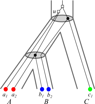
Figure 4: Reconciliation map $\mu$ from $(T,\sigma)$ to the (tube-like) species tree $S$. The map $\mu$ is given implicitly by drawing $(T,\sigma)$ into $S$. The map $\mu$ is not an LCA-reconciliation map since $\mu(u)$ does not map $u$ to the edge $v\operatorname{lca}_{S}(A,B)\in E(S)$ where $v$ denotes the unique parent of $\operatorname{lca}_{S}(A,B)$ in $S$. However, $t_{\mu}$ and the extremal map ${\widehat{t}_{T}}$ coincide.

4 Orthology and Reciprocal Best Matches

In this section, we further clarify the relationship between the orthology relation and (reciprocal) best matches. As a main result, we find that the reciprocal best match graph contains any possible orthology relation.

Lemma 1.

If $(T,\sigma)$ with leaf set $L$ explains the RBMG $(G,\sigma)$ and ${\widehat{t}_{T}}$ is the extremal event labeling of $(T,\sigma)$, then $\Theta(T,{\widehat{t}_{T}})$ is a subgraph of the RBMG $G(T,\sigma)$.

Proof.

Consider a vertex $u\in V^{0}(T)$ with $\mathsf{child}(u)=\{u_{1},\dots,u_{k}\}$. If ${\widehat{t}_{T}}(u)=\square$, then none of the edges $xy$ in $G$ with $x\in L(T(u_{i}))$ and $y\in L(T(u_{j}))$, $1\leq i<j\leq k$ is contained in $\Theta(T,{\widehat{t}_{T}})$.
Now suppose ${\widehat{t}_{T}}(u)=\newmoon$. For $x\in L(T(u_{i}))$ and $y\in L(T(u_{j}))$ with $1\leq i<j\leq k$, we have $xy\in\Theta(T,{\widehat{t}_{T}})$ and, by construction of ${\widehat{t}_{T}}$, $\sigma(x)\neq\sigma(y)$. In particular, ${\widehat{t}_{T}}(u)=\newmoon$ implies that all distinct children $u_{i},u_{j}\in\mathsf{child}(u)$ satisfy $\sigma(L(T(u_{i})))\cap\sigma(L(T(u_{j})))=\emptyset$. Thus, $\operatorname{lca}_{T}(x,y)=u\preceq_{T}\operatorname{lca}_{T}(x^{\prime},y)$ for all $x^{\prime}\neq x$ with $\sigma(x^{\prime})=\sigma(x)$ and $\operatorname{lca}_{T}(x,y)=u\preceq_{T}\operatorname{lca}_{T}(x,y^{\prime})$ for all $y^{\prime}\neq y$ with $\sigma(y^{\prime})=\sigma(y)$, i.e., $x$ and $y$ are reciprocal best matches. Hence, $xy\in E(G)$ and thus $\Theta(T,{\widehat{t}_{T}})\subseteq G(T,\sigma)$. ∎∎

Lemma 4 and 1 immediately imply

Theorem 1.

Let $T$ and $S$ be planted trees, $\sigma:L(T)\to L(S)$ a surjective map, and $\mu$ a reconciliation map from $(T,\sigma)$ to $S$. If $xy\in\Theta(T,t_{\mu})$, then $x$ and $y$ are reciprocal best matches in $(T,\sigma)$.

Observation 1.

Reciprocal best matches therefore cannot produce false negative orthology assignments as long as the evolution of a gene family proceeds via duplications, losses, and speciations only.

The “false positive” edges in the RBMG compared to the orthology relation are the consequence of a particular class of duplication events:

Theorem 2.

Let $(T,t,\sigma)$ be a leaf- and event-labeled gene tree, $G(T,\sigma)$ and $\Theta(T,t)$ its corresponding RBMG and orthology relation, respectively. Moreover, let $a,b\in L(T)$, $v\coloneqq\operatorname{lca}_{T}(a,b)$, and $v_{a},v_{b}\in\mathsf{child}_{T}(v)$ such that $a\preceq v_{a}\prec v$, $b\preceq v_{b}\prec v$. Then, $ab\in E(G(T,\sigma))\setminus E(\Theta(T,t))$ if and only if $t(v)=\square$ and $\sigma(a),\sigma(b)\in\sigma(L(T(v_{a})))\mathbin{\triangle}\sigma(L(T(v_{b})))$, where “$\mathbin{\triangle}$” denotes the usual symmetric set difference.

Proof.

Suppose first $ab\in E(G(T,\sigma))\setminus E(\Theta(T,t))$. By definition of $\Theta(T,t)$, we immediately find $t(v)=\square$. Since $ab\in E(G(T,\sigma))$, i.e., $a$ and $b$ are reciprocal best matches, it must hold $v\preceq_{T}\operatorname{lca}_{T}(a,b^{\prime})$ for any $b^{\prime}$ of color $\sigma(b)$. Hence, $\sigma(b)\notin\sigma(L(T(v_{a})))$. Analogously, we conclude $\sigma(a)\notin\sigma(L(T(v_{b})))$ and thus, $\sigma(a),\sigma(b)\in\sigma(L(T(v_{a})))\mathbin{\triangle}\sigma(L(T(v_{b})))$.

Conversely, assume $t(v)=\square$ and $\sigma(a),\sigma(b)\in\sigma(L(T(v_{b})))\mathbin{\triangle}\sigma(L(T(v_{a})))$. Since $t(v)=\square$, $a$ and $b$ cannot be orthologs, i.e., $ab\notin E(\Theta(T,t))$. Moreover, $\sigma(a)\in\sigma(L(T(v_{b})))\mathbin{\triangle}\sigma(L(T(v_{a})))$ in particular implies $\sigma(a)\notin\sigma(L(T(v_{b})))$ and therefore, $v\preceq_{T}\operatorname{lca}_{T}(a,b^{\prime})$ for any $b^{\prime}$ with $\sigma(b^{\prime})=\sigma(b)$. Hence, $b$ is a best match for $a$ in species $\sigma(b)$. One similarly concludes that $a$ is a best match for $b$. Hence, $a$ and $b$ are reciprocal best matches, which concludes the proof. ∎∎

In practical application we usually do not know the event-labeled gene tree. It is possible, however, to compute the reciprocal best matches directly from sequence data. Therefore, it is of interest to investigate the relationship of reciprocal best match graphs and orthology relations.

Definition 1.

(Geiß et al., 2019b) A tree $(T,\sigma)$ is least resolved (w.r.t. the RBMG $G(T,\sigma)$ that it explains) if the contraction of any inner edge $e\in E(T)$ implies $G(T_{e},\sigma)\neq G(T,\sigma)$.

Since $G(T,\sigma)$ is completely determined by $(T,\sigma)$ we can drop the reference to $G(T,\sigma)$ and often simply speak about a “least resolved tree”.

Lemma 2.

Let $(G,\sigma)$ be an RBMG that is explained by $(T,\sigma)$. If $(T,\sigma)$ is least resolved w.r.t. $(G,\sigma)$, then every inner edge $e=uv\in E(T)$ satisfies $\sigma(L(T(v)))\cap\sigma(L(T(u))\setminus L(T(v)))\neq\emptyset$.

Proof.

For contraposition, assume that there is an inner edge $e=uv\in E(T)$ with $\sigma(L(T(v)))\cap\sigma(L(T(u))\setminus L(T(v)))=\emptyset$. Hence, for all $x\in L(T(v))$ and $y\in L(T(u))\setminus L(T(v))$ we have $\operatorname{lca}_{T}(x,y)=u$ and $\sigma(x)=X\neq\sigma(y)=Y$. It is easy to see that all such $x$ and $y$ form a reciprocal best match and thus, $xy\in E(G)$. Clearly, $x$ and $y$ form also reciprocal best match in $(T_{e},\sigma)$ and thus, each edge $xy\in E(G)$ with $x\in L(T(v))$ and $y\in L(T(u))\setminus L(T(v))$ is contained in $G(T_{e},\sigma)$. Since we have not changed the relative ordering of the $\operatorname{lca}^{\prime}s$ of the remaining vertices, all edges in $E(G)$ are contained in $G(T_{e},\sigma)$. ∎∎

The converse of Lemma 2 is not necessarily true. As an example, consider an inner edge $e=uv\in E(T)$ with $\sigma(L(T(u)))=\sigma(L(T(v)))=\{c\}$. It is easy to see that $e$ can be contracted.

Lemma 2 implies that if $(T,\sigma)$ is least resolved w.r.t. $G(T,\sigma)$ and $u\in V^{0}(T)$ such that $u$ is incident to some other inner vertex $v\in\mathsf{child}(u)$, then there is a child $v^{\prime}\neq v$ of $u$ which satisfies $\sigma(L(T(v^{\prime})))\cap\sigma(L(T(v)))\neq\emptyset$. By construction of ${\widehat{t}_{T}}$ we have ${\widehat{t}_{T}}(u)=\square$. The latter observation also implies the following:

Corollary 1.

Suppose that $(T,\sigma)$ is least resolved w.r.t. $G(T,\sigma)$ and let ${\widehat{t}_{T}}$ be the extremal event labeling for $(T,\sigma)$. Then ${\widehat{t}_{T}}(u)=\newmoon$ if and only if all children of $u$ are leaves that are from pairwise distinct species.

Lemma 3.

Let $(T,\sigma)$ be some least resolved tree (w.r.t. some RBMG) with extremal event map ${\widehat{t}_{T}}$ and let $S(W,F)$ be a species tree with $L(S)=\sigma(L(T))$. Then there is a reconciliation map $\mu:V(T)\to V(S)\cup E(S)$ such that $t_{\mu}={\widehat{t}_{T}}$.

Proof.

By Cor. 1, every inner vertex $u$ with ${\widehat{t}_{T}}(u)=\newmoon$ is only incident to leaves from pairwise distinct species. However, this implies that the set of informative species triples $\mathcal{S}(T,{\widehat{t}_{T}},\sigma)$ is empty, and thus, compatible. Hence, Proposition 1 implies that there is a reconciliation map $\mu$ from $(T,{\widehat{t}_{T}},\sigma)$ to any species tree $S$, defined by $\mu(0_{T})=0_{S}$, $\mu(v)=0_{S}\rho_{S}$ for every inner vertex $v\in V^{0}(T)$ that is incident to another inner vertex in $T$, and $\mu(v)=x=\operatorname{lca}_{S}(\sigma(L(T(v))))$ for any inner vertex $v$ that is only incident to leaves that are from pairwise distinct species, and $\mu(v)=\sigma(v)$ for all leaves of $T$. By construction of $\mu$, we have ${\widehat{t}_{T}}(u)=t_{\mu}(u)$ with $t_{\mu}(u)$ specified by Def. 2 for all $u\in V(T)$. ∎∎

Corollary 2.

Let $(T,\sigma)$ be a least resolved tree explaining a co-RBMG $(G,\sigma)$. Then $(\Theta(T,{\widehat{t}_{T}}),\sigma)$ is a disjoint union of cliques.

Proof.

By Cor. 1 all children of a speciation node $u$ w.r.t. ${\widehat{t}_{T}}$ are leaves from pairwise distinct species. Thus the leaves $L(T(u))$ form a complete subgraph in $(\Theta(T,{\widehat{t}_{T}}),\sigma)$. On the other hand, no ancestor of $u$ is a speciation, i.e., there is no edge $ab$ with $a\in L(T(u))$ and $b\notin L(T(u))$. Thus $(\Theta(T,{\widehat{t}_{T}}),\sigma)$ is a disjoint union of the cliques formed by the $L(T(u))$ with ${\widehat{t}_{T}}(u)=\newmoon$ possibly together with isolated vertices that are not children of any speciation node in $(T,{\widehat{t}_{T}})$. ∎

Suppose that we know the orthology relation $\Theta(T,{\widehat{t}_{T}})$ that is obtained from a least resolved tree $(T,\sigma)$ that explains the RBMG $(G,\sigma)$. Lemma 3 implies that there is always a reconciliation map $\mu$ from $(T,\sigma)$ to any species tree $S$ with $L(S)=\sigma(L(T))$ such that ${\widehat{t}_{T}}$ is determined by $\mu$ as in Def. 2. Now we can apply Theorem 1 to conclude that all orthologous pairs in $\Theta(T,{\widehat{t}_{T}})$ are reciprocal best matches. In other words, all complete subgraphs of $\Theta(T,{\widehat{t}_{T}})$ are also induced subgraphs of the underlying RBMG $(G,\sigma)$. Hence, $\Theta(T,{\widehat{t}_{T}})$ is obtained from $(G,\sigma)$ by removing edges such that the resulting graph is the disjoint union of cliques, see the top-right tree in Fig. 5 for an example. However, Fig. 5 also shows that many edges have to be removed to obtain $\Theta(T,{\widehat{t}_{T}})$.

This observation establishes the precise relationship of orthology detection and clustering, since (graph) clustering can be interpreted as the graph editing problem for disjoint unions of complete graphs (Böcker et al., 2011). In many orthology prediction tools, such as e.g. OMA (Roth et al., 2008), orthologs are summarized as clusters of orthologous groups (COGs) (Tatusov et al., 1997) that are obtained from reciprocal best matches.

The results above show that the RBMGs contain the orthology relation. Equivalently, RBMGs imply constraints on the event labeling. We also observe that the RBMGs cannot provide conclusive evidence regarding edges that must correspond to orthologous pairs. In the following sections we consider the constraints implied by the detailed structure of RBMGs or BMGs in more detail.

5 Classification of RBMGs

The structure of RBMGs has been studied in extensive detail by Geiß et al. (2019b). Although we do not have an algorithmically useful complete characterization of RBMGs, there are partial results that can be used to identify different subclasses of RBMGs based on the structure of the connected components of the 3-colored subgraphs (Geiß et al., 2019b, Thm. 7). Let $\mathscr{C}(G,\sigma)$ be the set of the connected components of the induced subgraphs on three colors of an RBMG $(G,\sigma)$. Then every $(C,\sigma)\in\mathscr{C}(G,\sigma)$ is precisely of one of the three types (Geiß et al., 2019b, Thm. 5):

Type (A)

$(C,\sigma)$ contains a $K_{3}$ on three colors but no induced $P_{4}$.

Type (B)

$(C,\sigma)$ contains an induced $P_{4}$ on three colors whose endpoints have the same color, but no induced cycle $C_{n}$ on $n\geq 5$ vertices.

Type (C)

$(C,\sigma)$ contains an induced cycle $C_{6}$, called hexagon, such that any three consecutive vertices have pairwise distinct colors.

The graphs for which all $(C,\sigma)\in\mathscr{C}(G,\sigma)$ are of Type (A) are exactly the RBMGs that are cographs, or co-RBMGs for short (Geiß et al., 2019b, Thm. 8 and Remark 2). Intuitively, these have a close connection to orthology graphs because orthology graphs are cographs.

Connected components of Type (B) and Type (C), on the other hand, contain induced $P_{4}$s and thus are neither cographs nor connected components of cographs. Obs. 1 implies that RBMGs that contain connected components of Type (B) and Type (C) introduce false positive edges into estimates of the orthology relation. In Section 6 below we will address the question to what extent and how such false-positives edges can be identified. We distinguish here co-RBMGs, (B)-RBMGs, and (C)-RBMGs depending on whether $\mathscr{C}(G,\sigma)$ contains only Type (A) components, at least one Type (B) but not Type (C) component, or at least one Type (C) component.

Co-RBMGs have a convenient structure that can be readily understood in terms of hierarchically colored cographs (hc-cographs) introduced by Geiß et al. (2019b, Section 7).

Definition 1.

An undirected colored graph $(G,\sigma)$ is a hierarchically colored cograph (hc-cograph) if

(K1)

$(G,\sigma)=(K_{1},\sigma)$, i.e., a colored vertex, or

(K2)

$(G,\sigma)=(H_{1},\sigma_{H_{1}})\operatorname{\Join}(H_{2},\sigma_{H_{2}})$ and $\sigma(V(H_{1}))\cap\sigma(V(H_{2}))=\emptyset$, or

(K3)

$(G,\sigma)=(H_{1},\sigma_{H_{1}})\mathbin{\mathchoice{\leavevmode\vtop{\halign{\hfil$\m@th\displaystyle#$\hfil\cr\cup\cr\cdot\crcr}}}{\leavevmode\vtop{\halign{\hfil$\m@th\textstyle#$\hfil\cr\cup\cr\cdot\crcr}}}{\leavevmode\vtop{\halign{\hfil$\m@th\scriptstyle#$\hfil\cr\cup\cr\cdot\crcr}}}{\leavevmode\vtop{\halign{\hfil$\m@th\scriptscriptstyle#$\hfil\cr\cup\cr\cdot\crcr}}}}(H_{2},\sigma_{H_{2}})$ and $\sigma(V(H_{1}))\cap\sigma(V(H_{2}))\in\{\sigma(V(H_{1})),\sigma(V(H_{2}))\}$,

where both $(H_{1},\sigma_{H_{1}})$ and $(H_{2},\sigma_{H_{2}})$ are hc-cographs and $\sigma(x)=\sigma_{H_{i}}(x)$ for any $x\in V(H_{i})$ for $i\in\{1,2\}$.

Not all properly colored cographs are hc-cographs, see e.g. Geiß et al. (2019b) for counterexamples. However, for each cograph $G$, there exists a coloring $\sigma$ (with a sufficient number of colors) such that $(G,\sigma)$ is an hc-cograph.

Proposition 3 (Thm. 9 in (Geiß et al., 2019b)).

A graph $(G,\sigma)$ a co-RBMG if and only if it is an hc-cograph.

Since orthology relations are necessarily cographs we can interpret Proposition 3 as necessary condition for an RBMG to correctly represent orthology.

The recursive construction of $(G,\sigma)$ in Def. 1 also defines a corresponding hc-cotree $(T^{G}_{\emph{hc}},t_{\emph{hc}},\sigma)$ whose leaves are the vertices of $(G,\sigma)$, i.e., the $(K_{1},\sigma)$ appearing in (K1). Each internal node $u$ of $T^{G}_{\emph{hc}}$ corresponds to either a join (K2) or a disjoint union (K3) and is labeled by $t_{\emph{hc}}:V(T^{G}_{\emph{hc}})\setminus L\to\{\square,\newmoon\}$ such that $t_{\emph{hc}}(u)=\newmoon$ if $u$ represents a join, and $t_{\emph{hc}}(u)=\square$ if $u$ corresponds to a disjoint union. Each inner vertex $u$ of $T^{G}_{\emph{hc}}$ represents the induced subgraph $(G,\sigma)[L(T^{G}_{\emph{hc}}(u))]$.

Proposition 4 (Thm. 10 in (Geiß et al., 2019b)).

Every co-RBMG $(G,\sigma)$ is explained by its hc-cotree $(T^{G}_{\emph{hc}},t_{\emph{hc}},\sigma)$.

Now let $(T^{G}_{\emph{hc}},t_{\emph{hc}},\sigma)$ be the hc-cotree of a co-RBMG $(G,\sigma)$. Note, the structure of $T^{G}_{\emph{hc}}$ is solely determined by the hc-cograph structure of $(G,\sigma)$. Somehwat surprisingly, the mathematical structure of the hc-cotree $(T^{G}_{\emph{hc}},t_{\emph{hc}},\sigma)$ and, in particular, its coloring $t_{\emph{hc}}$ has a simple biological interpretation. Consider $\{v^{\prime},v^{\prime\prime}\}=\mathsf{child}(u)$. If $t_{\emph{hc}}(u)=\newmoon$ in the hc-cotree, then $\sigma(L(T^{G}_{\emph{hc}}(v^{\prime})))\cap\sigma(L(T^{G}_{\emph{hc}}(v^{\prime\prime})))=\emptyset$ in agreement with Lemma 2. On the other hand, if $t_{\emph{hc}}(u)=\square$, then (K3) implies $\sigma(L(T^{G}_{\emph{hc}}(v^{\prime})))\cap\sigma(L(T^{G}_{\emph{hc}}(v^{\prime\prime})))\neq\emptyset$, in which case $u$ indeed must be a duplication from the biological point of view (contraposition of Lemma 2).

The hc-cotree $(T^{G}_{\emph{hc}},t_{\emph{hc}},\sigma)$ of $(G,\sigma)$ will in general not be discriminating and it is not necessarily possible to reduce $(T^{G}_{\emph{hc}},t_{\emph{hc}},\sigma)$ to a discriminating hc-cotree $(\widehat{T}^{G}_{\emph{hc}},\widehat{t},\sigma)$ that still explains $(G,\sigma)$. Although it is always possible to contract edges $uv$ of $(T^{G}_{\emph{hc}},t_{\emph{hc}},\sigma)$ with $t_{\emph{hc}}(u)=t_{\emph{hc}}(u)=\newmoon$ (cf. (Geiß et al., 2019b, Cor. 11)), there are examples where edges $uv$ with $t_{\emph{hc}}(u)=t_{\emph{hc}}(u)=\square$ cannot be contracted to obtain a tree that still explains $(G,\sigma)$ (cf. (Geiß et al., 2019b, Fig. 15)). We refer to (Geiß et al., 2019b) for more details and a characterization of edges that are contractable. It is of interest, therefore, to ask whether there are true orthology relations $\Theta$ that are not hc-cographs, or equivalently, when does a discriminating hc-cotree $(\widehat{T},\widehat{t},\sigma)$ that is obtained by edge-contraction from a given hc-cotree $(T^{G}_{\emph{hc}},t_{\emph{hc}},\sigma)$ still explains an RBMG $(G,\sigma)$? To answer this question we provide first

Definition 2.

A tree $(T,t,\sigma)$ contains no losses, if for all $x\in V(T)$ with $t(x)=\square$ we have $\sigma(L(T(v^{\prime})))=\sigma(L(T(v^{\prime\prime})))$ for all $v^{\prime},v^{\prime\prime}\in\mathsf{child}(x)$.

Theorem 1.

Let $(T,\sigma)$ be a leaf-labeled tree such that there is a reconciliation map $\mu$ to some species tree and assume that $(T,t_{\mu},\sigma)$ does not contain losses. Then

1. The RBMG $G(T,\sigma)$ explained by $(T,\sigma)$ equals the colored cograph $(\Theta(T,t_{\mu}),\sigma)$.

2. The unique disciminating cotree $(\widehat{T},\widehat{t},\sigma)$ of $(\Theta(T,t_{\mu}),\sigma)$ explains the RBMG $(G,\sigma)$.

Proof.

To simplify the notation, we set $(G,\sigma)=G(T,\sigma)$ and $(H,\sigma)=(\Theta(T,t_{\mu}),\sigma)$.

We start with proving Statement (1). By Theorem 1, $(H,\sigma)$ is a subgraph of $(G,\sigma)$ and $V(H)=V(G)$, hence it suffices to show that every edge $ab\in E(G)$ is also contained in $E(H)$. Assume, for contradiction, that this is not the case, i.e., $ab\notin E(H)$, and thus $t_{\mu}(x)=\square$ for $x\coloneqq\operatorname{lca}_{T}(a,b)$. Since $(T,t,\sigma)$ has no losses, we have $\sigma(L(T(v^{\prime})))=\sigma(L(T(v^{\prime\prime})))$ for all $v^{\prime},v^{\prime\prime}\in\mathsf{child}(x)$, and thus $a\in L(T(v^{\prime}))$ and $b\in L(T(v^{\prime\prime}))$ for some pair of distinct children $v^{\prime},v^{\prime\prime}\in\mathsf{child}(x)$ of $x$. From $\sigma(L(T(v^{\prime})))=\sigma(L(T(v^{\prime\prime})))$ we know that there is a vertex $a^{\prime}\in L(T(v^{\prime\prime}))$ with $\sigma(a^{\prime})=\sigma(a)$. Thus, $\operatorname{lca}_{T}(a,b)=x\succ_{T}\operatorname{lca}_{T}(a^{\prime},b)$ for some $a^{\prime}\in L(T(v^{\prime\prime}))$, which implies that $ab\notin E(G)$; a contradiction. We conclude that $ab\in E(G)$ if and only if $ab\in E(H)$ and thus $(G,\sigma)=(H,\sigma)$.

Let us now turn to Statement (2). In order to show that $(\widehat{T},\widehat{t},\sigma)$ explains the RBMG $(G,\sigma)$ we first note that, since $(G,\sigma)$ is a cograph by Statement (1), there is a unique discriminating cotree $(\widehat{T},\widehat{t},\sigma)$ for $(G,\sigma)$. Furthermore, $(\widehat{T},\widehat{t},\sigma)$ is obtained from any cotree $(T,t_{\mu},\sigma)$ for $(G,\sigma)$ by contracting all edges $uv$ in $T$ with $t_{\mu}(u)=t_{\mu}(v)$ (Hellmuth et al., 2013). It remains to show that $ab$ is an edge in $(G,\sigma)$ if and only if $ab$ forms a reciprocal best match in $(\widehat{T},\sigma)$.

First consider duplications. Suppose, we have contracted the edge $xv$ with $t_{\mu}(x)=t_{\mu}(v)=\square$. By assumption, for all children $v^{\prime},v^{\prime\prime}$ of $v$ we have $\sigma(L(T(v^{\prime})))=\sigma(L(T(v^{\prime\prime})))$. Moreover, since $\sigma(L(T(v)))$ is the union of species $\sigma(L(T(w))))$ of its children $w$, we have $\sigma(L(T(v)))=\sigma(L(T(v^{\prime})))=\sigma(L(T(v^{\prime\prime})))$. Hence, after contraction of $xv$, the vertices $v^{\prime}$ and $v^{\prime\prime}$ are now children of $x$ and still satisfy $\sigma(L(\widehat{T}(v^{\prime})))=\sigma(L(\widehat{T}(v^{\prime\prime})))$. In particular, $\sigma(L(\widehat{T}(v^{\prime})))=\sigma(L(\widehat{T}(w)))$ for every child $w$ of $x$. By induction on the number of contracted edges, every vertex $x$ in $\widehat{T}$ with $\widehat{t}(x)=\square$ still satisfies $\sigma(L(\widehat{T}(v^{\prime})))=\sigma(L(\widehat{T}(v^{\prime\prime})))$ for all children $v^{\prime},v^{\prime\prime}$ of $x$ in $\widehat{T}$. Thus, the same argument as in the proof of Statement (1) implies that $ab$ cannot be a reciprocal best match in $\widehat{T}$ for all $a\in L(T(v^{\prime}))$ and $b\in L(T(v^{\prime\prime}))$. We also have $\operatorname{lca}_{\widehat{T}}(a,b)=x$ for $a\in L(T(v^{\prime}))$ and $b\in L(T(v^{\prime\prime}))$, and thus $\widehat{t}(\operatorname{lca}_{\widehat{T}}(a,b))=\square$. Since $(\widehat{T},\widehat{t},\sigma)$ is a cotree for the cograph $(G,\sigma)$, $\widehat{t}(\operatorname{lca}_{\widehat{T}}(a,b))=\square$ implies $ab\notin E(G)$. Therefore, $ab\notin E(G)$ unless $a$ and $b$ form a reciprocal best match in $(\widehat{T},\sigma)$. Let us now turn to speciation vertices. Lemma 47 in (Geiß et al., 2019b) states, in particular, that all non-discriminating edges $uv$ with $t_{\mu}(u)=t_{\mu}(v)=\newmoon$ can be contracted to obtain a tree that still explains $(G,\sigma)$. Thus, if $a$ and $b$ are reciprocal best matches in $(\widehat{T},\sigma)$, then $ab\in E(G)$. We conclude, therefore, that $ab\in E(G)$ if and only if $a$ and $b$ are reciprocal best matches in $(\widehat{T},\sigma)$. ∎∎

Prop. 3 shows that if the no loss condition of Def. 2 holds, then $(\Theta(T,t_{\mu}),\sigma)=G(T,\sigma)$ is a co-RBMG, an hc-cograph, and an orthology relation.

The no loss condition of Def. 2 is very restrictive, however, and thus in general is will not be satisfied in real-life data. Theorem 1 shows that orthology relations correspond to properly colored cographs with compatible sets of the informative triples. The characterization of co-RBMGs in (Geiß et al., 2019b), on the other hand, shows that only hc-colorings may appear. Since the requirement that $\sigma$ is a proper coloring already implies disjointness of the color sets for join operations, we can interpret the hc-coloring condition as a condition on duplication vertices. The offending vertices are exactly those for which (i) $t(u)=\square$ and (ii) there are two children $v^{\prime},v^{\prime\prime}\in\mathsf{child}(u)$ such that both $\sigma(L(T(v^{\prime})))\setminus\sigma(L(T(v^{\prime\prime})))\neq\emptyset$ and $\sigma(L(T(v^{\prime\prime})))\setminus\sigma(L(T(v^{\prime})))\neq\emptyset$. In this case, there is a pair of species such that a different “paralog group” (that is, a lineage of genes descending from a duplication) is missing in each of them. Every pair of vertices $a\in L(T(v^{\prime}))$ with $\sigma(a)\notin\sigma(L(T(v^{\prime\prime})))$ and $b\in L(T(v^{\prime\prime}))$ with $\sigma(b)\notin\sigma(L(T(v^{\prime})))$ forms a best match and thus a false positive orthology assignment. Since an RBMG is a cograph only if it is hierarchically colored, the presence of such duplications implies that the RBMG is not a cograph. At least in principle, therefore, it should be possible to identify the false positive edges by means of a suitable cograph-editing approach.

Before closing this section, we briefly return to the existence of reconciliation maps. Since every hc-cograph is a properly colored cograph, Theorem 1 immediately implies

Corollary 1.

Let $\Theta$ be an hc-cograph with vertex set $L$ and associated hc-cotree $(T^{\Theta}_{\emph{hc}},t_{\emph{hc}},\sigma)$ with leaf set $L$. Then there exists a reconciliation map $\mu$ from $(T^{\Theta}_{\emph{hc}},t_{\emph{hc}},\sigma)$ to some species tree $S$ if and only if $\mathcal{S}(T_{\Theta},t_{\Theta},\sigma)$ is compatible.

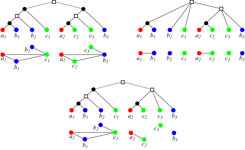
Figure 5: Top Left: A (discriminating) hc-cotree $(T^{G}_{\emph{hc}},t_{\emph{hc}},\sigma)$. Its corresponding hc-cograph $(G,\sigma)=(\Theta(T^{G}_{\emph{hc}},t_{\emph{hc}}),\sigma)$ is drawn below $(T^{G}_{\emph{hc}},t_{\emph{hc}},\sigma)$. In fact, Prop. 3 implies that $(G,\sigma)$ is an RBMG. Top Right: A tree $(T^{*},{\widehat{t}_{T}},\sigma)$ that is least resolved w.r.t. the RBMG $(G,\sigma)$ together with extremal labeling ${\widehat{t}_{T}}$ and the resulting orthology relation $\Theta(T^{*},{\widehat{t}_{T}})$, where $(T^{*},{\widehat{t}_{T}})$ is not discriminating. Below: A tree $(T,{\widehat{t}_{T}},\sigma)$ together with extremal labeling ${\widehat{t}_{T}}$ that explains the RBMG $(G,\sigma)$ but is not least resolved w.r.t. $(G,\sigma)$. The resulting orthology relation $\Theta(T,{\widehat{t}_{T}})$ is drawn below $(T,{\widehat{t}_{T}},\sigma)$.

By Cor. 1, it is not necessarily possible to reconcile a (discriminating) hc-cotree with any species tree. An example is shown in Fig. 5. To be more precise, the hc-cotree $(T^{G}_{\emph{hc}},t_{\emph{hc}},\sigma)$ in Fig. 5 yields the conflicting species triples $AB|C$ and $AC|B$. Hence, Prop. 1 implies that $(T^{G}_{\emph{hc}},t_{\emph{hc}},\sigma)$ cannot be reconciled with any species tree even though $(T^{G}_{\emph{hc}},\sigma)$ explains the RBMG $(G,\sigma)$. One can contract edges of $(T^{G}_{\emph{hc}},\sigma)$ to obtain a least resolved tree $(T^{*},\sigma)$ that still explains $(G,\sigma)$, see Fig. 5 (top right). In agreement with Lemma 3, $\mathcal{S}(T^{*},t_{\mu},\sigma)=\emptyset$ and thus, there is always a reconciliation map $\mu$ from $(T^{*},t_{\mu},\sigma)$ to any species tree $S$ with $L(S)=\sigma(L(T))$. Moreover, in agreement with Theorem 1, all orthologous pairs in $\Theta(T^{*},{\widehat{t}_{T}},\sigma)$ are best matches. Although $(T^{*},\sigma)$ explains $(G,\sigma)$, the two graphs $(G,\sigma)=(\Theta(T^{G}_{\emph{hc}},t),\sigma)$ and $(\Theta(T^{*},{\widehat{t}_{T}}),\sigma)$ are very different. In particular, by Corollary 2, $\Theta(T^{*},{\widehat{t}_{T}})$ is the disjoint union of cliques.

Observation 2.

In general it is not necessary to edit $(G,\sigma)$ to a disjoint union of cliques to obtain a valid orthology relation.

An example is provided by the tree $(T,{\widehat{t}_{T}},\sigma)$ in Fig. 5. Obviously, $\Theta(T,{\widehat{t}_{T}})$ is not the disjoint union of cliques. Moreover, $AB|C$ is the only informative triple displayed by $(T,{\widehat{t}_{T}},\sigma)$ where $A$, $B$, and $C$ correspond to the red, blue and green species, respectively. Prop. 1 implies that $(T,{\widehat{t}_{T}},\sigma)$ can be reconciled with any species tree that displays $AB|C$. In other words, $\Theta(T,{\widehat{t}_{T}})$ is already “biologically feasible” and there is no need to remove further edges from $\Theta(T,{\widehat{t}_{T}})$.

6 Non-Orthologous Reciprocal Best Matches

In this section we investigate to what extent false positive orthology assignments in the reciprocal best match graph can be identified. Since the orthology relation $\Theta$ must be a cograph, it is natural to consider the smallest obstructions, i.e., induced $P_{4}$s in more detail. First we note that every induced $P_{4}$ in an RBMG contains either three or four distinct colors (Geiß et al., 2019b, Sect. E). Each $P_{4}$ in an RBMG $(G,\sigma)$ spans an induced subgraph of every BMG $(\mathaccent 382{G},\sigma)$ that contains $(G,\sigma)$ as its symmetric part. These these induced subgraphs of a BMG $(\mathaccent 382{G},\sigma)$ with four vertices are known as quartets. With respect to a fixed BMG, every induced $P_{4}$ belongs to one of three distinct types which are defined in terms of its coloring and the quartet in which it resides. An induced $P_{4}$ with edges $ab$, $bc$, and $cd$ is denoted by $\langle abcd\rangle$ or, equivalently, $\langle dcba\rangle$.

Definition 1.

Let $(\mathaccent 382{G},\sigma)$ be a BMG explained by the tree $(T,\sigma)$, with symmetric part $(G,\sigma)$ and let $Q\coloneqq\{x,x^{\prime},y,z\}\subseteq L(T)$ with $\sigma(x)=\sigma(x^{\prime})$ and pairwise distinct colors $\sigma(x)$, $\sigma(y)$, and $\sigma(z)$. The set $Q$, resp., the induced subgraph $(\mathaccent 382{G}_{|Q},\sigma_{|Q})$ is

• a good quartet if (i) $\langle xyzx^{\prime}\rangle$ is an induced $P_{4}$ in $(G,\sigma)$ and (ii) $(x,z),(x^{\prime},y)\in E(\mathaccent 382{G})$ and $(z,x),(y,x^{\prime})\notin E(\mathaccent 382{G})$,

• a bad quartet if (i) $\langle xyzx^{\prime}\rangle$ is an induced $P_{4}$ in $(G,\sigma)$ and (ii) $(z,x),(y,x^{\prime})\in E(\mathaccent 382{G})$ and $(x,z),(x^{\prime},y)\notin E(\mathaccent 382{G})$, and

• an ugly quartet if $\langle xyx^{\prime}z\rangle$ is an induced $P_{4}$ in $(G,\sigma)$.

If $Q$ is a good, bad, or ugly quartet we will refer to the underlying induced $P_{4}$ as a good, bad, or ugly quartet, respectively. Lemma 32 of (Geiß et al., 2019b) states that every quartet $Q$ in an RBMG $(G,\sigma)$ that is contained in a BMG $(\mathaccent 382{G},\sigma)$ is either good, bad, or ugly. An example of an RBMG containing good, bad, and ugly quartets is shown in Fig. 6. Note that good, bad, and ugly quartets cannot appear in RBMGs of Type (A). These are cographs and thus by definition do not contain induced $P_{4}$s.

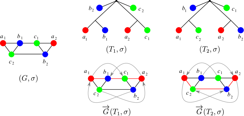
Figure 6: The 3-RBMG $(G,\sigma)$ is explained by two trees $(T_{1},\sigma)$ and $(T_{2},\sigma)$. These induce distinct BMGs $\mathaccent 382{G}(T_{1},\sigma)$ and $\mathaccent 382{G}(T_{2},\sigma)$. In $\mathaccent 382{G}(T_{1},\sigma)$, $P^{1}=\langle a_{1}b_{1}c_{1}a_{2}\rangle$ defines a good quartet, while $P^{2}=\langle a_{1}c_{2}b_{2}a_{2}\rangle$ induces a bad quartet. In $\mathaccent 382{G}(T_{2},\sigma)$ the situation is reversed. The good quartets in $\mathaccent 382{G}(T_{1},\sigma)$ and $\mathaccent 382{G}(T_{2},\sigma)$ are indicated by red edges. The induced paths $\langle a_{1}b_{1}c_{1}b_{2}\rangle$ and $\langle a_{2}c_{1}b_{1}c_{2}\rangle$ are examples of ugly quartets. Figure reused from (Geiß et al., 2019b), ©Springer

The location of good quartets (in contrast to bad and ugly quartets) turns out to be strictly constrained. This fact can be used to show that the “middle” edge of any good quartet must be a false positive orthology assignment:

Lemma 1.

Let $(T,\sigma)$ be some leaf-labeled tree and $\widehat{t}_{T}$ the extremal event labeling for $(T,\sigma)$. If $\langle xyzx^{\prime}\rangle$ is a good quartet in the BMG $\mathaccent 382{G}(T,\sigma)$, then ${\widehat{t}_{T}}(v)=\square$ for $v\coloneqq\operatorname{lca}(x,x^{\prime},y,z)$.

Proof.

Lemma 36 of Geiß et al. (2019b) implies that for a good quartet $\langle xyzx^{\prime}\rangle$ in $\mathaccent 382{G}(T,\sigma)$ with $v\coloneqq\operatorname{lca}(x,x^{\prime},y,z)$ there are two distinct children $v_{1},v_{2}\in\mathsf{child}(v)$ such that $x,y\preceq_{T}v_{1}$ and $x^{\prime},z\preceq_{T}v_{2}$. Thus, in particular, $v_{1}$ and $v_{2}$ must be inner vertices in $(T,\sigma)$. Since $\sigma(x)=\sigma(x^{\prime})$ by definition of a good quartet, we have $\sigma(L(T(v_{1})))\cap\sigma(L(T(v_{2})))\neq\emptyset$. Hence, ${\widehat{t}_{T}}(v)\neq\newmoon$ by definition of ${\widehat{t}_{T}}$ (cf. Definition 4). ∎∎

As an immediate consequence of Lemma 1 and Cor. 1, an analogous statement is true for event labelings $t_{\mu}$ for a given reconciliation map:

Corollary 1.

Let $T$ and $S$ be planted trees, $\sigma:L(T)\to L(S)$ a surjective map, and $\mu$ a reconciliation map from $(T,\sigma)$ to $S$. If $\langle xyzx^{\prime}\rangle$ is a good quartet in the BMG $\mathaccent 382{G}(T,\sigma)$, then $t_{\mu}(v)=\square$ for $v\coloneqq\operatorname{lca}(x,x^{\prime},y,z)$.

Given an RBMG $(G,\sigma)$ that contains a good quartet $\langle xyzx^{\prime}\rangle$ (w.r.t. to the underlying BMG $(\mathaccent 382{G},\sigma)$), the edge $yz$ therefore always corresponds to a false positive orthology assignment, i.e., it is not contained in the true orthology relation $\Theta$.

Not all false positives can be identified in this way from good quartets, however. The RBMG $G(T_{1},\sigma)$ in Fig. 7, for instance, contains only one good quartet, that is $\langle a_{1}c_{2}b_{2}a_{2}\rangle$. After removal of the false positive edge $c_{2}b_{2}$, the remaining undirected graph still contains the bad quartet $\langle a_{1}b_{1}c_{1}a_{2}\rangle$, hence, in particular, it still contains an induced $P_{4}$ and is, therefore, not an orthology relation.

Neither bad nor ugly quartets can be used to unambiguously identify false positive edges. For an example, consider Fig. 7. The two 3-RBMGs $G(T_{1},\sigma)$ and $G(T_{2},\sigma)$ both contain the bad quartet $\langle a_{1}b_{1}c_{1}a_{2}\rangle$. As a consequence of Lemma 2, neither the root of $T_{1}$ nor the root of $T_{2}$ can be labeled by a speciation event. Hence, as $a_{1},b_{1},c_{1},a_{2}$ reside all in different subtrees below the root of $T_{1}$, all edges $a_{1}b_{1},b_{1}c_{1},c_{1}a_{2}$ in $G(T_{1},\sigma)$ correspond to false positive orthology assignments. On the other hand, the vertices $b_{1}$ and $c_{1}$ reside within the same 2-colored subtree below the root of $T_{2}$ and are incident to the same parent in $T_{2}$. Therefore, one easily checks that there exist reconciliation scenarios where $b_{1}$ and $c_{1}$ are orthologous, hence the edge $b_{1}c_{1}$ must indeed be contained in the orthology relation. Similarly, $\langle a_{1}b_{1}c_{1}b_{2}\rangle$ and $\langle a_{1}b_{1}a_{3}c_{2}\rangle$ are ugly quartets in $G(T_{1},\sigma)$ and $G(T_{2},\sigma)$, respectively. By the same argumentation as before, the edges $a_{1}b_{1}$, $b_{1}c_{1}$, and $c_{1}b_{2}$ are false positives in $G(T_{1},\sigma)$. For $(T_{2},\sigma)$, however, there exist reconciliation scenarios, where $a_{3}$ and $c_{2}$ are orthologs.

Figure 7: Not all false positive orthology assignments can be identified using good quartets. Conversely, bad and ugly quartets do not unambiguously identifiy false positive edges. See the text below Cor. 1 for explanation.

Cor. 9 of Geiß et al. (2019b), finally, implies that every (B)-RBMG and every (C)-RBMG contains at least one good quartet. In particular, therefore, there is at least one false positive orthology assignment that can be identified with the help of good quartets. We shall see in Section 7.2, using simulated data, that in practice the overwhelming majority of false positive orthology assignments is already identified by good quartets.

From a theoretical point of view it is interesting nevertheless that it is possible to identify even more false positive orthology assignments starting from Lemma 2. It implies that $t(\operatorname{lca}(x,y))=\square$ whenever $x$ and $y$ are located in two distinct leaf sets defined for the the same connected component of an induced 3-RBMG of Type (B) or (C). Details can be found in (Geiß et al., 2019b, Lemma 25) and the Supplemental Material. At least in our simulation data scenarios of this type that are not covered already by a good quartet seem to be exceedingly rare, and hence of little practical relevance.

7 Simulations

Although the edges in the RMBG cannot identify orthologous pairs with certainty (as a consequence to Lemma 3), there is a close resemblance in practice, i.e., for empirically determined scenarios. In order to explore this connection in more detail, we consider simulated evolutionary scenarios $(T,S,\mu)$. These uniquely determine both the (reciprocal) best match graph $\mathaccent 382{G}(T,\sigma)$ and $G(T,\sigma)$, resp., and the orthology graph $\Theta$, thus allowing a direct comparison of these graphs. Since we only analyze scenarios $(T,S,\mu)$, we did not use simulations tools such as ALF (Dalquén et al., 2011) that are designed to simulate sequence data.

7.1 Simulation Methods

In order to simulate evolutionary scenarios $(T,S,\mu)$ we employ a stepwise procedure:

• Construction of the species tree $S$. We regard $S$ as an ultrametric tree, i.e., its branch lengths are interpreted as real-time. Given a user-defined number of species $N$ we generate $S$ under the innovations model as described by Keller-Schmidt and Klemm (2012). The binary trees generated by this model have similar depth and imbalances as those of real phylogenetic trees from databases.

• Construction of the true gene tree $\widetilde{T}$. Traversing the species tree $S$ top-down, one gene tree $\widetilde{T}$ is generated with user-defined rates $r_{D}$ for duplications, $r_{L}$ for losses, and $r_{H}$ for horizontal transfer events. The number of events along each edge of the species tree, of each type of event, is drawn from a Poisson distribution with parameter $\lambda=\ell r_{e}$, where $\ell$ is the length of the edge $e$ and $r_{e}$ is the rate of the event type. Duplication and horizontal transfer events duplicate an active lineage and occur only inside edges of $S$. For duplications, both offspring lineages remain inside the same edge of the species tree as the parental gene. In contrast, one of the two offsprings of an HGT event is transferred to another, randomly selected, branch of the species tree at the same time. At speciation nodes all branches of the gene tree are copied into each offspring. Loss events terminate branches of $\widetilde{T}$. Loss events may occur only within edges of the species tree that harbor more than one branch of the gene tree. Thus every leaf of $S$ is reached by at least one branch of the gene tree $\widetilde{T}$. All vertices $v$ of $\widetilde{T}$ are labeled with their event type $t(v)$, in particular, there are different leaf labels for extant genes and lost genes. The simulation explicitly records the reconciliation map, i.e., the assignment of each vertex of $\widetilde{T}$ to a vertex or edge of $S$.

• Construction of the observable gene tree $T$ from $\widetilde{T}$. The leaves of $\widetilde{T}$ are either observable extant genes or unobservable losses. As described by Hernandez-Rosales et al. (2012), we prune $\widetilde{T}$ in bottom-up order by removing all loss events and omitting all inner vertices with only a single remaining child.

Using steps (1) and (2), we simulated 10,000 scenarios for species trees with 3 to 100 species (=leaves) and additional 4000 scenarios for species trees with 3 to 50 leaves, drawn from a uniform distribution. For each of these species trees, exactly one gene tree was simulated as described above. The rate parameters were varied between $0.65$ and $0.99$ in steps of $0.01$ for duplication and loss events. For HGTs, a rate in the range between $0.1$ and $0.24$, again in steps of $0.01$, was used. A detailed list of all simulated scenarios can be found in the Supplemental Material. For each of the 14,000 true gene trees $\widetilde{T}$ the total number $S_{n}$ of speciation events, $L_{n}$ of losses, $D_{n}$ of duplications, and $H_{n}$ of HGTs was determined. Summary statistics of the simulated scenarios are compiled in the Supplemental Material.

From each true gene tree $\widetilde{T}$ we extracted the observable gene tree $T$ as described in Step (3). For all retained vertices the reconciliation map $\mu$ and thus the event labeling $t=t_{\mu}$ remains unchanged. Since $\operatorname{lca}_{T}(x,y)=\operatorname{lca}_{\widetilde{T}}(x,y)$ for all extant genes $x,y\in L(T)$, it suffices to consider $T$. The leaf coloring map $\sigma:L(T)\to L(S)$ is obtained from its definition, i.e., setting $\sigma(v)=\mu(v)$ for all $v\in L(T)$. We can now extract the orthology relation and reciprocal best match relation from each scenario.

The orthology relation $\Theta(T,t)$ is easily constructed from the event labeled gene tree $(T,t)$, since $xy\in\Theta(T,t)$ if and only if $t(\operatorname{lca}_{T}(x,y))=\newmoon$. An efficient way to compute $\Theta(T,t)$ and the RBMG $(G,\sigma)$ that avoids the explicit evaluation of $\operatorname{lca}_{T}()$ is described in the Supplemental Material. For each reconciliation scenario $(T,S,\mu)$, we also identify all good quartets in the BMG $(\mathaccent 382{G},\sigma)$ and then delete the middle edge of the corresponding $P_{4}$ from the RBMG $(G,\sigma)$. The resulting graph will be referred to as $(G_{4},\sigma_{4})$.

7.2 Simulation Results for Duplication/Loss Scenarios

In order to assess the practical relevance of co-RBMGs we measured the abundance of non-cograph components in the simulated RBMGs. More precisely, we determined for each simulated RBMG the connected components of its restrictions to any three distinct colors and determined whether these components are cographs, graphs of Type (B), or graphs of Type (C). In order to identify these graph types, we used algorithms of (Hoàngm et al., 2013) to first identify an induced $P_{4}$ belonging to a good quartet. If one exists, we check for the existence of an induced $P_{5}$ and then test whether its endpoints are connected, thus forming a hexagon characteristic for the a Type (C) graph. Otherwise, the presence of the $P_{4}$ implies Type (B), while the absence of induced $P_{4}$s guarantees that the component is a cograph.

We did not encounter a single Type (C) component in 14,000 simulated scenarios. As we shall see this is a consequence of the fact that all simulated trees are binary. To see this, we consider the structure of connected 3-RBMG of Type (C) in some more detail, generalizing some technical results by Geiß et al. (2019b):

Lemma 1.

Let $(G,\sigma)$ be a connected 3-RBMG containing the induced $C_{6}$ $\langle x_{1}y_{1}z_{1}x_{2}y_{2}z_{2}\rangle$ with three distinct colors $r$, $s$, and $t$ such that $\sigma(x_{1})=\sigma(x_{2})=r$, $\sigma(y_{1})=\sigma(y_{2})=s$, and $\sigma(y_{1})=\sigma(y_{2})=t$. Then, every tree $(T,\sigma)$ that explains $(G,\sigma)$ must satisfy the following property: There exist distinct $v_{1},v_{2},v_{3}\in\mathsf{child}(v)$ where $v\coloneqq\operatorname{lca}_{T}(x_{1},x_{2},y_{1},y_{2},z_{1},z_{2})$ such that either $x_{1},y_{1}\preceq_{T}v_{1}$, $x_{2},z_{1}\preceq_{T}v_{2}$, $y_{2},z_{2}\preceq_{T}v_{3}$ or $y_{1},z_{1}\preceq_{T}v_{1}$, $x_{2},y_{2}\preceq_{T}v_{2}$, $x_{1},z_{2}\preceq_{T}v_{3}$.

Proof.

If $|V(G)|>6$, then, due to the connectedness of $\mathaccent 382{G}$, at least one of the six vertices of the induced $C_{6}$ is adjacent to more than one vertex of one of the colors $r,s,t$, hence the first statement immediately follows from Lemma 39(iii) in Geiß et al. (2019b). Now consider the special case $|V(G)|=6$. By Cor. 9 of Geiß et al. (2019b), $\mathaccent 382{G}(T,\sigma)$ contains a good quartet. W.l.o.g. let $\langle x_{1}y_{1}z_{1}x_{2}\rangle$ be a good quartet, thus $(x_{1},z_{1}),(x_{2},y_{1})\in E(\mathaccent 382{G})$ and $(z_{1},x_{1}),(y_{1},x_{2})\notin E(\mathaccent 382{G})$. This, in particular, implies $\operatorname{lca}_{T}(x_{2},z_{1})\prec_{T}\operatorname{lca}_{T}(x_{1},z_{1})$, thus there are distinct children $v_{1},v_{2}\in\mathsf{child}(v)$ such that $x_{1}\preceq_{T}v_{1}$ and $x_{2},z_{1}\preceq_{T}v_{2}$. Moreover, as $x_{1}y_{1}\in E(G)$ and $(y_{1},x_{2})\notin E(\mathaccent 382{G})$, we have $\operatorname{lca}_{T}(x_{1},y_{1})\prec_{T}\operatorname{lca}_{T}(x_{2},y_{1})$, hence $y_{1}\preceq_{T}v_{1}$. Now consider $y_{2}$. Since $x_{1}y_{2}\notin E(G)$ and $x_{2}y_{2}\in E(G)$, it must hold $\operatorname{lca}_{T}(x_{2},y_{2})\preceq_{T}\operatorname{lca}_{T}(x_{1},y_{2})$, hence $y_{2}\notin L(T(v_{1}))$. Assume, for contradiction, that $y_{2}\preceq_{T}v_{2}$. Then, as $y_{2}z_{2}\in E(G)$ and $\operatorname{lca}_{T}(y_{2},z_{1})\preceq_{T}v_{2}$, we clearly have $z_{2}\preceq_{T}v_{2}$. However, this implies $\operatorname{lca}_{T}(x_{2},z_{2})\prec_{T}\operatorname{lca}_{T}(x_{1},z_{2})$, contradicting $x_{1}z_{2}\in E(G)$. We therefore conclude that there must exist a vertex $v_{3}\in\mathsf{child}(v)\setminus\{v_{1},v_{2}\}$ such that $y_{2}\preceq_{T}v_{3}$. One easily checks that this implies $z_{2}\preceq_{T}v_{3}$, which completes the proof. ∎∎

Theorem 1.

If $(T,\sigma)$ is a binary leaf-labeled tree, then $G(T,\sigma)$ does not contain a connected component of Type (C).

Proof.

By Obs. 6 of (Geiß et al., 2019b), the restriction $(T_{rst},\sigma_{rst})$ of $(T,\sigma)$ explains the subgraph $(G_{rst},\sigma_{rst})$ of $G(T,\sigma)$ that is induced by vertices with color $r$, $s$, or $t$. Thm. 2 of (Geiß et al., 2019b) shows, furthermore, that every connected component of $(G_{rst},\sigma_{rst})$ is explained by restriction $(T^{\prime},\sigma^{\prime})$ of $(T_{rst},\sigma_{rst})$ to the corresponding vertices. Now suppose $(T,\sigma)$ is a binary. Then both $(T_{rst},\sigma_{rst})$ and $(T^{\prime},\sigma^{\prime})$ are also binary. By contraposition of Lemma 1, no $C_{6}$ as specified in Lemma 1 can be explained by $(T^{\prime},\sigma^{\prime})$, and thus $G(T,\sigma)$ cannot contain a connected component of Type (C). ∎

(a)

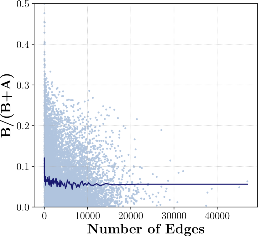
(b)

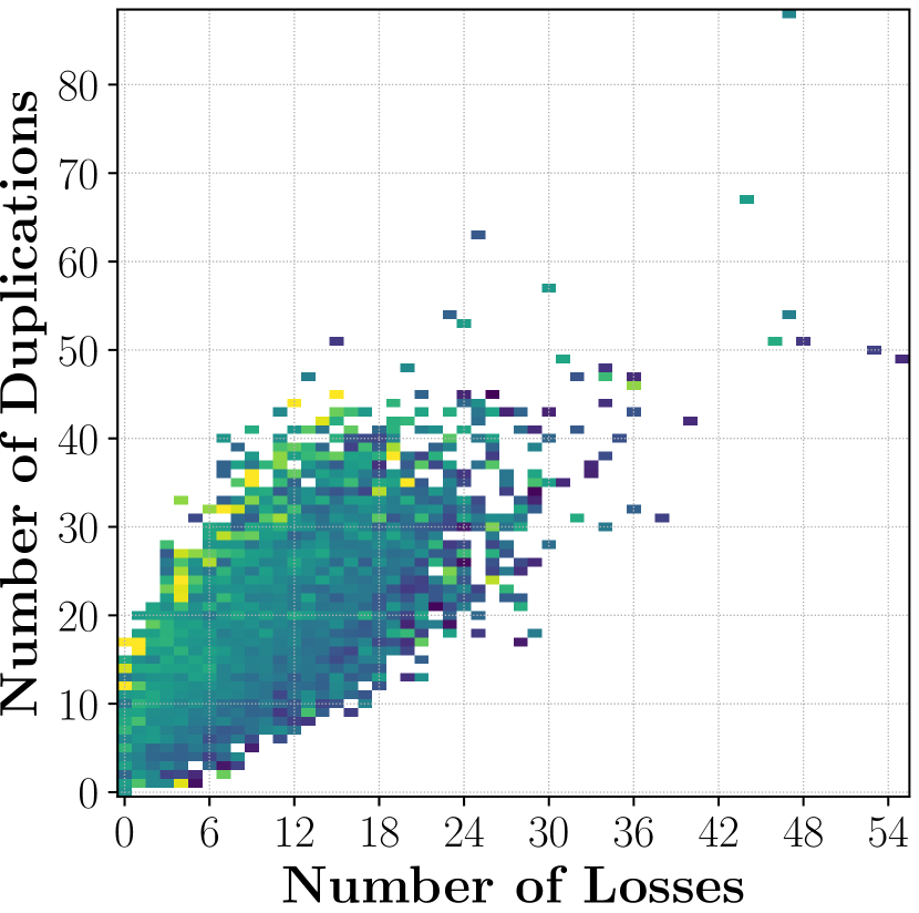
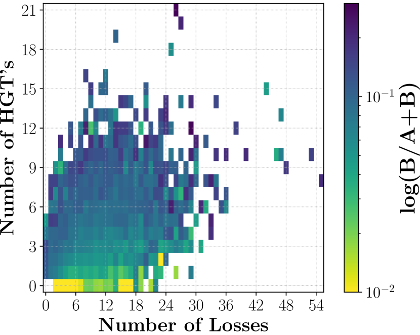
Figure 8: Relative abundance $\eta=\frac{B}{B+A}$ of (B)-RBMGs in the simulation data. Panel (a) shows the dependence on the number of edges in the BMG in every simulated scenario, and its average depicted by the line in darker blue. Scatter plots (b) show the dependence of $\eta$ on the number of duplications and losses, and HGTs and losses, respectively.

Although events that generate more than two offspring lineages are logically possible in real data, most multifurcations in phylogenetic trees are considered to be “soft polytomies”, arising from data that are insufficient to produce a fully resolved, binary trees (Purvis and Garland Jr., 1993; Kuhn et al., 2011; Sayyari and Mirarab, 2018). Type (C) 3-RBMGs thus should be very unlikely under biologically plausible assumptions on the model of evolution. Here we only consider the abundance of Type (B) components relative to all Type (A) and (B) components. We denote their ratio by $\eta$. The results are summarized in Fig. 8. We find that $\eta$ is usually below 20% and increases with the number of loss and HGT events. More precisely, 83.47% of the 14,000 scenarios have at least one Type (B) component and 16.53% do not have Type (B) components at all. Among all 3-colored connected components taken from the restrictions to any three colors, 94.41% are of Type (A) and 5.59% are of Type (B).

A graph $G$ is called $P_{4}$-sparse if every induced subgraph on five vertices contains at most one induced $P_{4}$ (Jamison and Olariu, 1992). The interest in $P_{4}$-sparse graphs derives from the fact that the cograph editing problem is solvable in linear time from $P_{4}$-sparse graphs (Liu et al., 2012). It is of immediate practical interest, therefore, to determine the abundance of $P_{4}$-sparse RBMGs that are not cographs. Among the 14,000 simulated scenarios, we found that about 20.9% of the 3-colored Type (B) components are $P_{4}$-sparse, while the majority contains “overlapping” $P_{4}$s. We then investigated the corresponding $\mathsf{S}$-thin graphs. An undirected colored graph $(G,\sigma)$ is called $\mathsf{S}$-thin if no distinct vertices are in relation $\mathsf{S}$. Two vertices $a$ and $b$ are in relation $\mathsf{S}$ if $N(a)=N(b)$ and $\sigma(a)=\sigma(b)$. Somewhat surprisingly, this yields a reversed situation, where more than two thirds of the $\mathsf{S}$-thin 3-colored Type (B) components are now $P_{4}$-sparse, while only a minority of 31.32% is not $P_{4}$-sparse. An example of an undirected colored graph $(G,\sigma)$ and its corresponding $\mathsf{S}$-thin version $(G/\mathsf{S},\sigma_{/\mathsf{S}})$, which we found during our simluations, is shown in Panel (B) of Fig. 9.

Figure 9: Top: Among our 14,000 simulated scenarios we found that a majority of 79.12% of the (not necessarily $\mathsf{S}$-thin) 3-colored Type (B) components are not $P_{4}$-sparse. For the corresponding $\mathsf{S}$-version of those 3-colored components only 31.32% are not $P_{4}$-sparse while 68.68% are $P_{4}$-sparse. Below: One of the simulated 3-colored Type (B) components $(G,\sigma)$, which is not $\mathsf{S}$-thin, and its corresponding $\mathsf{S}$-thin version $(G/\mathsf{S},\sigma_{/\mathsf{S}})$.

Next we investigated the relationship of the RBMG $G(T,\sigma)$ and the orthology graph $\Theta$ (see Fig. 10). We empirically confirmed that $E(\Theta)\subseteq E(G(T,\sigma))$ in the absence of HGT (not shown). Also following our expectations, the fraction $|E(G(T,\sigma))\setminus E(\Theta)|/|E(G(T,\sigma))|$ of false-positive orthology predictions in an RBMG is small as long as duplications and losses remain moderate (l.h.s. panel in Fig. 10). Most of the false positive orthology calls are associated with large numbers of losses for a given number of duplication.

$\frac{|E(G(T,\sigma))\setminus E(\Theta)|}{|E(G(T,\sigma))|}$

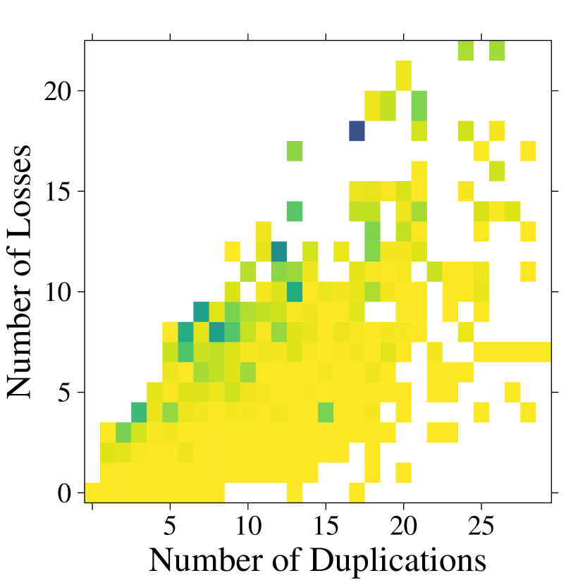
$\frac{|E(G_{4}(T,\sigma))\setminus E(\Theta)|}{|E(G_{4}(T,\sigma))|}$

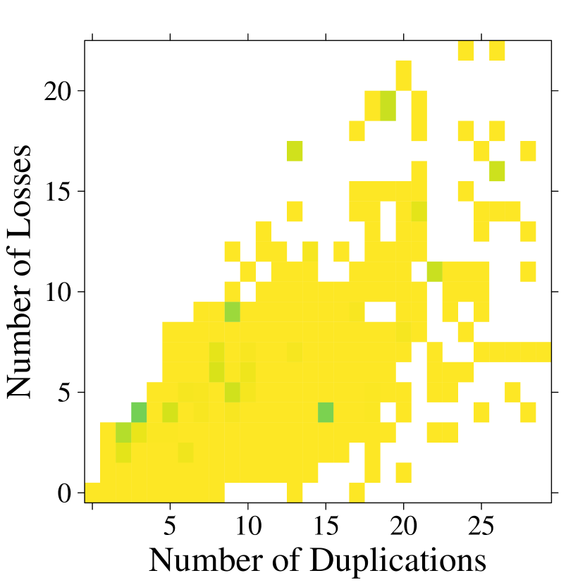
Figure 10: Fraction of non-orthology edges in the reciprocal best match graph (l.h.s.). The $x$-axis, resp., $y$-axis indicate the total number of duplications, resp., losses in the simulated scenarios. Most of the false positive orthology assignments in the l.h.s. panel are removed by deleting the middle edge of good quartets (r.h.s. panel). White background indicates no data.

We find that good quartets eliminate nearly all false positive edges from the RBMG and leave a nearly perfect orthology graph (r.h.s. panel in Fig. 10). As we have seen so far, reciprocal best matches indeed form an excellent approximation of orthology in duplication-loss scenarios. In particular, the good quartets identify nearly all false positive edges, making it easy to remove the few remaining $P_{4}$s using a generic cograph editing algorithm (Liu et al., 2012).

8 Outlook: Evolutionary Scenarios with Horizontal Gene Transfer

The benign results above beg the question how robust they are under HGT. Gene family histories with HGT have been a topic of intense study in recent years (Doyon et al., 2010; Tofigh et al., 2011; Bansal et al., 2012; Nøjgaard et al., 2018). Following the so-called DTL-scenarios as proposed e.g. by Tofigh et al. (2011); Bansal et al. (2012) we relax the notion of reconciliation maps, since ancestry is no longer preserved. We replace Axiom (R2) by

(R2w)

Weak Ancestor Preservation.
If $x\prec_{T}y$, then either $\mu(x)\preceq_{S}\mu(y)$ or $\mu(x)$ and $\mu(y)$ are incomparable w.r.t. $\prec_{S}$.

and add the following constraints

(R3.iii)

Addition to the Speciation Constraint.
If $\mu(x)\in W^{0}$, then $\mu(v)\preceq_{T}\mu(x)$ for all $v\in\mathsf{child}(x)$.

(R4)

HGT Constraint.
If $x$ has a child $y$ such that $\mu(x)$ and $\mu(y)$ are incomparable, then $x$ also has a child $y^{\prime}$ with $\mu(y^{\prime})\preceq_{S}\mu(x)$.

Property (R2w) equivalently states that if $x\prec_{T}y$, then we must not have $\mu(y)\prec_{S}\mu(x)$, which would invert the temporal order. Property (R3.iii) (which follows from (R2) but not from (R2w)) ensures that the children of speciation events are still mapped to positions that are comparable to the image of the speciation node. Condition (R4), finally, requires that every horizontal transfer event also has a vertically inherited offspring. Note that condition (R4) is void if (R2) holds. In summary the axioms (R0), (R1), (R2w), (R3.i), (R3.ii), (R3.iii), and (R4) are a proper generalization of Def. 1. We note that these axioms are not sufficient to ensure time consistency, however. We refer to Nøjgaard et al. (2018) for details. Our choice of axioms also rules out some scenarios that may appear in reality (or simulations), but which are not observable when only evolutionary divergence is available as measurement. For example, Condition (R3.ii) excludes scenarios in which HGT events have no surviving vertically inherited offspring.

We furthermore extend the event map $t$ for a gene tree $T$ to include HGT as an additional event type denoted by the symbol $\triangle$. We define $t:V(T)\to\{\circledcirc,\odot,\newmoon,\square,\triangle\}$ such that $t(u)=\triangle$ if and only if $u$ has a child $v$ such that $\mu(u)$ and $\mu(v)$ are incomparable. Since the offsprings of an HGT event are not equivalent, it is useful to introduce an edge labeling $\lambda:E(T)\to\{0,1\}$ such that $\lambda(uv)=1$ if $\mu(u)$ and $\mu(v)$ are incomparable w.r.t. $\prec_{S}$. This edge labeling is investigated in detail by Geiß et al. (2018) as the basis of Fitch’s xenology relation. Alternatively, the asymmetry can be handled by enforcing an ordering of the vertices, see (Hellmuth et al., 2017).

Evolutionary scenarios with horizontal transfer may lead to a situation where two genes $x,y$ in the same species, i.e., with $\sigma(x)=\sigma(y)$, derive from a speciation, i.e., $\operatorname{lca}_{T}(x,y)=\newmoon$. This is the case when the two lineages underwent an HGT event that transferred a copy back into the lineage in which the other gene has been vertically transmitted. We call such genes xeno-orthologs and exclude them from the orthology relation, see Fig. 11. This choice is motivated (1) by the fact that, by definition, genes of the same species cannot be recognized as reciprocal best matches, and (2) from a biological perspective they behave rather like paralogs. In scenarios with HGT we therefore modify the definition of the orthology graph such that $E(G_{1}\operatorname{\Join}G_{2})$ is replaced by

$$E(G_{1}\widetilde{\operatorname{\Join}}G_{2}):=E(G_{1})\cup E(G_{2})\cup\{uv\mid u\in V(G_{1}),v\in V(G_{2})\text{ and }\sigma(u)\neq\sigma(v)\}\,.$$ (3)

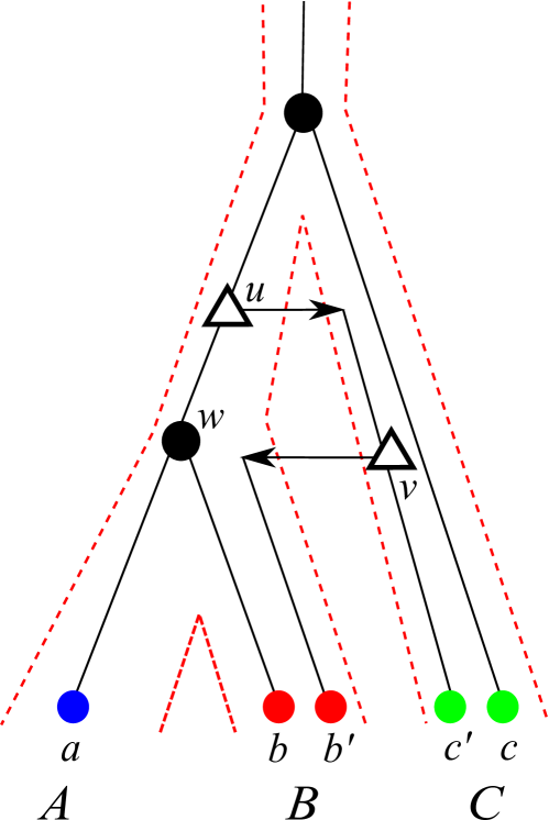
Figure 11: A gene tree $(T,t,\lambda,\sigma)$ reconciled with a species tree $S$. Here, we have two transfer edges $uv$ and $vb^{\prime}$ with $t(u)=t(v)=\triangle$. For the two children $w$ and $v$ of $u$ it holds $\sigma(L(T(w)))\cap\sigma(L(T(v)))\neq\emptyset$, a property that is shared with duplication vertices. For the two children $b^{\prime}$ and $c^{\prime}$ of $v$ it holds $\sigma(L(T(b^{\prime})))\cap\sigma(L(T(c^{\prime})))=\emptyset$, a property that is shared with speciation vertices. In this example, $c$ and $c^{\prime}$ are xeno-orthologs and the pairs $(c,c^{\prime}),(c^{\prime},c)$ will be excluded from the resulting orthology relation.

The extremal map ${\widehat{t}_{T}}$ as in Def. 4 cannot easily be extended to include HGT, as the events $\newmoon$ and $\square$ on some vertex $u$ are solely defined on two exclusive cases: either $\sigma(L(T(u_{1})))$ and $\sigma(L(T(u_{2})))$ are disjoint or not for $u_{1},u_{2}\in\mathsf{child}(u)$. Both cases, however, can also appear when we have HGT (see Fig. 11 for an example). That is, the fact that $\sigma(L(T(u_{1})))$ and $\sigma(L(T(u_{2})))$ are disjoint or not, does not help to unambiguously identify the event types in the presence of HGT.

Prop. 1 can be generalized to the case that $(T,t,\lambda,\sigma)$ contains HGT events. The existence of reconciliation maps from an event-labeled tree $(T,t,\lambda,\sigma)$ to an unknown species tree can be characterized in terms of species triples $\sigma(a)\sigma(b)|\sigma(c)$ that can be derived from $(T,t,\lambda,\sigma)$ as follows: Denote by $\mathcal{E}\coloneqq\{e\in E(T,t,\lambda,\sigma)\mid\lambda(e)=1\}$ the set of all transfer edges in the labeled gene tree and let $(T_{\mathcal{\overline{E}}},t,\sigma)$ be the forest obtained from $(T,t,\lambda,\sigma)$ by removing all transfer edges. By definition, $\mu(x)$ and $\mu(y)$ are incomparable for every transfer edge $xy$ in $T$. The set $\mathcal{S}(T,t,\lambda,\sigma)$ is the set of triples $\sigma(a)\sigma(b)|\sigma(c)$ where $\sigma(a)$, $\sigma(b)$, $\sigma(c)$ are pairwise distinct and either

1. $ab|c$ is a triple displayed by a connected component $T^{\prime}$ of $T_{\mathcal{\overline{E}}}$ such that the root of the triple is a speciation event, i.e., $t(\operatorname{lca}_{T^{\prime}}(a,b,c))=\newmoon$.

2. or $a,b\in L(T_{\mathcal{\overline{E}}}(x))$ and $c\in L(T_{\mathcal{\overline{E}}}(y))$ for some transfer edge $xy$ or $yx$ of $T$.

Proposition 5.

(Hellmuth, 2017) Given an event-labeled, leaf-labeled tree $(T,t,\sigma)$. Then, there is a reconciliation map $\mu:V(T)\to V(S)\cup E(S)$ to some species tree $S$ if and only if $\mathcal{S}(T,t,\sigma)$ is compatible. In this case, $(T,t,\sigma)$ can be reconciled with every species tree $S$ that displays the triples in $\mathcal{S}(T,t,\sigma)$.

Here, we have not added additional constraints on reconciliation maps that ensure that the map is also “time-consistent”, that is, genes do not travel “back” in the species tree, see (Nøjgaard et al., 2018) for further discussion on this. However, Prop. 5 gives at least a necessary condition for the existence of time-consistent reconciliation maps. A simple proof of Prop. 5 for the case that $T$ is binary and does not contain HGT events can be found in (Hernandez-Rosales et al., 2012). Moreover, generalizations of reconciling event-labeled gene trees with species networks have been established by Hellmuth et al. (2019).

(a)	(b)	(c)
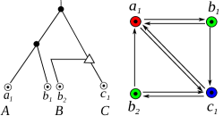
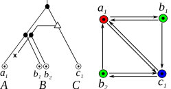
(d)	(e)	(f)

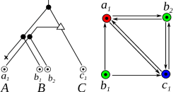
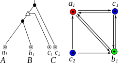
Figure 12: Scenarios with four genes, three species, and a single HGT event for which RBMG $G(T,\sigma)$ and orthology relation $\Theta(T,t)$ differ. The BMG is shown for each scenario. In the first two cases (a) and (b), $G(T,\sigma)$ contains an induced $P_{4}$ in the RBMG, which might serve as indication for HGT events. In the remaining cases, the $G(T,\sigma)$ is a cograph, which does not represent the correct orthology relation, however. In scenario (c), the graph $G(T,\sigma)$ is a triangle with an attached edge, while the orthology relation is given by $\Theta(T,t)=K_{4}-e-f$ with the missing edges $e=a_{1}a_{2}$ and $f=a_{1}b_{1}$, where the latter results from the xenologous pair $a_{2},b_{1}$. In the remaining three cases (d)-(f), the RBMG is $K_{3}\mathbin{\mathchoice{\leavevmode\vtop{\halign{\hfil$\m@th\displaystyle#$\hfil\cr\cup\cr\cdot\crcr}}}{\leavevmode\vtop{\halign{\hfil$\m@th\textstyle#$\hfil\cr\cup\cr\cdot\crcr}}}{\leavevmode\vtop{\halign{\hfil$\m@th\scriptstyle#$\hfil\cr\cup\cr\cdot\crcr}}}{\leavevmode\vtop{\halign{\hfil$\m@th\scriptscriptstyle#$\hfil\cr\cup\cr\cdot\crcr}}}}K_{1}$ compared to the orthology relation $\Theta(T,t)=K_{4}-e$, where the edge $e$ again corresponds to the edge between genes of the same species.

In contrast to pure DL scenarios, it is no longer guaranteed that all true orthology relationships are also reciprocal best matches. Fig. 12 gives counterexamples. In three of these scenarios the RBMG contains an induced $P_{4}$ that mimics a good quartet. Removal of the middle edge of good quartets therefore not only reduces false positives in DL scenarios but also introduces additional false negatives in the presence of HGT.

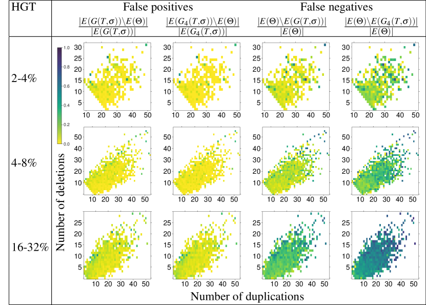
Figure 13: Dependence of the fraction of false positive and false negative orthology assignments in RBMGs in the presence of different levels of HGT, measured as percentage of HGT events among all events in the simulated true gene trees $\widetilde{T}$. As in Fig. 10, data are shown as functions of the number of duplication and loss events in the scenario. While the number of false positives seems to depend very little on even high levels of HGT, the fraction of false negatives is rapidly increasing. Since HGT introduces good quartets that comprise only true orthology edges, their removal further increases the false positive rate (last column).

9 Discussion

In the theoretical part of this contribution we have clarified the relationships between (reciprocal) best match graphs (RBMGs), orthology, reconciliation map, gene tree, species tree, and event map for the case of duplication loss scenarios.

The orthology graph $\Theta$ is necessarily a subgraph of the RBMG. In the absence of HGT, RBMGs therefore produce only false positive but no false negative orthology assignments. Using not only reciprocal best matches but all best matches, furthermore, shows that good quartets identify almost all false positive edges. Removing the central edge of all good quartets in $(\mathaccent 382{G},\sigma)$ yields nearly perfect orthology estimates. This, however, implies that orthology inference is not solely based on reciprocal best matches. Instead, it is necessary to also include certain directional best matches, namely those that identify good quartets.

We observed that a small number of HGT events can cause large deviations between the RBMG $(G,\sigma)$ and the orthology graph $\Theta$. However, we have considered here the worst-case scenario, where HGT events occur between relatively closely related organisms. While this is of utmost relevance in some cases, for instance for toxin and virulence genes in bacteria, it is of little concern e.g. for the evolution of animals. In the latter case, xenologs almost always originate from bacteria or viruses, i.e., from outgroups. The xenologs then form their own group of co-orthologs and behave as if they would have been lost in the species outside the subtree that received the horizontally transfered gene.

From a more theoretical point of view, our empirical findings in the HGT case beg two questions: (1) Are there local features in the (R)BMG that make it possible to unambiguously identify HGT, at least in some cases? (2) What kind of additional information can be integrated to distinguish good quartets arising from duplication/loss events that can be safely removed from those that are introduced by HGT and should be “repaired” in a different manner. Most obviously, one may ask whether the Fitch relation is sufficient (we conjecture that this is the case) (Geiß et al., 2018; Hellmuth and Seemann, 2019), or whether it suffices to know that a leaf is a (recent) result of transfer (we conjecture that this is not enough in general).

The identification of edges in the RBMG that should or should not be removed has important implication for orthology detection approaches that enforce the cograph structure of the predicted orthology relation by means of cograph editing. While this is an NP-complete problem (Liu et al., 2012) in general, the complexity of the colored version, i.e., editing a properly colored graph to the nearest hc-cograph remains open. The removal of false positive edges identified by good quartets empirically reduces the number of induced $P_{4}$s drastically. This observation also suggests to consider hc-cograph editing with a given best match relation. We suspect that the additional knowledge of the directed edges makes the problem tractable since it already implies a unique least resolved tree that captures much of the cograph structure.

Cograph editing would be fully content with hc-cographs, i.e., co-RBMGs. These are not necessarily “biologically feasible” in the sense that they can be reconciled with a species tree. It will therefore be of interest to consider the problem of editing an hc-cograph to another hc-cograph that is reconcilable with some or a given species tree – a problem that has been considered already for orthology relations (Lafond et al., 2016; Lafond and El-Mabrouk, 2014). Since the obstructions are conflicting triples with a speciation at their top node, the offending data are conflicting orthology assignments. It seems natural therefore to phrase the problem not as an arbitrary editing problem but instead to ask for a maximal induced sub-hc-cograph that implies a compatible triple set. If it is indeed true that triples necessarily displayed by the species tree can be extracted directly from the c(R)BMG, it will be of practical use to consider the corresponding edge deletion problem for c(R)BMGs. In particular, it would be interesting to know whether the latter problem is the same as asking for the maximal compatible subset of triples implied by the c(R)BMG or co-BMG?

Appendix A Extraction of Graphs from Simulated Evolutionary Scenarios

The simulations of evolutionary scenarios (described in the main text) result in an event-labeled gene tree $(T,t,\sigma)$ as well as an explicit reconciliation map $\mu:V(T)\to V(S)\cup E(S)$. From these data we have to construct the orthology graph $\Theta(T,t)$ and the RBMG $G(T,\sigma)$. This can be achieved in $O(L^{2})$ time using Tarjan’s off-line lowest common ancestors algorithm (Tarjan, 1979; Gabow and Tarjan, 1983) to first tabulate $\operatorname{lca}_{T}(x,y)$ for all $x,y\in L$ in quadratic total time or with the help of additional data structures that then allow to answer least common ancestor queries in constant time (Harel and Tarjan, 1984; Schieber and Vishkin, 1988). As show below, it is also possible to avoid computation of the $\operatorname{lca}()$ function altogether.

A.1 Orthology Graphs

The orthology relation $\Theta(T,t)$ is easily constructed from the event-labeled gene tree $(T,t)$ by a simple recursive construction. For each $v\in\widetilde{T}$ we define a graph $\Theta(v)$ recursively: if $v$ is a leaf, then $\Theta(v)$ is the $K_{1}$ with vertex set $\{v\}$ whenever $v$ is an extant gene and $\Theta(v)=\emptyset$, the empty graph, if $v$ is a loss event. For inner vertices we set

$$\Theta(v)=\begin{cases}\displaystyle\mathop{\vphantom{\sum}\mathchoice{\vbox{\hbox{\leavevmode\resizebox{9.00005pt}{}{$\Join$}}}}{\vbox{\hbox{\leavevmode\resizebox{10.00012pt}{}{$\Join$}}}}{\vbox{\hbox{\leavevmode\resizebox{7.00009pt}{}{$\Join$}}}}{\vbox{\hbox{\leavevmode\resizebox{5.00006pt}{}{$\Join$}}}}}\slimits@_{u\in\mathsf{child}(v)}\Theta(u)&\textrm{if }t(v)=\newmoon\\ \displaystyle\bigcup_{u\in\mathsf{child}(v)}\Theta(u)&\textrm{otherwise}\end{cases}$$ (4)

Since $H\operatorname{\Join}\emptyset=H\cup\emptyset=H$, there is no contribution of the loss-leafs. Thus $\Theta(v)$ can be computed in exactly the same manner from the observable gene tree $T$. Hence, $\Theta(\rho_{T})=\Theta(\rho_{\widetilde{T}})=:\Theta$ is the orthology graph of the scenario. Note that the planted root $0_{T}$ does not appear as the last common ancestor of any two leaves in $L(T)$, hence it suffices to consider the root. Although the next result is an immediate consequence of the definition of cographs and their corresponding cotrees (Corneil et al., 1981):

Lemma 1.

Let $(T,t,\sigma)$ be an event-labeled, leaf-labeled tree. Then $xy\in E(\Theta(v))$ if and only if $t(\operatorname{lca}_{T}(x,y))=\newmoon$.

By construction, $\Theta(u)$ is an induced subgraph of $\Theta(v)$ whenever $u\preceq_{T}v$. It is thus sufficient to store the binary $|L|\times|L|$ adjacency matrix of $\Theta$. Traversing $T$ in post-order, one sets $\Theta_{xy}=1$, i.e., $xy\in E(\Theta)$, for all $xy$ with $x\in L(T(u_{1}))$ and $y\in L(T(u_{2}))$ where $u_{1}$ and $u_{2}$ are distinct children of $v$, if and only if $v$ is a speciation vertex. Since the pair $x,y$ is considered exactly once, namely when $v=\operatorname{lca}(x,y)$ is encountered in the traversal of $T$, the total effort is $O(|L|^{2})$.

A.2 Best Match Graphs

In order to compute the BMG $\mathaccent 382{G}(T,\sigma)$ we associate every inner vertex $v$ with the lists $L_{r}(v):=\{x\in L(T(v))|\sigma(x)=r\}$ of leaves below $v$ with color $r$. We have $L_{r}(v)=\bigcup_{u\in\mathsf{child}(v)}L_{r}(u)$ for inner vertices, while leaves are initialized with $L_{r}(v)=\{v\}$ if $\sigma(v)=r$, and $L_{r}(v)=\emptyset$ if $\sigma(v)\neq r$. Again this can be achieved in not more than quadratic time. Now define $C_{\neg s}(v):=\{u\in\mathsf{child}(v)|L_{s}(u)=\emptyset\}$ and $C_{s}(v):=\{u\in\mathsf{child}(v)|L_{s}(u)\neq\emptyset\}$. Best matches can be retrieved directly from these auxiliary sets:

Lemma 2.

Let $u_{1}$ and $u_{2}$ be two distinct children of some inner vertex $v$ of the leaf-colored tree $(T,\sigma)$ and let $x\in L(T(u_{1}))$ with $\sigma(x)=r$ and $y\in L(T(u_{2}))$ with $\sigma(y)=s\neq r$. Then $(x,y)$ is a best match in $(T,\sigma)$ if and only if

$$u_{1}\in C_{r}(v)\cap C_{\neg s}(v)\quad\textrm{and}\quad u_{2}\in C_{s}(v).$$

Proof.

If $L_{s}(u_{1})=\emptyset$, then there is no best match of color $s$ for $x$ in $L(T(u_{1}))$, i.e., any best match $\sigma(y^{\prime})=s$ satisfies $v\preceq\operatorname{lca}(x,y^{\prime})$. From $\operatorname{lca}(x,y)=v$ we see that $(x,y)$ is indeed a best match. On the other hand, if $L_{s}(u_{1})\neq\emptyset$, then there is a leaf $y^{\prime}\in L_{s}(u_{1})$ with $\operatorname{lca}(x,y^{\prime})\preceq u_{1}\prec v=\operatorname{lca}(x,y)$, and thus $y$ is not a best match for $x$. ∎∎

Algorithm 1 Construction of $\mathaccent 382{G}(T,\sigma)$

0  leaf-colored tree $(T,\sigma)$

  for all leaves $v$ of $T$, colors $r$ do

     $L(T(v))=\{v\}$

     if $\sigma(v)=r$ then

        $\ell_{vr}=1$

     else

        $\ell_{vr}=0$

  for all inner vertices $v$ of $T$ in postorder do

     for all $u_{1},u_{2}\in\mathsf{child}(v)$, $u_{1}\neq u_{2}$ do

        for all $x\in L(T(u_{1}))$ and $y\in L(T(u_{2}))$ do

           $(x,y)\in\mathaccent 382{G}(T,\sigma)$ if $\ell_{u_{1}\sigma(y)}=0$

     $L(T(v))=\bigcup_{u\in\mathsf{child}(v)}L(T(u))$

     for all $u\in\mathsf{child}(v)$, colors $r\in S$ do

        $\ell_{vr}=1$ if $\ell_{ur}=1$

This observation yields the very simple way to construct $\mathaccent 382{G}(T,\sigma)$. Algorithm 1 iterates over all pairs of vertices $x,y\in L$ such that each pair is visited exactly once by considering for every interior vertex $v$ exactly the pairs that are members of two distinct subtrees rooted at children $u_{1}$ and $u_{2}$ of $v$. Since $y\in L_{\sigma(y)}(u_{2})$ and $x\in L_{\sigma(x)}(u_{1})$ is guaranteed by construction, $(x,y)$ is a best match if and only if $L_{\sigma(y)}(u_{1})=\emptyset$ by Lemma 2. Using the precomputed binary variable $\ell_{vr}$ with value $1$ if $L_{r}(v)\neq\emptyset$ and $\ell_{vr}=0$ otherwise, this can be done in constant time $O(|L|)$. By traversing $T$ in postorder, finally, we can compute the lists of leaves $L(v)$ on the fly. Since no subtree is revisited, there is no need to retain the $L(T(u))$ for the children, i.e., for each vertex $v$, the lists of its children can simply be concatenated. Similarly, the variables $\ell_{vr}$ can be obtained while traversing $T$ using the fact that $\ell_{vr}=1$ if and only if $\ell_{ur}=1$ for at least one of its children. Hence, Algorithm 1 runs in $O(|L|^{2})$ time with $O(|L|\,|S|)$ memory using a single postorder traversal of $T$.

The RBMG $G(T,\sigma)$ is now easily obtained from the BMG $\mathaccent 382{G}(T,\sigma)$ by extracting its symmetric part. Clearly the effort for this step is also bounded by $O(|L|^{2})$.

A.3 Good Quartets

We have seen in Section 6 that at least some false positive edges are identified by good quartets. A convenient way of listing all good quartets $Q$ in $(\mathaccent 382{G},\sigma)$ makes use of the degree sequence of $\mathaccent 382{G}$, that is, the list $\alpha=((\alpha_{x}^{+},\alpha_{x}^{-})|x\in V(\mathaccent 382{G}))$ of pairs $(\alpha_{x}^{+},\alpha_{x}^{-})$ where $\alpha_{x}^{+}$ is the out-degree and $\alpha_{x}^{-}$ is the in-degree of the vertex $x\in V(\mathaccent 382{G})$ and the list is ordered in positive lexicographical order. One easily checks that a good quartet contains neither a 2-switch nor an induced 3-cycle, hence $Q$ is uniquely defined by its degree sequence $((2,1),(2,3),(2,3),(2,1))$ as a consequence of (Cloteaux et al., 2014, Thm. 1). Regarding the coloring, it suffices to check that the two endpoints, that is, the vertices with indegree $1$, have the same color $\sigma(u)=\sigma(x)$. This already implies $\sigma(v),\sigma(w)\neq\sigma(u)=\sigma(x)$. Since there is an edge between $v$ and $w$, we also have $\sigma(v)\neq\sigma(w)$, i.e., the colors are determined up to a permutation of colors. The false positive edge is the one connecting the two vertices with outdegree $3$.

Appendix B Additional Information on Simulated Scenarios

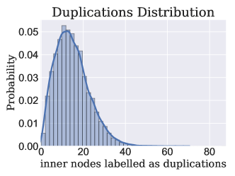
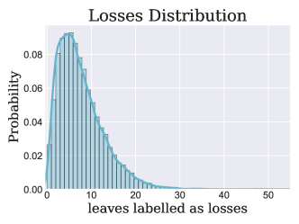
(a) (b) (c) (d)

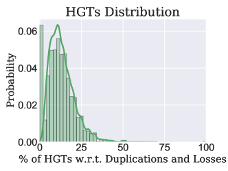
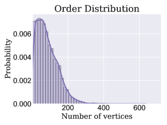
Max. Min. Average Species 100 3 44.5 Extant genes 722 3 84.62 Speciations ($S_{n}$) 667 2 73.46 Duplications ($D_{n}$) 88 0 14.66 Losses ($L_{n}$) 55 0 7.41 HGT ($H_{n}\%$) 100% 0% 11.76%

Figure 14: Summary statistics of the 14,000 simulated scenarios. (a)–(c) Distributions of fraction of duplications, losses, and HGTs, respectively in the true gene trees $\widetilde{T}$. (d) Distribution of the number of extant genes in the observable gene tree $T$ and thus the number of vertices (order) of the best match graph $G(T,\sigma)$. The spline in each panel is a kernel density estimate.

Table 1: We simulated 11 batches with different ranges for the rates of duplications, losses, and HGT (columns 3 to 5), where the rates have been varied in steps of 0.01. In each batch, we simulated for each combination of rates exactly one scenario. The second column shows the total number of scenarios for each batch.

Batch	# Scenarios	Duplication rates	Loss rates	HGT rates	# Species
1	1000	0.75 - 0.84	0.7 - 0.79	0.1 - 0.19	3-100
2	1000	0.85 - 0.94	0.85 - 0.94	0.1 - 0.19	3-100
3	1000	0.80 - 0.89	0.80 - 0.89	0.1 - 0.19	3-100
4	1000	0.70 - 0.79	0.70 - 0.79	0.1 - 0.19	3-100
5	1000	0.90 - 0.99	0.90 - 0.99	0.1 - 0.19	3-100
6	1000	0.85 - 0.94	0.75 - 0.84	0.1 - 0.19	3-100
7	1000	0.90 - 0.99	0.90 - 0.99	0.15 - 0.24	3-100
8	1000	0.90 - 0.99	0.90 - 0.99	0.15 - 0.24	3-100
9	1000	0.65 - 0.74	0.65 - 0.74	0.10 - 0.19	3-100
10	1000	0.85 - 0.94	0.75 - 0.84	0.15 -0.24	3-100
11	4000	0.75 - 0.94	0.75 - 0.94	0.15 -0.24	3-50

Appendix C False Positive Edges in Non-Cograph 3-RBMGs

In the following, we identify further false positive orthology assignments in the RBMG based on results that we recently derived in Geiß et al. (2019b). We start by defining a color-preserving thinness relation that has been introduced in Geiß et al. (2019b):

Definition 1.

For an undirected colored graph $(G,\sigma)$ two vertices $a$ and $b$ are in relation $\mathsf{S}$, in symbols $a\mathsf{S}b$, if $N(a)=N(b)$ and $\sigma(a)=\sigma(b)$. The equivalence class of $a$ is denoted by $[a]$. $(G,\sigma)$ is called $\mathsf{S}$-thin if no two distinct vertices are in relation $\mathsf{S}$.

C.1 Type (B) 3-RBMGs

Let $(G,\sigma)$ be a connected $\mathsf{S}$-thin 3-RBMG of Type (B). Lemma 25 of (Geiß et al., 2019b) then implies that $(G,\sigma)$ contains an induced path $P:=\langle\widehat{x}_{1}\widehat{y}\widehat{z}\widehat{x}_{2}\rangle$ with three distinct colors $\sigma(\widehat{x}_{1})=\sigma(\widehat{x}_{2})=:r$, $\sigma(\widehat{y})=:s$, and $\sigma(\widehat{z})=:t$, and $N_{r}(\widehat{y})\cap N_{r}(\widehat{z})=\emptyset$ such that the vertex sets

• $L_{t,s}^{P}\coloneqq\{y\mid\langle xy\widehat{z}\rangle\in\mathscr{P}_{3}\text{ for any }x\in N_{r}(y)\}$,

• $L_{t,r}^{P}\coloneqq\{x\mid N_{r}(y)=\{x\}\text{ and }\langle xy\widehat{z}\rangle\in\mathscr{P}_{3}\}\cup\{x\mid x\in L[r],\,N_{s}(x)=\emptyset,\,L[s]\setminus L_{t,s}^{P}\neq\emptyset\}$,

• $L_{s,t}^{P}\coloneqq\{z\mid\langle xz\widehat{y}\rangle\in\mathscr{P}_{3}\text{ for any }x\in N_{r}(z)\}$,

• $L_{s,r}^{P}\coloneqq\{x\mid N_{r}(z)=\{x\}\text{ and }xz\widehat{y}\in\mathscr{P}_{3}\}\cup\{x\mid x\in L[r],N_{t}(x)=\emptyset,L[t]\setminus L_{s,t}^{P}\neq\emptyset\}$,

• $L_{t}^{P}\coloneqq L_{t,s}^{P}\cup L_{t,r}^{P}$,

• $L_{s}^{P}\coloneqq L_{s,t}^{P}\cup L_{s,r}^{P}$, and

• $L_{*}^{P}\coloneqq L\setminus(L_{t}^{P}\cup L_{s}^{P})$

satisfy the following conditions:

(B2.a)

If $x\in L_{*}^{P}[r]$, then $N(x)=L_{*}^{P}\setminus\{x\}$,

(B2.b)

If $x\in L_{t}^{P}[r]$, then $N_{s}(x)\subset L_{t}^{P}$ and $|N_{s}(x)|\leq 1$, and $N_{t}(x)=L_{*}^{P}[t]$,

(B2.c)

If $x\in L_{s}^{P}[r]$, then $N_{t}(x)\subset L_{s}^{P}$ and $|N_{t}(x)|\leq 1$, and $N_{s}(x)=L_{*}^{P}[s]$

(B3.a)

If $y\in L_{*}^{P}[s]$, then $N(y)=L_{s}^{P}\cup(L_{*}^{P}\setminus\{y\})$,

(B3.b)

If $y\in L_{t}^{P}[s]$, then $N_{r}(y)\subset L_{t}^{P}$ and $|N_{r}(y)|\leq 1$, and $N_{t}(y)=L[t]$,

(B4.a)

If $z\in L_{*}^{P}[t]$, then $N(z)=L_{t}^{P}\cup(L_{*}^{P}\setminus\{z\})$,

(B4.b)

If $z\in L_{s}^{P}[t]$, then $N_{r}(z)\subset L_{s}^{P}$ and $|N_{r}(z)|\leq 1$, and $N_{s}(z)=L[s]$.

By construction, $\sigma(L_{t}^{P})=\{r,s\}$ and $\sigma(L_{s}^{P})=\{r,t\}$ and, as a consequence of Lemma 25 of Geiß et al. (2019b), the sets $L_{s}^{P}$, $L_{t}^{P}$, and $L_{*}^{P}$ form a partition of $V(G)$. Furthermore, Lemma 33 of Geiß et al. (2019b) implies that any 3-colored induced path $P$ of the form $(r,s,t,r)$ that satisfies (B2.a) to (B4.b) is a good quartet w.r.t. some $(T,\sigma)$ explaining a BMG $(\mathaccent 382{G},\sigma)$ that contains $(G,\sigma)$ as its symmetric part.

Our goal is to identify edges in $(G,\sigma)$ that can cannot be present in the orthology graph $\Theta$. To this end we extend the leaf sets $L^{P}_{*},L^{P}_{s},L^{P}_{t}$ that have been introduced in Geiß et al. (2019b) for $\mathsf{S}$-thin 3-RBMGs, to general 3-RBMGs:

Definition 2.

Let $(G,\sigma)$ be a 3-RBMG of Type (B) with vertex set $L$ and colors $S=\{r,s,t\}$, and $(G/\mathsf{S},\sigma_{/\mathsf{S}})$ with vertex set $\overline{L}$ be its $\mathsf{S}$-thin version. We set

$$L_{s}^{P} \coloneqq\{x\mid x\in L,[x]\in\overline{L}_{s}^{P}\}$$

$$L_{t}^{P} \coloneqq\{x\mid x\in L,[x]\in\overline{L}_{t}^{P}\}$$

$$L_{*}^{P} \coloneqq\{x\mid x\in L,[x]\in\overline{L}_{*}^{P}\}$$

if $(G,\sigma)$ is of Type (B) and $(G/\mathsf{S},\sigma_{/\mathsf{S}})$ B-like w.r.t. to the induced path $P$.

The cases of Type (B) and (C) 3-RBMGs will be treated separately, starting with Type (B). We first need a technical result:

Lemma 1.

Let $(G,\sigma)$ be a connected 3-RBMG of Type (B) with vertex set $L$, $(G/\mathsf{S},\sigma_{/\mathsf{S}})$ its $\mathsf{S}$-thin version with vertex set $\overline{L}$, and $(T,\sigma)$ a leaf-labeled tree that explains $(G,\sigma)$. Moreover, let $P\coloneqq\langle[\widetilde{x}_{1}][\widetilde{y}][\widetilde{z}][\widetilde{x}_{2}]\rangle$ for some good quartet $\langle\widetilde{x}_{1}\widetilde{y}\widetilde{z}\widetilde{x}_{2}\rangle$ in $\mathaccent 382{G}(T,\sigma)$, and set $v\coloneqq\operatorname{lca}_{T}(\widetilde{x}_{1},\widetilde{x}_{2},\widetilde{y},\widetilde{z})$. Then the leaf sets $L_{s}^{P}$, $L_{t}^{P}$, and $L_{*}^{P}$, where $\sigma(\widetilde{x}_{1})=\sigma(\widetilde{x}_{2})=r$, $\sigma(\widetilde{y})=s$, and $\sigma(\widetilde{z})=t$, satisfy:

• $L_{t}^{P},L_{s}^{P}\subseteq L(T(v))$,

• If $L_{c}^{P}\cap L(T(v^{\prime}))\neq\emptyset$ for some $v^{\prime}\in\mathsf{child}(v)$ and $c\in\{s,t\}$, then

  • $L_{\overline{c}}^{P}\cap L(T(v^{\prime}))=\emptyset$, where $\overline{c}\in\{s,t\},\overline{c}\neq c$,

  • $\sigma(L(T(v^{\prime})))\subseteq\sigma(L_{c}^{P})$,

• $\operatorname{lca}_{T}(a,b)=v$ for any $a\in L_{*}^{P}$, $b\notin L_{*}^{P}$ with $ab\in E(G)$.

Proof.

Throughout this proof we will often use the fact that $xy\in E(G)$ if and only if $[x][y]\in E(G/\mathsf{S})$ for any $x,y\in L$ (cf. Lemma 5 of Geiß et al. (2019b)).

Lemma 25 of Geiß et al. (2019b) implies $[\widetilde{x}_{1}],[\widetilde{y}]\in\overline{L}_{t}^{P}$ and $[\widetilde{x}_{2}],[\widetilde{z}]\in\overline{L}_{s}^{P}$, thus, by definition, we have $\widetilde{x}_{1},\widetilde{y}\in L_{t}^{P}$ and $\widetilde{x}_{2},\widetilde{z}\in L_{s}^{P}$. Moreover, by Lemma 36 of Geiß et al. (2019b), there exist distinct children $v_{1},v_{2}\in\mathsf{child}(v)$ such that $\widetilde{x}_{1},\widetilde{y}\preceq_{T}v_{1}$ and $\widetilde{x}_{2},\widetilde{z}\preceq_{T}v_{2}$. Therefore $\widetilde{y}\widetilde{z}\in E(G)$ implies $\sigma(L(T(v_{1})))=\{r,s\}$; otherwise there exists a leaf $z^{\prime}\in L(T(v_{1}))\cap L[t]$ which implies $\operatorname{lca}_{T}(\widetilde{y},z^{\prime})\prec_{T}v=\operatorname{lca}_{T}(\widetilde{y},\widetilde{z})$; a contradiction to $\widetilde{y}\widetilde{z}\in E(G)$. Analogously we obtain $\sigma(L(T(v_{2})))=\{r,t\}$.

(i) By symmetry, it suffices to consider $L_{t}^{P}$ in more detail, analogous arguments can then be applied to $L_{s}^{P}$. Let $a\in L_{t}^{P}$, or equivalently $[a]\in\overline{L}_{t}^{P}$ by definition, and suppose first $\sigma(a)=s$. Then Property (B3.b) implies $[a][\widetilde{z}]\in E(G/\mathsf{S})$. As a consequence of Lemma 5 of Geiß et al. (2019b) we thus have $a\widetilde{z}\in E(G)$. Hence, $\widetilde{y}\widetilde{z}\in E(G)$ implies $\operatorname{lca}_{T}(a,\widetilde{z})=\operatorname{lca}_{T}(\widetilde{y},\widetilde{z})=v$ and thus, $a\preceq_{T}v$. We therefore conclude $L_{t}^{P}\cap L[s]\subseteq L(T(v))$. Now assume $\sigma(a)=r$. By Property (B2.b), we either have $N_{s}([a])=\emptyset$ or there exists a vertex $y\in L[s]$ such that $[y]\in\overline{L}_{t}^{P}$ and $N_{s}([a])=\{[y]\}$. In the latter case, since $[y]\in\overline{L}_{t}^{P}$ implies $y\in L_{t}^{P}$ and, in addition, it holds $L_{t}^{P}\cap L[s]\subseteq L(T(v))$, we have $y\preceq_{T}v$. Moreover, by (B3.b), it holds $[\widetilde{x}_{2}][y]\notin E(G/\mathsf{S})$, hence $\widetilde{x}_{2}y\notin E(G)$. As a consequence of the latter and the fact that $[a][y]\in E(G/\mathsf{S})$ implies $ay\in E(G)$, it must hold $\operatorname{lca}_{T}(a,y)\prec_{T}\operatorname{lca}_{T}(\widetilde{x}_{2},y)\preceq_{T}v$ and thus, $a\preceq_{T}v$. Otherwise, if $N_{s}([a])=\emptyset$, then there must exist a leaf $z\in L[t]$ such that $[z]\in N_{t}([a])$ due to the connectedness of $G/\mathsf{S}$, which is implied by the connectedness of $G$ (cf. Lemma 5 of Geiß et al. (2019b)). Since $[a]\in\overline{L}_{t}^{P}$, Properties (B4.a) and (B4.b) immediately imply $[z]\in\overline{L}_{*}^{P}$. Then, by (B4.a), the edge $[\widetilde{x}_{1}][z]$ must be contained in $G/\mathsf{S}$, thus $\widetilde{x}_{1}z\in E(G)$. Since $\widetilde{x}_{1},\widetilde{z}\preceq_{T}v$ by Lemma 36 of Geiß et al. (2019b), it must thus hold $\operatorname{lca}_{T}(\widetilde{x}_{1},z)\preceq_{T}\operatorname{lca}_{T}(\widetilde{x}_{1},\widetilde{z})\preceq_{T}v$. Therefore $\widetilde{x}_{1}z,az\in E(G)$ implies $\operatorname{lca}_{T}(a,z)=\operatorname{lca}_{T}(\widetilde{x}_{1},z)\preceq_{T}v$ and thus, $a\preceq_{T}v$. Hence, $L_{t}^{P}\cap L[r]\subseteq L(T(v))$, which finally implies $L_{t}^{P}\subseteq L(T(v))$.

(ii) By symmetry, it again suffices to consider the case $c=t$. Let $a\in L_{t}^{P}\cap L(T(v^{\prime}))$ for some $v^{\prime}\in\mathsf{child}(v)$. Note that, by (i), such a leaf $a$ and inner vertex $v^{\prime}$ must exist. We need to distinguish the two Cases (1) $\sigma(a)=s$ and (2) $\sigma(a)=r$.

Consider first Case (1), thus in particular $s\in\sigma(L(T(v^{\prime})))$. Then, as $\sigma(L(T(v_{2})))=\{r,t\}$, we have $v^{\prime}\neq v_{2}$ and thus, $\operatorname{lca}_{T}(a,\widetilde{z})=v$. Hence, as $[a][\widetilde{z}]\in E(G/\mathsf{S})$ by Property (B3.b) and therefore, $a\widetilde{z}\in E(G)$, we can conclude $t\notin\sigma(L(T(v^{\prime})))$ by analogous arguments as just used for showing $\sigma(L(T(v_{1})))=\{r,s\}$. This implies (ii.b). Now assume, for contradiction, that there exists a leaf $x\in L(T(v^{\prime}))\cap L_{s}^{P}$. Since $t\notin\sigma(L(T(v^{\prime})))$ and, by definition, $s\notin\sigma(L_{s}^{P})$, this leaf $x$ must be of color $r$. Clearly, either there exists a leaf $y\in L[s]$ such that $xy\in E(G)$ or $N_{s}(x)=\emptyset$. In the first case, we have $[x][y]\in E(G/\mathsf{S})$ and thus, by (B2.c), $[y]\in\overline{L}_{*}^{P}$ which implies $y\in L_{*}^{P}$. In particular, as $s\in\sigma(L(T(v^{\prime})))$ and $xy\in E(G)$ implies $\operatorname{lca}_{T}(x,y)\preceq_{T}\operatorname{lca}_{T}(x,y^{\prime})$ for any $y^{\prime}\in L[s]$, we can conclude $y\preceq_{T}v^{\prime}$. Moreover, since $[\widetilde{x}_{2}]\in\overline{L}_{s}^{P}$, Property (B3.a) implies $[\widetilde{x}_{2}][y]\in E(G/\mathsf{S})$ and thus, $\widetilde{x}_{2}y\in E(G)$. However, since $v^{\prime}\neq v_{2}$, we have $\operatorname{lca}_{T}(x,y)\preceq_{T}v^{\prime}\prec_{T}v=\operatorname{lca}_{T}(\widetilde{x}_{2},y)$; a contradiction to $\widetilde{x}_{2}y\in E(G)$. We thus conclude $N_{s}(x)=\emptyset$. Hence, as $G$ is connected, there must exist a leaf $z^{\prime}$ of color $t$ such that $xz^{\prime}\in E(G)$, which implies $[x][z^{\prime}]\in E(G/\mathsf{S})$. By Property (B2.c), we have $[z^{\prime}]\in\overline{L}_{s}^{P}$ and therefore, (B4.b) implies $N_{r}([z^{\prime}])=\{[x]\}$. Since $t\notin\sigma(L(T(v^{\prime})))$, there is a $v^{\prime\prime}\in\mathsf{child}(v)\setminus\{v^{\prime}\}$ such that $z^{\prime}\preceq_{T}v^{\prime\prime}\prec_{T}v$. From $xz^{\prime}\in E(G)$ and $\operatorname{lca}_{T}(x,z^{\prime})=v$, we conclude that $r\notin\sigma(L(T(v^{\prime\prime})))$. Moreover, Lemma 10 of Geiß et al. (2019b) implies that there exist leaves $x^{\prime},y^{\prime}\in L(T(v^{\prime}))$ with $\sigma(x^{\prime})=r$ and $\sigma(y^{\prime})=s$ such that $x^{\prime}y^{\prime}\in E(G)$. Thus, as by assumption $N_{s}(x)=\emptyset$, we in particular have $[x]\neq[x^{\prime}]$. Since $r\notin\sigma(L(T(v^{\prime\prime})))$ and $t\notin\sigma(L(T(v^{\prime})))$, it follows $x^{\prime}z^{\prime}\in E(G)$ and therefore, $[x^{\prime}]\in N_{r}([z^{\prime}])$; a contradiction to $N_{r}([z^{\prime}])=\{[x]\}$. This implies (ii.a).

Now consider Case (2), i.e., $\sigma(a)=r$. We first show that $\sigma(L(T(v^{\prime})))\subsetneq\{r,s,t\}$ holds. Assume, for contradiction, that $L(T(v^{\prime}))$ contains leaves $y\in L[s]$ and $z\in L[t]$. If $v^{\prime}\neq v_{2}$, this implies $\operatorname{lca}_{T}(y,z)\prec_{T}v=\operatorname{lca}(y,\widetilde{z})$ and thus, $y\widetilde{z}\notin E(G)$ and in particular $[y][\widetilde{z}]\notin E(G/\mathsf{S})$; a contradiction to (B4.b). One analogously obtains a contradiction for the case $v^{\prime}\neq v_{1}$; therefore $\sigma(L(T(v^{\prime})))\subsetneq\{r,s,t\}$ and we either have $\sigma(L(T(v^{\prime})))\subseteq\{r,s\}$ or $\sigma(L(T(v^{\prime})))\subseteq\{r,t\}$. If $\sigma(L(T(v^{\prime})))=\{r\}$, then it clearly holds $N(x)=N(a)$ and thus $x\in L_{t}^{P}$ for any $x\in L(T(v^{\prime}))$, hence (ii.a) and (ii.b) are trivially satisfied. If $\sigma(L(T(v^{\prime})))=\{r,s\}$, then (ii.b) is trivially satisfied. Moreover, by Lemma 10 of Geiß et al. (2019b), $L(T(v^{\prime}))$ contains leaves $x^{\prime}\in L[r]$ and $y^{\prime}\in L[s]$ such that $x^{\prime}y^{\prime}\in E(G)$. Hence, we have $[x^{\prime}][y^{\prime}]\in E(G/\mathsf{S})$ and Property (B4.b) implies $[y^{\prime}][\widetilde{z}]\in E(G/\mathsf{S})$ and thus, $y^{\prime}\widetilde{z}\in E(G)$. As $\sigma(L(T(v_{2})))=\{r,t\}$ and $\sigma(L(T(v^{\prime})))=\{r,s\}$, we clearly have $v^{\prime}\neq v_{2}$ and thus, $\operatorname{lca}_{T}(x^{\prime},y^{\prime})\preceq_{T}v^{\prime}\prec_{T}v=\operatorname{lca}_{T}(\widetilde{x}_{2},y^{\prime})$. Hence, $\widetilde{x}_{2}y^{\prime}\notin E(G)$, which implies $N([y^{\prime}])\neq\overline{L}_{s}^{P}\cup(\overline{L}_{*}^{P}\setminus\{[y^{\prime}]\})$ since $\widetilde{x}_{2}\in L_{s}^{P}$. Therefore, by Property (B3.a), we have $[y^{\prime}]\notin\overline{L}_{*}^{P}$, implying $y^{\prime}\notin L_{*}^{P}$. We thus conclude $y^{\prime}\in L_{t}^{P}$. Hence, we can apply the argumentation of Case (1) (by substituting $a=y^{\prime}$) in order to infer (ii.a).
Finally, for contradiction, assume $\sigma(L(T(v^{\prime})))=\{r,t\}$. In particular, this implies $v_{1}\neq v^{\prime}$. Clearly, either there exists a leaf $y\in L[s]$ such that $ay\in E(G)$ (and thus $[a][y]\in E(G/\mathsf{S})$) or $N_{s}(a)=\emptyset$. In the latter case, since $G$ is connected, there must be a leaf $z\in L[t]$ such that $az\in E(G)$ and $[a][z]\in E(G/\mathsf{S})$. In particular, as $\sigma(L(T(v^{\prime})))=\{r,t\}$, this implies $z\preceq_{T}v^{\prime}$. By (B2.b), we have $[z]\in\overline{L}_{*}^{P}$ and thus, by (B4.a), it follows $[\widetilde{x}_{1}][z]\in E(G/\mathsf{S})$ implying $\widetilde{x}_{1}z\in E(G)$; a contradiction since $\operatorname{lca}_{T}(z,a)\preceq_{T}v^{\prime}\prec_{T}v=\operatorname{lca}_{T}(z,\widetilde{x}_{1})$. Hence, there must exist a leaf $y\in L[s]$ such that $ay\in E(G)$. By (B2.b), we have $N_{s}([a])=\{[y]\}$ and $[y]\in\overline{L}_{t}^{P}$. Then (B3.b) implies $N_{r}([y])\subset\overline{L}_{t}^{P}$. It is easy to see that this implies $N_{r}(y)\subset L_{t}^{P}$. Since $s\notin\sigma(L(T(v^{\prime})))$, there must exist a vertex $v^{\prime\prime}\in\mathsf{child}(v)\setminus\{v^{\prime}\}$ such that $y\preceq_{T}v^{\prime\prime}\prec_{T}v=\operatorname{lca}_{T}(a,y)$. One easily checks that $ay\in E(G)$ implies $r\notin\sigma(L(T(v^{\prime\prime})))$. Together with $\sigma(L(T(v_{2})))=\{r,t\}$, this implies $\operatorname{lca}_{T}(\widetilde{x}_{2},y)=v\preceq_{T}\operatorname{lca}_{T}(x^{\prime\prime},y)$ and $\operatorname{lca}_{T}(\widetilde{x}_{2},y)=v\preceq_{T}\operatorname{lca}_{T}(\widetilde{x}_{2},y^{\prime})$ for any $x^{\prime\prime}\in L[r]$ and $y^{\prime}\in L[s]$. Thus, $\widetilde{x}_{2}y\in E(G)$, which, as $\widetilde{x}_{2}\in L_{s}^{P}$, contradicts $N_{r}(y)\subset L_{t}^{P}$. We therefore conclude that $\sigma(L(T(v^{\prime})))=\{r,t\}$ is not possible, which finally completes the proof.

(iii) Since, by definition, $V(G)$ is partitioned into $L_{s}^{P}$, $L_{t}^{P}$, and $L_{*}^{P}$, the leaf $b$ must be either contained in $L_{t}^{P}$ or $L_{s}^{P}$. Suppose first $b\in L_{t}^{P}$. Since $[a][b]\in E(G/\mathsf{S})$ follows from $ab\in E(G)$, Properties (B2.a), (B3.a), and (B4.a) immediately imply $\sigma(a)=t$. Moreover, by (i), there exists some $v^{\prime}\in\mathsf{child}(v)$ such that $b\preceq_{T}v^{\prime}\prec_{T}v$, and, by (ii.b), $\sigma(L(T(v^{\prime})))\subseteq\sigma(L_{t}^{P})=\{r,s\}$. Hence, as $\sigma(a)=t$, we can conclude $\operatorname{lca}_{T}(a,b)\succeq_{T}v$. Similarly, $\sigma(L(T(v^{\prime})))\subseteq\{r,s\}$ implies $\operatorname{lca}_{T}(b,\widetilde{z})=v$, thus it must hold $\operatorname{lca}_{T}(a,b)\preceq_{T}\operatorname{lca}_{T}(b,\widetilde{z})=v$ because of $ab\in E(G)$. In summary, this implies $\operatorname{lca}_{T}(a,b)=v$. Analogous arguments can be applied to the case $b\in L_{s}^{P}$. ∎

Lemma 1 can now be used to identify a potentially very large set of edges that cannot be present in the orthology graph $\Theta$.

Theorem 1.

Let $T$ and $S$ be planted trees, $\sigma:L(T)\to L(S)$ a surjective map, and $\mu$ a reconciliation map from $(T,\sigma)$ to $S$ determining an event labeling $t_{T}$ on $T$. Moreover, let the leaf sets $L_{t}^{P}$, $L_{s}^{P}$, and $L_{*}^{P}$ be defined w.r.t. $P$, which is the $\mathsf{S}$-thin version of some good quartet of the form $(r,s,t,r)$ in $(\mathaccent 382{G},\sigma)$ with color set $S=\{r,s,t\}$. Then $t_{T}(\operatorname{lca}_{T}(a,b))=\square$ for any edge $ab\in E(G)$ such that $a\in L_{\star}^{P}$ and $b\notin L_{\star}^{P}$, where $\star\in\{s,t,*\}$.

Proof.

Let $P=\langle[x_{1}][y][z][x_{2}]\rangle$, i.e., in particular $\sigma(x_{1})=\sigma(x_{2})=r$, $\sigma(y)=s$, and $\sigma(z)=t$, and let $v\coloneqq\operatorname{lca}_{T}(x_{1},x_{2},y,z)$. Then, by Lemma 36 of Geiß et al. (2019b), there exist distinct $v_{1},v_{2}\in\mathsf{child}(v)$ such that $x_{1},y\preceq_{T}v_{1}$ and $x_{2},z\preceq_{T}v_{2}$. As $[x_{1}],[y]\in\overline{L}_{t}^{P}$ and $[x_{2}],[z]\in\overline{L}_{s}^{P}$ by Lemma 25 of Geiß et al. (2019b) and thus, by definition, $x_{1},y\in L_{t}^{P}$ and $x_{2},z\in L_{s}^{P}$, Lemma 1(ii.b) in particular implies $\sigma(L(T(v_{1})))=\{r,s\}$ and $\sigma(L(T(v_{2})))=\{r,t\}$.
Now, if $a\in L_{t}^{P}$, $b\in L_{s}^{P}$, it follows from Lemma 1(ii.a) that $\operatorname{lca}_{T}(a,b)=v$. On the other hand, if $a\in L_{*}^{P}$ and either $b\in L_{s}^{P}$ or $b\in L_{t}^{P}$, then we also have $\operatorname{lca}_{T}(a,b)=v$ by Lemma 1(iii). Since $\sigma(L(T(v_{1})))\cap\sigma(L(T(v_{2})))=\{r\}\neq\emptyset$, we conclude from Lemma 2 that $\mu(v)\notin V^{0}(S)$, which implies $t_{T}(v)\neq\newmoon$. Therefore we have $t_{T}(v)=\square$. ∎

C.2 Type (C) 3-RBMGs

Let $(G,\sigma)$ be a connected $\mathsf{S}$-thin 3-RBMG of Type (C). Lemma 27 of (Geiß et al., 2019b) then implies that $(G,\sigma)$ contains an induced hexagon $H:=\langle\widehat{x}_{1}\widehat{y}_{1}\widehat{z}_{1}\widehat{x}_{2}\widehat{y}_{2}\widehat{z}_{2}\rangle$ with three distinct colors $\sigma(\widehat{x}_{1})=\sigma(\widehat{x}_{2})=:r$, $\sigma(\widehat{y}_{1})=\sigma(\widehat{y}_{2})=:s$, and $\sigma(\widehat{z}_{1})=\sigma(\widehat{z}_{2})=:t$, and $|N_{t}(\widehat{x}_{1})|>1$ such that the vertex sets

• $L_{t}^{H}\coloneqq\{x\mid\langle x\widehat{z}_{2}\widehat{y}_{2}\rangle\in\mathscr{P}_{3}\}\cup\{y\mid\langle y\widehat{z}_{1}\widehat{x}_{2}\rangle\in\mathscr{P}_{3}\}$,

• $L_{s}^{H}\coloneqq\{x\mid\langle x\widehat{y}_{2}\widehat{z}_{2}\rangle\in\mathscr{P}_{3}\}\cup\{z\mid\langle z\widehat{y}_{1}\widehat{x}_{1}\in\rangle\mathscr{P}_{3}\}$,

• $L_{r}^{H}\coloneqq\{y\mid\langle y\widehat{x}_{2}\widehat{z}_{1}\rangle\in\mathscr{P}_{3}\}\cup\{z\mid\langle z\widehat{x}_{1}\widehat{y}_{1}\rangle\in\mathscr{P}_{3}\}$, and

• $L_{*}^{H}\coloneqq V(G)\setminus(L_{r}^{H}\cup L_{s}^{H}\cup L_{t}^{H})$

satisfy the following conditions:

(C2.a)

If $x\in L_{*}^{H}[r]$, then $N(x)=L_{r}^{H}\cup(L_{*}^{H}\setminus\{x\})$,

(C2.b)

If $x\in L_{t}^{H}[r]$, then $N_{s}(x)\subset L_{t}^{H}$ and $|N_{s}(x)|\leq 1$, and $N_{t}(x)=L_{*}^{H}[t]\cup L_{r}^{H}[t]$,

(C2.c)

If $x\in L_{s}^{H}[r]$, then $N_{t}(x)\subset L_{s}^{H}$ and $|N_{t}(x)|\leq 1$, and $N_{s}(x)=L_{*}^{H}[s]\cup L_{r}^{H}[s]$

(C3.a)

If $y\in L_{*}^{H}[s]$, then $N(y)=L_{s}^{H}\cup(L_{*}^{H}\setminus\{y\})$,

(C3.b)

If $y\in L_{t}^{H}[s]$, then $N_{r}(y)\subset L_{t}^{H}$ and $|N_{r}(y)|\leq 1$, and $N_{t}(y)=L_{*}^{H}[t]\cup L_{s}^{H}[t]$,

(C3.c)

If $y\in L_{r}^{H}[s]$, then $N_{t}(y)\subset L_{r}^{H}$ and $|N_{t}(y)|\leq 1$, and $N_{r}(y)=L_{*}^{H}[r]\cup L_{s}^{H}[r]$,

(C4.a)

If $z\in L_{*}^{H}[t]$, then $N(z)=L_{t}^{H}\cup(L_{*}^{H}\setminus\{z\})$,

(C4.b)

If $z\in L_{s}^{H}[t]$, then $N_{r}(z)\subset L_{s}^{H}$ and $|N_{r}(z)|\leq 1$, and $N_{s}(z)=L_{*}^{H}[s]\cup L_{t}^{H}[s]$,

(C4.c)

If $z\in L_{r}^{H}[t]$, then $N_{s}(z)\subset L_{r}^{H}$ and $|N_{s}(z)|\leq 1$, and $N_{r}(z)=L_{*}^{H}[r]\cup L_{t}^{H}[r]$.

By construction, $\sigma(L_{t}^{H})=\{r,s\}$, $\sigma(L_{s}^{H})=\{r,t\}$, and $\sigma(L_{r}^{H})=\{s,t\}$ and, as a consequence of Lemma 27 of Geiß et al. (2019b), the sets $L_{r}^{H}$, $L_{s}^{H}$, $L_{t}^{H}$, and $L_{*}^{H}$ form a partition of $V(G)$. Similarly to the Type (B) case, we extend the leaf sets $L^{H}_{*},L^{H}_{r},L^{H}_{s},L^{H}_{t}$ that have been introduced in Geiß et al. (2019b) for $\mathsf{S}$-thin 3-RBMGs of Type (C), to general Type (C) 3-RBMGs:

Definition 3.

Let $(G,\sigma)$ be a 3-RBMG of Type (C) with vertex set $L$ and colors $S=\{r,s,t\}$, and $(G/\mathsf{S},\sigma_{/\mathsf{S}})$ with vertex set $\overline{L}$ be its $\mathsf{S}$-thin version. We set

$$L_{r}^{H} \coloneqq\{x\mid x\in L,[x]\in\overline{L}_{r}^{H}\}$$

$$L_{s}^{H} \coloneqq\{x\mid x\in L,[x]\in\overline{L}_{s}^{H}\}$$

$$L_{t}^{H} \coloneqq\{x\mid x\in L,[x]\in\overline{L}_{t}^{H}\}$$

$$L_{*}^{H} \coloneqq\{x\mid x\in L,[x]\in\overline{L}_{*}^{H}\}$$

if $(G,\sigma)$ is of Type (C) and $(G/\mathsf{S},\sigma_{/\mathsf{S}})$ C-like w.r.t. to the hexagon $H$.

Again, we can identify edges in $(G,\sigma)$ that are necessarily are false positives in the orthology graph $\Theta$. A similar procedure as in the Type (B) case will be applied to Type (C) 3-RBMGs, again starting with an analogous technical result:

Lemma 2.

Let $(G,\sigma)$ be a connected 3-RBMG of Type (C) with vertex set $L$, $(G/\mathsf{S},\sigma_{/\mathsf{S}})$ its $\mathsf{S}$-thin version with vertex set $\overline{L}$, and $(T,\sigma)$ a leaf-labeled tree that explains $(G,\sigma)$. Moreover, let $H\coloneqq\langle[\widetilde{x}_{1}][\widetilde{y}_{1}][\widetilde{z}_{1}][\widetilde{x}_{2}][\widetilde{y}_{2}][\widetilde{z}_{2}]\rangle$ for some induced hexagon $\langle\widetilde{x}_{1}\widetilde{y}_{1}\widetilde{z}_{1}\widetilde{x}_{2}\widetilde{y}_{2}\widetilde{z}_{2}\rangle$ in $\mathaccent 382{G}(T,\sigma)$ with $|N_{t}([\widetilde{x}_{1}])|>1$ and $\sigma(\widetilde{x}_{1})=\sigma(\widetilde{x}_{2})=r$, $\sigma(\widetilde{y}_{1})=\sigma(\widetilde{y}_{2})=s$, and $\sigma(\widetilde{z}_{1})=\sigma(\widetilde{z}_{2})=t$, and set $v\coloneqq\operatorname{lca}_{T}(\widetilde{x}_{1},\widetilde{x}_{2},\widetilde{y}_{1},\widetilde{y}_{2},\widetilde{z}_{1},\widetilde{z}_{2})$. Then the leaf sets $L_{r}^{H}$, $L_{s}^{H}$, $L_{t}^{H}$, and $L_{*}^{H}$ satisfy:

• $L_{r}^{H},L_{s}^{H},L_{t}^{H}\subseteq L(T(v))$,

• If $L_{c}^{H}\cap L(T(v^{\prime}))\neq\emptyset$ for some $v^{\prime}\in\mathsf{child}(v)$ and $c\in\{r,s,t\}$, then

  • $L_{\overline{c}}^{H}\cap L(T(v^{\prime}))=\emptyset$, where $\overline{c}\in\{r,s,t\},\overline{c}\neq c$,

  • $\sigma(L(T(v^{\prime})))\subseteq\sigma(L_{c}^{H})$,

• $\operatorname{lca}_{T}(a,b)=v$ for any $a\in L_{*}^{H}$, $b\notin L_{*}^{H}$ with $ab\in E(G)$.

Proof.

The proof of Lemma 2 closely follows the arguments leading to Lemma 1. In particular, we again use the fact that $xy\in E(G)$ if and only if $[x][y]\in E(G/\mathsf{S})$ for any $x,y\in L$ (cf. Lemma 5 of Geiß et al. (2019b)).

By Lemma 27 of Geiß et al. (2019b), we have $[\widetilde{x}_{1}],[\widetilde{y}_{1}]\in\overline{L}_{t}^{H}$, $[\widetilde{x}_{2}],[\widetilde{z}_{1}]\in\overline{L}_{s}^{H}$, and $[\widetilde{y}_{2}],[\widetilde{z}_{2}]\in\overline{L}_{r}^{H}$, hence $\widetilde{x}_{1},\widetilde{y}_{1}\in L_{t}^{H}$, $\widetilde{x}_{2},\widetilde{z}_{1}\in L_{s}^{H}$, and $\widetilde{y}_{2},\widetilde{z}_{2}\in L_{r}^{H}$. Moreover, by Lemma 39(iii) of Geiß et al. (2019b), there exist distinct children $v_{1},v_{2},v_{3}\in\mathsf{child}(v)$ such that $\widetilde{x}_{1},\widetilde{y}_{1}\preceq_{T}v_{1}$, $\widetilde{x}_{2},\widetilde{z}_{2}\preceq_{T}v_{2}$, and $\widetilde{y}_{2},\widetilde{z}_{2}\preceq_{T}v_{3}$. In particular, since $\widetilde{y}_{1}\widetilde{z}_{1}\in E(G)$, it must hold $\sigma(L(T(v_{1})))=\{r,s\}$ as otherwise there exists a leaf $z^{\prime}\in L(T(v_{1}))\cap L[t]$ which implies $\operatorname{lca}_{T}(\widetilde{y}_{1},z^{\prime})\prec_{T}v=\operatorname{lca}_{T}(\widetilde{y}_{1},\widetilde{z}_{1})$; a contradiction to $\widetilde{y}_{1}\widetilde{z}_{1}\in E(G)$. One analogously checks $\sigma(L(T(v_{2})))=\{r,t\}$ and $\sigma(L(T(v_{3})))=\{s,t\}$.

(i) By symmetry, it suffices to consider $L_{t}^{H}$ in more detail, analogous arguments can then be applied to $L_{s}^{H}$ and $L_{r}^{H}$. Let $a\in L_{t}^{H}$, or equivalently $[a]\in\overline{L}_{t}^{H}$, and suppose first $\sigma(a)=r$. Then Property (C2.b) implies $[a][\widetilde{z}_{2}]\in E(G/\mathsf{S})$ and thus, $a\widetilde{z}_{2}\in E(G)$. As $\widetilde{x}_{1}\widetilde{z}_{2}\in E(G)$, we thus have $\operatorname{lca}_{T}(a,\widetilde{z}_{2})=\operatorname{lca}_{T}(\widetilde{x}_{1},\widetilde{z}_{2})=v$, hence $a\preceq_{T}v$. We therefore conclude $L_{t}^{H}\cap L[r]\subseteq L(T(v))$. Analogously, we obtain $a\preceq_{T}v$ for $\sigma(a)=s$ as a consequence of Property (C3.b). In summary, we obtain $L_{t}^{H}\subseteq L(T(v))$.

(ii) Again invoking symmetry, it suffices to consider the case $c=t$. Let $a\in L_{t}^{H}\cap L(T(v^{\prime}))$ for some $v^{\prime}\in\mathsf{child}(v)$. First, let $\sigma(a)=r$. Then, as $r\notin\sigma(L(T(v_{3})))$, we have $v^{\prime}\neq v_{3}$ and thus, $\operatorname{lca}_{T}(a,\widetilde{z}_{2})=v$. Hence, as $[a][\widetilde{z}_{2}]\in E(G/\mathsf{S})$ by Property (C2.b) and thus $a\widetilde{z}_{2}\in E(G)$, we can conclude $t\notin\sigma(L(T(v^{\prime})))$ using the same line of reasoning used above for showing $\sigma(L(T(v_{1})))=\{r,s\}$. This implies (ii.b). Now assume, for contradiction, that there exists either (1) a leaf $x\in L(T(v^{\prime}))\cap L_{s}^{H}$ or (2) a leaf $y\in L(T(v^{\prime}))\cap L_{r}^{H}$.
In Case (1), since $t\notin\sigma(L(T(v^{\prime})))$ and, by definition, $s\notin\sigma(L_{s}^{H})$, this leaf $x$ must be of color $r$. In particular, since $L_{s}^{H}$ and $L_{t}^{H}$ are disjoint, we have $x\neq a$. Hence, it must hold $s\in\sigma(L(T(v^{\prime})))$ as otherwise $N(x)=N(a)$; contradicting $a\in L_{t}^{H}$, $x\in L_{s}^{H}$, and $L_{s}^{H}\cap L_{t}^{H}=\emptyset$. This immediately implies $v^{\prime}\neq v_{2}$ because $s\notin\sigma(L(T(v_{2})))$. By Property (C2.c), as $[\widetilde{y}_{2}]\in\overline{L}_{r}^{H}[s]$, we have $[x][\widetilde{y}_{2}]\in E(G/\mathsf{S})$ and thus, $x\widetilde{y}_{2}\in E(G)$. However, since $s\in\sigma(L(T(v^{\prime})))$, there exists a leaf $y^{\prime}\preceq_{T}v^{\prime}$ with $\sigma(y^{\prime})=s$, which implies $\operatorname{lca}_{T}(x,y^{\prime})\preceq_{T}v^{\prime}\prec_{T}v=\operatorname{lca}_{T}(x,\widetilde{y}_{2})$ because of $\widetilde{y}_{2}\preceq_{T}v_{3}\neq v^{\prime}$; a contradiction to $x\widetilde{y}_{2}\in E(G)$.

Hence, assume Case (2), i.e., there exists $y\in L(T(v^{\prime}))\cap L_{r}^{H}$. Since $t\notin\sigma(L(T(v^{\prime})))$ and, by definition, $r\notin\sigma(L_{r}^{H})$, the leaf $y$ must be of color $s$, which in particular implies $v^{\prime}\neq v_{2}$. As $t\notin\sigma(L(T(v^{\prime})))$ and $s\notin\sigma(L(T(v_{2})))$, one easily checks that $y\widetilde{z}_{1}\in E(G)$. However, as $y\in L_{r}^{H}$ and thus $[y]\in\overline{L}_{r}^{H}$, Property (C3.c) implies $[\widetilde{z}_{1}]\in\overline{L}_{r}^{H}$, hence $\widetilde{z}_{1}\in L_{r}^{H}$; a contradiction since $\widetilde{z}_{1}\in L_{s}^{H}$.

In summary, we conclude that $L_{\overline{c}}^{H}\cap L(T(v^{\prime}))=\emptyset$, where $\overline{c}\in\{r,s\}$, hence (ii.a) is satisfied for $c=t$. Analogous arguments can be used to demonstrate that properties (ii.a) and (ii.b) are also satisfied for $\sigma(a)=s$.

(iii) Since, by definition, $V(G)$ is partitioned into $L_{r}^{H}$, $L_{s}^{H}$, $L_{t}^{H}$, and $L_{*}^{H}$, the leaf $b$ must be either contained in $L_{r}^{H}$, $L_{s}^{H}$, or $L_{t}^{H}$. Suppose first $b\in L_{t}^{H}$. Then, since $[a][b]\in E(G/\mathsf{S})$ follows from $ab\in E(G)$, Properties (C2.a), (C3.a), and (C4.a) immediately imply $\sigma(a)=t$. Moreover, by (i), there exists some $v^{\prime}\in\mathsf{child}(v)$ such that $b\preceq_{T}v^{\prime}\prec_{T}v$ and, by (ii.b), $\sigma(L(T(v^{\prime})))\subseteq\sigma(L_{t}^{H})=\{r,s\}$. Hence, as $\sigma(a)=t$, we can conclude $\operatorname{lca}_{T}(a,b)\succeq_{T}v$. Similarly, $\sigma(L(T(v^{\prime})))\subseteq\{r,s\}$ implies $\operatorname{lca}_{T}(b,\widetilde{z}_{1})=v$, thus it must hold $\operatorname{lca}_{T}(a,b)\preceq_{T}\operatorname{lca}_{T}(b,\widetilde{z}_{1})=v$ because of $ab\in E(G)$. In summary, this implies $\operatorname{lca}_{T}(a,b)=v$. Analogous arguments can be applied to the cases $b\in L_{s}^{H}$ and $b\in L_{r}^{H}$. ∎

Similar to Type (B) 3-RBMGs, we use Lemma 2 to finally identify false positive edges.

Theorem 2.

Let $T$ and $S$ be planted trees, $\sigma:L(T)\to L(S)$ a surjective map, and $\mu$ a reconciliation map from $(T,\sigma)$ to $S$ determining an event labeling $t_{T}$ on $T$. Moreover, let the leaf sets $L_{r}^{H}$, $L_{s}^{H}$, $L_{t}^{H}$, and $L_{*}^{H}$ be defined w.r.t. $H$, which is the $\mathsf{S}$-thin version of some hexagon $H^{\prime}=\langle x_{1}y_{1}z_{1}x_{2}y_{2}z_{2}\rangle$ of the form $(r,s,t,r,s,t)$ and $|N_{t}(x_{1})>1|$ in $(\mathaccent 382{G},\sigma)$ with color set $S=\{r,s,t\}$. Then $t_{T}(\operatorname{lca}_{T}(a,b))=\square$ for any edge $ab\in E(G)$ such that $a\in L_{\star}^{H}$ and $b\notin L_{\star}^{H}$, where $\star\in\{r,s,t,*\}$.

Proof.

Let $v\coloneqq\operatorname{lca}_{T}(x_{1},x_{2},y_{1},y_{2},z_{1},z_{2})$. Again, we have $[x_{1}],[y_{1}]\in\overline{L}_{t}^{H}$, $[x_{2}],[z_{1}]\in\overline{L}_{s}^{H}$, and $[y_{2}],[z_{2}]\in\overline{L}_{r}^{H}$ by Lemma 27 of Geiß et al. (2019b) and thus, $x_{1},y_{1}\in L_{t}^{H}$, $x_{2},z_{1}\in L_{s}^{H}$, $y_{2},z_{2}\in L_{r}^{H}$. Moreover, by Lemma 39(iii) of Geiß et al. (2019b), there exist distinct $v_{1},v_{2},v_{3}\in\mathsf{child}(v)$ such that $x_{1},y_{1}\preceq_{T}v_{1}$, $x_{2},z_{1}\preceq_{T}v_{2}$, and $y_{2},z_{2}\preceq_{T}v_{3}$. As $x_{1},y_{1}\in L_{t}^{H}$, $x_{2},z_{1}\in L_{s}^{H}$, $y_{2},z_{2}\in L_{r}^{H}$, Lemma 2(ii.b) in particular implies $\sigma(L(T(v_{1})))=\{r,s\}$, $\sigma(L(T(v_{2})))=\{r,t\}$, and $\sigma(L(T(v_{3})))=\{s,t\}$.
Now, if $a\in L_{c}^{H}$, $b\in L_{\overline{c}}^{H}$, where $c=\{r,s,t\}$ and $\overline{c}\in\{r,s,t\},\overline{c}\neq c$, it follows from Lemma 2(ii.a) that $\operatorname{lca}_{T}(a,b)=v$. On the other hand, if $a\in L_{*}^{H}$ and $b\in L_{c}^{H}$, then we also have $\operatorname{lca}_{T}(a,b)=v$ by Lemma 2(iii). Since $\sigma(L(T(v_{i})))\cap\sigma(L(T(v_{j})))\neq\emptyset$ for $1\leq i<j\leq 3$, we conclude from Lemma 2 that $\mu(v)\notin V^{0}(S)$, which implies $t_{T}(v)\neq\newmoon$. Therefore we have $t_{T}(v)=\square$. ∎

References

- Altenhoff et al. [2012] Adrian M. Altenhoff, Romain A. Studer, Marc Robinson-Rechavi, and Christophe Dessimoz. Resolving the ortholog conjecture: orthologs tend to be weakly, but significantly, more similar in function than paralogs. PLoS Comp. Biol., 8:e1002514, 2012. doi: 10.1371/journal.pcbi.1002514.
- Altenhoff et al. [2016] Adrian M Altenhoff, Brigitte Boeckmann, Salvador Capella-Gutierrez, Daniel A Dalquen, Todd DeLuca, Kristoffer Forslund, Jaime Huerta-Cepas, Benjamin Linard, Cécile Pereira, Leszek P Pryszcz, Fabian Schreiber, Alan Sousa da Silva, Damian Szklarczyk, Clément-Marie Train, Peer Bork, Odile Lecompte, Christian von Mering, Ioannis Xenarios, Kimmen Sjölander, Lars Juhl Jensen, Maria J Martin, Matthieu Muffato, Quest for Orthologs consortium, Toni Gabaldón, Suzanna E Lewis, Paul D Thomas, Erik Sonnhammer, and Christophe Dessimoz. Standardized benchmarking in the quest for orthologs. Nature Methods, 13:425–430, 2016. doi: 10.1038/nmeth.3830.
- Bansal et al. [2012] M.S. Bansal, E.J. Alm, and M. Kellis. Efficient algorithms for the reconciliation problem with gene duplication, horizontal transfer and loss. Bioinformatics, 28(12):i283–i291, 2012.
- Böcker and Dress [1998] Sebastian Böcker and Andreas W. M. Dress. Recovering symbolically dated, rooted trees from symbolic ultrametrics. Adv. Math., 138:105–125, 1998. doi: 10.1006/aima.1998.1743.
- Böcker et al. [2011] Sebastian Böcker, Sebastian Briesemeister, and Gunnar W Klau. Exact algorithms for cluster editing: Evaluation and experiments. Algorithmica, 60:316–334, 2011. doi: 10.1007/s00453-009-9339-7.
- Cloteaux et al. [2014] Brian Cloteaux, M. Drew LaMar, Elisabeth Moseman, and James Shook. Threshold digraphs. J. Res. Natl. Inst. Standards Technology, 119:227–234, 2014. doi: 10.6028/jres.119.007.
- Corneil et al. [1981] D. G. Corneil, H. Lerchs, and L. Steward Burlingham. Complement reducible graphs. Discr. Appl. Math., 3:163–174, 1981. doi: 10.1016/0166-218X(81)90013-5.
- Dalquén et al. [2011] Daniel A. Dalquén, Maria Anisimova, Gaston H. Gonnet, and Christophe Dessimoz. ALF – A simulation framework for genome evolution. Mol. Biol. Evol., 29:1115–1123, 2011. doi: 10.1093/molbev/msr268.
- Datta et al. [2009] R S Datta, C Meacham, B Samad, C Neyer, and K Sjölander. Berkeley PHOG: PhyloFacts orthology group prediction web server. Nucleic Acids Res., 37:W84–W89, 2009. doi: 10.1093/nar/gkp373.
- Dondi et al. [2017] R Dondi, M Lafond, and N El-Mabrouk. Approximating the correction of weighted and unweighted orthology and paralogy relations. Algorithms Mol Biol, 12:4, 2017. doi: 10.1186/s13015-017-0096-x.
- Doyon et al. [2010] J-P. Doyon, C. Scornavacca, K.Y. Gorbunov, GJ. Szöllősi, V Ranwez, and V Berry. An Efficient Algorithm for Gene/Species Trees Parsimonious Reconciliation with Losses, Duplications and Transfers, pages 93–108. Springer Berlin Heidelberg, Berlin, Heidelberg, 2010.
- Doyon et al. [2011] J-P Doyon, V Ranwez, V Daubin, and V Berry. Models, algorithms and programs for phylogeny reconciliation. Brief Bioinform., 12:392–400, 2011. doi: 10.1093/bib/bbr045.
- Doyon et al. [2009] Jean-Philippe Doyon, Cedric Chauve, and Sylvie Hamel. Space of gene/species trees reconciliations and parsimonious models. J. Comp. Biol., 16:1399–1418, 2009.
- Dufayard et al. [2005] J F Dufayard, L Duret, S Penel, M Gouy, F Rechenmann, and G Perriere. Tree pattern matching in phylogenetic trees: automatic search for orthologs or paralogs in homologous gene sequence databases. Bioinformatics, 21:2596–2603, 2005. doi: 10.1093/bioinformatics/bti325.
- Ehrenfeucht and Rozenberg [1990a] A Ehrenfeucht and G Rozenberg. Theory of 2-structures, part I: Clans, basic subclasses, and morphisms. Theor. Comp. Sci., 70:277–303, 1990a.
- Ehrenfeucht and Rozenberg [1990b] A Ehrenfeucht and G Rozenberg. Theory of 2-structures, part II: Representation through labeled tree families. Theor. Comp. Sci., 70:305–342, 1990b.
- Fitch [1970] W M Fitch. Distinguishing homologous from analogous proteins. Syst Zool, 19:99–113, 1970. doi: 10.2307/2412448.
- Fitch [2000] Walter M. Fitch. Homology: a personal view on some of the problems. Trends Genet., 16:227–231, 2000. doi: 10.1016/S0168-9525(00)02005-9.
- Gabaldón and Koonin [2013] Toni Gabaldón and Eugene V. Koonin. Functional and evolutionary implications of gene orthology. Nat Rev Genet., 14:360–366, 2013. doi: 10.1038/nrg3456.
- Gabow and Tarjan [1983] Harold N. Gabow and Robert Endre Tarjan. A linear-time algorithm for a special case of disjoint set union. In Proceedings of the 15th ACM Symposium on Theory of Computing (STOC), pages 246–251, New York, NY, 1983. ACM. doi: 10.1145/800061.808753.
- Geiß et al. [2018] Manuela Geiß, John Anders, Peter F. Stadler, Nicolas Wieseke, and Marc Hellmuth. Reconstructing gene trees from Fitch’s xenology relation. J. Math. Biol., 77:1459–1491, 2018. doi: 10.1007/s00285-018-1260-8.
- Geiß et al. [2019a] Manuela Geiß, Edgar Chávez, Marcos González Laffitte, Alitzel López Sánchez, Bärbel M R Stadler, Dulce I. Valdivia, Marc Hellmuth, Maribel Hernández Rosales, and Peter F Stadler. Best match graphs. Journal of Mathematical Biology, 78(7):2015–2057, 2019a.
- Geiß et al. [2019b] Manuela Geiß, Marc Hellmuth, and Peter F. Stadler. Reciprocal best match graphs. Journal of Mathematical Biology, 2019b. DOI 10.1007/s00285-019-01413-9.
- Górecki and Tiuryn [2006] Paweł Górecki and Jerzy Tiuryn. DLS-trees: A model of evolutionary scenarios. Theor. Comp. Sci., 359:378–399, 2006. doi: 10.1016/j.tcs.2006.05.019.
- Guigó et al. [1996] R Guigó, I Muchnik, and T F Smith. Reconstruction of ancient molecular phylogeny. Mol Phylogenet Evol, 6:189–213, 1996. doi: 10.1006/mpev.1996.0071.
- Harel and Tarjan [1984] Dov Harel and Robert E Tarjan. Fast algorithms for finding nearest common ancestors. SIAM J Computing, 13:338–355, 1984. doi: 10.1137/0213024.
- Hellmuth and Seemann [2019] M. Hellmuth and C.R. Seemann. Alternative characterizations of Fitch’s xenology relation. Journal of Mathematical Biology, 79(3):969–986, 2019.
- Hellmuth and Wieseke [2016] M. Hellmuth and N. Wieseke. From sequence data incl. orthologs, paralogs, and xenologs to gene and species trees. In Evolutionary Biology, pages 373–392, Cham, 2016. Springer International Publishing.
- Hellmuth et al. [2019] M. Hellmuth, K.T. Huber, and V. Moulton. Reconciling event-labeled gene trees with MUL-trees and species networks. J. Math. Biology, 2019. DOI 10.1007/s00285-019-01414-8.
- Hellmuth [2017] Marc Hellmuth. Biologically feasible gene trees, reconciliation maps and informative triples. Alg. Mol. Biol., 12:23, 2017. doi: 10.1186/s13015-017-0114-z.
- Hellmuth et al. [2013] Marc Hellmuth, Maribel Hernandez-Rosales, Katharina T. Huber, Vincent Moulton, Peter F. Stadler, and Nicolas Wieseke. Orthology relations, symbolic ultrametrics, and cographs. J Math Biol, 66:399–420, 2013. doi: 10.1007/s00285-012-0525-x.
- Hellmuth et al. [2015] Marc Hellmuth, Nicolas Wieseke, Marcus Lechner, Hans-Peter Lenhof, Martin Middendorf, and Peter F. Stadler. Phylogenomics with paralogs. Proc. Natl. Acad. Sci. USA, 112(7):2058–2063, 2015. doi: 10.1073/pnas.1412770112.
- Hellmuth et al. [2017] Marc Hellmuth, Peter F. Stadler, and Nicolas Wieseke. The mathematics of xenology: Di-cographs, symbolic ultrametrics, 2-structures and tree-representable systems of binary relations. J. Math. Biol., 75:299–237, 2017. doi: 10.1007/s00285-016-1084-3.