The role of defects in dictating the strength of brittle honeycombs made by rapid prototyping

Abstract

Rapid prototyping is an emerging technology for the fast make of engineering components. A common technique is to laser cut a two-dimensional (2D) part from polymethyl methacrylate (PMMA) sheet. However, both manufacturing defects and design defects (such as stress raisers) exist in the part, and these degrade its strength. In the present study, a combination of experiment and finite element analysis is used to determine the sensitivity of the tensile strength of PMMA hexagonal lattices to both as-manufactured and as-designed defects. The as-manufactured defects include variations in strut thickness and in Plateau border radius. The knockdown in lattice tensile strength is measured for lattice relative density in the range of 0.07 to 0.19. A systematic finite element (FE) study is performed to assess the explicit role of each type of as-manufactured defect on the lattice strength. As-designed defects such as randomly perturbed joints, missing cells, and solid inclusions are introduced within a regular hexagonal lattice. The notion of a transition flaw size is used to quantify the sensitivity of lattice strength to defect size.

) ]

1 Introduction

Engineering parts made from foams or lattices are increasingly used in a large variety of engineering applications over a wide range of length scale, e. g. space frames in civil engineering, the cores of lightweight sandwich structures, and cardiovascular stents [1]. Recent advances in additive manufacturing methods [2, 3] have enabled the development of novel two-dimensional (2D) or three-dimensional (3D) architectured structures with high stiffness and strength relative to those of foams [4]. Whilst the compressive behaviour of lattices and foams has been examined extensively [5, 6, 7, 8], only limited studies have been performed on the macroscopic response and failure criteria under tensile loading [9, 10, 11]. The current study addresses this gap in the literature and explores the influence of both as-manufactured and as-designed defects upon tensile strength.

1.1 As-manufactured defects in lattice materials

The macroscopic properties of lattice materials are sensitive to the material properties of individual struts. In turn, the properties of the struts depend upon the details of the thermal history imposed by the manufacturing process, such as selective laser melting (SLM) for example. Consequently, a large scale octet-truss lattice made from the SLM technique has a lower yield strength than a smaller lattice of the same relative density [6]. In the present study, we employ a laser-cutting technique to manufacture 2D hexagonal lattices from amorphous polymethyl methacrylate (PMMA) sheets. This manufacturing technique is commonly used for the rapid prototyping of an engineering part, but leads to variability in cell wall material properties analogous to those of additive techniques such as selective laser sintering and 3D printing [12].

The sensitivity of modulus and yield strength to imperfections within a lattice has been studied in systematic fashion, see for example [13, 14, 15, 16, 17, 18, 19, 20, 21, 22]. It is generally accepted that a number of types of imperfection, such as missing or wavy cell walls degrade the tensile and compressive properties, although the sensitivity of the dispersion in macroscopic properties to the statistical distribution of imperfections has received limited attention. Further, little is known about the relationship between the macroscopic ductility of a lattice or foam and its underlying topology. One might expect that the ductility of a bending-dominated lattice (such as the hexagonal honeycomb) much exceeds that of the parent solid by the following simple argument. Assume that the macroscopic response of the lattice can be idealised by that of a long slender beam (of length $\ell$ and height $t$), which is built-in at one end and suffers a transverse tip deflection $\delta$ at the free end, due to a transverse end load. Then, the bending strain at the built-in end scales as $(\delta/\leavevmode\hbox{\set@color$\ell$})$ times a knockdown factor of $t/\leavevmode\hbox{\set@color$\ell$}$. This has the interpretation that the bending strain as experienced by a material element of a bending-dominated lattice is much less than the macroscopic strain (of order $\delta/\leavevmode\hbox{\set@color$\ell$}$). If this were the case, then the macroscopic ductility of the lattice would much exceed that of the cell wall material. However, experimental studies indicate that the ductility of open-celled metallic and polymeric foams are commonly below that of the solid material. For example, Ronan et al. [14] have compiled an overview of the observed tensile ductility of open-cell foams as a function of relative density (the ratio of the density of the lattice material to that of the solid). In broad terms, the measured ductility is 10% to 50% that of the parent solid. One possible source of the knockdown in macroscopic properties is the presence of geometric imperfections in the form of misaligned struts, wavy or missing struts, a variation in Plateau border radius and in strut thickness, misplaced joints, and cell-level inclusions in the form of filled cells. A major focus of the present study is to explore the potency of both the as-manufactured and as-designed defects upon the macroscopic modulus and tensile ductility (or equivalently, the ultimate tensile strength (UTS)) of an elastic-brittle bending-dominated lattice as produced by rapid prototyping.

1.2 Tensile response of a hexagonal lattice

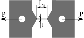
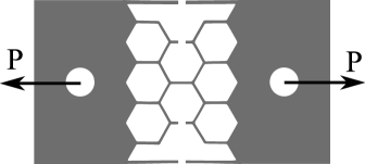
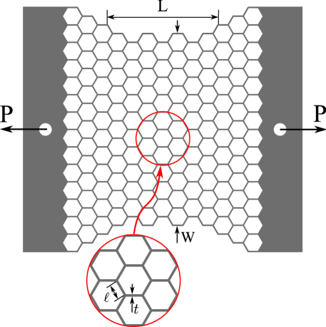
Figure 1: LABEL:sub@fig:dbTension Macroscale dogbone-shaped specimen, LABEL:sub@fig:singleStrutTension single strut specimen, LABEL:sub@fig:singleStrut unit cell test specimen, and LABEL:sub@fig:PerfectLatticeSketch regular lattice specimen of $\mkern 1.25mu\overline{\mkern-1.25mu\rho\mkern-1.25mu}\mkern 1.25mu=0.11$. The sheet thickness of all samples is $B_{0}=$5\text{\,}\mathrm{m}\mathrm{m}$$.

A regular two-dimensional (2D) hexagonal lattice is shown in Fig. 1. It comprises struts of length $\ell$ and in-plane thickness $t$ such that the relative density of the lattice is given by [13]

$$\overline{\rho}=\frac{2}{\sqrt{3}}\frac{t}{\leavevmode\hbox{\set@color$\ell$}}$$ (1)

for $t/\leavevmode\hbox{\set@color$\ell$}<0.2$. Under macroscopic uniaxial tensile loading, the hexagonal lattice is bending-dominated in its small strain elastic response due to low nodal connectivity of 3, see for example [13]. However, at a sufficiently high value of tensile macroscopic strain, the response of the lattice switches from a compliant, bending-dominated mode to a stiff, stretching-dominated mode as the cell walls align with the tensile direction [14, 18]. In general, the uniaxial tensile response of an elastoplastic hexagonal lattice proceeds in 4 stages under an increasing macroscopic strain, as discussed by Ronan et al. [14]: (i) elastic bending of the struts inclined to the loading axis, (ii) plastic bending, (iii) elastic stretching of all struts in the lattice as the inclined struts align with the loading direction, and (iv) plastic stretching. Failure may intervene during any of these 4 regimes depending upon the active mode of cell wall failure. Tankasala et al. [18] have assumed 2 possible criteria for the failure of a cell wall: (i) when the maximum local strain at any point in the lattice attains the failure strain of the solid; this criterion is appropriate for lattices made from ceramics and brittle alloys, or (ii) when the maximum value of average tensile strain across any cell wall of the lattice attains the cell wall failure strain; this criterion is suitable for ductile alloys which undergo necking, see for example Onck et al. [23]. The wide range in the mechanical response of the hexagonal lattice (depending upon the cell wall material) motivates its choice in the present study. We choose polymethyl methacrylate (PMMA) for the cell wall material as it is elastic-brittle at room temperature, but exhibits a strong visco-plastic characteristic at temperatures close to the glass transition value. The creep response of PMMA lattices at high temperature is the subject of a follow-on study.

1.3 Scope of study

The purpose of the current study is to examine experimentally the tensile response of two-dimensional (2D) elastic-brittle lattice materials made by rapid prototyping. Lattices were cut from polymethyl methacrylate (PMMA) sheets and were tested under uniaxial tension at room temperature. The sensitivity of the macroscopic tensile stress versus strain curve to as-manufacturing defects, such as variations in strut thickness and Plateau border radius, was determined for regular hexagonal lattices. Finite element (FE) calculations were used to assess the significance of as-manufactured defects on the macroscopic properties; the precise lattice geometry was determined by computer-assisted tomography (CT). Irregular lattices were also created by the introduction of as-designed defects, specifically a centre crack (due to missing cell walls), solid inclusions in the form of filled cells, and randomly perturbed joints. The knockdown in lattice strength due to each of these defects was measured.

2 Experimental programme

Specimens were manufactured by the laser-cutting of cast $5\text{\,}\mathrm{m}\mathrm{m}$ thick PMMA sheets into the following 5 geometries:

• macroscale, dogbone-shaped specimen, as shown in Fig. 1, for material characterisation on a large scale;

• single strut specimen, as shown in Fig. 1, for material characterisation on a small scale;

• unit cell specimen of the lattice, comprising a single strut embedded in hexagonal cells, see Fig. 1;

• regular hexagonal lattice, as shown in Fig. 1, to measure the lattice response, absent as-designed defects;

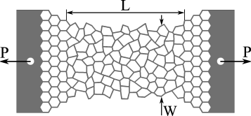
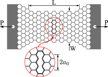
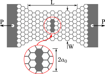
Figure 2: Lattice specimens ($\mkern 1.25mu\overline{\mkern-1.25mu\rho\mkern-1.25mu}\mkern 1.25mu=0.11$, gauge width $W$ of 7 cells, and gauge length $L$ of 13 cells) containing as-designed defects in the form of LABEL:sub@fig:Model_Seed1_0_Radius0_5 randomly perturbed joints ($R/\leavevmode\hbox{\set@color$\ell$}=0.5$), LABEL:sub@fig:RemovedCellWallsSketch a row of missing cell walls, and LABEL:sub@fig:FilledCellsSketch a row of solid inclusions.

• irregular hexagonal lattice containing as-designed defects in the form of (a) randomly perturbed joints, (b) missing cell walls, or (c) solid inclusions, see Fig. 2.

The strut thickness in specimens of type (ii) to (iv) is $t=$0.47\text{\,}\mathrm{m}\mathrm{m}$$. For lattice specimens of type (iv), the relative density of the lattice $\mkern 1.25mu\overline{\mkern-1.25mu\rho\mkern-1.25mu}\mkern 1.25mu$ is varied from 0.07 to 0.19 by varying strut length $\ell$ in the range of $3.0\text{\,}\mathrm{m}\mathrm{m}$ to $7.5\text{\,}\mathrm{m}\mathrm{m}$, as demanded by Eq. (1). The PMMA material employed in this study has a glass transition temperature $T_{\mathrm{g}}=$385\text{\,}\mathrm{K}$$. All specimens were tested at room temperature $T=$296\text{\,}\mathrm{K}$=0.77T_{\mathrm{g}}$.

2.1 Manufacture of regular hexagonal lattices

A computer-aided drawing (CAD) of the geometry of a regular hexagonal lattice, as shown in Fig. 1, was created using the OpenSCAD software. This CAD file provides an input to the laser cutting machine with sufficient data to define the translation of the cutting head relative to a fixed position on the PMMA sheet. The hexagonal lattices were manufactured to a dogbone shape in order to ensure that failure occurs within the gauge section, see Fig. 1. All regular lattice specimens have a gauge width $W=11\sqrt{3}\leavevmode\hbox{\set@color$\ell$}$ (or 11 cells) and a gauge length $L=11\leavevmode\hbox{\set@color$\ell$}$ (or 7 cells). (The same sample size of $11\,\times\,7$ cells in the gauge area was used in the follow-on study at elevated temperature.)

2.2 Test method

All lattices were tested in uniaxial tension using a screw-driven test machine at a nominal strain rate of $\dot{\varepsilon}=$3.6\text{\times}{10}^{-4}\text{\,}\mathrm{s}^{-1}$$. The load $P$ is measured via a load cell clamped to the stationary platen of the rig while the extension $u$ of the gauge length is determined by Digital Image Correlation (DIC), as follows. Prior to the start of the test, the lattice specimens were coated with a thin layer of white chalk and a speckle pattern was then generated by spraying black paint in order to enhance the contrast of the DIC imagery. A single camera of the GOM ARAMIS 12M system was used to track facets of size $20\,\times\,20$ pixels in the vicinity of a predefined node at the top and bottom of the gauge length. This procedure enabled the sub-pixel resolution of the nodal displacements.

The uniaxial tensile response of the solid was measured by testing two geometries: (i) dogbone-shaped solid specimens (of cross-sectional dimensions $$10\text{\,}\mathrm{m}\mathrm{m}$\,\times\,$5\text{\,}\mathrm{m}\mathrm{m}$$ and gauge length $L_{\mathrm{d}}=$80\text{\,}\mathrm{m}\mathrm{m}$$) and (ii) single strut specimens (of mean strut thickness $\mkern 1.25mu\overline{\mkern-1.25mut\mkern-1.25mu}\mkern 1.25mu=$0.47\text{\,}\mathrm{m}\mathrm{m}$$ and strut length $L_{\mathrm{s}}=$10\text{\,}\mathrm{m}\mathrm{m}$$). The extension of the gauge length of the large dogbone specimens was measured by a non-contact laser extensometer while that of single strut specimens was measured by optical tracking of white dots marked on the top and the bottom of the gauge length along the centre-line of the specimen. The dogbone-shaped specimens were gripped by wedge grips and the single strut specimens were pin-loaded.

3 Material characterisation

3.1 Strut geometry

Geometrical features such as the thickness and Plateau border radius of the individual struts of the laser-cut lattice were measured using computer-assisted X-ray tomography. A probability density function of the strut thickness $t$ was generated by measuring its value at mid-length on 453 struts of a regular honeycomb lattice of $\mkern 1.25mu\overline{\mkern-1.25mu\rho\mkern-1.25mu}\mkern 1.25mu=0.11$ via image processing of its CT scan. The strut thickness follows a normal distribution with a mean value $\mkern 1.25mu\overline{\mkern-1.25mut\mkern-1.25mu}\mkern 1.25mu=$0.47\text{\,}\mathrm{m}\mathrm{m}$$ and a standard deviation $t_{\rm sd}=$0.09\text{\,}\mathrm{m}\mathrm{m}$$ and this is expressed via the notation $t=0.47\pm$0.09\text{\,}\mathrm{m}\mathrm{m}$$. We emphasise that the same notation is used to give the mean value and standard deviation of other quantities such as peak load, stress and so on. The as-manufactured lattice specimens also possess a dispersion in the Plateau border radius of each joint. To quantify this distribution, values of the Plateau border radius were measured at 300 locations across 10 unit cell specimens; the smaller size of the unit cell specimens ensured higher spatial resolution of their CT scans. The Plateau borders have a mean radius of $\mkern 1.25mu\overline{\mkern-1.25mur\mkern-1.25mu}\mkern 1.25mu=$0.4\text{\,}\mathrm{m}\mathrm{m}$$ and a standard deviation $r_{\rm sd}=$0.1\text{\,}\mathrm{m}\mathrm{m}$$ (not shown).

3.2 Solid material response

The as-manufactured material properties of solid PMMA were measured from the response of a large dogbone-shaped specimen and of a single strut of the lattice; any size effect on the properties is thereby determined. The nominal stress versus strain response of the solid dogbone specimens and single strut specimens are compared in Fig. 3. All specimens respond in an elastic-brittle manner. The Young’s modulus of the solid material, as measured from the dogbone specimens, is $E_{\mathrm{s}}=2.5\pm$0.2\text{\,}\mathrm{G}\mathrm{P}\mathrm{a}$$, and the tensile strength is $\sigma_{\mathrm{fs}}=63\pm$2\text{\,}\mathrm{M}\mathrm{P}\mathrm{a}$$. In contrast, the Young’s modulus and tensile strength of the solid material, as measured from the single strut experiments, is $E_{\mathrm{s}}=2.4\pm$0.3\text{\,}\mathrm{G}\mathrm{P}\mathrm{a}$$ and $\sigma_{\mathrm{fs}}=36\pm$14\text{\,}\mathrm{M}\mathrm{P}\mathrm{a}$$. Whilst the value of Young’s modulus is comparable for the two geometries, the tensile strength of the single strut is less than that of the larger specimens by approximately 40%. This is ascribed to the difference in thermal histories during manufacture. A significant scatter in the macroscopic failure strain is also observed for the single strut specimens, such that the ductility $\varepsilon_{\mathrm{fs}}=0.015\pm 0.007$.

4 Numerical study

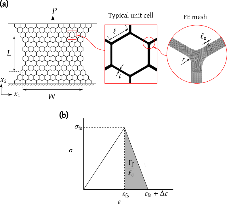
Figure 4: Details of the FE model: (a) geometry, loading, and boundary conditions employed in the FE simulations of lattice specimens under uniaxial tension. A typical unit cell within the lattice is shown along with the FE mesh for a joint. (b) Assumed stress versus strain response of the cell wall solid.

Quasi-static FE simulations were performed using ABAQUS/Explicit v6.14 to simulate the observed response of the hexagonal lattices under uniaxial tension. The 2D geometry for each FE model is defined from the CT scan at the mid-plane of the corresponding as-manufactured 3D specimen. Uniaxial loading of the lattice is simulated by constraining all degrees of freedom along the bottom edge of the specimen while the top edge is subjected to uniform displacement in the $x_{2}$-direction of the specimen, see Fig. 4 ​(a). The as-manufactured lattice of Fig. 4 contains 453 struts, each of length $\leavevmode\hbox{\set@color$\ell$}\approx$5\text{\,}\mathrm{m}\mathrm{m}$$. A typical unit cell within the lattice is shown in the inset of Fig. 4 ​(a): the struts within the lattice have variable thickness and variable Plateau border radius due to the manufacturing process. The FE mesh of the lattice comprises triangular elements with quadratic shape functions and in-plane strain (type CPE6M). The elements are of uniform size $\leavevmode\hbox{\set@color$\ell$}_{\rm e}$, chosen to be such that the thinnest strut in the lattice has at least 7 elements across its thickness, and the stress concentration at the Plateau borders is adequately captured. A typical FE mesh at a joint in the lattice is shown in Fig. 4 ​(a).

The assumed stress $\sigma$ versus strain $\varepsilon$ response of the cell wall solid is sketched in Fig. 4 ​(b). A continuum damage model is employed in the FE calculations to simulate fracture of any element. The overall response of a material point (i.e. at each integration point of an element) proceeds in 3 stages as follows:

• The initial undamaged response is linear elastic with Young’s modulus ${E}_{\rm s}=$2.4\text{\,}\mathrm{G}\mathrm{P}\mathrm{a}$$, as taken from the measured mean value of single strut specimens, recall Section 3.2. A Poisson’s ratio of $\nu_{\rm s}=0.3$ is assumed for the cell wall solid.

• Failure initiates at an integration point when the maximum tensile stress at that point attains the solid tensile strength, $\sigma_{\rm fs}$, as indicated in Fig. 4 ​(b). A deterministic value of $\sigma_{\rm fs}=$36\text{\,}\mathrm{M}\mathrm{P}\mathrm{a}$$ is assumed for all struts in the lattice, as taken from the measured mean tensile strength of single strut specimens, recall Section 3.2.

• The subsequent evolution of damage at a material point is specified via a linear softening $\sigma$ versus $\varepsilon$ response in accordance with a specified fracture energy $\Gamma_{\rm f}$ as defined by

  $$\Gamma_{\rm f}=\leavevmode\hbox{\set@color$\ell$}_{\rm c}\int_{\varepsilon_{\rm fs}}^{\varepsilon_{\rm fs}+\Delta\varepsilon}\sigma\;d\varepsilon$$ (2)

  where $\leavevmode\hbox{\set@color$\ell$}_{\rm c}$ is a characteristic length associated with the integration point of the element: $\leavevmode\hbox{\set@color$\ell$}_{\rm c}$ equals $\leavevmode\hbox{\set@color$\ell$}_{\rm e}/2$ for quadratic triangular finite elements, $\varepsilon_{\rm fs}$ equals $\sigma_{\rm fs}/E_{\rm s}$, and $\Delta\varepsilon$ is the strain increment over the softening portion of the response, see Fig. 4 ​(b). A triangular damage evolution law is assumed in the present study such that $\Delta\varepsilon=2\Gamma_{\rm f}/\sigma_{\rm fs}\leavevmode\hbox{\set@color$\ell$}_{\rm c}$. Note that there is choice in the precise value of $\Gamma_{\rm f}$; the FE simulations reported here assume $\Gamma_{\rm f}=0.1\ \rm kJ/m^{2}$ following [25]. It is noted that the specification of damage evolution via Eq. (2) in terms of the size of the finite element alleviates the problem of mesh dependence of the solution; refer to [26] for details.

5 Tensile response of as-manufactured lattice specimens: prediction versus experiment

The measured tensile response of the two geometries of specimens, the unit cell specimen of Fig. 1 and the lattice specimen of Fig. 1, are discussed in turn. Comparisons with the FE predictions are made alongside.

5.1 Unit cell specimen

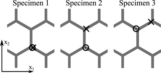
Figure 5: Measured (Exp.) and predicted (FE) responses for 3 as-manufactured unit cell specimens with $t/\leavevmode\hbox{\set@color$\ell$}=0.1$. LABEL:sub@fig:fe_pu_singlestrut Load versus displacement response until first strut failure, and LABEL:sub@fig:fe_failure_singlestrut location of first strut failure for the three specimens; the circles indicate observed failure sites while the crosses indicate predicted failure sites.

Consider the unit cell specimen of Fig. 1. We characterise the structural response of this specimen in terms of its load $P$ versus overall displacement $u$, and include the as-manufactured defects in the FE predictions of the structural response. In the experiments, two support struts, spanning the height of the specimen on either side of the central strut, protect the specimen prior to the test; these are cut at their mid-length immediately prior to the test. A total of 10 specimens were tested under uniaxial tension along the axis of the central strut, see Fig. 1. All struts are of length $\leavevmode\hbox{\set@color$\ell$}=$5\text{\,}\mathrm{m}\mathrm{m}$$ and the mean thickness of a strut (across the 10 specimens) is $\mkern 1.25mu\overline{\mkern-1.25mut\mkern-1.25mu}\mkern 1.25mu=$0.47\text{\,}\mathrm{m}\mathrm{m}$$. The measured load $P$ versus displacement $u$ response of 3 representative unit cell specimens is shown in Fig. 5. In each case, the response is shown until failure of the first strut. The peak load is $P_{\mathrm{max}}=28.6\pm$5.4\text{\,}\mathrm{N}$$ from the measured values of 10 specimens. Failure of all specimens (except one) occurs in an inclined strut adjacent to the central vertical strut and close to the joint.

FE predictions of the tensile response of 3 unit cell specimens are included in Fig. 5; the 2D geometry of each specimen is determined from a CT scan of the mid-plane of the corresponding as-manufactured specimen. A constant value of strut tensile strength, $\sigma_{\rm fs}=$36\text{\,}\mathrm{M}\mathrm{P}\mathrm{a}$$, is assumed for all struts in the specimen, as taken from the mean value of the measured tensile strength of the single strut specimens, recall Section 3.2. We find from Fig. 5 that the predicted $P$ versus $u$ response is consistent with the measured response for specimens 1 and 2, indicating that the dispersion in geometry (i. e. variation in strut thickness and Plateau border radius) largely explains the observed response of the unit cell specimens. The strut tensile strength is likely to be uniform in the unit cell specimens for the following reason. The variance in the strut strength is a consequence of thermal history associated with strut manufacture. The time interval between laser-cutting of the first and the last struts of the specimen is only 20 seconds for the unit cell specimens and consequently, there is good repeatability in strength from strut to strut. Agreement is less satisfactory for specimen 3, for reasons unknown. The location of first strut failure, as seen in the 3 representative specimens, is sketched in Fig. 5: the circles denote the location of first strut failure in experiments while crosses are the FE predictions. A single strut in the FE simulation is considered to have failed when a row of finite elements at any strut cross-section become stress-free, following Eq. (2). In general, the critical strut that fails first is an inclined strut adjacent to the central vertical strut, in both experiments and FE.

Both experiments and FE reveal that failure occurs within the inclined struts at a location near the joints. Thus, the FE indicates that the local stress in the inclined struts exceeds that of the central strut.

5.2 Lattice specimens

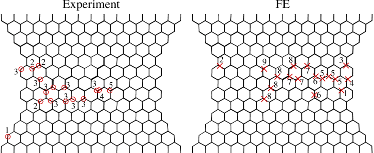
Figure 6: Comparison of the measured and FE responses for lattice specimens of $\mkern 1.25mu\overline{\mkern-1.25mu\rho\mkern-1.25mu}\mkern 1.25mu=0.11$. LABEL:sub@fig:fe_exp_stressstrain_47 Stress versus strain response, and LABEL:sub@fig:fe_failure_lattice_caseE sequence of strut failure for one realisation (Test I). The crosses and circles indicate the location of failure and the number denotes its position in the failure sequence. The macroscopic stress at first strut failure and the peak stress of five measured specimens are compared with FE predictions in LABEL:sub@fig:fe_exp_stresses_mod along with Test I.

The measured macroscopic nominal stress $\sigma^{\infty}$ versus nominal strain $\varepsilon^{\infty}$ response of one lattice specimen (labelled Test I) of relative density $\mkern 1.25mu\overline{\mkern-1.25mu\rho\mkern-1.25mu}\mkern 1.25mu=0.11$ is shown in Fig. 6, with $\sigma^{\infty}$ and $\varepsilon^{\infty}$ defined in terms of the reaction force $P$ on the top edge and the extension $u$ of the gauge length as $\sigma^{\infty}=P/(WB_{0})$ and $\varepsilon^{\infty}=u/L$, respectively. The gauge dimensions $(W,L)$ are indicated in Fig. 4; $W=$95.3\text{\,}\mathrm{m}\mathrm{m}$$, $L=$55\text{\,}\mathrm{m}\mathrm{m}$$, and $B_{0}=$5\text{\,}\mathrm{m}\mathrm{m}$$ for the specimen of Fig. 6. The FE prediction of the macroscopic response is included in Fig. 6. As before, the geometry of the FE model is determined from a CT scan of the mid-plane of the as-manufactured specimen. A constant tensile strength of $\sigma_{\rm fs}=$36\text{\,}\mathrm{M}\mathrm{P}\mathrm{a}$$ is assumed for all struts in the lattice, as taken from the mean value of the measured tensile strength of the single strut specimens in Section 3.2. The sequence of strut failure is shown in Fig. 6 for both measurement and prediction: the number indicates the position of struts in the failure sequence with their actual location marked in Fig. 6. We find from Fig. 6 and Fig. 6 that an initial drop in load accompanies failure of a strut located at the edge of the specimen. Subsequent load drops correspond to the simultaneous failure of multiple struts in the vicinity of previously failed struts. Eventually, a dominant macroscopic crack propagates across the specimen leading to catastrophic fracture. The FE predictions for the initial stiffness and the load corresponding to first strut failure are in close agreement with the corresponding values in the experiment, despite the mismatch in the precise location of strut failure, see Fig. 6 and Fig. 6.

Additional tension tests were performed on 4 lattice specimens (also of $\mkern 1.25mu\overline{\mkern-1.25mu\rho\mkern-1.25mu}\mkern 1.25mu=0.11$). The measured and predicted values of the macroscopic stress corresponding to the first strut failure, and the peak stress are shown in Fig. 6 for all 5 lattice specimens. In all cases, failure of the lattice occurs in a correlated manner (i. e. via the formation of a single horizontal crack originating from one edge of the specimen) subsequent to first strut failure. FE simulations of the 4 specimens also predict this pattern of failure. Visual examination of the failed specimens further revealed that the struts always fail close to a joint, and that the thinner struts fail first: the mean thickness of failed struts is about 10% lower than the overall mean strut thickness of $0.47\text{\,}\mathrm{m}\mathrm{m}$.

5.3 Effect of relative density on the macroscopic properties

It is instructive to evaluate the accuracy of the scaling laws for the Young’s modulus and tensile strength of a lattice material of infinite extent with those of the laser-cut finite specimens of the present study. Consider a regular hexagonal lattice comprising struts of length $\ell$ and thickness $t$, and made from an elastic-brittle solid of Young’s modulus $E_{\mathrm{s}}$ and tensile strength $\sigma_{\mathrm{fs}}$. The macroscopic in-plane modulus $E$ and tensile strength ${\sigma^{\infty}_{\mathrm{f}}}$ of an infinite hexagonal lattice are given by [13]

$${E}=\dfrac{3}{2}\mkern 1.25mu\overline{\mkern-1.25mu\rho\mkern-1.25mu}\mkern 1.25mu^{3}E_{\mathrm{s}}\quad\textrm{and}\quad{\sigma^{\infty}_{\mathrm{f}}}=\dfrac{1}{3}\mkern 1.25mu\overline{\mkern-1.25mu\rho\mkern-1.25mu}\mkern 1.25mu^{2}{\sigma_{\mathrm{fs}}}$$ (3)

Lattice specimens of geometry identical to those as shown in Fig. 1 were laser-cut from PMMA sheets, in order to verify the accuracy of Eq. (3) as a function of the relative density of the lattice. In each case, the strut thickness $t$ was held constant such that $\mkern 1.25mu\overline{\mkern-1.25mut\mkern-1.25mu}\mkern 1.25mu=$0.47\text{\,}\mathrm{m}\mathrm{m}$$ for all struts, and the strut length $\ell$ was varied in accordance with Eq. (1) to generate lattices of $\mkern 1.25mu\overline{\mkern-1.25mu\rho\mkern-1.25mu}\mkern 1.25mu=0.07$ and $\mkern 1.25mu\overline{\mkern-1.25mu\rho\mkern-1.25mu}\mkern 1.25mu=0.19$.

The measured values of macroscopic modulus $E$ and tensile strength $\sigma^{\infty}_{\mathrm{f}}$ of the lattice specimens are plotted in Fig. 7 as a function of $\mkern 1.25mu\overline{\mkern-1.25mu\rho\mkern-1.25mu}\mkern 1.25mu$ for 5 specimens per value of $\mkern 1.25mu\overline{\mkern-1.25mu\rho\mkern-1.25mu}\mkern 1.25mu$, upon normalising $E$ and $\sigma_{\mathrm{f}}^{\infty}$ by $\mkern 1.25mu\overline{\mkern-1.25muE\mkern-1.25mu}\mkern 1.25mu_{\mathrm{s}}=$2.5\text{\,}\mathrm{G}\mathrm{P}\mathrm{a}$$ and $\mkern 1.25mu\overline{\mkern-1.25mu\sigma\mkern-1.25mu}\mkern 1.25mu_{\mathrm{fs}}=$36\text{\,}\mathrm{M}\mathrm{P}\mathrm{a}$$ , respectively. The predictions of Eq. (3) are included in Fig. 7 for comparison. It is clear that both $E$ and $\sigma^{\infty}_{\mathrm{f}}$ scale with $\mkern 1.25mu\overline{\mkern-1.25mu\rho\mkern-1.25mu}\mkern 1.25mu$ according to Eq. (3). Deviation of the measured values of $E$ and $\sigma^{\infty}_{\mathrm{f}}$ from Eq. (3), and the scatter in data for each value of $\mkern 1.25mu\overline{\mkern-1.25mu\rho\mkern-1.25mu}\mkern 1.25mu$ are attributed to the as-manufactured defects such as the variation in strut thickness $t$ and variation of Plateau border $r$ in addition to the finite size of the specimen. The measured values of the macroscopic Young’s modulus and the macroscopic tensile strength as obtained from dogbone specimens, with a gauge size of 13 cells (in height) and 7 cells (in width), are included in Fig. 7 along with the case of 11 $\times$ 7 cells for lattices of $\mkern 1.25mu\overline{\mkern-1.25mu\rho\mkern-1.25mu}\mkern 1.25mu=0.11$. The observed insensitivity of the macroscopic elastic response with choice of specimen geometry, as seen in Fig. 7, is consistent with the fact that the elastic boundary layer in a hexagonal lattice spans only one cell size.

It remains to determine by FE analysis the explicit role of each type of as-manufactured defect in reducing the macroscopic tensile strength. We achieve this by the sequential introduction of two classes of geometric imperfections, (i) a dispersion in strut thickness and (ii) a dispersion in Plateau border. The details are as follows.

6 Effect of as-manufactured defects upon the macroscopic tensile strength: prediction versus experiment

The role of geometric imperfections, such as a dispersion in strut thickness and in Plateau border radius, is now predicted by considering the following lattice geometries, with the salient details of each geometry as summarised in Table 1.

• Case A is the reference case of a geometrically perfect lattice with a deterministic, uniform value of strut thickness $t=\mkern 1.25mu\overline{\mkern-1.25mut\mkern-1.25mu}\mkern 1.25mu=$0.47\text{\,}\mathrm{m}\mathrm{m}$$ and of Plateau border radius $r=\mkern 1.25mu\overline{\mkern-1.25mur\mkern-1.25mu}\mkern 1.25mu=$0.4\text{\,}\mathrm{m}\mathrm{m}$$.

• Case B is an imperfect lattice, with a normal distribution of the Plateau border radius such that the mean radius in the specimen is $\mkern 1.25mu\overline{\mkern-1.25mur\mkern-1.25mu}\mkern 1.25mu=$0.4\text{\,}\mathrm{m}\mathrm{m}$$ and standard deviation $r_{\rm sd}/\mkern 1.25mu\overline{\mkern-1.25mur\mkern-1.25mu}\mkern 1.25mu=0.25$, based on measurements of the as-manufactured specimens, as discussed previously in Section 3.1. All struts of this geometry have a constant value of strut thickness $t=\mkern 1.25mu\overline{\mkern-1.25mut\mkern-1.25mu}\mkern 1.25mu=$0.47\text{\,}\mathrm{m}\mathrm{m}$$, as for case A.

• Case C is an imperfect lattice, with a normal distribution of the strut thickness such that $\mkern 1.25mu\overline{\mkern-1.25mut\mkern-1.25mu}\mkern 1.25mu=$0.47\text{\,}\mathrm{m}\mathrm{m}$$ and $t_{\rm sd}/\mkern 1.25mu\overline{\mkern-1.25mut\mkern-1.25mu}\mkern 1.25mu=0.19$, based on measurements of the as-manufactured specimens of Section 3.1. All struts of this geometry have a constant value of Plateau border radius $r=\mkern 1.25mu\overline{\mkern-1.25mur\mkern-1.25mu}\mkern 1.25mu=$0.4\text{\,}\mathrm{m}\mathrm{m}$$, as for case A.

• Case D is an imperfect lattice, with a normal distribution of both the strut thickness and the Plateau border radius such that $\mkern 1.25mu\overline{\mkern-1.25mut\mkern-1.25mu}\mkern 1.25mu=$0.47\text{\,}\mathrm{m}\mathrm{m}$$, $\mkern 1.25mu\overline{\mkern-1.25mur\mkern-1.25mu}\mkern 1.25mu=$0.4\text{\,}\mathrm{m}\mathrm{m}$$, $t_{\rm sd}/\mkern 1.25mu\overline{\mkern-1.25mut\mkern-1.25mu}\mkern 1.25mu=0.19$, and $r_{\rm sd}/\mkern 1.25mu\overline{\mkern-1.25mur\mkern-1.25mu}\mkern 1.25mu=0.25$. All struts have a uniform thickness along their length.

• Case E is a set of nominally identical as-manufactured geometries. Each is defined from a CT scan of the mid-plane section of the corresponding as-manufactured lattice specimen, as previously discussed in Section 5.2. We emphasise that each as-manufactured geometry contains imperfections resulting from the manufacturing process (such as wavy or misaligned struts, and non-uniform thickness along the strut length). The distribution of strut thickness and Plateau border radius for this set of as-manufactured geometries has already been characterised as $\mkern 1.25mu\overline{\mkern-1.25mut\mkern-1.25mu}\mkern 1.25mu=$0.47\text{\,}\mathrm{m}\mathrm{m}$$, $\mkern 1.25mu\overline{\mkern-1.25mur\mkern-1.25mu}\mkern 1.25mu=$0.4\text{\,}\mathrm{m}\mathrm{m}$$, $t_{\rm sd}/\mkern 1.25mu\overline{\mkern-1.25mut\mkern-1.25mu}\mkern 1.25mu=0.19$, and $r_{\rm sd}/\mkern 1.25mu\overline{\mkern-1.25mur\mkern-1.25mu}\mkern 1.25mu=0.25$ in Section 3.1.

In all cases, the strut length equals $\leavevmode\hbox{\set@color$\ell$}=$5\text{\,}\mathrm{m}\mathrm{m}$$ such that $\mkern 1.25mu\overline{\mkern-1.25mu\rho\mkern-1.25mu}\mkern 1.25mu=0.11$, and a constant value of strut tensile strength is assumed such that $\sigma_{\rm fs}=$36\text{\,}\mathrm{M}\mathrm{P}\mathrm{a}$$. The FE predictions of the lattice tensile strength $\sigma^{\infty}_{\rm f}$ (based on failure of the first strut) are listed in Table 1 for cases A to D; data are presented in terms of the mean strength $\mkern 1.25mu\overline{\mkern-1.25mu\sigma\mkern-1.25mu}\mkern 1.25mu^{\infty}_{\rm f}$ and standard deviation ${\sigma}^{\infty}_{\rm f,sd}$ from 10 realisations. The values in each case are normalised by the mean measured strength of the lattice, $\mkern 1.25mu\overline{\mkern-1.25mu\sigma\mkern-1.25mu}\mkern 1.25mu^{\infty}_{\rm Exp}$. The predicted values of tensile strength for 5 realisations of case E are included in Table 1 for comparison. It is clear from Table 1 that the introduction of geometric imperfection reduces the mean value of the macroscopic tensile strength: a dispersion in thickness alone (case C) reduces the tensile strength by up to $20\%$ compared to that of the perfect lattice strength (case A). An additional dispersion in Plateau border radius (case D) only slightly reduces the mean value of the tensile strength, but it increases the scatter in strength, compare cases B and D in Table 1. We conclude from Table 1 that dispersion in strut thickness is the primary source of the reduction in the mean tensile strength of laser-cut PMMA lattices.

6.1 Dispersion in strut tensile strength

It is evident from Table 1 that the scatter in ${\sigma}^{\infty}_{\rm f}$ for the as-manufactured lattices (case E, Exp.) is under-predicted in the FE simulations (case E). Assuming that the geometrical as-manufactured imperfections are accurately captured by the FE simulations, a probable source of the observed scatter in ${\sigma}^{\infty}_{\rm f}$ for case E experiments is the variation in tensile strength of the strut material in the lattice, which is a consequence of the thermal history imposed by the laser-cutting process. To assess the role of strength dispersion, FE simulations were performed on 10 realisations of a geometrically perfect lattice (case A) and for an assumed distribution of strut tensile strength of mean value $\mkern 1.25mu\overline{\mkern-1.25mu\sigma\mkern-1.25mu}\mkern 1.25mu_{\rm fs}=$36\text{\,}\mathrm{M}\mathrm{P}\mathrm{a}$$. Two choices of standard deviation of the distribution of strut strength were assumed: $\sigma_{\rm fs,sd}/\mkern 1.25mu\overline{\mkern-1.25mu\sigma\mkern-1.25mu}\mkern 1.25mu_{\rm fs}=0.1$ and $0.2$. The normal distribution curve of strut strength in each case is truncated such that the strut strength in the lattice varies from $22\text{\,}\mathrm{M}\mathrm{P}\mathrm{a}$ to $50\text{\,}\mathrm{M}\mathrm{P}\mathrm{a}$, based on the observed minimum and maximum strut tensile strength, respectively, from the single strut tests (recall Section 3.2). The resulting probability density functions of strut strength are shown in Fig. 8 for $\sigma_{\rm fs,sd}/\mkern 1.25mu\overline{\mkern-1.25mu\sigma\mkern-1.25mu}\mkern 1.25mu_{\rm fs}=0.1$ and $0.2$.

The FE predictions of the normalised macroscopic tensile strength for 10 realisations are plotted in Fig. 8 for the two selected values of $\sigma_{\rm fs,sd}/\mkern 1.25mu\overline{\mkern-1.25mu\sigma\mkern-1.25mu}\mkern 1.25mu_{\rm fs}$. The dispersion in the strut tensile strength leads to a significant reduction in the mean value of the tensile strength by up to $20\%$ (for $\sigma_{\rm fs,sd}/\mkern 1.25mu\overline{\mkern-1.25mu\sigma\mkern-1.25mu}\mkern 1.25mu_{\rm fs}=0.2$) but only mildly increases the scatter. We conclude from Table 1 and Fig. 8 that the dispersion in strut thickness and in strut tensile strength are each potent sources of knockdown in the macroscopic strength of the as-manufactured PMMA lattices.

7 The effect of as-designed defects on macroscopic tensile strength

Three types of macroscopic defect were introduced within the regular lattice by design: (i) misplaced joints, (ii) cells filled with solid inclusions, and (iii) missing cell walls. The resulting as-manufactured specimens contain geometric imperfections at the cell wall level (variation in strut thickness and Plateau border radius) in addition to one of the three macroscopic defects, see Fig. 2. The macroscopic tensile strength of the as-manufactured specimens was measured experimentally and then compared with that of the as-manufactured topologies designed without macroscopic defects. The sensitivity of measured tensile strength to the presence of as-designed defects was thereby assessed.

7.1 Randomly perturbed joints

Imperfect hexagonal lattices were manufactured by first generating a CAD file of a lattice with randomly perturbed joints. To achieve this, the joints of a regular hexagonal lattice (of $\mkern 1.25mu\overline{\mkern-1.25mu\rho\mkern-1.25mu}\mkern 1.25mu=0.11$) were repositioned randomly within a circular disc of radius $R$, following the procedure as used by Romijn and Fleck [20]. The degree of imperfection was varied by selecting values of $R/\leavevmode\hbox{\set@color$\ell$}$ between $0$ ( regular lattice) and $0.5$ (extremely imperfect lattice). A typical realisation of the as-manufactured lattice, for the choice $R/\leavevmode\hbox{\set@color$\ell$}=0.5$, is shown in Fig. 2; only those joints which lie within the gauge section are misplaced. The random misplacement of the joints reduces the average strut length such that the relative density of the lattice increases by a factor of 1.0025 for $R/\leavevmode\hbox{\set@color$\ell$}=0.1$ and by a factor of 1.0625 for $R/\leavevmode\hbox{\set@color$\ell$}=0.5$, as previously noted by Romijn and Fleck [20]; this minor change in $\mkern 1.25mu\overline{\mkern-1.25mu\rho\mkern-1.25mu}\mkern 1.25mu$ is ignored in the current study.

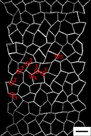
Figure 9: LABEL:sub@fig:misplacedNodes_AllRTE Measured macroscopic properties of imperfect lattices with randomly misplaced joints: normalised Young’s modulus $\hat{E}$, normalised tensile strength $\hat{\sigma}$, and Poisson’s ratio $\nu$. LABEL:sub@fig:hexlattice_cut_26_failure Sequence of strut failure for one specimen of $R/\leavevmode\hbox{\set@color$\ell$}=0.5$. The scale bar is of length $10\text{\,}\mathrm{m}\mathrm{m}$.

The sensitivity to random perturbation of joints is measured for 3 macroscopic properties of the imperfect lattice: (i) Young’s modulus $E$, (ii) Poisson’s ratio $\nu$, and (iii) tensile strength $\sigma^{\infty}_{\mathrm{f}}$. These observed sensitivities are plotted in Fig. 9 as a function of the degree of imperfection $R/\leavevmode\hbox{\set@color$\ell$}$, for the choice of $\mkern 1.25mu\overline{\mkern-1.25mu\rho\mkern-1.25mu}\mkern 1.25mu=0.11$. The ordinate in each case (except for $\nu$) is normalised by its corresponding mean value as measured for the regular lattice ($R/\leavevmode\hbox{\set@color$\ell$}=0$). Results are shown for 3 realisations of imperfect lattice for each choice of $R/\leavevmode\hbox{\set@color$\ell$}=0,0.3,$ and $0.5$. The Young’s modulus $E$ of the imperfect lattice increases with increasing $R/\leavevmode\hbox{\set@color$\ell$}$ as previously noted by Ronan et al. [14]: the mean value of $E$ increases by 45% for $R/\leavevmode\hbox{\set@color$\ell$}=0.3$, and by 50% for $R/\leavevmode\hbox{\set@color$\ell$}=0.5$, compared to its value at $R/\leavevmode\hbox{\set@color$\ell$}=0$. The observed reduction of $\nu$ with increasing $R/\leavevmode\hbox{\set@color$\ell$}$ supports the prediction of Romijn and Fleck [20] (not shown). The macroscopic tensile strength $\sigma^{\infty}_{\mathrm{f}}$ is almost insensitive to the value of $R/\leavevmode\hbox{\set@color$\ell$}$.

The sequence of strut failure is shown in Fig. 9 for a representative specimen of $R/\leavevmode\hbox{\set@color$\ell$}=0.5$. For each of the imperfect lattices considered in this study, it was observed that catastrophic failure occurs by the formation of a single crack originating from the centre of the specimen, and not at the edge as observed in the regular lattices of Fig. 6. Subsequent to initial strut failure of the imperfect lattice, neighbouring struts failed. In all cases, struts failed close to the joints, consistent with bending-dominated failure.

7.2 Missing cell walls

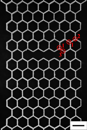
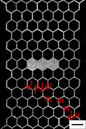
Figure 10: Measured tensile strength of lattice specimens with LABEL:sub@fig:removed_cellswalls_stress a row of missing cell walls and LABEL:sub@fig:filled_cells_stress a row of solid inclusions, as a function of the defect size $a_{\rm 0}/\leavevmode\hbox{\set@color$\ell$}$. Sequence of strut failure in one specimen containing LABEL:sub@fig:hexlattice_cut_32_failure missing cell walls ($a_{0}/\leavevmode\hbox{\set@color$\ell$}=2.6$) or LABEL:sub@fig:hexlattice_cut_21_failure solid inclusion ($a_{0}/\leavevmode\hbox{\set@color$\ell$}=2.6$). The scale bar is of length $10\text{\,}\mathrm{m}\mathrm{m}$.

Centre-cracked lattice specimens were manufactured with a row of missing cell walls at the centre of a regular lattice, see Fig. 2. The initial crack is of semi-length $a_{0}=\sqrt{3}n_{\mathrm{b}}\leavevmode\hbox{\set@color$\ell$}/2$ where $n_{\rm b}$ is the number of broken cell walls. The influence of crack length on the tensile strength of the lattice was explored by varying $n_{\rm b}$ between 0 and 3; three realisations of the lattice were generated for each value of $n_{\mathrm{b}}$. The measured values of the notch tensile strength $\sigma^{\infty}_{\mathrm{f}}$ are plotted in Fig. 10 as a function of the crack length $a_{0}/\leavevmode\hbox{\set@color$\ell$}$, for the choice $\mkern 1.25mu\overline{\mkern-1.25mu\rho\mkern-1.25mu}\mkern 1.25mu=0.11$. A significant drop in $\sigma^{\infty}_{\mathrm{f}}$ is observed when 1 or more struts are broken.

The sensitivity of tensile strength of the lattice to missing cell walls can be rationalised in terms of its transition flaw size $a_{\rm T}$: this is the semi-length of the crack beyond which fracture of the lattice is given by a fracture mechanics assessment. The value of $a_{\rm T}$ for an elastic-brittle lattice depends upon the fracture toughness of the lattice $K_{\rm IC}$ and the tensile strength of an intact, crack-free lattice $\sigma^{\infty}_{\mathrm{f}}(a_{0}=0)$ as [18]

$$a_{\rm T}=\frac{1}{\pi}\left[\frac{K_{\rm IC}}{\sigma^{\infty}_{\rm f}(a_{0}=0)}\right]^{2}$$ (4)

where $K_{\rm IC}$ is expressed in terms of the tensile strength of the cell wall solid $\sigma_{\rm fs}$, relative density of the lattice $\mkern 1.25mu\overline{\mkern-1.25mu\rho\mkern-1.25mu}\mkern 1.25mu$ and strut length $\ell$ according to [20]

$$K_{\rm IC}=0.9\mkern 1.25mu\overline{\mkern-1.25mu\rho\mkern-1.25mu}\mkern 1.25mu^{2}\sigma_{\rm fs}\sqrt{\leavevmode\hbox{\set@color$\ell$}}$$ (5)

Upon substituting Eq. (5) into Eq. (4) and taking $\sigma^{\infty}_{\rm f}(a_{0}=0)$ to be the measured mean strength of crack-free lattice specimens (of $\mkern 1.25mu\overline{\mkern-1.25mu\rho\mkern-1.25mu}\mkern 1.25mu=0.11$), $\sigma^{\infty}_{\rm f}(a_{0}=0)=$0.2\text{\,}\mathrm{M}\mathrm{P}\mathrm{a}$$ (see Fig. 7), we find that $a_{\rm T}=1.4\leavevmode\hbox{\set@color$\ell$}$ for a hexagonal lattice made from solid PMMA of tensile strength $\sigma_{\rm fs}=$36\text{\,}\mathrm{M}\mathrm{P}\mathrm{a}$$. Predictions for the tensile strength, $\sigma^{\infty}_{\rm f}(a_{0})=K_{\rm IC}/\left(Y\sqrt{\pi a_{0}}\right)$, are included in Fig. 10 and they are in good agreement with the measured values. Note that these predictions include the geometric $K-$calibration factor $Y(a_{0}/W,L/W)$ from  Liu [27] to account for the effect of the finite geometry of the specimen. We find from Fig. 10 that the transition from strength-controlled fracture to $K-$controlled fracture occurs at $a_{0}\approx a_{\rm T}=1.4\leavevmode\hbox{\set@color$\ell$}$. For all values of $a_{0}$ explored in this study, a critical strut fails adjacent to the pre-crack followed by a series of strut failures in its immediate vicinity, see Fig. 10 for the case of $a_{0}/\leavevmode\hbox{\set@color$\ell$}=2.6$, in support of this observation.

7.3 Solid inclusions

Hexagonal lattices containing a solid inclusion were generated by the laser-cutting of PMMA sheets, with a number of intact filled cells at the centre of the specimen, recall Fig. 10. The semi-length of the inclusion is $a_{0}=\sqrt{3}n_{\rm c}\leavevmode\hbox{\set@color$\ell$}/2$ where $n_{\rm c}$ is the number of filled cells. Three realisations of the lattice were generated for each value of $n_{\rm c}$ between 0 and 3. The measured values of macroscopic tensile strength $\sigma^{\infty}_{\mathrm{f}}$ are plotted in Fig. 10 as a function of the inclusion size $a_{0}/\leavevmode\hbox{\set@color$\ell$}$: $\sigma^{\infty}_{\mathrm{f}}$ is almost insensitive to the presence of solid inclusions. The location of the failure is remote from the inclusion and it is from the edge of the specimen consistent with the predictions of Chen et al. [28], see Fig. 10 for the case of $a_{0}/\leavevmode\hbox{\set@color$\ell$}=2.6$.

8 Concluding remarks

The present study explores the relative sensitivity of tensile strength of a lattice to as-manufactured defects and as-designed defects. It is found that both classes of defects are significant for an elastic-brittle lattice that has been manufactured by a rapid prototyping route. FE analysis provides insight into the relative potency of defects in controlling both the mean tensile strength and the dispersion in tensile strength of PMMA lattices.

Hexagonal lattices were generated by laser-cutting PMMA sheets, and were tested under uniaxial tension at room temperature; at this temperature, PMMA behaves in an elastic-brittle manner. It is found from both experiments and FE predictions that the uniaxial tensile response of the laser-cut PMMA lattices is linear elastic until a critical strut fails at the edge of the finite specimen (but within the gauge dimensions), recall Fig. 6. In turn, a series of struts adjacent to this failed strut fail in sequence within a relatively small ($<0.5\%$) increment of macroscopic strain, thereby forming a single dominant crack at the edge of the specimen. Such behaviour is consistent with the small transition flaw size ($a_{\rm T}\approx\leavevmode\hbox{\set@color$\ell$}$) for the elastic-brittle hexagonal lattice, as previously discussed by Tankasala et al. [18]. In all lattice specimens tested in this study, failure occurs first in an inclined strut close to the joint, and all failed struts exist within the gauge dimensions of the specimen. The measured values of macroscopic Young’s modulus $E$ and macroscopic tensile strength $\sigma^{\infty}_{\rm f}$ scale with the lattice relative density $\mkern 1.25mu\overline{\mkern-1.25mu\rho\mkern-1.25mu}\mkern 1.25mu$ in accordance with the analytical predictions of Gibson and Ashby [13] based on a point-wise stress-based failure criterion for lattice tensile strength.

Three-dimensional computed tomography analysis of the laser-cut specimens revealed imperfections in the lattice geometry in the form of a dispersion in strut thickness and in Plateau border radius. The influence of these as-manufactured defects was explored by combined experimental and numerical studies. In general, the presence of these defects leads to a reduction in the macroscopic tensile strength of the lattices; a dispersion in strut thickness leads to the largest knockdown in strength. Catastrophic fracture of the specimen occurs by the formation of a single crack emanating from the edge of the specimen and a series of struts fail at an almost-constant value of load. The dispersion in strut thickness is associated with a dispersion in strut tensile strength due to the thermal history imposed on each strut by the laser-based manufacturing process. Additional FE simulations were performed to explore the sensitivity of the macroscopic tensile strength to the dispersion in strut tensile strength. A significant knockdown in macroscopic strength is predicted by the introduction of a minor dispersion in the strut tensile strength.

Imperfections were also introduced in the laser-cut lattices by design. Three kinds of imperfections were explored experimentally: randomly misplaced joints, a row of missing cell walls to create a notch, and a row of cells filled by solid inclusions. The following conclusions can be drawn for each type of defect:

• Imperfections in the form of randomly perturbed joints. The macroscopic modulus of the lattice increases by $40\%$ as $R/\leavevmode\hbox{\set@color$\ell$}$ increases from 0 to 0.5. This finding is in agreement with the numerical prediction of Chen et al. [29] who have reported a similar increase in modulus of an elastic-brittle Voronoi honeycomb compared to that of the regular hexagonal honeycomb. In contrast, the macroscopic tensile strength of the lattice is almost insensitive to the perturbation of nodal position and this is ascribed to the fact that the primary mode of deformation within a failed strut is bending for all values of $R/\leavevmode\hbox{\set@color$\ell$}$ between 0 and 0.5.

• Imperfections in the form of missing cell walls. The notch tensile strength of the centre-cracked lattice ranges from the notch-insensitive limit $\sigma^{\infty}_{\rm f}(a_{0})=\sigma^{\infty}_{\rm f}(0)$ to the value based on fracture toughness, $\sigma^{\infty}_{\rm f}(a_{0})=K_{\rm IC}/(Y\sqrt{\pi a_{0}})$ for increasing semi-crack length $a_{0}$ from $0$ to $3\leavevmode\hbox{\set@color$\ell$}$. The transition flaw size is $a_{\rm T}\approx\leavevmode\hbox{\set@color$\ell$}$, consistent with the numerical predictions of Tankasala et al. [18] for an elastic-brittle hexagonal lattice. In each case, failure of the lattice occurs in a crack-like manner by the successive failure of a series of inclined struts ahead of the initial crack tip.

• Imperfections in the form of solid inclusions. The lattice tensile strength is insensitive to the presence of filled cells; no distinct knockdown in strength is observed for inclusions of size $0$ and $3\leavevmode\hbox{\set@color$\ell$}$. Further, the location of first strut failure is remote from the inclusions and at the edge of the specimen.

In summary, the macroscopic tensile strength of the hexagonal PMMA lattice is most sensitive to imperfections in the form of broken cell walls owing to its low transition flaw size. In contrast, only a mild sensitivity of the tensile strength is observed for the cases of misplaced joints and cells filled with solid inclusions.

Tables

case	$t_{\mathrm{sd}}/\mkern 1.25mu\overline{\mkern-1.25mut\mkern-1.25mu}\mkern 1.25mu$	$r_{\mathrm{sd}}/\mkern 1.25mu\overline{\mkern-1.25mur\mkern-1.25mu}\mkern 1.25mu$	$\mkern 1.25mu\overline{\mkern-1.25mu\sigma\mkern-1.25mu}\mkern 1.25mu^{\infty}_{\mathrm{f}}/\mkern 1.25mu\overline{\mkern-1.25mu\sigma\mkern-1.25mu}\mkern 1.25mu^{\infty}_{\mathrm{Exp}}$	${\sigma}^{\infty}_{\mathrm{f,sd}}/\mkern 1.25mu\overline{\mkern-1.25mu\sigma\mkern-1.25mu}\mkern 1.25mu^{\infty}_{\mathrm{Exp}}$
A	0	0	1.42	0
B	0	0.25	1.29	0.02
C	0.19	0	1.18	0.05
D	0.19	0.25	1.11	0.06
E	0.19	0.25	1.09	0.09
E (Exp.)	0.19	0.25	1	0.17

Table 1: Effect of as-manufactured defects on the tensile strength of lattice specimens. In all cases, $\mkern 1.25mu\overline{\mkern-1.25mut\mkern-1.25mu}\mkern 1.25mu=$0.47\text{\,}\mathrm{m}\mathrm{m}$$ and $\mkern 1.25mu\overline{\mkern-1.25mur\mkern-1.25mu}\mkern 1.25mu=$0.4\text{\,}\mathrm{m}\mathrm{m}$$.

Figures

[figure]subcapbesideposition=top

[]
[] []
[]

[] []
[]

Figure 3: Nominal stress versus nominal strain response of macroscale dogbone-shaped specimens and single strut specimens.

[]
[]

[] []
[]

[] []

Figure 7: Measured values of LABEL:sub@fig:relativeDensity_YoungsModulus_perfectHex macroscopic Young’s modulus $E$, and LABEL:sub@fig:relativeDensity_stressFailure_perfectHex macroscopic tensile strength $\sigma^{\infty}_{\mathrm{f}}$ of regular hexagonal lattice specimens as a function of $\mkern 1.25mu\overline{\mkern-1.25mu\rho\mkern-1.25mu}\mkern 1.25mu$. Unfilled symbols are additional measurements from results from regular lattice specimens of $7\,\times\,13$ cells and dashed lines are predictions as given by Eq. (3).

[] []

Figure 8: Role of dispersion in strut tensile strength within a regular lattice. LABEL:sub@fig:fe_pdf_strutdispersion Assumed normal probability distribution functions for strut tensile strength $\sigma_{\rm fs}$, and LABEL:sub@fig:fe_sf_strutdispersion the normalised macroscopic tensile strength as a function of the dispersion in strut strength $\sigma_{\mathrm{fs,sd}}/\mkern 1.25mu\overline{\mkern-1.25mu\sigma\mkern-1.25mu}\mkern 1.25mu_{\mathrm{fs}}$.

[] []

[] []
[] []

References

- Phani and Hussein [2017] A. S. Phani, M. I. Hussein, Introduction to Lattice Materials, John Wiley & Sons, Ltd, 2017, pp. 1–17.
- Tumbleston et al. [2015] J. R. Tumbleston, D. Shirvanyants, N. Ermoshkin, R. Janusziewicz, A. R. Johnson, D. Kelly, K. Chen, R. Pinschmidt, J. P. Rolland, A. Ermoshkin, et al., Continuous liquid interface production of 3D objects, Science 347 (2015) 1349–1352.
- Vyatskikh et al. [2018] A. Vyatskikh, S. Delalande, A. Kudo, X. Zhang, C. M. Portela, J. R. Greer, Additive manufacturing of 3D nano-architected metals, Nature communications 9 (2018) 593.
- Deshpande et al. [2001] V. S. Deshpande, M. F. Ashby, N. A. Fleck, Foam topology: bending versus stretching dominated architectures, Acta Materialia 49 (2001) 1035–1040.
- Li et al. [2007] K. Li, X.-L. Gao, J. Wang, Dynamic crushing behavior of honeycomb structures with irregular cell shapes and non-uniform cell wall thickness, International Journal of Solids and Structures 44 (2007) 5003–5026.
- Tancogne-Dejean et al. [2016] T. Tancogne-Dejean, A. B. Spierings, D. Mohr, Additively-manufactured metallic micro-lattice materials for high specific energy absorption under static and dynamic loading, Acta Materialia 116 (2016) 14–28.
- Queheillalt and Wadley [2005] D. T. Queheillalt, H. N. Wadley, Pyramidal lattice truss structures with hollow trusses, Materials Science and Engineering: A 397 (2005) 132–137.
- Andrews et al. [1999] E. Andrews, W. Sanders, L. Gibson, Compressive and tensile behaviour of aluminum foams, Materials Science and Engineering: A 270 (1999) 113–124.
- Montemayor et al. [2016] L. Montemayor, W. Wong, Y.-W. Zhang, J. Greer, Insensitivity to flaws leads to damage tolerance in brittle architected meta-materials, Scientific reports 6 (2016).
- Olurin et al. [2000] O. B. Olurin, N. A. Fleck, M. F. Ashby, Deformation and fracture of aluminium foams, Materials Science and Engineering: A 291 (2000) 136–146.
- Ma et al. [2016] Q. Ma, H. Cheng, K.-I. Jang, H. Luan, K.-C. Hwang, J. A. Rogers, Y. Huang, Y. Zhang, A nonlinear mechanics model of bio-inspired hierarchical lattice materials consisting of horseshoe microstructures, Journal of the Mechanics and Physics of Solids 90 (2016) 179–202.
- Gebhardt and Hötter [2016] A. Gebhardt, J.-S. Hötter, Additive manufacturing: 3D printing for prototyping and manufacturing, Carl Hanser Verlag GmbH Co KG, 2016.
- Gibson and Ashby [1999] L. J. Gibson, M. F. Ashby, Cellular solids: structure and properties, Cambridge university press, 1999.
- Ronan et al. [2016] W. Ronan, V. S. Deshpande, N. A. Fleck, The tensile ductility of cellular solids: The role of imperfections, International Journal of Solids and Structures 102-103 (2016) 200–213.
- Symons and Fleck [2008] D. D. Symons, N. A. Fleck, The Imperfection Sensitivity of Isotropic Two-Dimensional Elastic Lattices, Journal of Applied Mechanics 75 (2008) 051011.
- Schmidt and Fleck [2001] I. Schmidt, N. A. Fleck, Ductile fracture of two-dimensional cellular structures, International Journal of Fracture 111 (2001) 327–342.
- Tankasala et al. [2015] H. C. Tankasala, V. S. Deshpande, N. A. Fleck, 2013 Koiter Medal Paper: Crack-Tip Fields and Toughness of Two-Dimensional Elastoplastic Lattices, Journal of Applied Mechanics 82 (2015) 091004.
- Tankasala et al. [2017] H. C. Tankasala, V. S. Deshpande, N. A. Fleck, Tensile response of elastoplastic lattices at finite strain, Journal of the Mechanics and Physics of Solids 109 (2017) 307–330.
- Fleck and Qiu [2007] N. A. Fleck, X. Qiu, The damage tolerance of elastic–brittle, two-dimensional isotropic lattices, Journal of the Mechanics and Physics of Solids 55 (2007) 562–588.
- Romijn and Fleck [2007] N. E. Romijn, N. A. Fleck, The fracture toughness of planar lattices: Imperfection sensitivity, Journal of the Mechanics and Physics of Solids 55 (2007) 2538–2564.
- Grenestedt [2005] J. Grenestedt, On interactions between imperfections in cellular solids, Journal of materials science 40 (2005) 5853–5857.
- Liu et al. [2017] L. Liu, P. Kamm, F. García-Moreno, J. Banhart, D. Pasini, Elastic and failure response of imperfect three-dimensional metallic lattices: the role of geometric defects induced by Selective Laser Melting, Journal of the Mechanics and Physics of Solids 107 (2017) 160–184.
- Onck et al. [2004] P. Onck, R. van Merkerk, J. De Hosson, I. Schmidt, Fracture of Metal Foams: In-situ Testing and Numerical Modeling, Advanced Engineering Materials 6 (2004) 429–431.
- Van Loock and Fleck [2018] F. Van Loock, N. A. Fleck, Deformation and failure maps for PMMA in uniaxial tension, Polymer 148 (2018) 259–268.
- Choi and Salem [1993] S. Choi, J. Salem, Fracture toughness of PMMA as measured with indentation cracks, Journal of Materials Research 8 (1993) 3210–3217.
- Oliver [1989] J. Oliver, A consistent characteristic length for smeared cracking models., International Journal for Numerical Methods in Engineering 28 (1989) 461–474.
- Liu [1996] A. Liu, Summary of stress-intensity factors, ASM International (1996) 980–1000.
- Chen et al. [2001] C. Chen, T. J. Lu, N. A. Fleck, Effect of inclusions and holes on the stiffness and strength of honeycombs, International Journal of Mechanical Sciences 43 (2001) 487–504.
- Chen et al. [1999] C. Chen, T. J. Lu, N. A. Fleck, Effect of imperfections on the yielding of two-dimensional foams, Journal of the Mechanics and Physics of Solids 47 (1999) 2235–2272.