Amplitude Estimation without Phase Estimation

Abstract

This paper focuses on the quantum amplitude estimation algorithm, which is a core subroutine in quantum computation for various applications. The conventional approach for amplitude estimation is to use the phase estimation algorithm, which consists of many controlled amplification operations followed by a quantum Fourier transform. However, the whole procedure is hard to implement with current and near-term quantum computers. In this paper, we propose a quantum amplitude estimation algorithm without the use of expensive controlled operations; the key idea is to utilize the maximum likelihood estimation based on the combined measurement data produced from quantum circuits with different numbers of amplitude amplification operations. Numerical simulations we conducted demonstrate that our algorithm asymptotically achieves nearly the optimal quantum speedup with a reasonable circuit length.

1 Introduction

Quantum computers are expected to allow us to perform high-speed computations over classical computations for problems in a wide range of scientific and technological fields. Environments in which quantum algorithms can be executed by real quantum devices are currently being provided IBMQ2019 ; PhysRevX.8.021012 ; PhysRevLett.119.180511 . Real quantum devices with several tens of qubits will soon be realized in near future, although those are the so-called noisy intermediate-scale quantum (NISQ) devices that impose several practical limitations on their use Preskill2018 , both in the number of gate operations and the number of available qubits. Hence, several custom subroutines taking into account these constraints have been proposed, typically the variational quantum eigensolver McClean2016 ; Yung2014 .

In this paper, we focus on the amplitude estimation algorithm, which is a core subroutine in quantum computation for various applications, e.g., in chemistry Knill2007 ; Guzik2008 , finance Bromley2018 ; Woerner2019 , and machine learning Wiebe2015 ; Wiebe2016a ; Wiebe2016b ; Kerenidis2018 . In particular, quantum speedup of Monte Carlo sampling via amplitude estimation Montanaro2015 lies in the heart of these applications. Therefore, in light of its importance, we followed the aforementioned direction and developed a new amplitude estimation algorithm that can be executed in NISQ devices.

Note that Ref. Brassard2002 demonstrated that the amplitude estimation problem can be formulated as a phase estimation problem kitaev1996quantum , where the amplitude to be estimated is inferred from the eigenvalue of the corresponding amplification operator. Owing to the ubiquitous nature of the eigenvalue estimation problem, some versions of the phase estimation algorithm suitable for NISQ devices Svore2013 ; Granade2016 ; OBrien2018 ; denBerg2019 ; CRWie2019 have been proposed (with the last one appeared slightly after ours), and they all rely on classical post-processing statistics such as the Bayes method. However, these modified phase estimation algorithms as well as the original scheme kitaev1996quantum still involve many controlled operations (e.g., the controlled amplification operation in the case of Ref. Brassard2002 ) that can be difficult to implement on NISQ devices. Therefore, a new algorithm specialized to the amplitude estimation problem is required, one that does not use expensive controlled operations.

The goal of amplitude estimation is, in its simplest form, to estimate the unknown parameter $\theta$ contained in the state $\left|\Psi\right>=\sin\theta\left|{\rm good}\right>+\cos\theta\left|{\rm bad}\right>$, where $\left|{\rm good}\right>$ and $\left|{\rm bad}\right>$ are given orthogonal state vectors. Our scheme is composed of the amplitude amplification process and the maximum likelihood (ML) estimation; the controlled operations and the subsequent quantum Fourier transform (QFT) are not involved. The amplification process transforms the coefficient of $\left|{\rm good}\right>$ to $\sin((2m+1)\theta)$ with $m$ being the number of operations; if $\theta$ is known, then, by suitably choosing $m$, we can enhance the probability of hitting “good” quadratically greater than the classical case, where no amplitude amplification is utilized Grover1996 . However, the function $\sin((2m+1)\theta)$ does not always take a relatively large value for a certain $m$ because $\theta$ is unknown in this problem, meaning that an effective quantum speedup is not always available; also, the ML estimate is not uniquely determined due to the periodicity of this function. Our strategy is the first to make measurements on the transformed quantum state and to construct likelihood functions for several $m$, say $\{m_{0},\ldots,m_{M}\}$, and then combine them to construct a single likelihood function that uniquely produces the ML estimate; see Fig. 1. The broad concept behind this scheme is to combine the data produced from different quantum circuits, and the scheme might be performed even on NISQ devices to compute a target value faster than classical algorithms via some post-processing. Actually a numerical simulation demonstrates that, by appropriately designing $\{m_{k}\}$, compared with the classical sampling we can achieve nearly a square-root reduction in the total number of queries to reach the specified estimation precision; notably, only relatively short-depth circuits are required to achieve this quantum speedup. We also show that, in an application of the amplitude estimation to Monte Carlo integration, our algorithm requires many fewer controlled NOT (CNOT) gates than the conventional phase-estimation-based approach, so it is suitable for obtaining quantum advantages with NISQ devices. Note that Ref. Abrams1999 also took the approach without using the phase estimation method, but it needed to change the query in each iteration, which is highly demanding in practice. Also the paper Ref. Zintchenko2016 gave an amplitude estimation scheme that employs a Bayes rule together with applying random Unitary operations (subjected to the Haar measure) to ideally realize the quadratic speedup, without a controlled Unitary operation; this scheme is applicable to low-dimensional quantum circuits, due to the hardness to implement the random Unitaries.

2 Preliminary

We herein briefly describe the quantum amplitude amplification, which is the basis of our approach for the amplitude estimation problem.

Our proposed algorithm mainly consists of two parts: quantum amplitude amplification and amplitude estimation based on likelihood analysis. The amplitude amplification Brassard1997 ; Grover1998 is the generalization of the Grover’s quantum searching algorithm Grover1996 . Similar to quantum searching, the amplitude amplification is known to achieve quadratic speedup over the corresponding classical algorithm.

We assume a unitary operator $\mathcal{A}$ that acts on $(n+1)$ qubits, such that $\ket{\Psi}=\mathcal{A}\ket{0}_{n+1}=\sqrt{a}\ket{\tilde{\Psi}_{1}}\ket{1}+\sqrt{1-a}\ket{\tilde{\Psi}_{0}}\ket{0}$, where $a\in\left[0,1\right]$ is the unknown parameter to be estimated, while $\ket{\tilde{\Psi}_{1}}$ and $\ket{\tilde{\Psi}_{0}}$ are the $n$-qubit normalized good and bad states. The query complexity of estimating $a$ is counted by the number of the operations of $\mathcal{A}$, which is often denoted as the number of queries for simplicity. By performing measurements on $\ket{\Psi}$ repeatedly, we can infer $a$ from the ratio of obtaining the good and bad states, but the number of queries is exactly the same as the classical one in this case.

The advantage offered by the quantum amplitude amplification is that, instead of measuring right after the single operation of $\mathcal{A}$, we can amplify the probability of obtaining the good state by applying the following operator.

$$\mathbf{Q}=-\mathcal{A}\mathbf{S}_{0}\mathcal{A}^{-1}\mathbf{S}_{\chi},$$ (1)

where the operator $\mathbf{S}_{\chi}$ puts a negative sign to the good state, i.e., $\mathbf{S}_{\chi}\ket{\tilde{\Psi}_{1}}\ket{1}=-\ket{\tilde{\Psi}_{1}}\ket{1}$, and does nothing to the bad state. Similarly, $\mathbf{S}_{0}$ puts a negative sign to the all-zero state $\ket{0}_{n+1}$ and does nothing to the other states. $\mathcal{A}^{-1}$ is the inverse of $\mathcal{A}$, the operation of which requires the same query complexity as $\mathcal{A}$.

By defining a parameter $\theta_{a}\in\left[0,\pi/2\right]$ such that $\sin^{2}{\theta_{a}}=a$, we have

$$\mathcal{A}\ket{0}_{n+1}=\sin{\theta_{a}}\ket{\tilde{\Psi}_{1}}\ket{1}+\cos{\theta_{a}}\ket{\tilde{\Psi}_{0}}\ket{0}.$$ (2)

Brassard et al. Brassard2002 showed that repeatedly applying $\mathbf{Q}$ for $m$ times on $\ket{\Psi}$ results in

$$\mathbf{Q}^{m}\ket{\Psi}=\sin((2m+1)\theta_{a})\ket{\tilde{\Psi}_{1}}\ket{1}+\cos((2m+1)\theta_{a})\ket{\tilde{\Psi}_{0}}\ket{0}.$$ (3)

This equation represents that, after applying $\mathbf{Q}$ $m$ times (with $2m$ queries), we can obtain the good state with a probability of at least $4m^{2}$ times larger than that obtained from $\mathcal{A}\ket{0}_{n+1}$ for sufficiently small $a$. This is in contrast with having $2m$ number of measurements from $\mathcal{A}\ket{0}_{n+1}$, which only gives the good state with probability $2m$ times larger. This intuitively gives the quadratic speedup obtained from the amplitude amplification: if we can infer the ratio of the good state after the amplitude amplification, we can estimate the value of $a$ from the number of queries required to obtain such a ratio.

The conventional amplitude estimationBrassard2002 utilizes the quantum phase estimation which requires a quantum circuit that implements the multiple controlled $\mathbf{Q}$ operations, namely, $\mbox{Controlled-}\mathbf{Q}:~{}\ket{m}\ket{\Psi}\rightarrow\ket{m}\mathbf{Q}^{m}\ket{\Psi}$. Performing the controlled operations simultaneously on many $m$’s consecutively and gathering the amplitude by the inverse QFT enables an accurate estimation of $a$ Brassard2002 . However, this approach suffers from the need for many controlled gates (thus, CNOT gates) and additional ancilla qubits (the number of which is dictated by the required accuracy). Such an approach can be problematic for NISQ devices.

3 Amplitude estimation without phase estimation

3.1 Algorithm

This section shows the quantum algorithm to estimate $\theta_{a}$ in Eq. (3) without using the conventional phase-estimation-based method Brassard2002 . The first stage of the algorithm is to make good or bad measurements on the quantum state ${\mathbf{Q}}^{m_{k}}\ket{\Psi}$ for a chosen set of $\{m_{k}\}$. Let $N_{k}$ be the number of measurements (shots) and $h_{k}$ be the number of measuring good states for the state ${\mathbf{Q}}^{m_{k}}\ket{\Psi}$; then, because the probability measuring the good state is $\sin^{2}((2m_{k}+1)\theta_{a})$, the likelihood function representing this probabilistic event is given by

$$L_{k}(h_{k};\theta_{a})=\left[\sin^{2}((2m_{k}+1)\theta_{a})\right]^{h_{k}}\left[\cos^{2}((2m_{k}+1)\theta_{a})\right]^{N_{k}-h_{k}}.$$ (4)

The second stage of the algorithm is to combine the likelihood functions $L_{k}(h_{k};\theta_{a})$ for several $\{m_{0},\ldots,m_{M}\}$ to construct a single likelihood function $L(\vec{h};\theta_{a})$:

$$L(\vec{h};\theta_{a})=\prod_{k=0}^{M}L_{k}(h_{k};\theta_{a}),$$ (5)

where $\vec{h}=(h_{0},h_{1},\cdots,h_{M})$. The ML estimate is defined as the value that maximizes $L(\vec{h};\theta_{a})$:

$$\hat{\theta}_{a}=\mathop{\rm arg~{}max}\limits_{\theta_{a}}~{}L(\vec{h};\theta_{a})=\mathop{\rm arg~{}max}\limits_{\theta_{a}}~{}\ln L(\vec{h};\theta_{a})$$ (6)

The whole procedure is summarized in Fig. 1. Now $a$ and $\theta_{a}$ are uniquely related through $a=\sin^{2}\theta_{a}$ in the range $0\leq\theta_{a}\leq\pi/2$, and $\hat{a}:=\sin^{2}\hat{\theta}_{a}$ is the ML estimate for $a$; thus, in what follows, $L(\vec{h};a)$ is denoted as $L(\vec{h};\theta_{a})$. Note that the random variables $h_{0},h_{1},\ldots,h_{M}$ are independent but not identically distributed because the probability distribution for obtaining $h_{k}$, i.e., $p_{k}(h_{k};\theta_{a})\propto L_{k}(h_{k};\theta_{a})$, is different for each $k$; however, the set of multidimensional random variables $\vec{h}=(h_{0},h_{1},\cdots,h_{M})$ is independently generated from the identical joint probability distribution $p(\vec{h};\theta_{a})\propto L(\vec{h};\theta_{a})$.

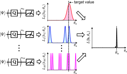
Figure 1: Schematic picture of our amplitude estimation algorithm using the ML estimation. After preparing the states $\mathbf{Q}^{m_{k}}\ket{\Psi}$, the numbers of measuring good states, i.e. $h_{k}$ are obtained (left). Based on the obtained $h_{k}$, the likelihood functions $L_{k}(h_{k};\theta_{a})$ are constructed (center). Finally, a single likelihood function $L(\mathbf{h};\theta_{a})$ is introduced by combining the likelihood functions $L_{k}(h_{k};\theta_{a})$ (right). The ML estimate is the value that maximizes the likelihood function $L(\mathbf{h};\theta_{a})$.

This algorithm has two caveats: (i) if only a single amplitude amplification circuit is used like in the Grover search algorithm, i.e., the case $M=0$ and $m_{0}\neq 0$, the ML estimate $\hat{\theta}_{a}$ cannot be uniquely determined due to the periodicity of $L_{0}(h_{0};\theta_{a})$, and (ii) if no amplification operator is applied, i.e., $m_{k}=0~{}\forall k$, then the ML estimate is unique, but it does not have any quantum advantages, as shown later. Hence, the heart of our algorithm can be regarded as the quantum circuit fusion technique that combines some quantum circuits to determine the target value uniquely, while some quantum advantage is guaranteed.

3.2 Statistics: Cramér–Rao bound and Fisher information

The remaining to be determined in our algorithm was to design the sequences $\{m_{k},N_{k}\}$ so that the resulting ML estimate $\hat{\theta}_{a}$ might have a distinct quantum advantage over the classical one. Here, we introduce a basic statistical method to carry out this task and, based on that method, give some specific choice of $\{m_{k},N_{k}\}$.

First, in general, the Fisher information $\mathcal{I}(a)$ is defined as

$$\mathcal{I}(a)={\mathbb{E}}\left[\left(\frac{\partial}{\partial a}\ln L(x;a)\right)^{2}\right],$$ (7)

where the expectation is taken over a random variable $x$ subjected to a given probability distribution $p(x;a)$ with an unknown parameter $a$. The importance of the Fisher information can be clearly seen from the fact that any estimate $\hat{a}$ satisfies the following Cramér–Rao inequality.

$${\rm{var}}(\hat{a})=\mathbb{E}[(\hat{a}-\mathbb{E}[\hat{a}])^{2}]\geq\frac{[1+b^{\prime}(a)]^{2}}{{\mathcal{I}}(a)},$$ (8)

where $b(a)$ represents the bias defined by $b(a)=\mathbb{E}[\hat{a}-a]$ and $b^{\prime}(a)$ indicates the derivative of $b(a)$ with respect to $a$. It is easy to see that the mean squared estimation error satisfies

$$\mathbb{E}[(\hat{a}-a)^{2}]\geq\frac{[1+b^{\prime}(a)]^{2}}{{\mathcal{I}}(a)}+b(a)^{2}.$$ (9)

A specifically important property of the ML estimate, which maximizes the likelihood function $\prod_{k}p({x}_{k};a)$ with the measurement data ${x}_{k}$, is that it becomes unbiased, i.e., $b(a)=0$, and further achieves the equality in Eq. (9) in the large number limit of measurement data rao1973linear ; that is, the ML estimate is asymptotically optimal.

In our case, by substituting Eqs. (4) and (5) into Eq. (7) together with a straight forward calculation $\mathbb{E}[h_{k}]=N_{k}\sin^{2}((2m_{k}+1)\theta_{a})$, we find that

$${\mathcal{I}(a)}=\frac{1}{a(1-a)}\sum_{k=0}^{M}{N_{k}}(2m_{k}+1)^{2}.$$ (10)

Also, for any sequences $\{m_{k},N_{k}\}$, the total number of queries is given as

$$N_{\rm{q}}=\sum_{k=0}^{M}N_{k}(2m_{k}+1).$$ (11)

As stated before, the coefficient $2$ multiplying $m_{k}$ in Eq. (11) originates from the fact that the operator $\mathbf{Q}$ uses $\mathcal{A}$ and $\mathcal{A}^{-1}$, and the constant $+1$ is due to the initial state preparation of $\ket{\Psi}=\mathcal{A}\ket{0}_{n+1}$. If $\mathbf{Q}$ is not applied to $\ket{\Psi}$ and if only the final measurements are performed for $\ket{\Psi}$, i.e., $m_{k}=0$ for all $k$, the total number of queries is identical to that of classical random sampling. Because $N_{k}$ and $(2m_{k}+1)$ are positive integers, the Fisher information in Eq. (10) satisfies the following relation.

$${\mathcal{I}}(a)~{}\leq~{}\frac{1}{a(1-a)}\left(\sum_{k=0}^{M}N_{k}(2m_{k}+1)\right)^{2}~{}=~{}\frac{1}{a(1-a)}N_{\rm{q}}^{2}.$$ (12)

Here, $\hat{a}$ is set to the ML estimate (6), and the estimation error is considered to be $\hat{\epsilon}=\sqrt{\mathbb{E}[(\hat{a}-a)^{2}]}$ in this case. The total number of measurements $\sum_{k=0}^{M}N_{k}$ is assumed to be sufficiently large, in which case the ML estimate asymptotically converges to an unbiased estimate and achieves the lower bound of the Cramér–Rao inequality (8), as aforementioned. Hence, from Eqs. (8) and (12), the error $\hat{\epsilon}$ satisfies

$$\hat{\epsilon}\rightarrow\frac{1}{{\mathcal{I}}(a)^{1/2}}\geq\frac{\sqrt{a(1-a)}}{N_{\rm{q}}}.$$ (13)

(More precisely, $\hat{\epsilon}\,\mathcal{I}(a)^{1/2}\rightarrow 1$.) That is, the lower bound of the estimation error is on the order of $\mathcal{O}(N_{\rm{q}}^{-1})$, which is referred to as the Heisenberg limit. This is in stark contrast to the classical sampling method, the estimation error of which is lower bounded by $\sqrt{a(1-a)}/N_{\rm{q}}^{1/2}$, obtained by setting $m_{k}=0~{}\forall k$ (i.e., a case with no amplitude amplification) in Eqs. (10) and (11); that is, the lower bound is at best on the order of $\mathcal{O}(N_{\rm{q}}^{-1/2})$ in the classical case.

Now, we can consider the problem posed at the beginning of this subsection: designing the sequences $\{m_{k},N_{k}\}$ so that the resulting ML estimate $\hat{\theta}_{a}$ outperforms the classical limit $\mathcal{O}(N_{\rm{q}}^{-1/2})$ and hopefully achieves the Heisenberg limit $\mathcal{O}(N_{\rm{q}}^{-1})$, i.e., the quantum quadratic speedup. Although the problem can be formulated as a maximization problem of Fisher information (10) with respect to $\{m_{k},N_{k}\}$ under some constraints on these variables, here we fix $N_{k}$’s to a constant and provide just two examples of the sequence $\{m_{k}\}$:

• Linearly incremental sequence (LIS): $N_{k}=N_{\rm{shot}}$ for all $k$, and $m_{k}=k$, i.e., it increases as $m_{0}=0,m_{1}=1,m_{2}=2,\cdots,m_{M}=M$.

• Exponentially incremental sequence (EIS): $N_{k}=N_{\rm{shot}}$ for all $k$, and $m_{k}$ increases as $m_{0}=0,m_{1}=2^{0},m_{2}=2^{1},\cdots,m_{M}=2^{(M-1)}$.

In the case of LIS, the Fisher information (7) and the number of queries (11) are calculated as ${\mathcal{I}}(a)=N_{\rm{shot}}(2M+3)(2M+1)(M+1)/(3a(1-a))$ and $N_{\rm{q}}=N_{\rm{shot}}(M+1)^{2}$, respectively. Because $N_{\rm{q}}\sim N_{\rm{shot}}M^{2}$ and ${\mathcal{I}}(a)\sim N_{\rm{shot}}M^{3}/(3a(1-a))$ when $M\gg 1$, the lower bound of the estimation error is evaluated as $\hat{\epsilon}=1/{\mathcal{I}}(a)^{1/2}\sim N_{\rm{q}}^{-3/4}$; hence, a distinct quantum advantage occurs, although it does not reach the Heisenberg limit. Next for the case of EIS, we find $N_{\rm{q}}\sim N_{\rm{shot}}2^{M+1}$ and $\mathcal{I}(a)\sim N_{\rm{shot}}2^{2(M+1)}/3$, which as a result lead to $\hat{\epsilon}\sim N_{\rm{q}}^{-1}$. Therefore, this choice is asymptotically optimal; we again emphasize that the statistical method certainly serves as a guide for us to find an optimal sequence $\{m_{k}\}$, achieving an optimal quantum amplitude estimation algorithm. But note that these quantum advantages are guaranteed only in the asymptotic regime and that the realistic performance with the finite (or rather short) circuit depth should be analyzed. We will carry out a numerical simulation to see this realistic case in the following.

3.3 Numerical simulation

In this section, the ML estimates $\hat{\theta}_{a}$ and errors $\hat{\epsilon}$ are evaluated numerically for several fixed target probabilities $a=\sin^{2}\theta_{a}$. Based on the chosen sequence of $\{N_{k}\}$ and $\{m_{k}\}$ shown in the previous subsection, $h_{k}$’s in Eq. (5) are generated using the Bernoulli sampling with probability $\sin^{2}((2m_{k}+1)\theta_{a})$ for each $k$. The global maximum of the likelihood function can be obtained by using a modified brute-force search algorithm; the global maximum of $\prod_{k=0}^{m}L_{k}(h_{k};\theta_{a})$ is determined by searching around the vicinity of the estimated global maximum for $\prod_{k=0}^{m-1}L_{k}(h_{k};\theta_{a})$. The errors $\hat{\epsilon}$ are evaluated by repeating the aforementioned procedures 1000 times for each $N_{\rm{q}}$.

In Fig. 2, the relationship between the number of queries and errors are plotted for the target probabilities $a=\sin^{2}\theta_{a}=2/3$, $1/3$, $1/6$, $1/12$, $1/24$, and $1/48$ with $N_{\textrm{shot}}=100$. The (red) triangles and (black) circles in Fig. 2 are errors that are obtained using LIS and EIS, respectively. For comparison, numerical simulations with $m_{k}=0$ for all $k$ are also performed, and the results are plotted as (blue) squares in Fig. 2. In addition, the lower bounds of errors (13) when the estimate is not biased are also plotted as (red) dotted and (black) solid lines for LIS and EIS, respectively. The (blue) dashed lines in Fig. 2 are the lower bounds for classical random sampling, i.e., $\sqrt{a(1-a)/N_{\rm{q}}}$.

The slopes of the simulated results with the target probability $a=\sin^{2}\theta_{a}=1/48$ ranging from $N_{\rm{q}}\simeq 10^{3}$ to $N_{\rm{q}}\simeq 10^{5}$ in Fig. 2 are fitted by $\log\hat{\epsilon}=\gamma\cdot\log N_{\rm{q}}+\delta$, and the fitted parameters corresponding to the slope are obtained as $\gamma=-0.76$, $\gamma=-0.95$ and $\gamma=-0.50$ for LIS and EIS, and classical random sampling, respectively. Similar slopes are obtained with other target probabilities. The fitted values of $\gamma$ for LIS and EIS are consistent with the slopes obtained using the Fisher information, although $\gamma$ slightly deviated from the theoretical values. This slight deviation indicates that $\hat{a}$ is a biased estimate; in fact, this deviation decreases as $N_{\textrm{shot}}$ increases, which is consistent with the fact that, in general, the ML estimate becomes unbiased asymptotically as the sampling number increases. Also, the efficiency of the ML estimate can be observed in the numerical simulation; the estimation error approaches the Cramér–Rao lower bound (13). In Appendix A, we show the comparison of the error for the conventional phase-estimation-based approach with that of EIS. As a result, their estimation errors are found to be comparable.

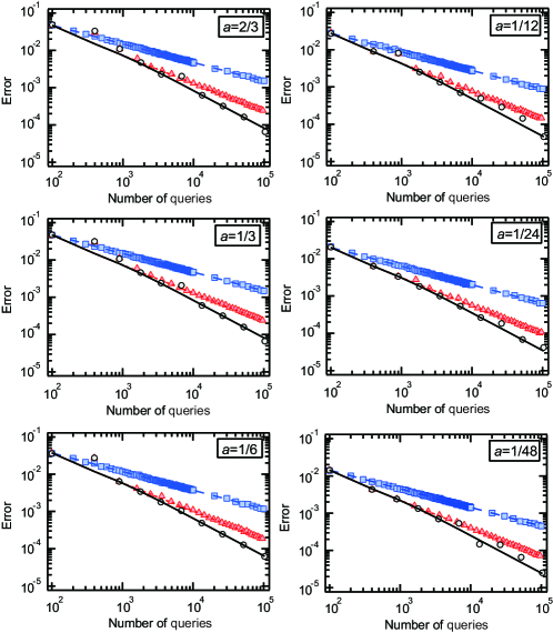
Figure 2: Relationships between the number of queries and the estimation error for several target probabilities $a=\sin^{2}\theta_{a}$. The lower bounds of estimation error based on the Cramér–Rao inequality are depicted as lines, the (blue) dashed line is for $m_{k}=0$ for all $k$ (classical random sampling), the (red) dotted line is for $m_{0}=0,m_{1}=1,\cdots,m_{M}=M$ (LIS), and the (black) solid line is for $m_{0}=0,m_{1}=2^{0},\cdots,m_{M}=2^{M-1}$ (EIS), respectively. The estimation errors obtained by numerical simulations are also plotted as symbols, the (blue) squares are for classical random sampling, the (red) triangles are for LIS, and the (black) circles are for EIS.

Finally, we remark that the computational complexity for naively finding the maximum of the likelihood function is on the order of $\mathcal{O}((1/\epsilon)\ln(1/\epsilon))$ if $m_{k}$ exponentially grows, as in EIS. This is because the computational complexity to obtain the likelihood function $\ln L(\vec{h};\theta_{a})$ is evaluated as $\mathcal{O}(M)$ in this case. The order of the error $\epsilon$ is estimated as $\mathcal{O}(N_{\rm{q}}^{-1})$ based on the Cramér–Rao bound. Because $N_{\rm{q}}\sim 2^{M}N_{\rm{shot}}$, the complexity of evaluating the likelihood function is $\mathcal{O}(\ln(1/\epsilon))$. Assuming that the brute-force search among $1/\epsilon$ segments is performed to find the global maximum of the likelihood function, the complexity of finding the maximum is $\mathcal{{O}}((1/\epsilon)\ln(1/\epsilon))$. In the case of LIS, the order of the computational complexity can also be evaluated as $\mathcal{O}(\epsilon^{-5/3})$ in the same manner as before. It should be noted that the brute-force search algorithm for finding global minima of $\prod_{k=0}^{M}L_{k}(h_{k};\theta_{a})$ is not necessary if $m_{k}$ is zero for all $k$ (classical case), since the target value is simply obtained by $\hat{a}=\sum_{k=0}^{M}h_{k}/\sum_{k=0}^{M}N_{\rm{shot}}$. The error can be obtained as $\mathcal{O}(N_{\rm{q}}^{-1/2})$ based on the Cramér–Rao bound. Due to the fact that $N_{\rm{q}}=N_{\rm{shot}}M$, the computational complexity in the classical case is $\mathcal{O}(\epsilon^{-2})$. The evaluated computational complexities of post-processing for different update rules of $m_{k}$ are summarized together with the query complexities in Table LABEL:complexity.

Table 1: The summary of the complexities for estimating target value with given error $\epsilon$. The query complexity and computational complexity of post-processing for different update rules of $m_{k}$ are listed.

update rule of $m_{k}$	query complexity	computational complexity of
		post-processing
Classical
($m_{k}=0$ $\forall k$)	$\mathcal{O}(\epsilon^{-2})$	$\mathcal{O}(\epsilon^{-2})$
Linearly incremental sequence (LIS)
($m_{0}=0,m_{1}=1,m_{2}=2,\cdots,m_{M}=M$)	$\mathcal{O}(\epsilon^{-4/3})$	$\mathcal{O}(\epsilon^{-5/3})$
Exponentially incremental sequence (EIS)
($m_{0}=0,m_{1}=2^{0},m_{2}=2^{1},\cdots,m_{M}=2^{(M-1)})$	$\mathcal{O}(\epsilon^{-1})$	$\mathcal{O}(\epsilon^{-1}\ln\epsilon^{-1})$

4 Application to the Monte Carlo integration

We conduct a Monte Carlo integration as an example of the application of our algorithm, as follows. In this section, we first review the quantum algorithm to calculate the Monte Carlo integration by amplitude estimation Montanaro2015 and then explain the amplitude amplification operator used in our algorithm. Next, we present the integral of the sine function as a simple example of Monte Carlo integration. Using this example, we discuss the number of CNOT gates and qubits required for our algorithm and the conventional amplitude estimation Brassard2002 .

4.1 The Monte Carlo integration as an amplitude estimation

One purpose of the Monte Carlo integration is to calculate the expected value of real valued function $0\leq f(x)\leq 1$ defined for $n$-bit input $x\in\{0,1\}^{n}$ with probability $p(x)$:

$$\mathbb{E}[f(x)]=\sum_{x=0}^{2^{n}-1}p(x)f(x).$$ (14)

In the quantum algorithm for the Monte Carlo integration, an additional (ancilla) qubit is introduced and assumed to be rotated as

$$\mathcal{R}\ket{x}_{n}\ket{0}=\ket{x}_{n}\left(\sqrt{f(x)}\ket{1}+\sqrt{1-f(x)}\ket{0}\right),$$ (15)

where $\mathcal{R}$ is a unitary operator acting on $n+1$ qubits. In addition, an algorithm $\mathcal{P}$ is introduced, and operating $\mathcal{P}$ to $n$-qubit resister $\ket{0}_{n}$ yields

$$\mathcal{P}\ket{0}_{n}=\sum_{x=0}^{2^{n}-1}\sqrt{p(x)}\ket{x}_{n},$$ (16)

where all qubits in $\ket{0}_{n}$ are in the state $\ket{0}$. Operating $\mathcal{R(P\otimes\mathbf{I}_{\rm{1}})}$ to the state $\ket{0}_{n}\ket{0}$ generates $\ket{\Psi}$:

$$\ket{\Psi} = \mathcal{R(P\otimes\mathbf{I}_{\rm{1}})}\ket{0}_{n}\ket{0}$$ (17)

$$= \sum_{x=0}^{2^{n}-1}\sqrt{p(x)}\ket{x}_{n}\left(\sqrt{f(x)}\ket{1}+\sqrt{1-f(x)}\ket{0}\right),$$ (18)

where $\mathbf{I}_{\rm{1}}$ is the identity operator acting on an ancilla qubit. For convenience, we put $a=\sum_{x=0}^{2^{n}-1}p(x)f(x)$ and introduce two orthonormal bases:

$$\ket{\tilde{\Psi}_{1}} = \frac{1}{\sqrt{a}}\sum_{x=0}^{2^{n}-1}\sqrt{p(x)}\sqrt{f(x)}\ket{x}_{n}\ket{1},$$ (19)

$$\ket{\tilde{\Psi}_{0}} = \frac{1}{\sqrt{1-a}}\sum_{x=0}^{2^{n}-1}\sqrt{p(x)}\sqrt{1-f(x)}\ket{x}_{n}\ket{0}.$$ (20)

By using these bases, the state $\ket{\Psi}$ can be rewritten as

$$\ket{\Psi}=\sqrt{a}\ket{\tilde{\Psi}_{1}}+\sqrt{1-a}\ket{\tilde{\Psi}_{0}}.$$ (21)

Then, the square root of expected value $a=\mathbb{E}[f(x)]$ appears in the amplitude of $\ket{\tilde{\Psi}_{1}}$, and the Monte Carlo integration can be regarded as an amplitude estimation of $\ket{\tilde{\Psi}_{1}}$. The operator $\mathbf{Q}$ defined in Eq. (1) can be achieved using $\mathbf{U}_{\Psi}\mathbf{U}_{\tilde{\Psi}_{0}}$, where $\mathbf{U}_{\tilde{\Psi}_{0}}=\mathbf{I}-2\ket{\tilde{\Psi}_{0}}\bra{\tilde{\Psi}_{0}}$, $\mathbf{U}_{\Psi}=\mathbf{I}-2\ket{\Psi}\bra{\Psi}$, and $\mathbf{I}$ is the identity acting on $n+1$ qubits Brassard2002 . In terms of a practical point of view, we use $\mathbf{U}_{\tilde{\Psi}_{0}}=\mathbf{I}_{n+1}-2\mathbf{I}_{n}\ket{0}\bra{0}$, where $\mathbf{I}=\mathbf{I}_{n+1}=\mathbf{I}_{n}\otimes(\ket{0}\bra{0}+\ket{1}\bra{1})$. By putting $a=\sin^{2}\theta_{a}$ and using Eq. (3), we could apply our algorithm to the Monte Carlo integration. The circuit diagram of the amplitude amplification used in our algorithm is shown in Fig. LABEL:fig:circuit_Grover_schematic. Note that the multi-qubit gate consisting of $\mathcal{P}$ and $\mathcal{R}$ in Fig. LABEL:fig:circuit_Grover_schematic corresponds to the quantum algorithm $\mathcal{A}$ shown in Sec. 2, and the only ancilla qubit for each $k$ is measured when our algorithm is applied to the Monte Carlo. Similarly, the circuit of the conventional amplitude estimation Brassard2002 is shown in Fig. LABEL:fig:circuit_amplitudeEstimation_schematic. In the following, we applied our algorithm to a very simple integral of the sine function and compared the number of CNOT gates and qubits with the results of the conventional amplitude estimation.

4.2 Simple example: integral of the sine function

As a simple example of the Monte Carlo integration, the following integral is considered.

$$I=\frac{1}{b_{\textrm{max}}}\int_{0}^{b_{\textrm{max}}}\sin(x)^{2}dx,$$ (22)

where $b_{\textrm{max}}$ is a constant that determines the upper limit of the integral. By discretizing this integral in $n$-qubit, we obtain

$$S=\sum_{x=0}^{2^{n}-1}p\left(x\right)\sin^{2}\left(\frac{\left(x+\frac{1}{2}\right)b_{\textrm{max}}}{2^{n}}\right),$$ (23)

where $p(x)=\frac{1}{2^{n}}$ is a discrete uniform probability distribution. We now explicitly describe the operators $\mathcal{P}$ and $\mathcal{R}$ for applying our algorithm to calculate the sum (23). The operator $\mathcal{P}$ acting on the $n$-qubit initial state can be defined as

$$\mathcal{P}:\ket{0}_{n}\ket{0}\to\frac{1}{\sqrt{2^{n}}}\sum_{x=0}^{2^{n}-1}\ket{x}_{n}\ket{0}.$$ (24)

The operator $\mathcal{P}$ can be constructed using $n$ Hadamard gates. The operator $\mathcal{R}$ acting on the $(n+1)$-qubit state $\ket{x}_{n}\ket{0}$ can be defined as

$$\mathcal{R}:\ket{x}_{n}\ket{0}\to\ket{x}_{n}\left(\sin\left(\frac{\left(x+\frac{1}{2}\right)b_{\textrm{max}}}{2^{n}}\right)\ket{1}+\cos\left(\frac{\left(x+\frac{1}{2}\right)b_{\textrm{max}}}{2^{n}}\right)\ket{0}\right).$$ (25)

The operator $\mathcal{R}$ can be constructed using controlled Y-rotations as illustrated in Fig. LABEL:fig:circuit_R.